1

Variational Method in Deriving K0

By Farid A. Chouery1, P.E., S.E.

©2006 Farid Chouery all rights reserved

Abstract

In this paper it is shown that K0 , the at rest earth pressure coefficient, can be related

theoretically to failure parameters of soil (c and φ). The approach is to use failure

mechanism that causes the soil to fail while keeping the at rest lateral pressure.

Variational method is used to derive the real K0. An approximate and a closed form

derivation are obtained in sand. The approximate solution gives an equation for K0

identical to the traditional equation by Jáky. The closed form equation shows a slightly

higher K0 value and gives a better comparison with experiments. The resulting failure

surface is successfully compared to rigidly reinforced soil walls. Further analysis was

done to obtain a reasonable approximation of K0 for clay and overconsolidated sand and

clay. The result shows K0 is not constant with depth due to the cohesion. The tension

zone for the at rest condition is also obtained.

Introduction and Review

The ratio of horizontal to vertical stress is expressed by a factor called the coefficient of

lateral stress or lateral stress ratio and is denoted by the symbol K: K= σh/σv , where σh

is the horizontal stress and σv is the vertical stress. This definition of K is used whether or

1Structural, Electrical and Foundation Engineer, FAC Systems Inc., 6738 19th Ave. NW, Seattle, WA

2

not the stresses are geostatic. Even when the stresses are static, the value of K can vary

over a rather wide range depending on whether the ground has been stretched or

compressed in the horizontal direction by either the forces of nature or the work of man.

Often the interest is in the magnitude of the horizontal static stress in the special case

where there has been no lateral strain within the ground. In the special case, the interest is

the coefficient of lateral stress at rest and uses the symbol K0.

Sedimentary soil is built up by an accumulation of sediments from above. As this build-

up of overburden continues, there is vertical compression of the soil at any given

elevation because of the increase in vertical gravity stress. As the sedimentation takes

place, generally over a large lateral area, significant horizontal compression takes place.

Since soil is capable of sustaining internal shear stresses, the horizontal stress will be less

than the vertical stress. For a sand deposit formed in this way, K0 will typically have a

value between 0.4 and 0.5.

On the other hand, there is evidence that the horizontal stress can exceed the vertical stress

if a soil deposit has been heavily preloaded in the past. In effect, the horizontal stresses

were "locked-in" when the soil was previously loaded by additional overburden, and did

not fully disappear when this loading was removed. For this, K0 may reach a value of 3.

When the accumulation of sediments from above causes consolidation without locked-in

stresses, it is referred to as "normal consolidation". The problem of normally consolidated

3

sand under a widely loaded area has been theoretically investigated by Jáky, (1944, 1948)

[10,11], and Handy, (1985) [8], yielding

K0 1= − sinφ .............................................................................................................. (1)

where φ is the angle of internal friction of the soil. The original derivation of Jáky gives a

more complicated expression that he approximated by K0 0 9= −. sinφ [10], and later

simplified it to equation 1[11]. Handy shows that if instead of using a flat arch, he had

used a catenary, the examination indicates K0 106 1= −. ( sin )φ [8]. He mentioned that

neither of these derivations is consistent with the common use of K0 to define the stress

ratio in normally consolidated soil under a widely loaded area, as mentioned above, the

agreement with experimented data, well investigated by Mayne and Kulhawy, (1982)

[17], being defined as coincidence[9]. Similarly, Tschebotarioff, (1953) [28], commented

that Jáky's assumptions in the derivation[9] are unacceptable. Handy [8] gave also a

mathematical proof, (Eq. 11 of his paper), in which Jáky's equation can be derived using

the approximate vertical stress. His final recommendation is to use K0 11 1= −. ( sin )φ as a

safer approximation, since the equation for K0 originally derived from a consideration of

arching, and for an immobile, rough wall. Practicing engineers can be unaware of these

finer distinctions in theoretical and experimental considerations, and use K0 of Eq. 1

routinely.

In this paper variational method, reference [29], is used first to derive K0 for normal and

overconsolidated sand. The method is applied over a soil failure mechanism the keeps the

4

at rest lateral forces unchanged. Second: a reasonable approximation is derived for

normal and overconsolidated clay. Also, rigid reinforced soil is examined for comparing

the derived slip surfaces. The derivation can be readily extended for a slanted wall with a

sloped soil on surface. This in turn prepares the way for dynamic analysis.

Incipient Shear and K0 Failure Mechanism

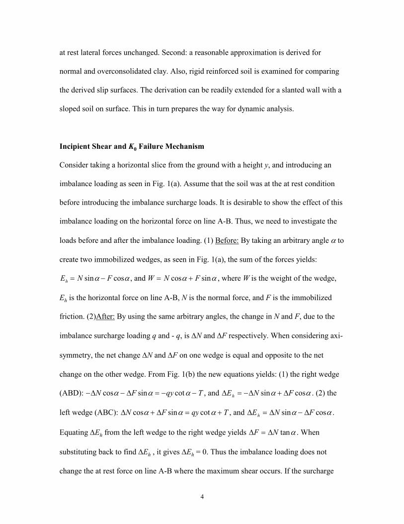
Consider taking a horizontal slice from the ground with a height y, and introducing an

imbalance loading as seen in Fig. 1(a). Assume that the soil was at the at rest condition

before introducing the imbalance surcharge loads. It is desirable to show the effect of this

imbalance loading on the horizontal force on line A-B. Thus, we need to investigate the

loads before and after the imbalance loading. (1) Before: By taking an arbitrary angle α to

create two immobilized wedges, as seen in Fig. 1(a), the sum of the forces yields:

E N Fh = −sin cosα α , and W N F= +cos sinα α , where W is the weight of the wedge,

Eh is the horizontal force on line A-B, N is the normal force, and F is the immobilized

friction. (2)After: By using the same arbitrary angles, the change in N and F, due to the

imbalance surcharge loading q and - q, is ∆N and ∆F respectively. When considering axi-

symmetry, the net change ∆N and ∆F on one wedge is equal and opposite to the net

change on the other wedge. From Fig. 1(b) the new equations yields: (1) the right wedge

(ABD): − − = − −∆ ∆N F qy Tcos sin cotα α α , and ∆ ∆ ∆E N Fh = − +sin cosα α . (2) the

left wedge (ABC): ∆ ∆N F qy Tcos sin cotα α α+ = + , and ∆ ∆ ∆E N Fh = −sin cosα α .

Equating ∆Eh from the left wedge to the right wedge yields ∆ ∆F N= tanα . When

substituting back to find ∆Eh , it gives ∆Eh = 0. Thus the imbalance loading does not

change the at rest force on line A-B where the maximum shear occurs. If the surcharge

5

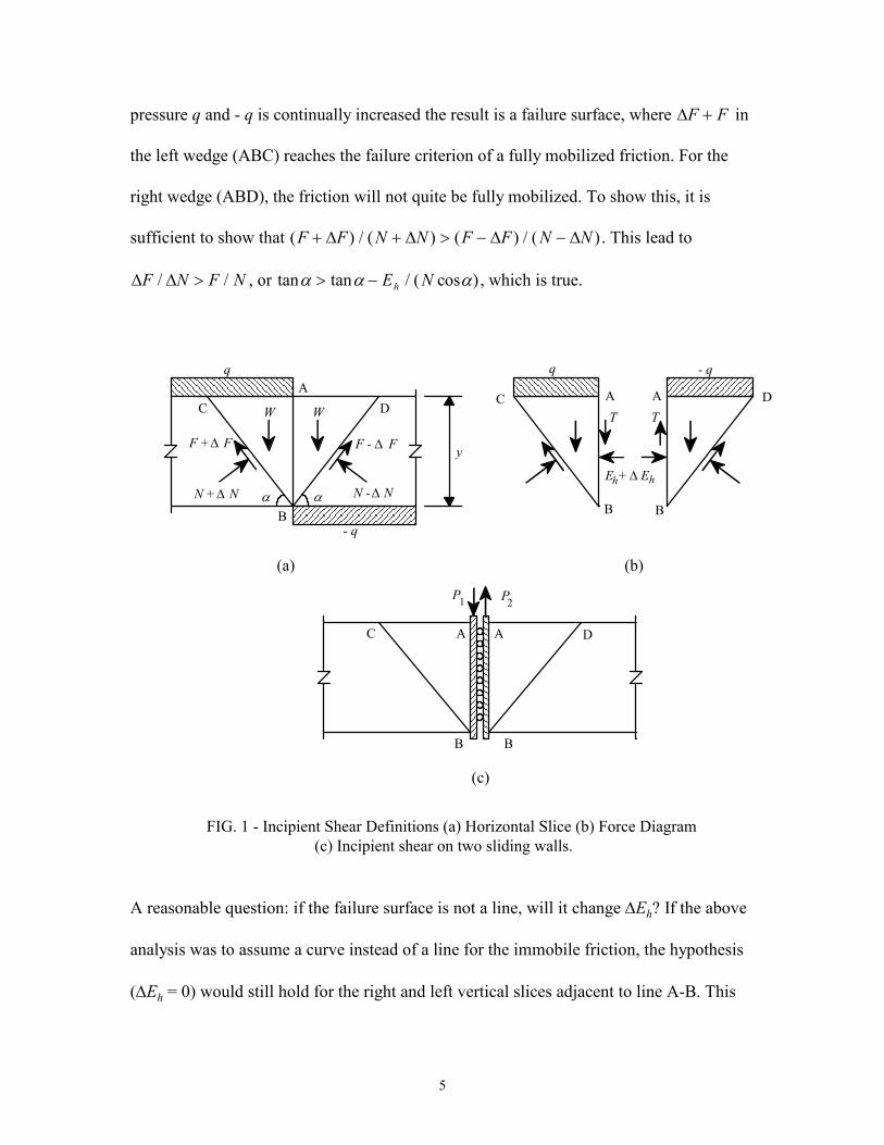
pressure q and - q is continually increased the result is a failure surface, where ∆F F+ in

the left wedge (ABC) reaches the failure criterion of a fully mobilized friction. For the

right wedge (ABD), the friction will not quite be fully mobilized. To show this, it is

sufficient to show that ( ) / ( ) ( ) / ( )F F N N F F N N+ + > − −∆ ∆ ∆ ∆ . This lead to

∆ ∆F N F N/ /> , or tan tan / ( cos )α α α> − E Nh , which is true.

N + N

F + F

∆

∆

∆∆

∆F - F

N - N

W W

y

E Ehh+

T T

q

- q

A

B

C DA A

B B

C D

q - q

P P1 2

A A

B B

C D

(a) (b)

(c)

FIG. 1 - Incipient Shear Definitions (a) Horizontal Slice (b) Force Diagram

(c) Incipient shear on two sliding walls.

α α

A reasonable question: if the failure surface is not a line, will it change ∆Eh? If the above

analysis was to assume a curve instead of a line for the immobile friction, the hypothesis

(∆Eh = 0) would still hold for the right and left vertical slices adjacent to line A-B. This

6

can be seen by treating the bottom of each slice as a wedge with some slope and a

surcharge on top of it. Repeating the analysis on each slice with its corresponding mirror

image slice, will give the same results, when summing all the forces. Thus, the hypothesis

is valid for any arbitrary curve, and not just a line. Furthermore, if the imbalance loading

q and - q were any axi-symmetric loading, the hypothesis that ∆Eh = 0 remains valid.

From this observation it is necessary to introduce a name for the type of shear, T, which

was introduced on line A-B to be the incipient shear. The full definition of the incipient

shear is: A shear introduced to a boundary or a line is an incipient shear when the

normal forces to the boundary or the line do not change. It is important to note that the

horizontal force of Fig. 1(a) does not need to be the at rest force. Thus, the incipient shear

hypothesis is applicable for other conditions.

It is noteworthy that the hypothesis of the incipient shear was arrived at without the use of

elasticity, plasticity, or elastoplastic methods. When comparing with elasticity the result is

the same. For example, integrating Flamant's equation, (1892) [27], for any axi-

symmetric load on a semi-infinite media yields σh = σv = 0, and the strain is zero at line

A-B of Fig. 1(a).

To simplify the analysis it would be beneficial not to deal with the surcharge q. Consider

the two buried walls in the horizontal slice of Fig. 1(c). Between the walls are rollers to

give a perfectly smooth surface. If P1 = P2, the wedge analysis is identical to the above for

Fig. 1(a). The result is the same hypothesis ∆Eh = 0. The first failure surface would be

that of P1, a downward incipient shear. The failure surface is expected to be different than

7

that of Fig. 1(a). However, the before and after, at rest lateral forces are kept the same

since ∆Eh = 0.

From these observations, when considering the downward incipient shear of Fig. 1(c), it

is expected that the K value will have variation inside the wall. It will start at K = K0 at

the wall and will reoccur internally at some distance inside the wall. This is necessary

since going further inside the wall, the incipient shear has a lesser influence on the

stresses and the at rest forces will reoccur. Thus K0 will reoccur at some point at x = xm

from the wall and the boundary condition on the slip surface can be considered to have K0

at both ends.

Once the K0 failure mechanism is realized, K0 can be derived from finding the maximum

horizontal force for an active slip surface. Additionally, the boundary condition must be

satisfied. Maximizing the horizontal force will lead to K0, and not any other active force

coefficient because the horizontal force will reduce if the boundary moves slightly

outward from zero deformation to an active slip surface. Experiments by Terzaghi (1934,

1941) [25, 26], Sherif et al. (1982,1984) [21, 23], and Fang et al. (1986) [7] indicated that

regardless of the outward movement of a rigid wall, the horizontal force reduces from the

at rest condition. Thus, the at rest force is the upper bound for an active slip surface

failure. These tests were done for translating walls, rotating walls from top and bottom.

The outward movement reduces the horizontal force from the at rest condition because it

induces tension in the soil. Cohesionless soil can hardly take tension. Thus, if the failing

wedge is subdivided into vertical slices, the shear in the slices will reduce. Excessive

8

outward movement will result in an active condition where the shear in the slices

becomes zero. Hence, it is sufficient to find the at rest force by maximization with an

active slip surface due to a downward incipient shear with the proper boundary condition.

Thus the necessary criterion in deriving K0 is obtained.

Boundary Conditions for Sand

Subdividing the failure wedge of the downward incipient shear into vertical slices,

following Bishop (1955) [1], yields slices that are each in equilibrium, so that the

overturning moments remain in balance and not of concern. Each slice is added together

to make the wedge in Fig. 2. The resultant of the boundary forces on a slice can be

transformed to a Coulomb, (1776) [3], wedge as shown on Fig. 3(a),(b). From the

Coulomb wedge one can write

( )( )dE

dwx =

−

+ −

tan

tan tan tan

α φ

α φ α1 δδδδ ,.............................................................................. (2)

( )dW

y dy y dy dw= −

− +

=γ

α α2 tan tan ,.......................................................................... (3)

dE dEy x= tanδδδδ ,......................................................................................................... (4)

and

dy dx= − tanα ............................................................................................................. (5)

Extremizing the boundary forces in a slice can be done in three ways: (1) extremizing the

horizontal force dEx , (2) extremizing the vertical force dEy , (3) extremizing the resultant

9

force of dEx and dEy. To extremize dEx it is necessary to hold dy constant and vary dx

because dEx = −Kydy, and extremizing K is of interest. Thus ydy must be

E E

y

x

y

x

x

y

0

−δ

−δ

π/4+φ/2

Second Slip Surface

First Slip Surface

FIG. 2- Slip Surfaces Due To Incipient Shear

n

n

m

m

n

n

m

m

π/4+φ/2

−δ

E0

0

(0,y )0

10

dxdx

y-dy

dy

dQ dQ

dW

dW

dE

dE

E

E

E

E

x

y

i

ii

i

i+1

i+1

i+1

i+1

cos

cos

sin

sinδ

δ

δ

δ

δδδδ

αα

φφ

α−φα−φ

δ

δi+1

i

FIG. 3-a Bishop Slice FIG. 3-b Coulomb Wedge

held constant. To extremize dEy dx must be held constant and dy must be varied. dEy

must be extremized to achieve a constant dW = γydx. Thus, ydx must remain constant. In

many cases, dEy is taken as dE x tanδδδδ . In these cases dy is to be held constant and dx is to

vary. To extremize the resultant it requires dx tan( ) / cosα − δδδδ δδδδ be held constant. This can

be realized by rotating the axis by δδδδ from the vertical in order to have the resultant in a

horizontal direction.

In the boundaries in Fig. 2, it is desirable to find the angle α that gives the smallest dEy,

which causes the first and last slice to fail, while dEx is at maximum. From the above

consideration on extremizing the forces in a slice, one finds that dx and dy must be held

constant. This gives no unique solution since two different α's can be derived from Eq. 5.

However, at the boundaries the forces are already at maximum and dEx = K0γydy

11

regardless of α or the value of the incipient shear. Additionally, the bulk of the movement

is in the vertical direction. Thus the failure of these slices will be primarily from dEy due

to the incipient shear. Therefore the slice wedge at the boundaries can be considered to

have movements in the vertical direction, and α can be obtained by keeping only dx

constant. Writing Eq. 2 in terms of dEx and dEy with Eq. 5 and Eq. 3, yields

[ ]− = −

− ++ − = − + −dE

y dy ydx dE ydx K ydxy xγ α φ γ γ α α φ

( )cot( ) ( ) tan cot( )

2 0 ........ (6)

Minimizing the downward force -dEy in Eq. 6, − == =

dE

d

y

x x xmα

0

0 and

, yields

α α α π φ= = = +0 4 2m / / .......................................................................................... (7)

where α0 is the wedge angle for the first slice, and αm is for the last slice. Note: α = 0 is

not considered as solution for the minimum of Eq. 6, since the downward movement will

cause a non-zero slope in the slices. Also, α π φ= +/ 2 cannot be considered as a solution

since α π≤ / 2. Now that the boundary conditions are selected, maximizing the horizontal

force with these boundaries must result in K0. A first approximation can be done by

selecting the slip surface as a line with a slope at all α's in the slices to be π φ/ /4 2+ ,

and selecting δδδδ = −φ to maximize the horizontal force in Eq. 2. Substituting

α π φ= +/ /4 2 , and δδδδ = −φ in Eq. 2 and integrating y from y0 to zero yields

E dE ydyx y0 0

0 4 2

1 4 2

1

4 20

costan( / / )

tan tan( / / ) tan( / / )δ γ

π φφ π φ π φ

= ≅ −−

− − +∫∫

12

≅ −γ

φy0

2

21( sin ) .............................................................................. (8)

where the identity tan( / / ) tan / cosπ φ φ φ4 2 1± = ± + were used. Eq. 8 gives a

K0 1≅ − sinφ as in Eq. 1, where Jáky's equation is derived from unacceptable

assumptions and is considered a coincidence. There are considerations that need to be

investigated for this approximation: (1) The integration of Eq. 4 yields δ0 = −φ. However,

another slip surface can occur before this one, where the incipient shear is lower and

reaches a directional angle −δ0 < φ with a slightly higher K0 value than Eq. 8. This will be

shown later on in the derivation. (2) Eq. 8 is derived by assuming a constant K0 value in

all the slices. This is contrary to common sense since variation in the stresses, thus the K

value, are expected inside the wall. It can be concluded that Eq. 8 or Jáky's equation is

only an approximation, and the slip surface and the directional angle δ0 are incorrect.

Sand Analysis

K0 for sand will be derived from an extremum condition using variational methods with

the boundary condition of Eq. 7. With the extremum method one selects arbitrary

admissible slip surfaces and determines the forces acting on the boundaries of the earth

mass. The definitive slip surface is one, which furnishes an extremum value for the

horizontal force. Maximizing the horizontal force E0 0cosδ can start by maximizing each

slice individually. The horizontal force dEx of the slice in Eq. 2 can be treated as a

coulomb wedge with a uniform surcharge; it is required that dE

d

x

α= 0 . Thus

13

( ) ( )( )

( )( )

( )tan

sin

sin tan

cos sin

sin

cot cot cot

cot cotδδδδ =

−−

−=

−

−=

− +

−

2

21

1 2 1 22

2

2

α

α φ α φ

α φ φ

α φ

α φ α

φ α

............................................................................................................. (9)

where tanδδδδ is expressed three different ways for convenience and it yields

( ) ( )[ ]cot tan cot cotα φ φ φ= − + − + +δδδδ δδδδ1 1 .............................................................. (10)

If plotting Eq. 10 it shows that α > φ for all −φ ≤ δδδδ ≤ φ. Also, Eq.10 is the Coulomb

wedge angle for a vertical wall with wall friction. If δδδδ = 0 in Eq. 9 or 10 α =

π/4 + φ/2, where ( )− + = +tan / cos cot / /φ φ π φ1 4 2 . This checks with an active

Coulomb wedge with δδδδ = 0 . Now, note for α > φ in Eq. 2 the force dEx is maximized

when δδδδ ≤ 0. Thus the boundary points for the slip surface of Fig. 2 can be taken in the

region −φ ≤ δδδδ ≤ 0 or at π/4 + φ/2 ≤ α ≤ π/2. Thus, α0 = π/4 + φ/2 , and αn= π/2 as in Eq. 7.

For a given y0, xn and yn will be determined from these prescribed end points. Substituting

Eq. 9 in Eq. 2 and 4 and rearranging yields

( )dE ydxx = −γ φ φ α αsin cot cot tan2 2 ...................................................................... (11)

( )dE ydx ydxy = + −2 2γ φ γ φ φ α αsin sin cos cot tan

( )= − + +γ φ α γ φ φ φ α αtan tan cos sin tan cot tanydx ydx2

( )= −tan cotφ γ αydx dEx ................................................................................... (12)

Where dw

tanα is replaced by γydx, γ is the soil constant, and dEy is expressed in different

ways for convenience. From Fig. 3a one can write

14

E E dEi i i i xcos cosδ δ− =+ +1 1 ..................................................................................... (13)

E E dEi i i i ysin sinδ δ− =+ +1 1 ...................................................................................... (14)

When starting with E0 and ending with En Eqs. 13 and 14 yields

E dE Exi

n

n n0 00

1

cos cosδ δ= +=

−

∑ .................................................................................... (15)

E dE Eyi

n

n n0 00

1

sin sinδ δ= +=

−

∑ ..................................................................................... (16)

By taking tanα = − ′y in Eq. 11 and 12 and replacing the summation sign by the integral

sign in Eq. 15 and 16 it yields

Ey

y ydx Ex

n n

n

0 0

2

0

21

cos sin cot cosδ γ φ φ δ= − +′

′ +∫ ................................................ (17)

E ydx yy

ydx Ex

n n

xn n

0 0

2

0 02

1sin sin sin cos sinδ γ φ γ φ φ δ= + ′−

′

+∫ ∫

= ′ − −′

′ +∫∫γ φ γ φ φ φ δtan sin cos tan siny ydx

yy ydx En n

xx nn 12

00

= −′

− +∫∫γ φ γ φ δtan tan siny

ydx dE Ex

xx

n n

nn

00 ........................................... (18)

To use variational method to maximize horizontal force E0 0cosδ , Eq. 17 needs to be

extremized while Eq. 18 is to be satisfied. Eq. 18 can be satisfied by choosing the proper

15

directional angles δ0 and δn. Similarly, E0 0cosδ can be maximized by extremizing Eq. 18

while Eq. 17 to be satisfied, and again the proper directional angles can satisfy Eq. 17.

Note: E0 0sinδ is taken as ( cos ) tanE0 0 0δ δ . These conditions leads to a deduction that

there are two slip surfaces that can maximize E0 0cosδ , and both surfaces can occur.

Since it is desirable to look for the horizontal pressure in Fig. 2, the resulting slip surface

from maximizing Eq. 17 will be the first slip surface and the slip surface resulting from

maximizing Eq. 18 will be the next one. This situation will become more evident when

the slip surfaces are obtained and the boundary conditions are imposed. Thus, Eq. 17 or

18 can be extremized alone while the other can be satisfied with a suitable δ0 and δn.

When starting with Eq. 17 the boundary conditions are prescribed: at x = 0 y = y0, at x = 0

and y = y0 ( )′ = − − = −x tan / / tan / cosπ φ φ φ4 2 1 , and at x = xn and y = yn ′x = 0. Note

also that En ncosδ in Eq. 17 is prescribed from a second slip surface such that

δ( cos )En nδ = 0. Thus, the Euler equation [29] from variational method can be applied:

∂∂

∂∂

ℜ−

ℜ

′

=

y

d

dx y0 ..................................................................................................... (19)

where ℜ = − +′

′γ φ φsin cot2

21

yy y ......................................................................... (20)

Since ℜ does not involve x explicitly then

ℜ− ′ℜ

′=y

yh

∂∂

............................................................................................................ (21)

where h is a constant. Applying Eq. 21 on Eq. 20 yields

16

11

′= − −

y

h

ycot

'φ .................................................................................................... (22)

where h' is a new constant. By using the boundary condition ′ =x 0 at y yn= , h' can be

found and Eq. 22 can be written as

11

′= ′ = − −

yx

y

y

ncot φ ........................................................................................... (23)

By using the end condition at y y x= ′ = − = +0 01 4 2 for tan / cos / /φ φ α π φ on Eq.

23 yields

( )y yn0 1= + sinφ ....................................................................................................... (24)

When integrating Eq. 23 and using the end condition at x y y= =0 0 , it yields the first

slip surface Eq.:

x y y yy

yn= − − −

cot lnφ 0

0

.................................................................................... (25)

By using Eq. 24, Eq. 25 can be written as

( )( )[ ]Ω =+

− + − +cot

sinsin ln

φφ

φ ψ ψ1

1 1 ...................................................................... (26)

Where Ω = =x

y

y

y0 0

and ψ . Fig. 4 shows different slip surfaces for various values of φ

for the region 1

11

+< <

sinφψ . The horizontal distance can be written as

[ ]xy

n = ++ +0

11

cot

sinsin ln( sin )

φφ

φ φ .............................................................................. (27)

17

0.2

0.3

0.4

0.5

0.6

0.7

0.8

0.9

1

1.1

0 0.05 0.1 0.15 0.2 0.25

ψ

Ω

φ=20

φ=30φ=40

FIG. 4 K0 First Slip Surface

By substituting Eq. 23 in Eq. 17 and 18, changing the interval to [ , ]y yn0 instead of

[ , ]0 xn , and replacing ′y dx by dy, yields

Ey

ydy E

n

y

y

n n

n

0 0

2

2 2

0

cos sincot

cosδ γ φφ

δ= − +∫

= +γ φ δyy

yEn

n

n n

2 2 0cos ln cos ................................................................... (28)

( )( )E y y y y yy

yEn n n

n

n n0 0 0 0

2 2 0

23sin

cotcot cos ln sinδ

γ φγ φ φ δ= − − + + .................. (29)

18

Substituting Eq. 24 in Eq. 28 and 29 yields

( )E y En n n0 0

2 2 1cos cos ln sin cosδ γ φ φ δ= + + ............................................................ (30)

( ) ( )Ey

y En

n n n0 0

2

2 2

22 1sin

cossin cot cos ln sin sinδ γ

φφ γ φ φ φ δ= − − + + + ............... (31)

Thus the analysis of the first slip surface is obtained. Note for x xn> Eq. 23 has no y

values. In fact the curve circles toward the first boundary, as seen in Fig. 2, indicating

another slip surface must occur in order to reach the top of the ground. So, it remains to

find the second slip surface and the force En . Consider the second slip surface shown in

Fig. 2.

For maximum condition in the slice using Eq. 2 and for matching the end of the first slip

surface, the boundary condition can be taken as α π α π φn m= = +/ / /2 4 2 and .

Rewriting Eq. 17 and 18 in terms of the forces of the second slip surface in Fig. 2, yields

Ey

y ydx En n m mx

x

n

m

cos sin cot cosδ γ φ φ δ= − +′

′ +∫2

21

.............................................. (32)

E y ydxy

y ydx En n x

x

x

x

m mn

m

n

m

sin tan sin cos tan sinδ γ φ γ φ φ φ δ= ′ − −′

′ +∫ ∫ 12

................. (33)

Using variational method on Eq. 33 to extremize En ncosδ yields

′ = −

x

h

ytan

'φ 1 ........................................................................................................ (34)

19

where h' is a constant. By using the boundary condition at y y x yn= ′ = ′ = 1 0/ for

α πn = / 2 on Eq. 34, h' is found and the equation can be rewritten as

′ = −

x

y

y

ntanφ 1 ...................................................................................................... (35)

Using the other end condition at y y xm= ′ = − tan / cosφ φ1 for α π φm = +/ /4 2 , Eq.

35 yields

y ym n= sinφ ............................................................................................................. (36)

When integrating Eq. 35 and using the end condition at x x y yn n= = , the second slip

surface is obtained:

x y y yy

yxn n

n

n= − −

+tan lnφ ................................................................................ (37)

From Eq. 24, 27 and 36, Eq. 37 can be rewritten as

[ ][ ] [ ] Ω =+

+ − − + + − +1

11 1 1 1

sintan ( sin ) ln ( sin ) cot sin ln( sin )

φφ φ ψ φ ψ φ φ φ ........ (38)

Where Ω = =x

y

y

y0 0

, , and sin

1+ sin< <

1

1+ sin,ψ

φφ

ψφ

see Fig. 4 for the plot of Ω and

ψ for the second slip surface. The total horizontal distance can be written as

[ ] [ ] xy

m =+

− − + − +0

11 1

sintan sin ln(sin ) cot sin ln( sin )

φφ φ φ φ φ φ .......................... (39)

20

By substituting Eq. 35 in Eq. 32 and 33 with the interval [yn, ym] instead of [xn, xm] and

with ′ =y dx dy , it yields

E yy

y

y

y

y

yEn n n

m

n

m

n

m

n

m ncoscos

tan tan sin ln cosδ γφ

φ φ φ δ= −

− −

−

+2

2

2

2 2 21

21 2 1

.............................................................................................. (40)

E yy

y

y

yEn n n

m

n

m

n

m msintan

tan sin ln sinδ γφ

φ φ δ= − −

−

+2

2

2

21 ......................... (41)

Substituting Eq. 36 in Eq. 40 and 41 yields

( ) ( )E y En n n m mcos tan sin tan sin ln sin cosδ γ φ φ φ φ φ δ= − − −

+2 2 2 2

1

22 1 ................ (42)

( )E y En n n m msinsin cos

tan sin ln sin sinδ γφ φ

φ φ φ δ= − +

+2 2

2 ................................. (43)

Substituting Eq. 42 and 43 in Eq. 30 and 31 yields

( ) ( ) ( )E y En m m0 0

2 2 2 2 21

1

22 1cos cos ln sin tan sin tan sin ln sin cosδ γ φ φ φ φ φ φ φ δ= + + − − −

+

............................................................................................ (44)

( ) ( ) ( )E y En m m0 0

2 2 2

22 1

2sin

cossin cot cos ln sin

sin costan sin ln sin sinδ γ

φφ φ φ φ

φ φφ φ φ δ= − − + + − −

+

............................................................................................ (45)

21

Now Eq. 44 and 45 gives the maximum possible E0 0cosδ for the given boundary

conditions. Since the boundary conditions are satisfied, the horizontal forces can be taken

as E Ky

E Ky

m m

m

0 0 0

0

2

0

2

2 2cos cosδ γ δ γ= = , and in Eq. 44. Thus, from Eq. 44, 24, and

36 K0 can be found:

( ) ( ) ( )( )

K0

2 2 2 2

2 2

2 1 1 4 1 2

1=

+ + − − −

+ −

cos ln sin sin tan tan sin ln sin

sin sin

φ φ φ φ φ φ φ

φ φ .................. (46)

Since δ δ0 and m are arbitrary, they can be set equal. This can be realized since the

incipient shear can be assumed to vary linearly with depth at the boundaries. Thus, from

Eq. 45, setting E E Ky

0 0 0 0 0 0

0

2

02sin cos tan tanδ δ δ γ δ= = and

E E Ky

m m m m

msin cos tanδ δ γ δ= = 0

2

02, it yields the incipient shear directional angle:

( ) ( ) ( )( )[ ]

tan tancos sin cot cos ln sin sin cos tan sin ln sin

sin sinδ δ

φ φ φ φ φ φ φ φ φ φ

φ φ0

2 2

2 2

0

2 2 1 2

1= =

− − + + − −

+ −m

K

.................................................................................................... (47)

From Eq. 30 and 31 tanδ n can be expressed as:

( ) ( )( )tan

sin cos sin / cot cos ln sin

cos cos ln sinδ

δ γ φ φ γ φ φ φ

δ γ φ φn

n n

n

E y y

E y=

+ − − +

− +0 0

2 2 2

0 0

2 2

2 2 1

1 ................... (48)

or

( ) ( ) ( )( ) ( )

tansin tan cos sin cot cos ln sin

sin cos ln sinδ

φ δ φ φ φ φ φ

φ φ φn

K

K=

+ + − − +

+ − +

0

2

0

2

0

2 2

1 2 2 1

1 2 1 .................. (49)

22

Table 1 gives the comparison of different K0 for Jáky, Handy, and as derived. Note

− <δ φ0 for all φ and the incipient shear is smaller indicating that K0 of Eq. 46 supersedes

that of Eq. 8.

Due to the propagation of the incipient shear, it can be anticipated that the two slip

surfaces can repeat for x xm> . Now, it is important to show that the K0 of Eq. 46 is the

same when considering all the slip surfaces to the top of the ground. Let K1 be the term in

the bracket of Eq. 44. Utilizing Eqs. 24 and 36, an expression from one set of slip

surfaces to another can be obtained: y yn n( ) / ( ) sin / ( sin )bot top = +φ φ1 . Using this

relation and substituting all sets of slip surfaces in Eq. 44 yields

E K yn0 0 1

2

2 4 6

11 1 1

cossin

sin

sin

sin

sin

sinδ γ

φφ

φφ

φφ

= ++

+

+

+

+

+ ⋅ ⋅ ⋅ ⋅ ⋅ ⋅........................ (50)

or

( )E K y

K y K yn

i

i

n

0 0 1

2

2

0

1

2 2

2 2

0 0

2

1

1

1 2cos

sin

sin

sin

( sin ) sinδ γ

φφ

γ φφ φ

γ=

+

=

+

+ −=

=

∞

∑ .............................. (51)

This gives exactly the same K0 of Eq. 46. Thus, the solution is consistent, and this method

of substitution can also be done on Eq. 45 to show that tanδ 0 is exactly the same as that

of Eq. 47. Consequently, the assumption that δ δ0 = m is correct.

23

φ Jáky Jáky Handy Handy Derived δ0 = δm* δn*

Deg. 1-sinφ 0.9-sinφ 1.1(1-sinφ) 1.06(1-sinφ) K0 Deg. Deg.

***0 1.0000 0.9000 1.1000 1.0600 1.0000 0.00 -0.00

10 0.8264 0.7264 0.9090 0.8759 0.8989 -8.90 -9.58

20 0.6580 0.5580 0.7238 0.6975 0.7150 -16.67 -18.37

30 0.5000 0.4000 0.5500 0.5300 0.5285 -24.36 -26.74

40 0.3572 0.2572 0.3929 0.3786 0.3648 -32.51 -35.06

50 0.2340 0.1340 0.2574 0.2480 0.2311 -41.54 -43.72

60 0.1340 0.0340 0.1474 0.1420 0.1287 -51.77 -53.18

70 0.0603 -0.0397 0.0663 0.0639 0.0567 -63.38 -63.97

80 0.0152 -0.0848 0.0167 0.0161 0.0141 -76.29 -76.38

**90 0.0000 -0.1000 0.0000 0.0000 0.0000 -90.00 -90.00

* Derived in this paper. ** As in completely rigid. *** As in hydrostatic.

Table 1- K0 comparison

Comparing K0 sand with experiments

Mayne and Kulhawy, (1982) [17], made a statistical analysis of 171 tests, where some of

these tests had missing φ values (some in clay and some in sand). Their result showed that

Jáky's equation is applicable. However, the linear regression was biased toward curve

fitting Jáky's equation. Their correlation number r = 0.802 for 121 points. Adding 17

24

more tests, see reference [ 4, 5, 6, 15, 16, 18, 19, 20], and computing the absolute value of

the error on 138 tests yields:

Error Derived Jáky

0 to 1% 23 18

1 to 5% 58 70

5 to 16% 57 50

Total No. of tests 138 138

It is clear from this observation that the derived K0 compares with experiments just as

good, perhaps a little better.

Comparison of the slip surface for sand with experiments

There is no available experimental data publication on slip surfaces for K0 due to shear

failure. However, it is notable that the slip surfaces are similar results to slip surfaces of

rigid reinforced earth problems. In the reinforced soil walls (rigid type), the developments

of the force E E0 0 0 0cos sinδ δ and are dissipated in the reinforcements. Thus dEx and

dEy in every slice are reduced by the tension of each segment in the reinforcements,

ending with E0 = 0 at the face of the wall. The problem of maximization has the same

equations as the rigid wall. In this case, the forces in the reinforcements need to be

maximized instead of the force on the boundaries. Thus, ∑dEx and ∑dEy needs to be

maximized, where the slice of Fig. 3(a) and (b) will have reinforcements sticking out of it

and dEx and dEy represent the resultant forces. Thus, the resulting slip surface must be the

25

same as the derived ones. Also, the boundary conditions on the slip surface are the same.

Experimentally α0 = π/4 + φ/2 , see Juran and Christopher, (1989) [13]. Thus, from the

first slip surface in Eq. 28 and 29, −δn will have higher values than φ, since δ 0 0= . This

is expected since the shear can be taken by the reinforcements. The second slip surface

will finish at a point similar to the front face, since that portion of the wall can be taken as

a surcharge on a layer of reinforcements. Thus the tension in these reinforcements takes

the lateral load leaving the upper surface at the surcharge area to start anew. Thus,

α π φm = +/ /4 2 . At this point δm will have a value similar to δn. Thus, from there on it

can be considered similar to an incipient shear at zero deflection, and the slip surfaces

will repeat. When integrating over all the slip surfaces, the final horizontal and vertical

forces to the top of the wall will not be zero; they represent the total horizontal and

vertical forces in the reinforcements. In both cases, the friction on the bottom of the slices

is fully mobilized causing an active slip surface. Even though the equations come out the

same, due to the variational function, the location of the forces are not in the same place.

To find the location of ∑dEx and ∑dEy in a reinforced earth mass, it is necessary to take

moments of the slices. Thus Mx = ∑ydEx and My = ∑xdEy. By integrating over all the slip

surfaces, to the top of ground, the moments can be obtained, thus the location of the

forces.

When comparing with an experiment found by Juran, Beech, and De Laure[12] this gives

a good result. Their experiment gave data for a slip surface for a rigid inclusion

26

0.1

0.2

0.3

0.4

0.5

0.6

0.7

0.8

0.9

1

1.1

0 0.05 0.1 0.15 0.2 0.25

Z/H=y/y0

S/H = x/y0

O = Experimental___ = Equation 26 & 38

O

O

O

O

O

O

O

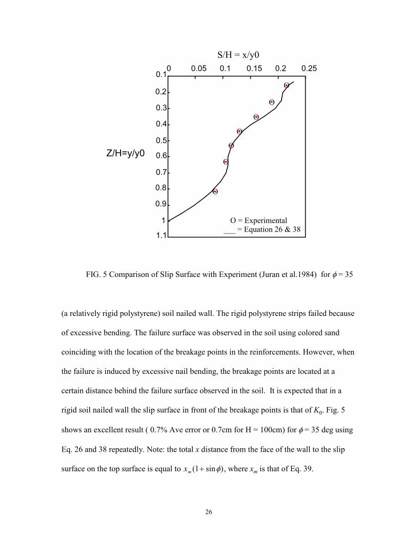
FIG. 5 Comparison of Slip Surface with Experiment (Juran et al.1984) for φ = 35

(a relatively rigid polystyrene) soil nailed wall. The rigid polystyrene strips failed because

of excessive bending. The failure surface was observed in the soil using colored sand

coinciding with the location of the breakage points in the reinforcements. However, when

the failure is induced by excessive nail bending, the breakage points are located at a

certain distance behind the failure surface observed in the soil. It is expected that in a

rigid soil nailed wall the slip surface in front of the breakage points is that of K0. Fig. 5

shows an excellent result ( 0.7% Ave error or 0.7cm for H = 100cm) for φ = 35 deg using

Eq. 26 and 38 repeatedly. Note: the total x distance from the face of the wall to the slip

surface on the top surface is equal to xm ( sin )1+ φ , where xm is that of Eq. 39.

27

0

10

20

30

40

50

60

70

80

90

0 5 10 15 20 25

H=y - cm

D=x - cm

O = Experimental___ = Equation 25 & 37

OO

O

O

O

O

OO

OO

OO

FIG. 6 Comparison of Slip Surface with Experiment (Juran et al. 1989)

(Model No. 3 - End of Construction) φ = 40 and y0 = 80 cm

Juran and Christopher[13] did a laboratory model study on geosynthetic reinforced soil

retaining walls. The soil used in the study was a fine Fontainbleau sand (poorly graded,

average grain diameter 0.1 mm) with φ = 40. Colored sand was used to detect the failure

surface in the soil. Three different types of geosynthetic reinforcing materials were used:

Woven polyester strips; non-woven geotextiles; and plastic grids. The results on the

tension forces measured in the woven geotextile strips correspond fairly well to those

estimated, assuming that the soil is at K0 state stress. In his third model wall (Model No.

3) the initial failure surface at end of construction was observed to be quite different from

28

0

10

20

30

40

50

60

70

0 5 10 15

H=y - cm

D=x - cm

O = Left Facing

∆ = Right Facing___ = Equation 25 & 37

O

O

∆

∆

∆

∆

O

O

O

O

∆

O

O

FIG. 7 Comparison of Slip Surface with Experiment (Juran et al. 1989)

(Model No. 7 - with Plastic Grids) φ = 40 and y0 = 59.5 cm

Coulomb's failure plane, whereas the final one (failure after 12hr) corresponds fairly well

to Coulomb's failure plane. It is expected that the initial failure surface at end of

construction will correspond to K0 failure surface. Fig. 6 shows an excellent result ( 1.3%

Ave error or 1.05cm for H = 80cm) for φ = 40 deg, where the angle φ = 40 gives the exact

Coulomb's failure plane observed after 12hr. The results on the tension forces measured

in the non-woven geotextiles for low overburden correspond fairly well to those

estimated, assuming that the soil is at Ka state stress. However, as the overburden stress

increases, the reinforcement material seems to undergo a strain hardening phenomenon

and the tension forces in the reinforcements approach those predicted, considering a K0

29

state of stress in the soil. The initial failure surface is expected to be of a K0 slip surface

but it was not recorded. However, it was mentioned in Juran, Ider, and Farrag[14] to be

an inclination of 75 to 78 degrees; which is expected for a K0. The result on the tension

forces measured in the plastic grid are close to those predicted, assuming that the soil is at

K0 state stress. The initial and final surface is quite different from the Coulomb failure

surface. This is expected since rigid inclusions were used. Fig. 7 shows excellent result (

1.12% Ave error or 0.66cm for H = 59.5cm) for φ = 40 deg.

Overconsolidation of sand

When the present effective overburden pressure is the maximum pressure to which the

soil has been subjected at any time in its history, the deposit is referred to as normally

consolidated. A soil deposit that has been fully consolidated under a pressure larger than

that of the present overburden is called overconsolidated. The K0 of Eq. 8 and 46 is

referred to as normal consolidation because the weight used in the derivation is the

existing weight, and no prehistoric weight causing locked-in stresses were used. To

achieve overconsolidation forces, locked-in horizontal forces must enter the equations

and be considered on each slice. For the purpose of demonstration of dependencies, a

one-dimensional approach will be used. Consider the structural beam in Fig. 8.

30

Removed Load q (y)0

P P

L−∆

Beam depth = Beam Thickness = dy dz

Beam Length = L

= Lock up Force = Axial Deflection∆P

E = Elastic Modulus of Beam

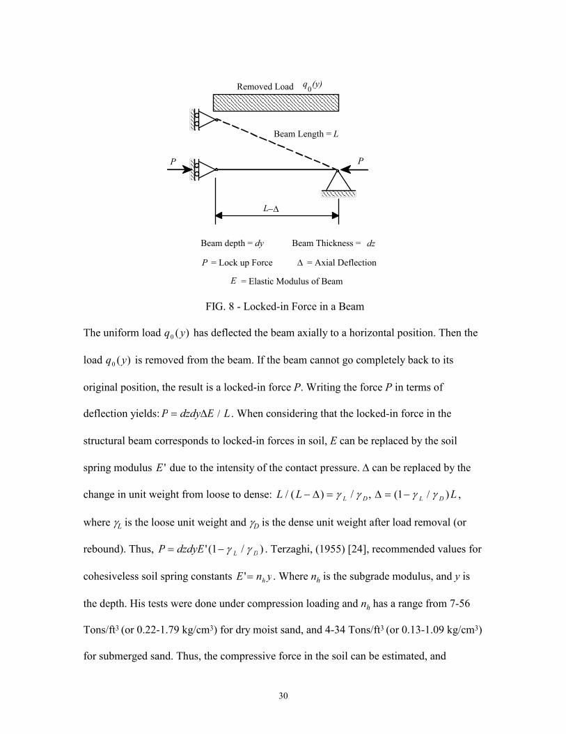
FIG. 8 - Locked-in Force in a Beam

The uniform load q y0 ( ) has deflected the beam axially to a horizontal position. Then the

load q y0 ( ) is removed from the beam. If the beam cannot go completely back to its

original position, the result is a locked-in force P. Writing the force P in terms of

deflection yields:P dzdy E L= ∆ / . When considering that the locked-in force in the

structural beam corresponds to locked-in forces in soil, E can be replaced by the soil

spring modulus E ' due to the intensity of the contact pressure. ∆ can be replaced by the

change in unit weight from loose to dense: L L L D/ ( ) /− =∆ γ γ , ∆ = −( / )1 γ γL D L ,

where γL is the loose unit weight and γD is the dense unit weight after load removal (or

rebound). Thus, P dzdyE L D= −' ( / )1 γ γ . Terzaghi, (1955) [24], recommended values for

cohesiveless soil spring constants E n yh'= . Where nh is the subgrade modulus, and y is

the depth. His tests were done under compression loading and nh has a range from 7-56

Tons/ft3 (or 0.22-1.79 kg/cm3) for dry moist sand, and 4-34 Tons/ft3 (or 0.13-1.09 kg/cm3)

for submerged sand. Thus, the compressive force in the soil can be estimated, and

31

P n ydzdycompressive h L D= −( / )1 γ γ . To find the necessary locked-in stresses to be used along

with the at rest forces, one must find the expansion force. Since soil is not elastic, the

compression force is not equal to the expansion force and it is much greater.

Consequently, the compression force can be reduced by using the expansion to

compression voids ratio. Thus the expansion locked-in force becomes

P ne e

e eydzdyh

e c

i c

L

D

expansion =−−

−

1

γγ

.............................................................................. (52)

So, ee is the expansion voids ratio at rebound or at load removal at γD, ec is the

compressed voids ratio at full load, and ei is the initial voids ratio at loose state γL. Now,

if the prehistoric surcharge is q yc ( ), then the compressive horizontal force is

K q y dydzc0 ( ) . However, not all of the surcharge can be used since some expansion in the

soil will occur after the removal of the surcharge. Thus, at compression to γD the

horizontal locked-in force can be taken as q(y)dydz, where q(y) is to be determined.

Equating this force with the expansion force of Eq. 52 yields

q y ne e

e eydyh

e c

i c

L

D

( ) =−−

−

1

γγ

..................................................................................... (53)

In order to include q(y) in the derivation, the forces must be split into loose condition plus

the locked-in force of Eq. 53. This is necessary since the estimated ∆ was for loose to

dense sand. Additionally, from Fig. 8, the overconsolidation force is to be considered

only in the horizontal direction. Thus, the resultant dE dEx y and for Eq. 2, 3, and 4

becomes:

32

dEdw

ne e

e eydyx h

e c

i c

L

D

=−

+ −+

−−

−

tan( )

tan tan( ) tan

α φα φ α

γγ1

1δδδδ

.............................................. (54)

dEdw

y =−

+ −tan( ) tan

tan tan( ) tan

α φα φ α

δδδδδδδδ1

................................................................................... (55)

( )dW

y dy y dy dwL= −

− +

=γ

α α2 tan tan......................................................................... (56)

When performing the boundary analysis, dEx in Eq. 6 must have the additional term in

Eq. 54, and so the resulting boundary condition remains the same. Furthermore, when

performing the same analysis for obtaining δδδδ and variational analysis the result leads to

the same slip surfaces. Therefore, the resulting coefficient K0c for over consolidation

becomes:

K Kn e e

e eK

n e e

e ec

h

L

e c

i c

L

D

h

D

e c

i c

D

L

0 0 01 1= +−−

−

= +

−−

−

γγγ γ

γγ

............................................ (57)

tan tanδ δ0

0

0

0c

c

K

K= .................................................................................................... (58)

Where, K0 is of Eq. 46 (with φ for loose sand), and δ0 is of Eq. 47 (with φ for loose sand).

It is remarkable that φ has no influence on the additive term due to overconsolidation, and

γL and γD has the greatest influence. Let k n e e e eh h D e c i c= − −( / )[( ) / ( )]γ . The term kh is

approximately constant, since nh is obtained by similar methods as the expansion to

compression deflection ratio. nh varies with the density of material, and so are the

required voids ratios. The variation of γD from γL is in the range from 0 to 6%. So, γD can

be considered approximately constant. Thus, the term kh can be considered constant. On

33

the other hand, the incipient shear angle is reduced per Eq. 58. This is expected, since the

failure wedge will be reached sooner due to overconsolidation. It is important to keep in

mind that Eq. 57 and Eq. 58 were derived to investigate dependencies for a very complex

problem. However, it is of merit to compare with experimental results. Sherif et. al.,

(1985) [22], showed that the variation of the additional term to K0(loose) is linearly

dependent with γD/γL . Their experimental results for dry Ottowa Sand gave the value for

kh = 5.5. When using an average value nh = 27 tcf and γD = 100 pcf (from Sherif et. al.) it

yields ( ) / ( ) . / .e e e ee c i c− − = =55 540 001. This is a very reasonable expansion to

compression deflection ratio in sand. Thus it appears that Eq. 57 and 58 are valid for the

conditions described above. When repeating the analysis in a higher dimension, as in a

circular plate or a square plate with plane strain analysis, new equations can be derived.

Thus, P = dzdy∆E/[L(1+ν)(1−2ν)], where ν is Poisson's ratio. From the volume ratio of

before and after, ∆ / /L L D= −1 γ γ giving [ ]K Kc D L D L0 0 10 6= + −. / /γ γ γ γ , where

ν was replaced by .3 for sand and kh = 5.5 (from Sherif et. al.). When comparing

numerically this equation with Sherif 's equation the results is of no significance in the

difference in the additive term to K0 where 1 107< <γ γD L/ . .

Clay Analysis

Preliminary analysis indicates when the cohesion "c" is involved in the equations,

mathematical harmony is difficult to achieve. It indicates that c will influence the slip

34

surfaces, K0, and the incipient shear angle. If the solution is to be done for only cohesion

with φ = 0, the boundary angle becomes 45 degrees, and the variational equation gives a

45 degrees line as the slip surface. This is an indication that if cohesion is added it will

influence the solution more toward a line than a curve. Thus, a reasonable approximation

of the solution for the normal consolidating clay can be obtained by using similar

procedures as in Eq. 8. Table 1 shows the difference between Eq. 8 (Jáky's Eq. 1) and the

derived Eq. 46 ranges from 0 to 8%. This difference can always be handled with a safety

factor similar to the one proposed by Handy, (1985) [8]. When adding the cohesion c on

the bottom of the slice, while keeping it in an upward direction and separate from dQ in

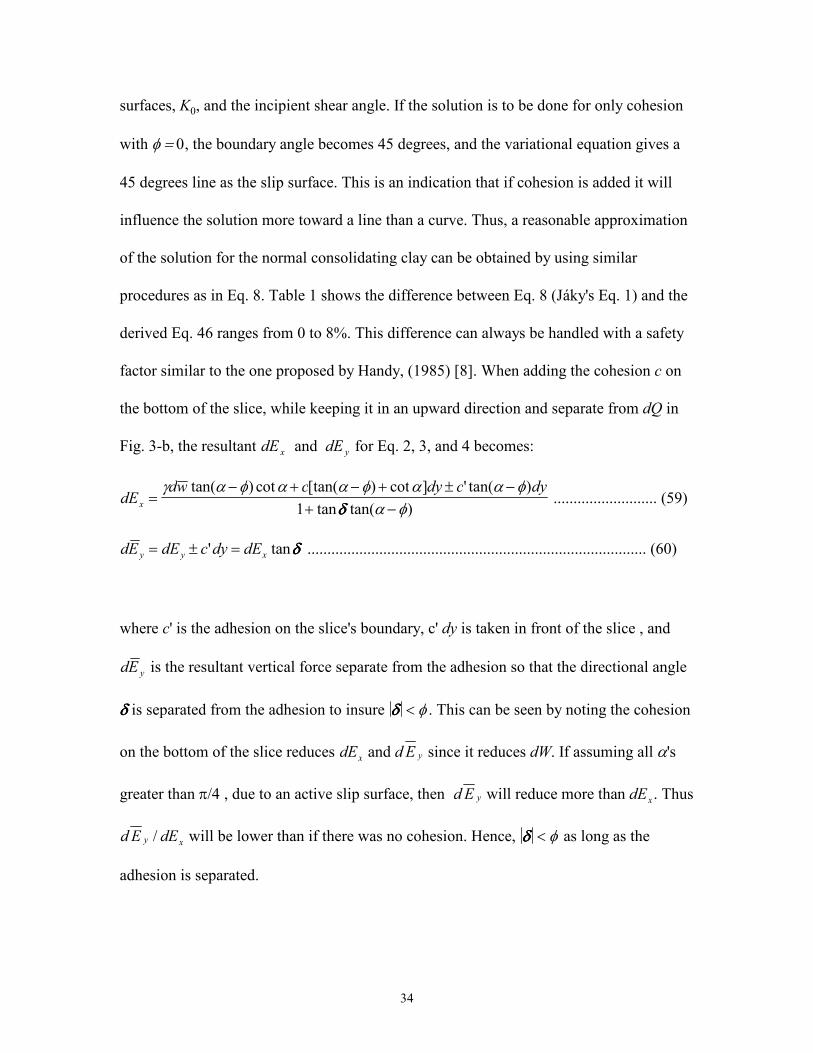
Fig. 3-b, the resultant dE dEx y and for Eq. 2, 3, and 4 becomes:

dEdw c dy c dy

x =− + − + ± −

+ −γ α φ α α φ α α φ

α φtan( ) cot [tan( ) cot ] ' tan( )

tan tan( )1 δδδδ .......................... (59)

dE dE c dy dEy y x= ± =' tanδδδδ ..................................................................................... (60)

where c' is the adhesion on the slice's boundary, c' dy is taken in front of the slice , and

dE y is the resultant vertical force separate from the adhesion so that the directional angle

δδδδ is separated from the adhesion to insure δδδδ < φ . This can be seen by noting the cohesion

on the bottom of the slice reduces dE dEx y and since it reduces dW. If assuming all α's

greater than π/4 , due to an active slip surface, then d E dEy x will reduce more than . Thus

d E dEy x/ will be lower than if there was no cohesion. Hence, δδδδ < φ as long as the

adhesion is separated.

35

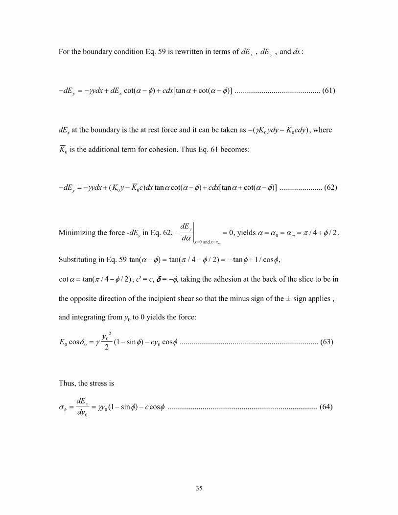
For the boundary condition Eq. 59 is rewritten in terms of dE dE dxx y , , and :

− = − + − + + −dE ydx dE cdxy xγ α φ α α φcot( ) [tan cot( )] ............................................ (61)

dEx at the boundary is the at rest force and it can be taken as − −( )γK ydy K cdy0 0 , where

K0 is the additional term for cohesion. Thus Eq. 61 becomes:

− = − + − − + + −dE ydx K y K c dx cdxy γ α α φ α α φ( ) tan cot( ) [tan cot( )]0 0 ...................... (62)

Minimizing the force -dEy in Eq. 62, − == =

dE

d

y

x x xmα

0

0 and

, yields α α α π φ= = = +0 4 2m / / .

Substituting in Eq. 59 tan( ) tan( / / ) tan / cosα φ π φ φ φ− = − = − +4 2 1 ,

cot tan( / / )α π φ= −4 2 , c' = c, δδδδ = −φ, taking the adhesion at the back of the slice to be in

the opposite direction of the incipient shear so that the minus sign of the ± sign applies ,

and integrating from y0 to 0 yields the force:

Ey

cy0 0

0

2

021cos ( sin ) cosδ γ φ φ= − − ....................................................................... (63)

Thus, the stress is

σ γ φ φh

xdE

dyy c= = − −

0

0 1( sin ) cos ............................................................................. (64)

36

The most remarkable conclusion in Eq. 64 is that K0 for clay is not constant when using

σ σ σ γh v h y/ /= . Preliminary investigation indicates that even if the closed form solution

is achieved the result is the same. But each term is still individualized by y0. In

consideration of the simplicity of Eq. 64, other notable remarks can be made: (1) The

equation is consistent with soil mechanics equations with cohesion such as active

pressure, passive pressure and bearing capacities, where the cohesion and the

cohesionless terms are two separate terms and not mixed. (2) The distance to zero stress

calculated in active condition is at y c Ka1 2= / γ , and Eq. 64 gives one half this

distance. This indicates that during a wall movement from at rest condition until an active

condition the surcharge due to the tension zone increases by 1/2. This is also consistent

with common sense, since one expects y1 to be between zero, or no tension, and the active

tension zone, the maximum tension zone. 1/2 is exactly the average value. (3) If

considering the undrain shear strength Su, the stress becomes σ γh uy S= − , which is

greater than the active condition γy Su− 2 . This is expected from the at rest condition to be

higher than the active condition for short-term loading. (4) When the ground is at rest,

and due to gravity weight, tension must exist on top causing tension cracks from

earthquake or any traction force. Comparing with elasticity, the elastic solution gives zero

stress on top, which is contrary to physical evidence. Tension cracks exist in clay even in

the at rest condition due to earthquake or any traction force. From these considerations,

Eq. 64 offers a reasonable working formula for normally consolidated clay.

37

Comparison with Experimental value for Clay

Unfortunately, all the available tests did not account for cohesion. If considering

Kc

y

h

v

0 1= = − −σσ

φγ

φsin cos , the test will match depending on the load applied with σh.

Thus, if σh is high , so the overburden is high, then c ycos /φ γ becomes a small number

and in this case K0 1≅ − sinφ matches Mayne and Kulhawy, (1982) [17]. On the other

hand, Brooker and Ireland, (1965) [2], recommended K0 0 95= −. sinφ for five different

kinds of clay. This may be an indication that c was high for these clays and the term

c ycos /φ γ reduces the overall K0. For example: if γy = 94psi, for a high overberden, c =

5psi and φ = 20o, it gives c ycos /φ γ = 0.05 for the clay used in their experiments. This

cohesion to initial stress ratio accounts for the overall reduction in K0. In any case, Eq. 64

suggests new verifications tests are necessary for clay. This becomes a primary

recommendation of this manuscript.

Overconsolidation in Clay

If setting the c = 0 in the closed form solution for clay (if obtained), the results must be

the same as the equations for cohesionless soil. Thus, the equation of overconsolidation

of sand, Eq. 54, must be modified for clay, where E n yh'≠ . Substituting and integrating

from y0 to 0 over all sets of slip surfaces for cohesionless terms, and integrating over y0

to y2 for the overconsolidating term, yields

38

( )dE Ky

Ee e

e ey yx L

e c

i c

L

D

∫ = +−−

−

−γ

γγ0

0

2

0 221' ........................................................... (65)

where y2 is the distance from the top of surface where overconsolidation stress starts.

Adding back the cohesion term to the equation, and expressing it as stress as in Eq. 64,

yields

σ γ φ φγγh L

e c

i c

L

D

y c Ee e

e e= − − +

−−

−

( sin ) cos '1 1 ......................................................... (66)

Note: the additive term in Eq. 66 for overconsolidation is independent of φ and y,

predicting a constant value throughout the ground, when higher than the cohesion term.

This constant value is very reasonable for clay when E ' is constant with depth. However,

in practice the additive term for overconsolidation should start at a distance at least

greater than y1 (the distance of tension in the ground). This is necessary since locked-in

stresses cannot occur on the top surface.

When repeating the analysis in a higher dimension, as in a circular or square plate with

plane strain analysis, equation 66 is replaced by:

σ γ φ φν ν

γγh L

e c

i c

L

D

y c Ee e

e e= − − +

−

− + −−

( sin ) cos '

( )( )1

1

1 1 21 ............................. (67)

Eq. 67 is preferred than Eq. 66 since it is more realistic.

39

If defining OCR = + = +( ) / /σ σ σ σ σ0 1 0 1 01 , where σ0 is the initial stress γLy, and

σ σ0 1+ is the initial plus the overburden stress, then the additive term can be expressed

as:

( )q ye e

e eK

e e

e e

e c

i c

e c

i c

h( ) =−

−=

−

−−0 1 1σ σOCR ................................................................ (68)

where σh is of Eq. 64. Substituting Eq. 68 in Eq. 66 to replace the additive term yields:

[ ] ( )σ γ φ φ γ φ φh L L

e c

i c

y c y ce e

e e= − − + − −

−

−

−( sin ) cos ( sin ) cos1 1 1OCR .................. (69)

and

( )Kc

y

e e

e ec

L

e c

i c

0 1 1 1= − −

⋅ +

−

−−

sin

cosφ

φγ

OCR ...................................................... (70)

Eq. 70 indicates K0c varies linearly with OCR for a constant expansion to compression

deflection ratio independent of OCR, and for a given initial stress γLy. If comparing Eq.

70 with Brooker and Ireland, (1965) [2] for five clays, four clays gives a secant slope of

0.075 (Chicago Clay, London Clay, Goose Lake Flour, and Weald Clay), and one clay

gives 0.042 (Bearpaw Shale). This gives an expansion to compression deflection ratios of

0.13, 0.11, 0.14, 0.12, and 0.06 respectively. This is a very reasonable expansion to

compression deflection ratio ( ) / ( )e e e ee c i c− − for clay. Thus, Eq. 70 appears to be a

reasonable approximation.

40

Conclusion

The mystery of why Jáky's equation agrees with experimental data is resolved.

Furthermore, the established incipient shear failure mechanism in obtaining K0 should

satisfy many engineers and scholars who believe K0 should not be related to failure

parameters (φ & c), since no failure criterion seem to appear in the at rest condition.

Additionally, the incipient shear failure mechanism offers solutions for other problems

besides K0. Variational method has been used in the analysis to obtain a closed form

solution for K0 for sand. The methods are classical and conventional and only practical

assumptions were used. The extremum condition indicates the existence of two slip

surfaces back to back. If using a line approximation with the same boundary condition the

result is identical to Jáky's equation. On the other hand if using the closed form equation,

the result is a slightly higher value for K0. The derived K0 is in excellent agreement with

experimental results and matches safety factor recommendations for Jáky's K0. The

corresponding slip surfaces are in excellent agreement with rigid reinforced earth walls.

The analysis was carried out further to establish physical criterion and equations for

overconsolidating sand. The result is in fair agreement with experiments and shows the

different parameters influencing the locked-in forces. Finally, the analysis is repeated for

deriving K0 for normal and overconsolidating clay. The slip surface used is approximate,

but gives a reasonable approximation for K0. The results are in good standing with

experiments. The derived equations were used to determine the tension zone distance in

clay. This distance is one half the active distance and is very reasonable. In general, in

clay, K0 is not constant with depth as apparent in the results. The paper offers the real K0

with a high confidence factor. However, further experiments and research are necessary

41

to verify the many consequences of using variational methods. The following are

recommended experiments and research:

1) Experiment to verify the tension zone distance in clay.

2) Experiment to verify the effect of c in K0 in clay.

3) Further research is needed in overconsolidating clay since the additive term related to

OCR is shown experimentally non-linear indicating the expansion to compression

deflection ratio is dependent on OCR.

The derivation can be readily extended for a slanted wall with a sloped soil on surface.

This in turn prepares the way for dynamic analysis. The theory can also be extended for

multi-layers of different soils in the ground. The equations derived in this manuscript are

expected to be used in a wide variety of engineering practice.

Acknowledgments

The writer is deeply appreciative to his wife Bernice J.F. Chouery and his mother Yvonne

E. Chouery for the love and patience in giving valuable family support to do this

manuscript. Also, he is thankful to the assistance provided by Shirley A. Egerdahl in

proofreading this manuscript. Many thanks to Prof. John F. Stanton, Prof. Colin B.

Brown, and Prof. Sunirmal Banerjee of the University of Washington for their support

during graduate study and in their continuous encouragement.

42

Appendix I.-References

1. Bishop, A. W. (1955). "The Use of Slip Circle in the Stability Analysis Analysis of

Slopes," Géotechnique, London, England, Vol. 5, No. 1, pp. 7-18.

2. Brooker, E. W., and Ireland, H. O., (1965). "Earth Pressures at Rest Related to Stress

History," Canadian Geotechnical Journal, National Research Council, Ottaws,

Ontario, Vol. II, No. 1, pp. 1-15.

3. Coulomb, Charles Augustin (1776). "Essai sur une application des règles de maximis

et minimis à quelques problèmes de statique relatifs à l'architecture," Mem. Div.

Savants, Acad. Sci., Paris, Vol. 7.

4. D'Appolonia, D. J., Lambe, T. W., and Poulos, H. G. (1971). "Evaluation of Pore

Pressures Beneath an Embankment," Journal of Soil Mech. and Foundations Div.,

ASCE, 97(SM6), pp. 881-867.

5. DeLory, F. A., and Salvas, R. J. (1969). "Some Observations on the Undrain Shearing

Strength Used to Analyze a Failure," Can. Geotech. J., 6(2), pp. 97-110.

6. Donaghe, R. T., and Townsend, F. C. (1978). "Effects of Anisotropic Versus Isotropic

Consolidation in Consolidated Undrained Triaxial Compression Tests of Cohesive

Soil," Geotech. Test. J., ASTM, 1(4), pp. 173-189

7. Fang, Y-S, and Ishibashi, I. (1986). "Static Earth Presures with Various Wall

Movements," J. of Goetech. Engrg., ASCE, 112(3), pp. 317-333

8. Handy, R. L. (1985). "The Arch in Soil Arching," J. Geotech. Engrg., ASCE, 111(3),

pp. 302-318.

43

9. Handy, R. L. (1983). Discussion of "K0 - OCR Relationships in Soil," by P. W. Mayne,

and F. H. Kulhawy, J. of Geotech. Engrg., ASCE, (109)6, pp. 862-864

10. Jáky, J. (1944). "A Nyugalmi Nyomás Tényezóje," Magyar Mérnok es Epitész Egylet

Kozlonye (Journal of the Society of Hungarian Architects and Engineers), pp. 355-358

11. Jáky, J. (1948). "Pressure in Silos," Proceedings of the Second International

Conference on Soil Mechanics and Foundation Engineering, Vol. I, pp. 103-107

12. Juran, I., Beech, J., and De Laure, E. (1984). "Experimental Study of the Behavior of

Nailed Soil Retaining Structures on Reduced Scale Models," Proc. Int. Symp. In-Situ

Soil and Rock Reinforcement, Paris, France.

13. Juran, I., and Christopher, B. (1989). "Laboratory Model Study on Geosynthetic

Reinforced Soil Retaining Walls," J. Geotech. Engrg., ASCE, 115(7), pp. 905-926.

14. Juran, I., Ider, H. M., and Farrag., K. (1990). "Strain Compatibility Analysis for

Geosynthetics Reinforced Soil Walls," J. Geotech. Engrg., ASCE, 116(2), pp. 312-

329.

15. Khera, R. P., and Krizek, R. J. (1967). "Strength Behavior of an Anisotropically

Consolidated Remolded Clay, " Highway Research Rec., 190, pp 8-18.

16. Koutsoftas, D. C., and Ladd, C. C. (1985). "Design Strength for an Offshore Clay," J.

Geotech. Engrg., ASCE, 111(GT3), pp. 337-355.

17. Mayne, P. W., and Kulhawy, F. H. (1982). K0 - OCR Relationships in Soil," J. of

Geotech. Engrg., ASCE, (108)6, pp. 851-872.

18. Mesri, G., and Castro M. A. (1987). "Cα/Cc Concept and K0 during Secondary

Compression," J. of Geotech. Engrg., ASCE, (113)3, pp. 230-247.

44

19. Nakase, A., and Kamei, T. (1983). "Undrained Shear Strength Anisotropy of Normally

Consolidated Cohesive Soils," Soils Found., 23(1), pp. 91-101.

20. Nakase, A., and Kobayashi, M. (1971). "Change in Undrained Shear Strength of

Saturated Clay Due to Rebound," Proceedings of the 4th Asian Regional Conference

on Soil Mechanics and Found. Engineering, Bangkok, Thailand, Vol. 1, pp. 147-150

21. Sherif, M. A., and Fang, Y. S. (1984). "Dynamic Earth Pressures on Walls Rotating

about the Top," Soil and Foundations, Japanese Society of Soil Mechanics and

Foundation Egineering, Vol. 24, No. 4, pp. 109-117.

22. Sherif, M. A., Fang, Y. S., and Sherif, R. I. (1984). "Ka and K0 Behind Rotating and

Non-Yeilding Walls," J. of Geotech. Engrg., ASCE, (110)1, pp. 41-56.

23. Sherif, M. A., Ishibashi, I., and Do Lee, Chong (1982). "Earth Pressures Against Rigid

Retaining Walls," J. of Geotech. Engrg., ASCE, (108)5, pp. 679-695.

24. Terzaghi, K. (1955). "Evaluation of Coefficients of Subgrade Reaction,"

Geotechnique, Vol. 5.

25. Terzaghi, K. (1941). "General Wedge Theory of Earth Pressures," Trans. Am. Soc.

Civil Eng. No.106, Vol. 67, pp. 68-80

26. Terzaghi, K. (1934). "Large Retaining-Wall Tests," Engineering News-Record, Vol.

112, pp. 136-140, 259-262, 316-318, 403-406, 503-508.

27. Timoshenko, S. P., and Goodier, J. N. (1970). Theory of Elasticity, McGraw-Hill

Book Company Inc., New York, N. Y., 3rd Edition, p. 97.

28. Tschebotarioff, G. P., (1953). Soil Mechanics Foundations and Earth Structures,

McGraw-Hill Book Company Inc., New York, N. Y., p. 256.

45

29. Weinstock R., (1974), Calculus of Variations With Applications to Physics and

Engineering, Dover Publications, Inc., New York, N. Y., pp. 22-25, and pp. 36-40.

Appendix II.- Notation

The following symbols are used in this paper:

α = angle of the failure wedge, or of failure a slice, with the horizontal;

α0 = slice wedge angle with the horizontal at start of first slip surface at x = 0;

αm = slice wedge angle with the horizontal at end of second slip surface;

αn = slice wedge angle at end of first slip surface or start of second slip surface;

c = cohesion in clay;

c' = adhesion on the slice boundary;

D = x - term used in experimental paper by others;

∆ = axial deflection of a beam;

δδδδ = Coulomb friction, directional frictional angle between dEx and dEy;

δ0 = directional angle at first slice boundary at x = 0 = incipient shear angle;

δi = directional angle at slice boundary at x;

δm = directional angle at last slice boundary at x = xm = incipient shear angle;

δn = directional angle at slice boundary at x = xn;

E = elastic modulus of beam;

E ' = spring modulus of soil;

E0 = directional force of first slice boundary at x = x0;

46

Eh = horizontal force at rest;

∆Eh = change in horizontal force;

Ei = directional force of slice boundary at x;

Em = directional force of last slice boundary at x = xm;

En = directional force of slice boundary at x = xn;

dEx = slice horizontal resultant force;

dEy = slice vertical resultant force;

dE y

= resultant of vertical force on a slice separate from slice adhesion;

ec = compressed void ratio at full load;

ee = expansion void ratio at rebound or at load removal;

ei = initial voids ratio at loose state;

F = immobile friction force;

∆F = change in immobile friction force;

φ = angle of internal friction of soil;

γ = soil unit weight;

γD = unit weight of soil at dense state or at rebound state;

γL = unit weight of soil at loose state or initial state;

H = y - term used in experimental paper by others;

h = mathematical coefficient in the slip surface equations;

h' = mathematical coefficient in the slip surface equations related to h;

i = integer counter;

Κ = coefficient of lateral earth pressure or lateral stress ratio;

47

K0 = at rest earth pressure coefficient;

K0 = additive term for the coefficient of earth pressure for cohesion;

K0c = coefficient of lateral earth pressure at rest for overconsolidation;

K1 = dimensionless coefficient representing a term in an equation;

Ka = active earth pressure coefficient;

Kp = passive earth pressure coefficient;

kh = ( / )[( ) / ( )]n e e e eh D e c i cγ − − ;

L = length of beam;

m = integer;

Mx = total moment of the horizontal forces of all the slices;

My = total moment of the vertical forces of all the slices;

ν = Poisson's ratio;

N = normal force;

∆N = change in normal force;

n = integer;

nh = subgrade modulus of sand;

OCR = overconsolidation ratio;

P = locked-in force in a beam;

P1 = downward shear force on wall;

P2 = upward shear force on wall;

dQ = reactive force on bottom of failure wedge or slice to maintain equilibrium;

q = uniform surcharge pressure;

48

q(y) = unknown horizontal stress for overconsolidation;

q0(y) = uniform surcharge load that causes locked-in force in a beam;

qc(y) = prehistoric surcharge;

ℜ = calculus of variation function of mixed variables representing the integrand;

r = correlation number;

S/H = x/y0 - term used in experimental paper by others;

Su = undrain shear strength for short term loading;

σ0 = initial stress = γLy - in overconsolidations;

σ1 = overburden stress in overconsolidations;

σh = the horizontal stress in soil;

σv = the vertical stress in soil;

T = incipient shear;

W = vertical force from weight of wedge;

dW = weight of slice;

dw = weight of slice times tanα;

Ω = dimensionless variable = x/y0;

x = coordinate x-axis;

dx = width of slice's wedge;

′x = dx/dy;

xm = distance to tip of second slip surface;

ψ = dimensionless variable = y/y0;

y = coordinate height at y-axis;

49

dy = height of slice's wedge;

′y = dy/dx;

y0 = height of wall or start of first slip surface at x = 0;

y1 = tension zone distance in clay;

y2 = distance from the top surface to where the overconsolidation stress starts;

ym = height distance at end of second slip surface;

yn = height distance at end of first slip surface or start of second slip surface;

Z/H = y/y0 - term used in experimental paper by others;

dz = beam thickness;

Appendix III.- Numerical Check

With the advent of software technology, numerical differentiation and integration

easily has become easier. Algebra can be checked from one equation to a reduced

equation by numerical substitution to give identical values. Many software programs are

available to do the checking. All of the derived equations were checked with MATHCAD

on a personal computer, including starting with the variational (Euler equation). The

following constants' relations are necessary if the reader needs to double-check the

writer:

Eq. 22 .................................................................... hh

'sin cos

= −2γ φ φ

;

50

and

Eq. 34 .................................................................... hh

'sin

=2 2γ φ

.

Note: when using Sherif's expression their recommendations were to use γD and K0 =

1 - sinφ for calculating the forces and the stresses. This effects the comparison slightly.

Analysis shows the average kh = 5.87 instead 5.5 in the region 32 < φ < 44 degrees and

1.03 < γD/γL < 1.07. The analysis used K0 from Eq. 46 and used γL in calculating the

forces and the stresses.