86

Excel Program :

- It is one of the most commonly used electronic Table program.

- Excel file is a ( Workbook ) consisting of ( Worksheets ) and each

sheet consists of ( Columns ) and ( Rows ) and their intersection

results in ( Cells ) .

Uses of Excel program ;

1- The works that need arithmetic operations.

2- Repeating the arithmetic operations easily and the auto correction of

the result when changing the values.

3- Representing data in the form of charts with different formations.

Starting Excel program :

Start ………. All Program -------- Microsoft Excel

Components of the Startup Screen of Excel program :

1- Title Bar : Displays the default title of the workbook which is

( Book1 ) in addition to the program title and icon.

2- Menu Bar : Contains a set of menus containing options.

3- Standard Bar : Contains a set of icons as shortcuts of important

commands in the menus.

4- Formatting Bar : Contains a set of icons as shortcuts of the

formation options.

5- Formula Bar : Is used for typing equations and it displays the cell

value whether it is ( text – numbers – functions ).

6- Horizontal and Vertical Scroll Bars : To view the hidden parts of

the worksheet.

When starting the program we will find that the workbook is

consisting from 3 sheets ( Sheet1 – Sheet 2 – Sheet3 ) and each sheet

displays a set of columns that are ordered by the English alphabets ,

and rows taking serial numbers.

87

( The number of columns is 256 – The number of rows in the sheet is

65536 )

Workbook : It indicates to the Excel file which contains a set of

worksheets.

Work Book : Is used in entering data to be saved in files.

Worksheet : Consists of a set of columns and rows .

Cells : They are the result of the columns and rows intersection and

each cell has a title that is determined according to the column and

row ( A3 , B4 ).

Active Cell : It is a selected cell that a black border appears around

it .

Browsing the workbook ( Moving from a worksheet to

another )

First : By using Mouse

1- Click on the sheet title ( Sheet 1 – Sheet2 – Sheet 3 ) from the

Navigation bar.

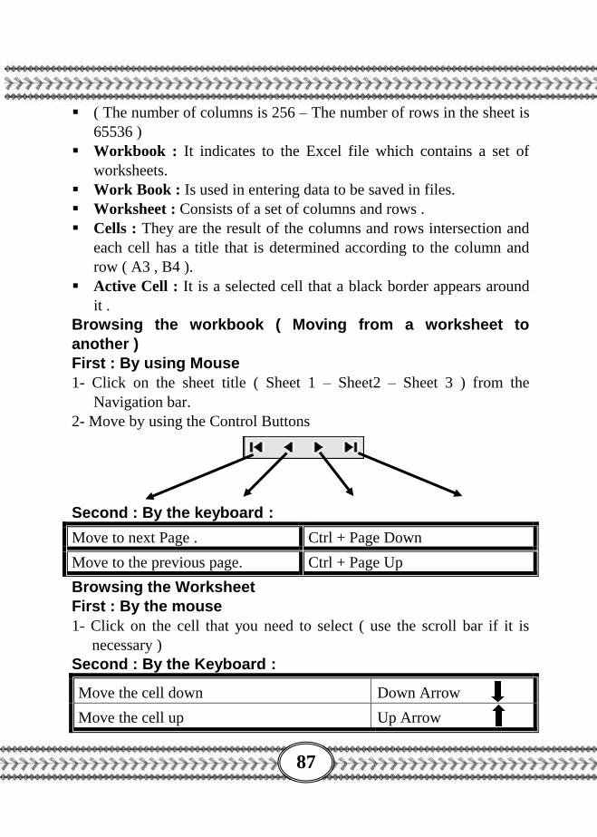
2- Move by using the Control Buttons

Second : By the keyboard :

Move to next Page . Ctrl + Page Down

Move to the previous page. Ctrl + Page Up

Browsing the Worksheet

First : By the mouse

1- Click on the cell that you need to select ( use the scroll bar if it is

necessary )

Second : By the Keyboard :

Move the cell down Down Arrow

Move the cell up Up Arrow

88

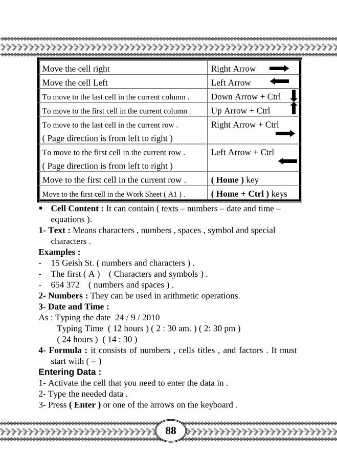
Move the cell right Right Arrow

Move the cell Left Left Arrow

To move to the last cell in the current column . Down Arrow + Ctrl

To move to the first cell in the current column . Up Arrow + Ctrl

To move to the last cell in the current row .

( Page direction is from left to right )

Right Arrow + Ctrl

To move to the first cell in the current row .

( Page direction is from left to right )

Left Arrow + Ctrl

Move to the first cell in the current row . ( Home ) key

Move to the first cell in the Work Sheet ( A1 ) . ( Home + Ctrl ) keys

Cell Content : It can contain ( texts – numbers – date and time –

equations ).

1- Text : Means characters , numbers , spaces , symbol and special

characters .

Examples :

- 15 Geish St. ( numbers and characters ) .

- The first ( A ) ( Characters and symbols ) .

- 654 372 ( numbers and spaces ) .

2- Numbers : They can be used in arithmetic operations.

3- Date and Time :

As : Typing the date 24 / 9 / 2010

Typing Time ( 12 hours ) ( 2 : 30 am. ) ( 2: 30 pm )

( 24 hours ) ( 14 : 30 )

4- Formula : it consists of numbers , cells titles , and factors . It must

start with ( = )

Entering Data :

1- Activate the cell that you need to enter the data in .

2- Type the needed data .

3- Press ( Enter ) or one of the arrows on the keyboard .

89

Modifying the cell content : ( Through the cell – or Formula bar )

Double click on the cell that you need to modify its content and

Select it and press ( F2 ) button on the keyboard .

We will note that the cursor will appear in the cell . correct the

mistakes .

Press ( Enter ) button to accept modifying the cell.

Saving Workbook :

1- Select Save or Save As from File menu.

2- Select a location from Save In.

3- Type the needed title and it is preferred to indicate to the content in

File Name .

4- Click Save and then we will note that the new name will appear in

File Name .

Close Work Book file :

It can be done by one of the following :

1- Open ( File ) menu and select ( Close ) .

2- Click (Close) icon in the right corner in the program internal

window .

Close Excel program :

It can be done by one of the following ways :

1- Open ( File ) menu and select ( Exit ).

2- Click on Close icon in the right corner in the program window .

Using ( Work Sheet – Rows – Columns – Cells )

The Selection :

- It is to select a certain part of the Work Sheet to apply an effect to

it .The selection is of the important ways for using some options in

Excel program .

90

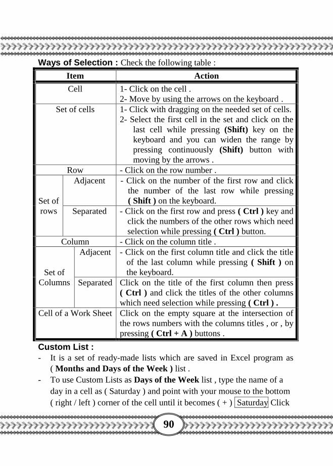
Ways of Selection : Check the following table :

Item Action

Cell 1- Click on the cell .

2- Move by using the arrows on the keyboard .

Set of cells 1- Click with dragging on the needed set of cells.

2- Select the first cell in the set and click on the

last cell while pressing (Shift) key on the

keyboard and you can widen the range by

pressing continuously (Shift) button with

moving by the arrows .

Row - Click on the row number .

Set of

rows

Adjacent - Click on the number of the first row and click

the number of the last row while pressing

( Shift ) on the keyboard.

Separated - Click on the first row and press ( Ctrl ) key and

click the numbers of the other rows which need

selection while pressing ( Ctrl ) button.

Column - Click on the column title .

Set of

Columns

Adjacent - Click on the first column title and click the title

of the last column while pressing ( Shift ) on

the keyboard.

Separated Click on the title of the first column then press

( Ctrl ) and click the titles of the other columns

which need selection while pressing ( Ctrl ) .

Cell of a Work Sheet Click on the empty square at the intersection of

the rows numbers with the columns titles , or , by

pressing ( Ctrl + A ) buttons .

Custom List :

- It is a set of ready-made lists which are saved in Excel program as

( Months and Days of the Week ) list .

- To use Custom Lists as Days of the Week list , type the name of a

day in a cell as ( Saturday ) and point with your mouse to the bottom

( right / left ) corner of the cell until it becomes ( + ) Saturday Click

91

on the other cells with dragging the other cells to complete the

remaining days of the week . That is called ( Filling a series of

data ) .

Insert ( Cells – Rows – Columns – Work Sheet ) First : Insert ( Cells ) : - You can insert cells to a certain location in the Work Sheet by

using one of the following ways :

1- Open ( Insert ) menu and select ( Cells … ) .

2- Right click on the cells and select ( Insert ) from the shortcut menu .

The following window will appear : It will help to :

1- Insert cells in the selected location and move the cells to the right.

2- Insert cells in the selected location and move the cells down.

3- Insert cells in new rows.

4- Insert cells in new columns .

- To insert a certain number of cells per time , you should first select the

cells according to the needed number of cell.

Second: inserting Rows : 1- Select a row or a set of rows.

2- Open ( Insert ) menu and select ( Rows ) or open the shortcut menu

and select ( Insert ).

3- Rows will be inserted above the selected rows and with the same

number of rows .

Third : Inserting Columns : 1- Select a column or a set of columns.

2- Open ( Insert ) menu and select ( Columns ) or open the shortcut

menu and select ( Insert ).

Forth : Inserting Worksheet : 1- Select the sheet that you need to insert one before it.

2- Open ( Insert ) menu and select ( Worksheet ) .

3- A new sheet will be inserted before the selected sheet.

- You can insert a worksheet through the shortcut menu of the

worksheet and select ( Insert ) , a window will appear select

( Worksheet ).

92

Delete ( Cells – Rows – Columns – Worksheet )

First : Delete Cells :

1- Select a cell or a set of cells which you need to delete.

2- Open ( Edit ) menu and select ( Delete ) .

- Or, right click on the cell and select ( Delete … ) .

3- The following window will appear. It helps in the following :

a. Delete the selected cells and move the adjacent cells to the left side .

b. Delete the selected cells and move the adjacent cells up .

c. Delete the selected cells and rows which contain the cells.

d. Delete the selected cells and columns which contain the cells.

Second : Delete Rows : 1- Select the row or set of rows that you need to delete .

2- Open ( File ) menu and select ( Delete ) .

Or , open the shortcut menu and select ( Delete ).

3- The selected row or rows will be deleted .

Third : Delete Columns : 1- Select the columns or set of columns that you need to delete .

2- Open ( Edit ) menu and select ( Delete ).

Or , open the shortcut menu and select ( Delete ).

3- The selected column /columns will be deleted .

Forth : Delete Worksheet : 1- Select the Worksheet that you need to delete .

2- Open ( Edit ) menu and select ( Delete Sheet ) .

Or , open the shortcut menu and select Delete .

3- The selected worksheet will be deleted .

- When inserting or deleting cells , rows or columns , the number of

the columns and rows in the page will remain without change.

Format :

- It means to set the item form and properties as ( Worksheet –

Column – Row – Cells ) .

Ways of Formation : 1- From ( Format ) menu . 2- From the shortcut menu .

3- From Format Tool Bar .

93

First : Worksheet Format : Open ( Format ) menu.

Select ( Sheet ) .

Rename : To change the current Worksheet name.

Hide : To hide the current Worksheet.

Unhide : To show the hidden Worksheets .

Background : To insert a background to the worksheet.

Second : Format Columns : Select the needed column / columns.

Open ( Format ) menu.

Width : To change the width of the selected column / columns or

select Column Width from the shortcut menu.

AutoFit selection : An automatic setting of the column width

( according to its content ) .

Hide : To hide the selected column / columns.

Unhide : To show the hidden column / columns .

Standard Width : To change the standard width of all the columns

in the worksheet.

Third : Format Rows : Select the row / rows that need formation .

Open ( Format ) menu .

Height : To change the row height ( or Row Height from the

shortcut menu ) .

AutoFit : To auto set the row height ( according to its content).

Hide : To hide the selected row / rows .

Unhide : To show the hidden row / rows .

Fourth : Cells Format : Select the cells that need formation .

Open ( Format ) menu.

Select ( Cells… ) .

Or , from the shortcut menu select ( Format Cells ) .

A window will appear containing a set of tabs .

1- ( Number ) tab : This tab is used to set the form and format of the

different uses of numbers as : date and time and currency .

94

2- ( Alignment ) tab : It is used to set the text alignment in the cells ,

sets the text orientation and merge cells.

3- (Font) Tab : It is used to set the font size , type and color in the cells .

4- ( Border ) Tab : To set internal and external borders to the cell .

5- ( patterns ) Tab : To set a background and pattern to the cells and to

change the pattern color.

Formula :

- The Formula makes the Excel program very useful .

- Formula helps to calculate the results of the data saved in the

Worksheet.

- The formula can be entered in the cell , so it can be copied , cut or

deleted .

- The formula starts with ( = ) followed by numbers and operations.

Uses of Formula :

1- The result of formula changes automatically when changing any value

in the formula.

2- The formula helps to modify or add information to the Worksheet .

Steps of Entering the Formula :

1- Select the cell where you need to insert the formula.

2- Type ( = ) .

3- Insert the first number or the title of the cell containing the first

number – or click the cell so the program with type its title.

4- Insert the Factor as ( / , * , - , + ) .

5- Insert the second number or the title of the cell containing the first

number – or click on this cell .

6- Then , press ( Enter ) key on the keyboard or click ( √ ) in the

Formula Bar to perform the arithmetic operation and insert the data

in the cell.

7- To cancel the formula or cancel inserting the data in the cell, click

( × ) in the Formula bar or press ( Esc ) on the keyboard.

- After applying the formula , the formula value appears in the cell

and the formula content appears in the Formula bar.

95

Formula Modification :

- The formula can be modified through the cell or Formula bar and

when applying the modification , the formula’s result will change

automatically .

Using the cells titles in the formula ( Cell Reference ) :

- It is preferred to use the cells titles in the formula ( = C2 + D2 ) that

this has several uses as in the following :

1- Changing the value of any used cell doesn’t need to change the

formula itself.

2- Using the ( Automatic Calculator ) , that Excel program takes the

new value in the cell and re-calculate automatically the formula and

then changes the result of the formula.

Using more factors in the Formula :

1- Percentage( % ) :

As : = A1 / A2 %

- To find the percent of the first cell ( A1 ) to the value of the second cell

( A 2 ) As : = 2 / 4 %

- The result will be (50) that (2) represents half of the number (4) .

2- The Power Sign ( ^ ) : - This factor is used to raise a number (basis) into another (power)

As : = D4^2 that means to raise the cell (D4) value to the power (2) .

Priorities of performing the Arithmetic Operations : 1- Solve what is between the brackets. 2- The Power Operation ( ^ ) .

3- Multiplication or Division , whatever is the first ( / * ) .

4- Addition or Subtraction , whatever is the first ( + - ) .

- The formula is solved from left to right.

Example :

- The solution of the formula = 3 + 2 * 4 is ( 11 )

- The solution of the formula = ( 3 + 2 ) * 4 is ( 20 )

Functions : - Functions are based on the concept of formula to perform the work

easily and quickly . They are a ready-made formula which is used to

perform simple or complicated operations .

96

- As the most commonly used functions ( Sum , Average , Max ,

Min , Count A ) .

1- Sum Function :

- It is used to calculate the of a set of cells .

Example :

= Sum ( A3 , A4 , A5 , A6 )

= Sum ( A3 : A 6 )

- Then , press ( Enter ) key on the keyboard or click ( √ ) on the

Formula Bar to show the result.

2- Average Function :

Example :

It is used to get the average of a set of cells .

= Average ( A 3 , A4 , A5 , A6 )

= Average ( A3 : A6 )

3- Max function :

- It is used to find the maximum value among a set of values .

Example :

= Max ( A 3 , A4 , A5 , A6 )

= Max ( A3 : A 6 )

4- Min Function :

- It is used for calculating the minimum value among a set of values .

Example :

= Min ( A 3 , A4 , A5 , A6 )

= Min ( A 3 : A 6 )

5- CountA Function :

- It is used for counting the number of cells which have values only .

Example :

= CountA ( A 3 : A 6 )

Copying the formula :

- The formula can be copied from a cell to another by using one of the

following ways :

97

1- Using the options ( Copy and Paste ) from Standard

Toolbar or from ( Edit ) menu or Shortcut menu .

2- Using ( Auto Fill )

- Click when the pointer takes this shape and drag to the cells to

apply the same formula to them .

The Chart :

- It is a representation of data in the Worksheet to give a visual

analysis of information .

Types of Charts : 1- 2 D ( Two – dimensional ) .

2- 3 D ( Three – dimensional ) .

- The chart can be created in the same page which contain the table of

data and it may be in a separate page .

- The chart is related to the data in the Worksheet that , when

modifying the data , the chart will be automatically modified

Ways of creating the Chart :

1- select the cells that need to be represented.

2- Open ( Insert ) menu and Select the ( Chart ) .

3- Select Chart Wizard from Standard Toolbar.

Steps for creating the chart :

- After selecting to create the chart in any of the preceding ways, you

will pass through four stages before the creation steps :

1- Chart Type : To set the type of the chart ( 3D – 2 D )and click

( Next ) .

2- Chart Source Data : To set a chart source for the data that we need

to represent and click ( Next ) .

3- Chart Option : To set the chart options as : title , axis title of ( x , y )

and click Next

4- Chart Location : To set the chart location in the Workbook .

(1) As new Sheet : To set the chart in a new separate sheet.

(2) As object In : To set the chart in the form of an object in the same

sheet containing data .- Finally , click ( Finish ) .

98

Chart Modification :

- The chart can be modified through several ways as in the

following :

1- ( Chart ) Toolbar which appears when selecting the chart.

- When the ( Chart ) Toolbar doesn’t appear , open ( View ) menu

then select ( Toolbars ) and ( Chart ) .

2- The modification will be in any of the four steps through (Chart)

menu which appears in the menu bar when selecting (Chart) menu.

- To delete a chart , select it and press Delete button on the

keyboard .

Printing in Excel Program :

Page Setup :

- From ( File ) menu select ( Page Setup ).

- Then, ( Page Setup ) window appears containing a set of tabs as the

following :

First : Page tab

- It is used to set the page orientation ( Landscape ) or ( Portrait ).

- It is used to set the size of the page .

Second : Margins tab

- It helps to set the page margins ( margin is the empty space on the

sides and at the top and bottom of the page ) .

1- the ( Top ) margin. 2- the ( Bottom ) margin.

3- the ( Right ) margin . 4- ( Left ) margin .

5- the ( Header ) and ( Footer ) .

6- Alignment of the page contents Horizontally and Vertically .

Third : Header / Footer tab :

- It allows to insert a header and footer to the page when printing it .

- It is possible to insert previously prepared contents by the program to

the page header and footer by opening the menu down the words

( Header or Footer ) as :

(Page Number – Number of Pages - Date and Time – File Name … )

a- Custom Header b- Custom Footer .

99

Print Preview :

- You can make a print preview to check the page form and content

before printing.

- Ways of Preview :

1- Open ( File ) menu and select ( Print Preview ).

2- Click on ( Print Preview ) icon on Standard Toolbar .

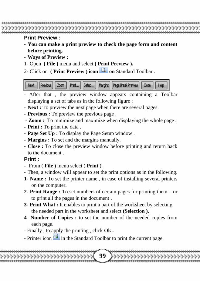
- After that , the preview window appears containing a Toolbar

displaying a set of tabs as in the following figure :

- Next : To preview the next page when there are several pages.

- Previous : To preview the previous page .

- Zoom : To minimize and maximize when displaying the whole page .

- Print : To print the data .

- Page Set Up : To display the Page Setup window .

- Margins : To set and the margins manually.

- Close : To close the preview window before printing and return back

to the document .

Print :

- From ( File ) menu select ( Print ).

- Then, a window will appear to set the print options as in the following.

1- Name : To set the printer name , in case of installing several printers

on the computer.

2- Print Range : To set numbers of certain pages for printing them – or

to print all the pages in the document .

3- Print What : It enables to print a part of the worksheet by selecting

the needed part in the worksheet and select (Selection ).

4- Number of Copies : to set the number of the needed copies from

each page.

- Finally , to apply the printing , click Ok .

- Printer icon in the Standard Toolbar to print the current page.