統計學 : 應用與進階第 6 章 : 常用的連續隨機變

數

均勻隨機變數 指數隨機變數 指數隨機變數與 Poisson 隨機變數之間的關係 常態隨機變數

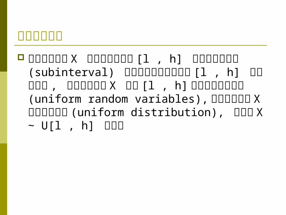
均勻隨機變數 如果隨機變數 X 的實現值在區間 [l , h] 中的任

何次區間 (subinterval) 的機率值為該次區間佔[l , h] 區間之比率 , 則稱隨機變數 X 為在 [l , h] 間的均勻隨機變數 (uniform random variables), 或稱隨機變數 X 服從均勻分配(uniform distribution), 我們以 X ∼ U[l , h] 表示之

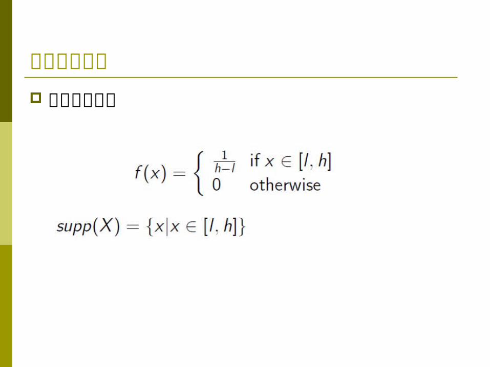
均勻隨機變數 機率密度函數

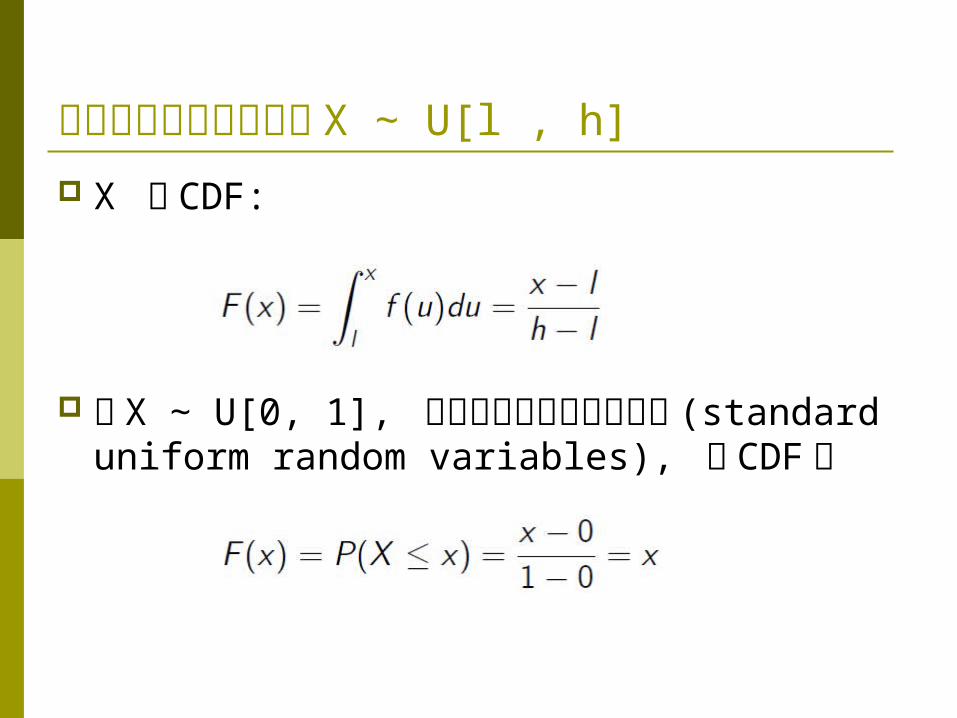
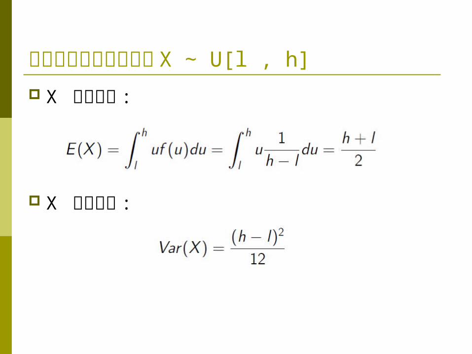
均勻隨機變數重要性質 X ∼ U[l , h]

X 的 CDF:

若 X ∼ U[0, 1], 稱之為標準均勻隨機變數(standard uniform random variables), 其CDF 為

均勻隨機變數重要性質 X ∼ U[l , h]

X 的期望值 :

X 的變異數 :

均勻隨機變數重要性質 X ∼ U[l , h]

X 的中位數 : x0.5 = E(X)

因此 , 我們可以解出

亦即均勻隨機變數的中位數等於期望值

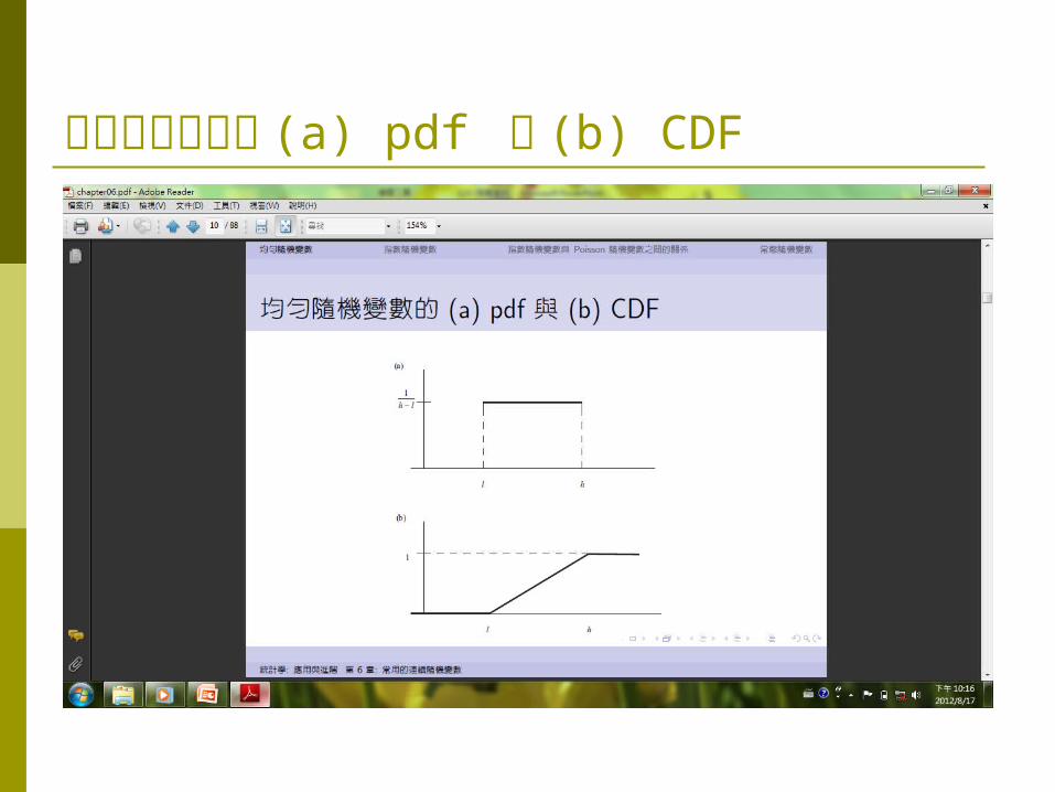
均勻隨機變數的 (a) pdf 與 (b) CDF

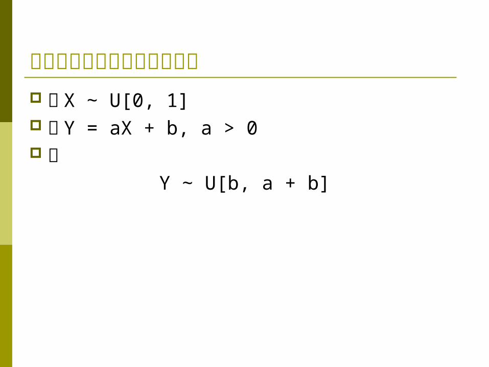
均勻隨機變數線性變換不變性 若 X ∼ U[0, 1] 且 Y = aX + b, a > 0 則

Y ∼ U[b, a + b]

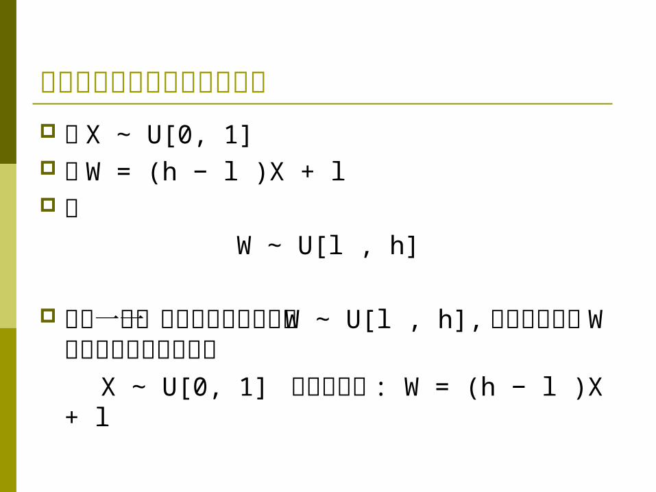
均勻隨機變數線性變換不變性 若 X ∼ U[0, 1] 且 W = (h − l )X + l 則

W ∼ U[l , h]

任何一個一般化的均勻隨機變數 W ∼ U[l , h],我們都可以將 W 寫成標準均勻隨機變數

X ∼ U[0, 1] 的線性函數 : W = (h − l )X + l

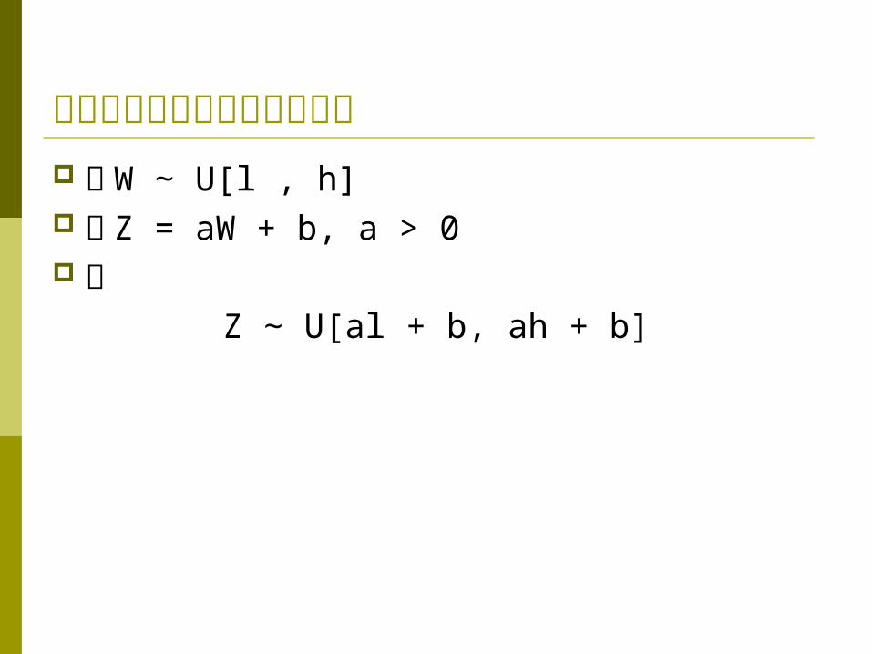
均勻隨機變數線性變換不變性 若 W ∼ U[l , h] 且 Z = aW + b, a > 0 則

Z ∼ U[al + b, ah + b]

均勻隨機變數的應用 網購賣家的底價為 $10,000 競標對手的出價為 X, 簡單假設 X ∼ U[10000,

15000] 試問① 如果你出價 $12,000, 試問你網購成功的機率 ?② 如果你出價 $14,000, 試問你網購成功的機率 ?③ 如果你想要極大化你的網購成功機率 , 請問你該 出價多少 ?

指數隨機變數 在間斷隨機分配中 , 我們介紹過 Poisson 分配 ,

衡量的是一段期間內 , 事件發生次數的機率 , 譬如說 , 一小時內出現的公車班次

相對應的 , 我們也可以衡量兩班公車之間的等待時間 , 而刻劃等待時間的機率分配即為指數分配

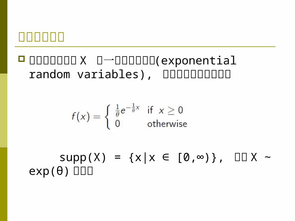
指數隨機變數 我們稱隨機變數 X 為一指數隨機變數

(exponential random variables), 如果其機率密度函數為

supp(X) = {x|x ∈ [0,∞)}, 並以 X ∼ exp(θ)

表示之

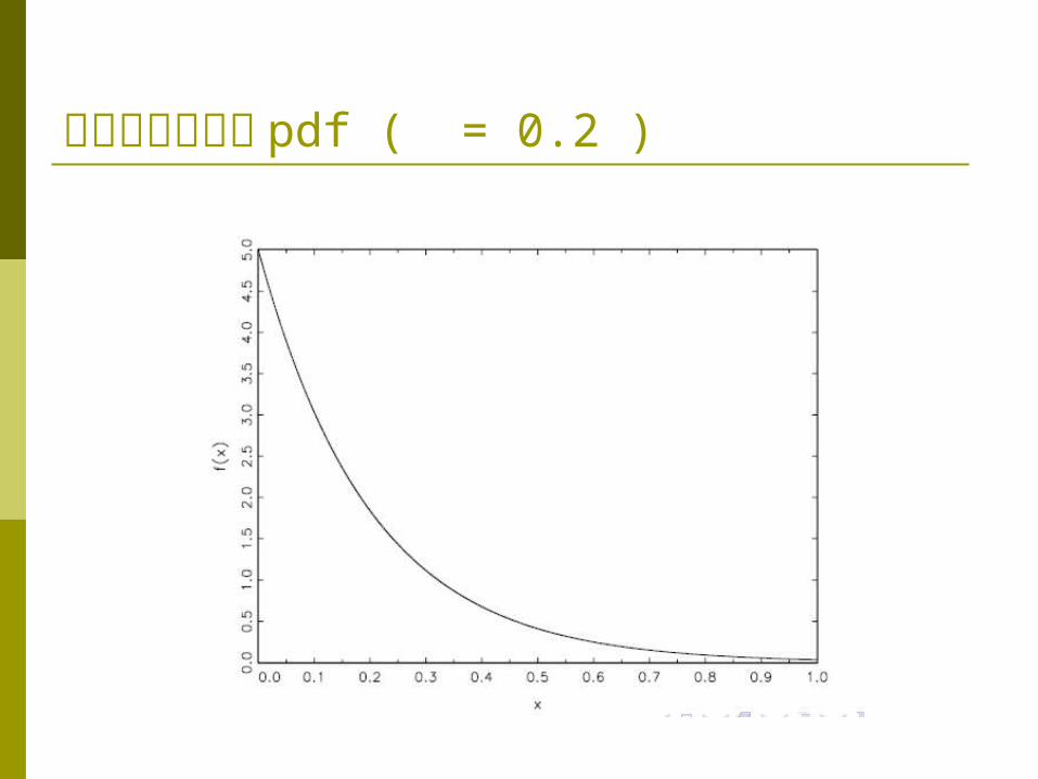
指數隨機變數的 pdf ( = 0.2 )

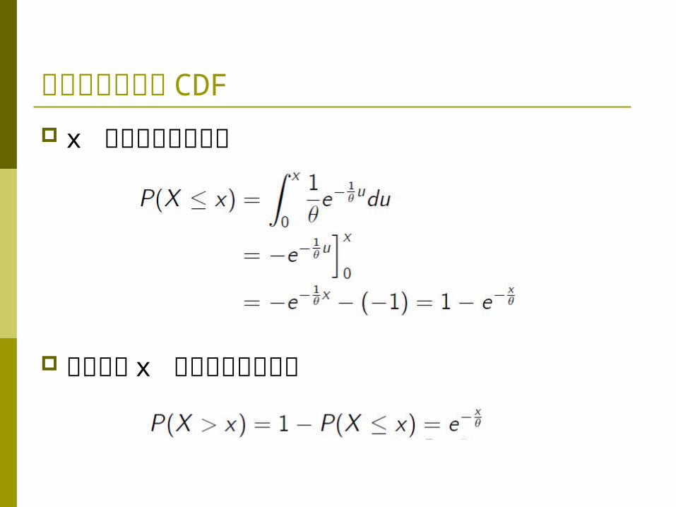
指數隨機變數的 CDF

x 分鐘內公車會到達

至少要等 x 分鐘公車才會到達

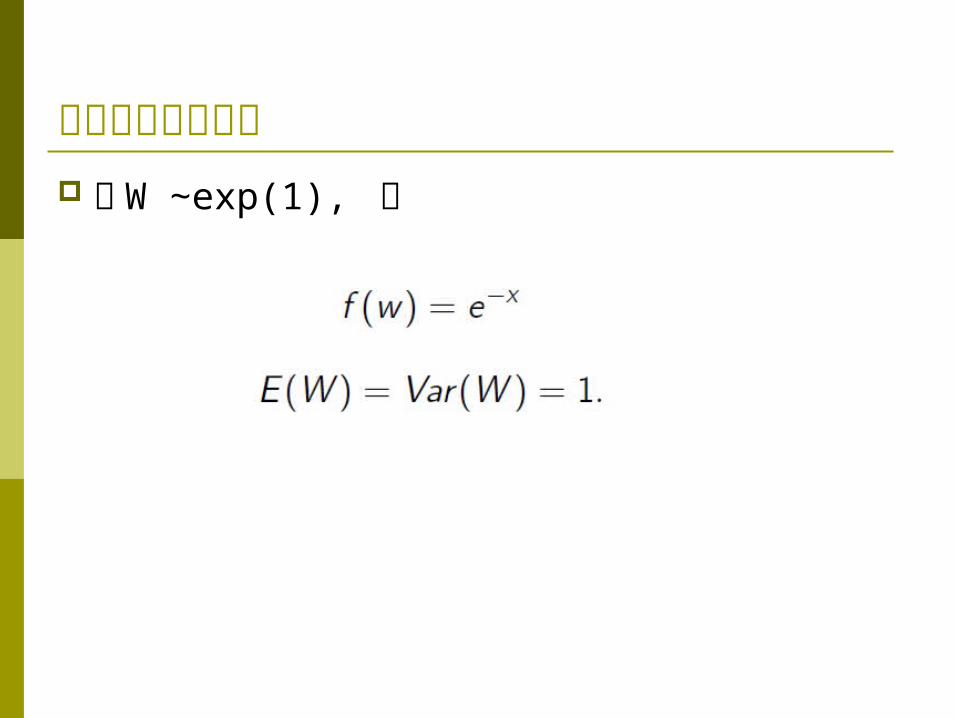
標準指數隨機變數 若 W ∼exp(1), 則

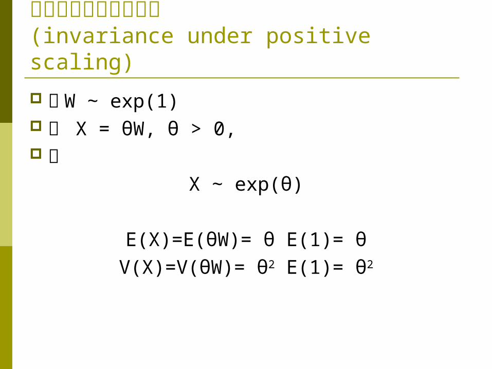
指數隨機變數的不變性(invariance under positive scaling)

若 W ∼ exp(1) 且 X = θW, θ > 0, 則

X ∼ exp(θ)

E(X)=E(θW)= θ E(1)= θV(X)=V(θW)= θ2 E(1)= θ2

θ 的意義 指數隨機變數除了用來刻劃「等待時間」 , 也可

用來刻劃「存續時間」 (length of life or duration)

因此 , 參數 θ = E(X) 除了可以詮釋為預期等待時間 , 也可以看做是預期存續時間 , 或稱預期壽命

指數隨機變數的無憶性 若 X ∼ exp(θ), P(X > m + n|X > m) = P(X > n) 譬如說 , 你已經在站牌底下等了 m 分鐘的公車 ,

此時 , 阿慶也加入等公車的行列。顯而易見的 ,無論是你或阿慶 , 至少再等 n 分鐘後公車才來的機率是相同的

也就是說 , 給定你已經等了 m 分鐘 , 然後你得至少再等 n 分鐘的條件機率 P(X > m + n|X > m) 等同於阿慶至少再等 n 分鐘的非條件機率P(X > n)

指數隨機變數 vs. Poisson 隨機變數 指數分配與 Poisson 分配猶如一體的兩面 , Poisson 分配 , 衡量的是一段期間內 , 事件發

生次數的機率 , 而指數分配衡量的是兩接連事件發生之間的等待時間

令 T 代表從零時 ( 原點 ) 開始直到第一次事件發生的等待時間。舉例來說 , T 代表今天第一班公車到來前的等待時間

指數隨機變數 vs. Poisson 隨機變數 等待時間 T 的機率分配為 : F(t) = P(T ≤ t) = 1 − P(T > t) = 1 − P( 在 [0, t] 的區間內沒有公車抵達 )

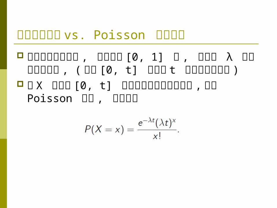
指數隨機變數 vs. Poisson 隨機變數 假設根據過去經驗 , 單位時間 [0, 1] 內 , 平均

有 λ 輛的公車會抵達 , ( 亦即 [0, t] 期間有 t 輛的公車會抵達 )

令 X 代表在 [0, t] 的區間內公車的抵達班次 , 根據 Poisson 分配 , 其機率為

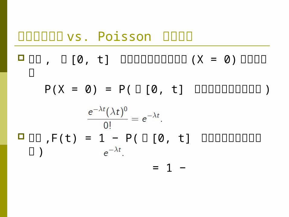
指數隨機變數 vs. Poisson 隨機變數 因此 , 在 [0, t] 的區間內沒有公車抵達 (X = 0)

的機率就是 P(X = 0) = P( 在 [0, t] 的區間內沒有公車抵

達 )

= 從而 ,F(t) = 1 − P( 在 [0, t] 的區間內沒有公車

抵達 ) = 1 −

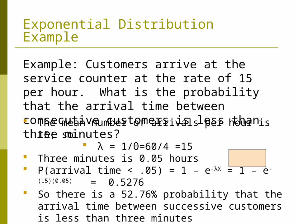
Exponential Distribution Example

Example: Customers arrive at the service counter at the rate of 15 per hour. What is the probability that the arrival time between consecutive customers is less than three minutes? The mean number of arrivals per hour is 15, so

λ = 1/θ=60/4 =15 Three minutes is 0.05 hours P(arrival time < .05) = 1 – e-λX = 1 – e-(15)(0.05) =

0.5276 So there is a 52.76% probability that the arrival

time between successive customers is less than three minutes

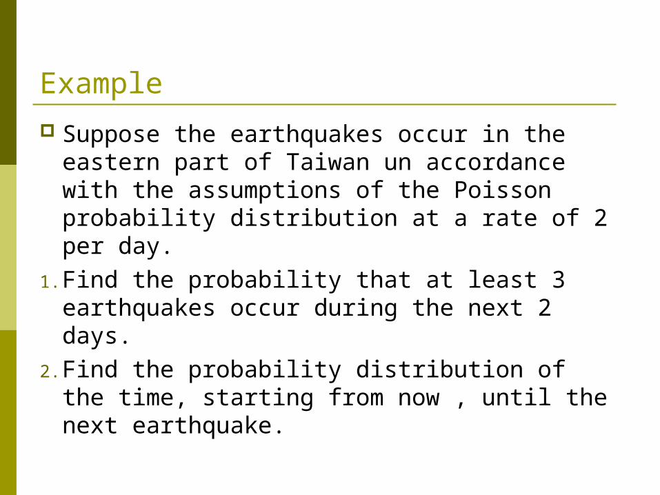
Example

Suppose the earthquakes occur in the eastern part of Taiwan un accordance with the assumptions of the Poisson probability distribution at a rate of 2 per day.

1. Find the probability that at least 3 earthquakes occur during the next 2 days.

2. Find the probability distribution of the time, starting from now , until the next earthquake.

Example

Ans:1. λ = 2 次 / 天 表示在未來兩天發生地震的次數

tX

42*2

)(~

t

tPX ot

2

0

44

131!

41)2(1)3(

x

x

tt ex

eXPXP

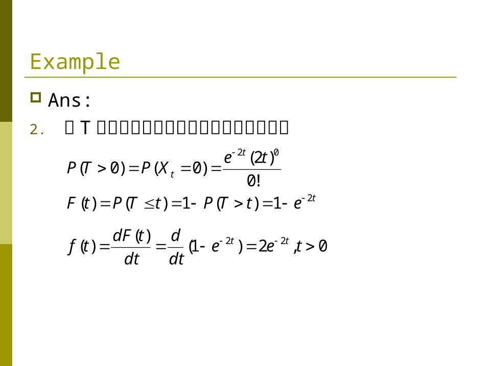
Example

Ans:2. 令 T 表從現在開始到下次地震發生所需時間

!0

)2()0()0(

02 teXPTP

t

t

tetTPtTPtF 21)(1)()(

0,2)1()(

)( 22 teedt

d

dt

tdFtf tt

常態分配 (normal distribution) 又稱 Gaussian分配 (Gaussian distribution) 。這是因為德國數學家 Johann Carl Friedrich Gauss (1777–1855) 在常態分配的發展歷史中 , 佔有決定性的地位

Gauss 導出了常態分配作為量測誤差的機率分配。到了十九世紀中葉 , 常態分配已被視為自然界各種觀察所必見的分配 , 在大多數的情況下 , 觀測值資料的次數分配 (empirical distribution) 多近似於常態分配 , 是故此分配以「常態」命名之

Johann Carl Friedrich Gauss (1777–1855)

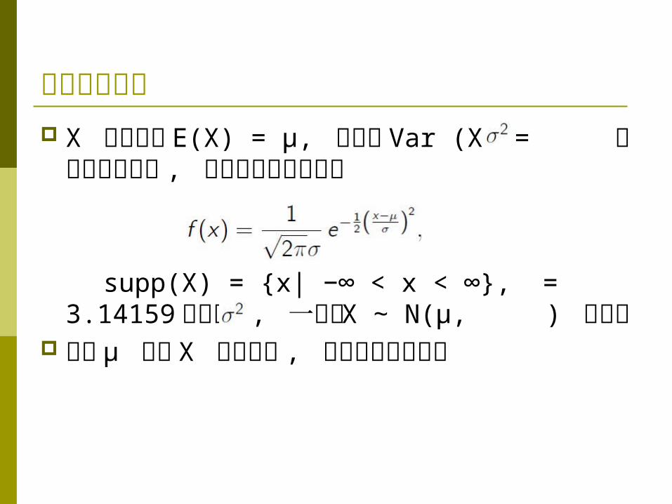
常態隨機變數 X 為期望值 E(X) = μ, 變異數 Var (X) = 的

常態隨機變數 , 若其機率密度函數為

supp(X) = {x| −∞ < x < ∞}, = 3.14159 為圓周率 , 一般以 X ∼ N(μ, ) 表示之

參數 μ 既是 X 的期望值 , 也是中位數與眾數

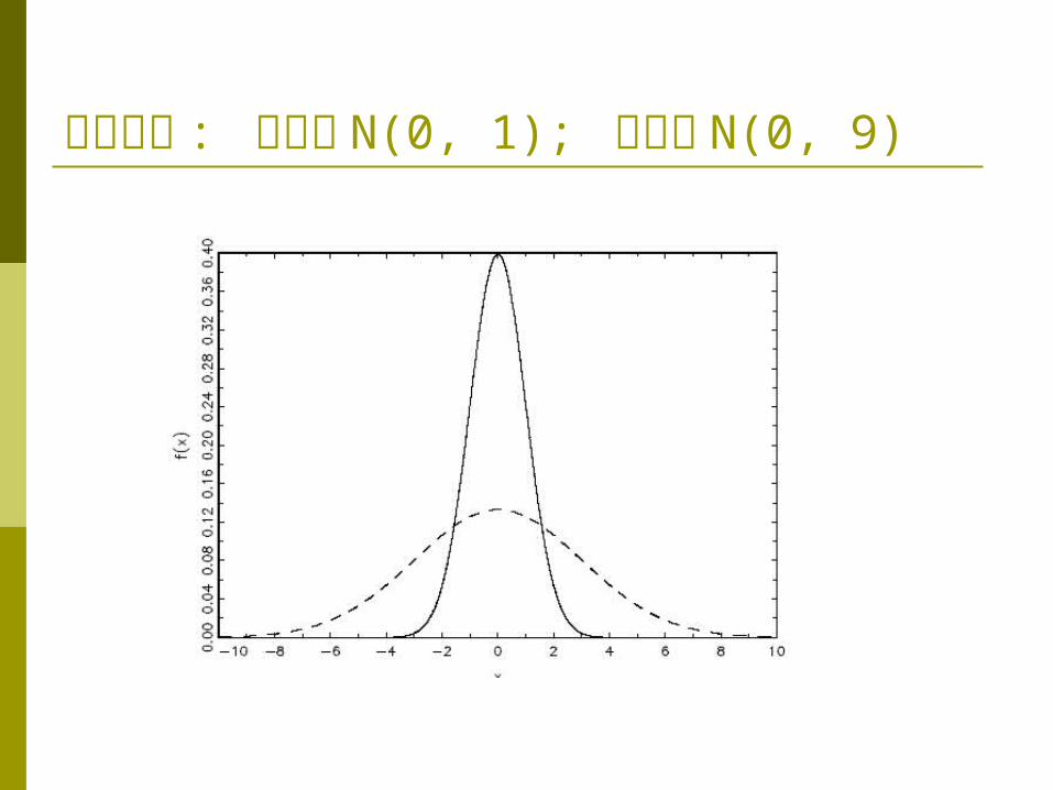
常態分配 : 實線為 N(0, 1); 虛線為 N(0, 9)

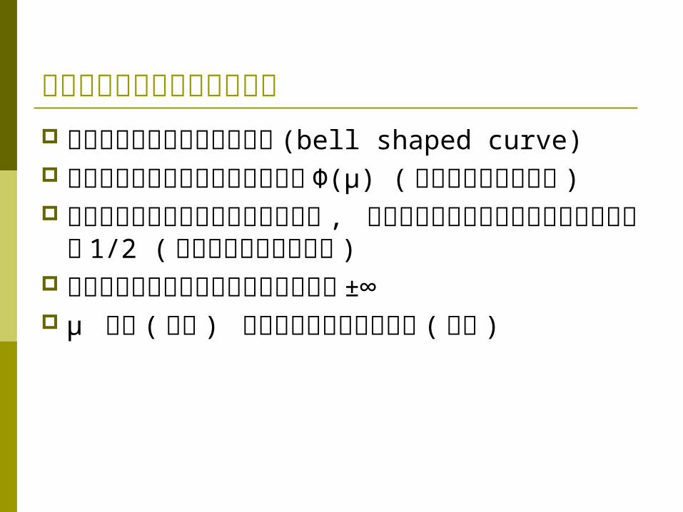
有關常態分配的幾個重要事實 常態分配機率密度函數為鐘型 (bell shaped

curve) 常態分配機率密度函數的最大值為 Φ(μ) ( 亦即期

望值等於眾數 ) 常態分配機率密度函數對稱於期望值 , 期望值左右兩側密度函數下的面積分別為 1/2 ( 亦即期望值等於中位數 )

常態分配機率密度函數尾端部分趨近於 ±∞ μ 增加 (減少 ) 使整個機率密度函數右移 (左

移 )

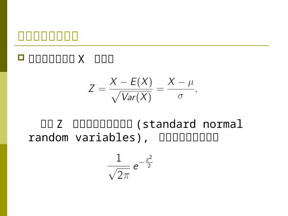
標準常態隨機變數 將常態隨機變數 X 標準化

則稱 Z 為標準常態隨機變數 (standard normal random variables), 具有機率密度函數為

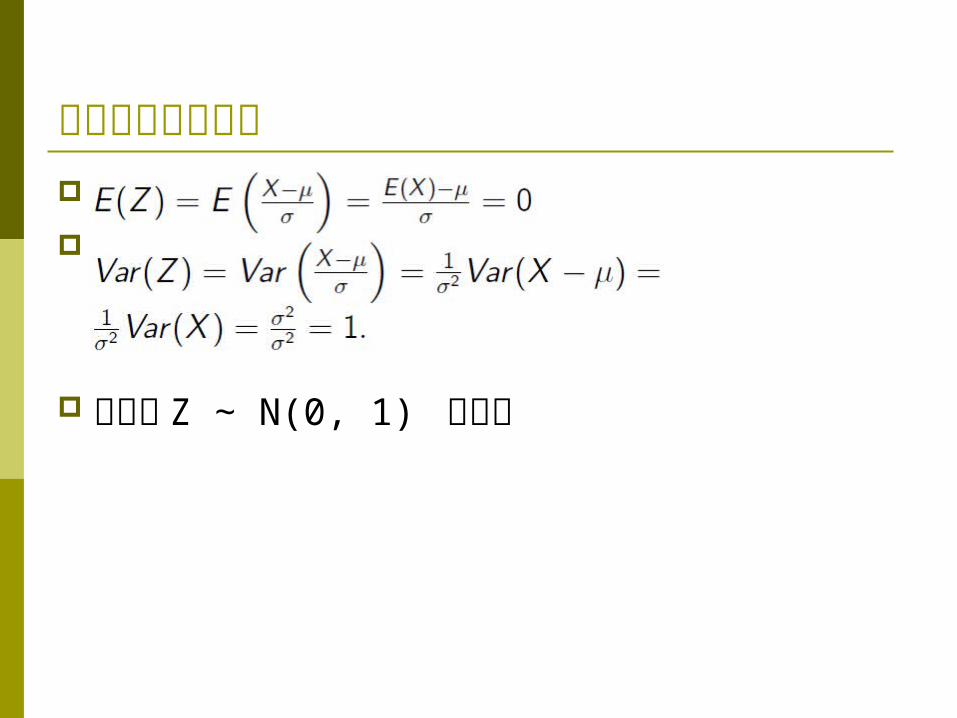
標準常態隨機變數

我們以 Z ∼ N(0, 1) 表示之

我們通常以希臘字母 與 分別代表標準常態隨機變數的機率密度函數與分配函數 :

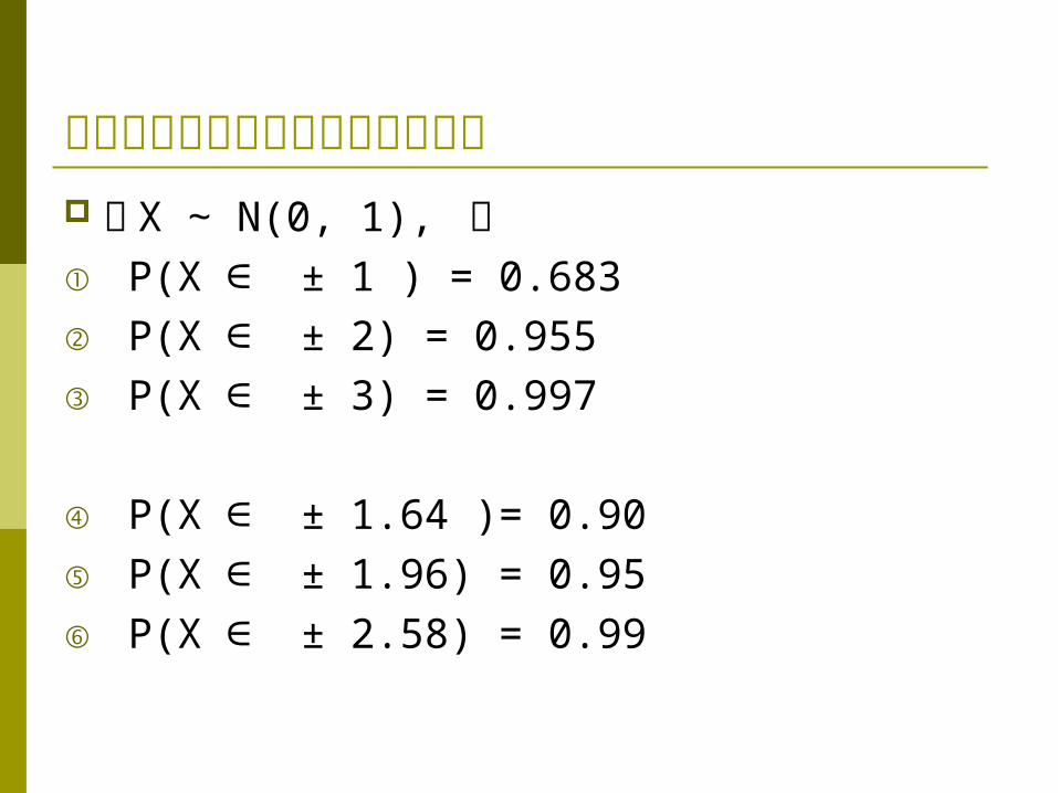
有關標準常態分配的幾個重要數字 若 X ∼ N(0, 1), 則① P(X ∈ ± 1 ) = 0.683② P(X ∈ ± 2) = 0.955③ P(X ∈ ± 3) = 0.997

④ P(X ∈ ± 1.64 )= 0.90⑤ P(X ∈ ± 1.96) = 0.95⑥ P(X ∈ ± 2.58) = 0.99

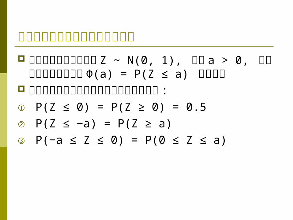
標準常態隨機變數的機率值之計算 對於標準常態隨機變數 Z ∼ N(0, 1), 給定 a >

0, 我們可以透過查表計算Φ(a) = P(Z ≤ a) 的機率值

以下常態分配的對稱性質可以幫助我們查表 :① P(Z ≤ 0) = P(Z ≥ 0) = 0.5② P(Z ≤ −a) = P(Z ≥ a)③ P(−a ≤ Z ≤ 0) = P(0 ≤ Z ≤ a)

Normal Distribution Probability

( ) ( )d

cP c x d f x dx

c dx

f(x)

Probability is area under curve!

Z= 0

= 1

1.96

Z .04 .05

1.8 .4671 .4678 .4686

.4738 .4744

2.0 .4793 .4798 .4803

2.1 .4838 .4842 .4846

The Standard Normal Table: P(0 < z < 1.96)

.06

1.9 .4750

Standardized Normal Probability Table (Portion)

Probabilities

.4750

Shaded area exaggerated

The Standard Normal Table:P(–1.26 z 1.26)

Z = 0

= 1

–1.26

Standardized Normal Distribution

Shaded area exaggerated

.3962

1.26

.3962 P(–1.26 ≤ z ≤ 1.26)

= .3962 + .3962

= .7924

The Standard Normal Table:P(z > 1.26)

Z = 0

= 1Standardized Normal Distribution

1.26

P(z > 1.26)

= .5000 – .3962

= .1038

.3962

.5000

The Standard Normal Table:P(–2.78 z –2.00)

= 1

= 0–2.78 Z–2.00

.4973

.4772

Standardized Normal Distribution

Shaded area exaggerated

P(–2.78 ≤ z ≤ –2.00)

= .4973 – .4772

= .0201

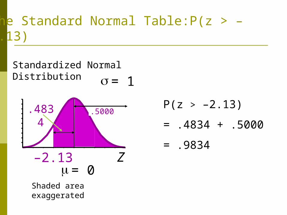
The Standard Normal Table:P(z > –2.13)

Z = 0

= 1

–2.13

Standardized Normal Distribution

Shaded area exaggerated

P(z > –2.13)

= .4834 + .5000

= .9834

.5000.4834

Standardize the Normal Distribution

Normal Distribution

X

One table!

= 0

= 1

Z

Standardized Normal

Distribution

Z= 0

= 1

.12

Standardized Normal

Distribution

Shaded area exaggerated

.0478

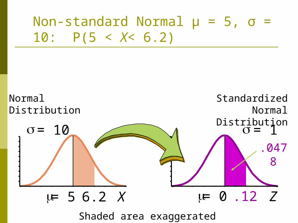
Non-standard Normal μ = 5, σ = 10: P(5 < X< 6.2)

Normal Distribution

X= 5

= 10

6.2

Z = 0

= 1

-.12

Standardized Normal

Distribution

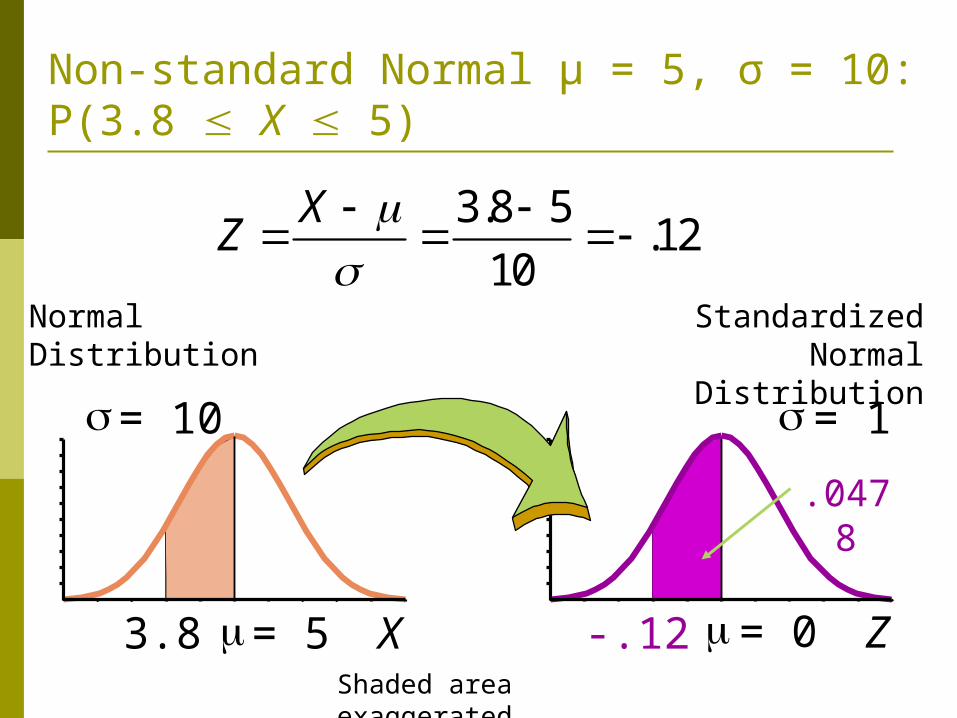
Non-standard Normal μ = 5, σ = 10: P(3.8 X 5)

Normal Distribution

X= 5

= 10

3.8

.0478

Shaded area exaggerated

3.8 5.12

10

XZ

0

= 1

-.21 Z.21

Standardized Normal

Distribution

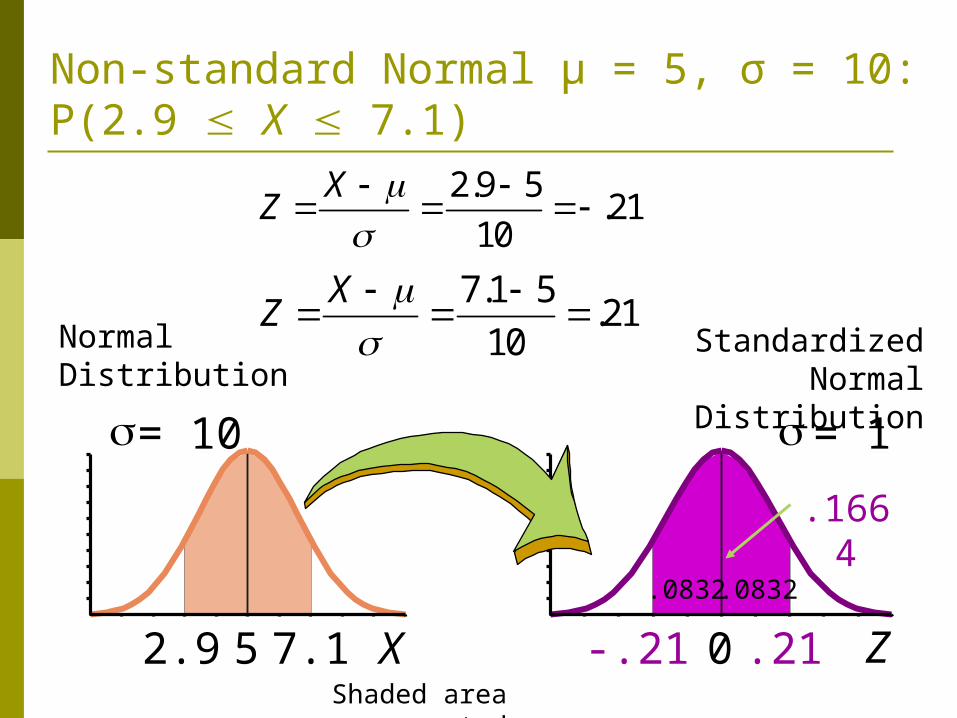
Non-standard Normal μ = 5, σ = 10: P(2.9 X 7.1)

5

= 10

2.9 7.1 X

Normal Distribution

.1664

.0832.0832

Shaded area exaggerated

2.9 5.21

10

XZ

7.1 5.21

10

XZ

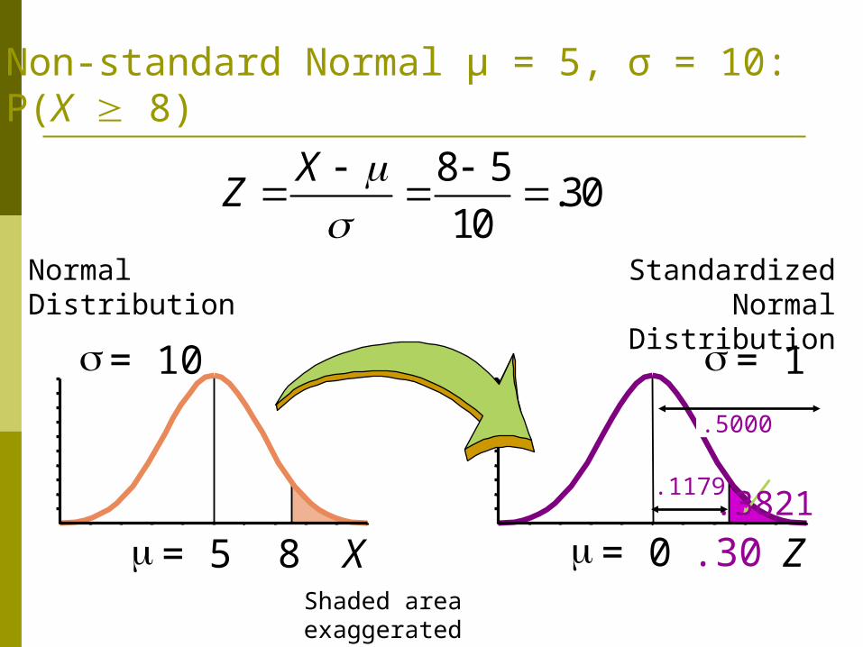
Non-standard Normal μ = 5, σ = 10: P(X 8)

X = 5

= 10

8

Normal Distribution

Z = 0 .30

Standardized Normal

Distribution

= 1

.3821.5000

.1179

Shaded area exaggerated

8 5.30

10

XZ

= 0

= 1

.30 Z.21

Standardized Normal

Distribution

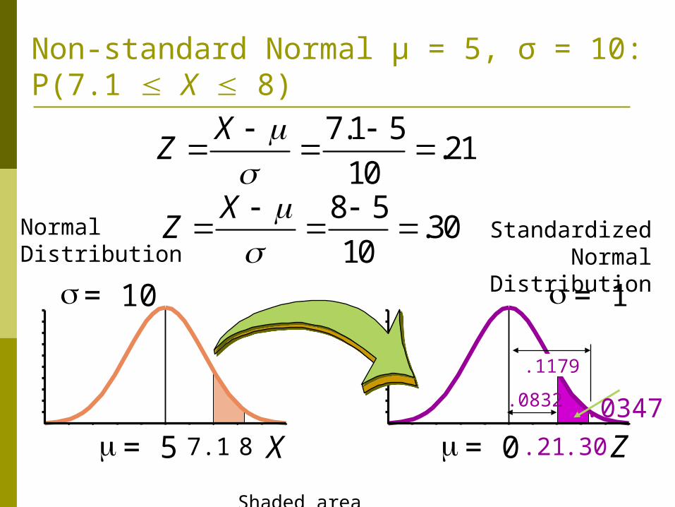
Non-standard Normal μ = 5, σ = 10: P(7.1 X 8)

= 5

= 10

87.1 X

Normal Distribution

.1179 .0347.0832

Shaded area exaggerated

7.1 5.21

10

XZ

8 5.30

10

XZ

例子 : 給定 X ∼ N(5, 64), 試求機率值 P(X ≥ 17)

若 則 因此 ,

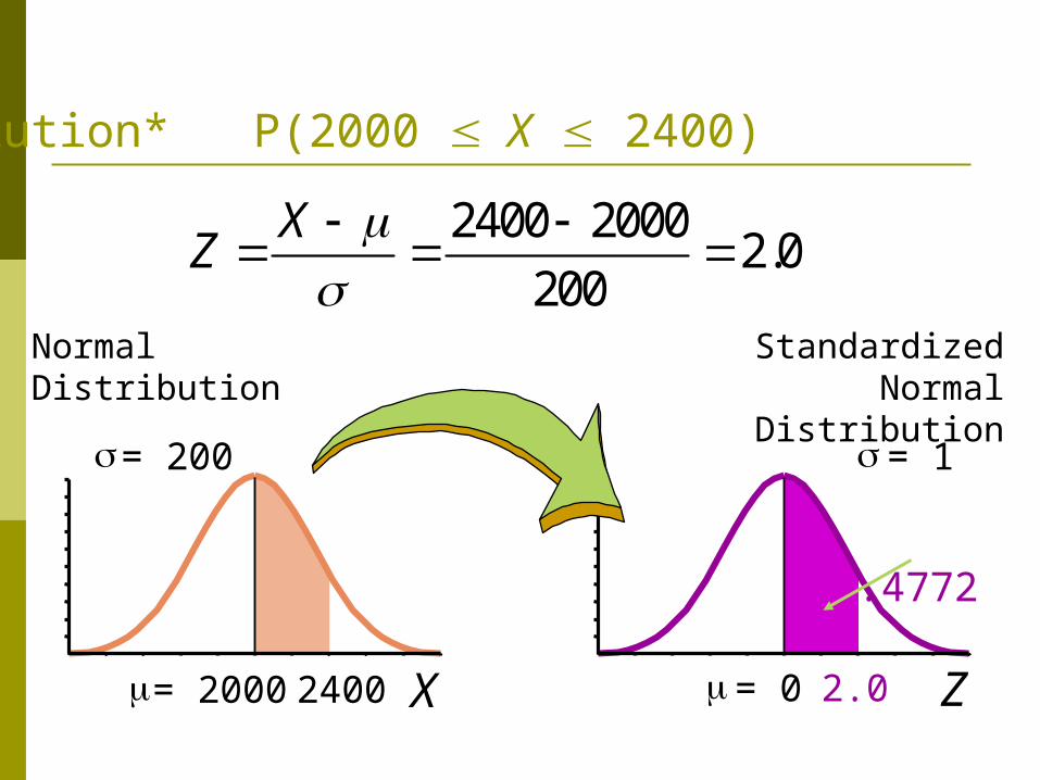
Normal Distribution Thinking Challenge

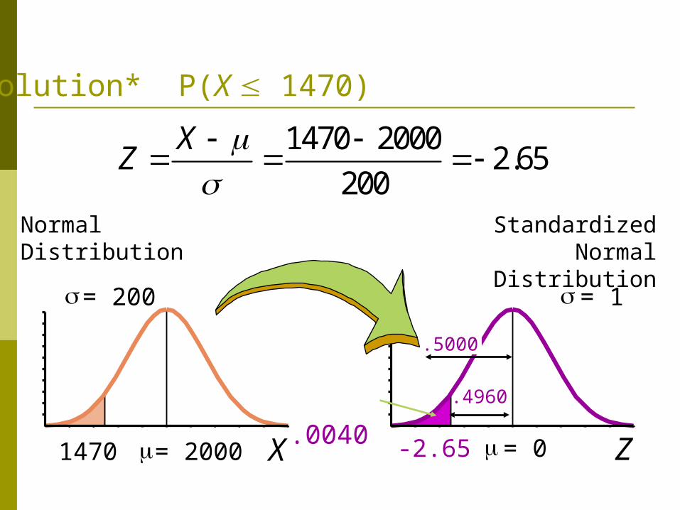
You work in Quality Control for GE. Light bulb life has a normal distribution with = 2000 hours and = 200 hours. What’s the probability that a bulb will last

A. between 2000 and 2400 hours?

B. less than 1470 hours?

Standardized Normal

Distribution

Z = 0

= 1

2.0

Solution* P(2000 X 2400)

Normal Distribution

X = 2000

= 200

2400

.4772

2400 20002.0

200

XZ

Z = 0

= 1

-2.65

Standardized Normal

Distribution

Solution* P(X 1470)

X = 2000

= 200

1470

Normal Distribution

.0040 .4960

.5000

1470 20002.65

200

XZ

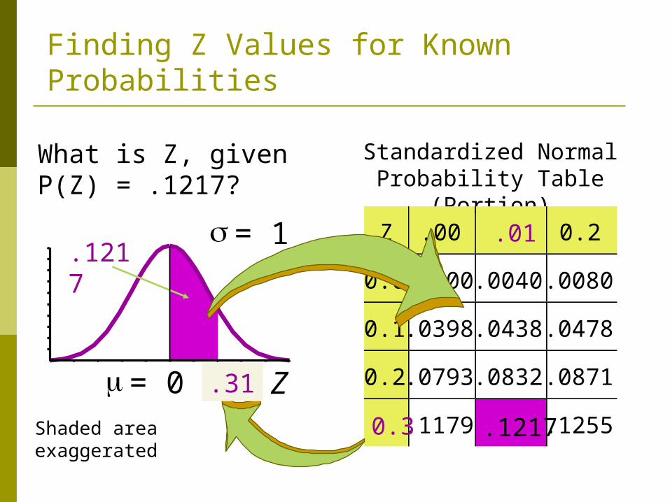
Finding Z Values for Known Probabilities

What is Z, given P(Z) = .1217?

Shaded area exaggerated

Z = 0

= 1

?

.1217

Standardized Normal Probability Table (Portion)

Z .00 0.2

0.0 .0000 .0040 .0080

0.1 .0398 .0438 .0478

0.2 .0793 .0832 .0871

.1179 .1255

.01

0.3 .1217

.31

有關常態分配的幾個重要事實 增加 (減少 ), 使分配更分散 (集中 ), 機率密

度函數越平坦 (陡峭 ) 若 X ∼ N(μ, ), 則① P(X ∈ μ ± σ ) = 0.683② P(X ∈ μ ± 2 σ) = 0.955③ P(X ∈ μ ± 3 σ) = 0.997

Empirical Rules

μ ± 1σ encloses about 68.26% of X’s

f(X)

Xμ μ+1σμ-1σ

What can we say about the distribution of values around the mean? For any normal distribution:

σσ

68.26%

The Empirical Rule

μ ± 2σ covers about 95% of X’s

μ ± 3σ covers about 99.7% of X’s

xμ

2σ 2σ

xμ

3σ 3σ

95.44% 99.73%

常態隨機變數的重要性質 若 X ∼ N(μ, ), 則

這個性質告訴我們常態隨機變數不會隨線性轉換而改變其分配性質。亦即 , 常態隨機變數之線性轉換不變性

常態隨機變數的重要性質若

這個性質告訴我們將獨立的常態隨機變數加總 ,仍為常態隨機變數

若

這是一個常用且重要的性質 , i.i.d. 常態隨機變數的平均數亦為常態隨機變數

更一般化的性質若 為獨立的常態隨機變數 , 且

則

或是

重要性質 若 X, Y 均為常態隨機變數 , 則 X, Y 為獨立的充分且必要條件為

Cov(X, Y) = 0.

一般而言 , X, Y 獨立隱含 X, Y 零相關 , 反之卻不然。然而 , 若 X, Y 均為常態隨機變數 , 則 X, Y 零相關隱含 X, Y 獨立