1 curve fitting ( 曲線適配 ). function approximation 領域技術 trend analysis a process of...
TRANSCRIPT
1
Curve FittingCurve Fitting (( 曲線適配曲線適配 ))
Function Approximation 領域技術
Trend analysis A process of using the pattern of data to make predictions
Function approximation (Chapters 13, 14) Given data of points have noises, find the trend
represented by data • Method of least squares• Minimize the residuals
Function interpolation (Chapters 15, 16) Given precise data of points, find data between these
points Approximating function match the given data exactly
2
3
Curve Fitting: Fitting a Curve Fitting: Fitting a Straight LineStraight Line
Least Square Regression
Regression analysis ( 迴歸分析 ): Statistical technique for estimating the relationships among variables
本單元應習知技巧 Curve fitting Statistics review Linear least square regression Linearization of nonlinear relationships MATLAB 內建指令
4
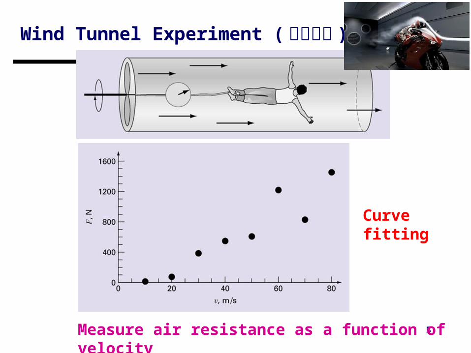
Wind Tunnel Experiment ( 風洞實驗 )
5Measure air resistance as a function of velocity
Curve fitting
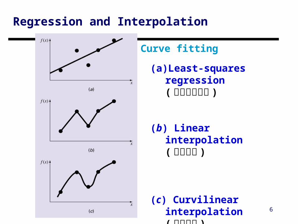
Regression and Interpolation
6
(a) Least-squares regression( 最小平方廻歸 )
(b) Linear interpolation
( 線性內插 )
(c) Curvilinear interpolation( 曲線內插 )
Curve fitting
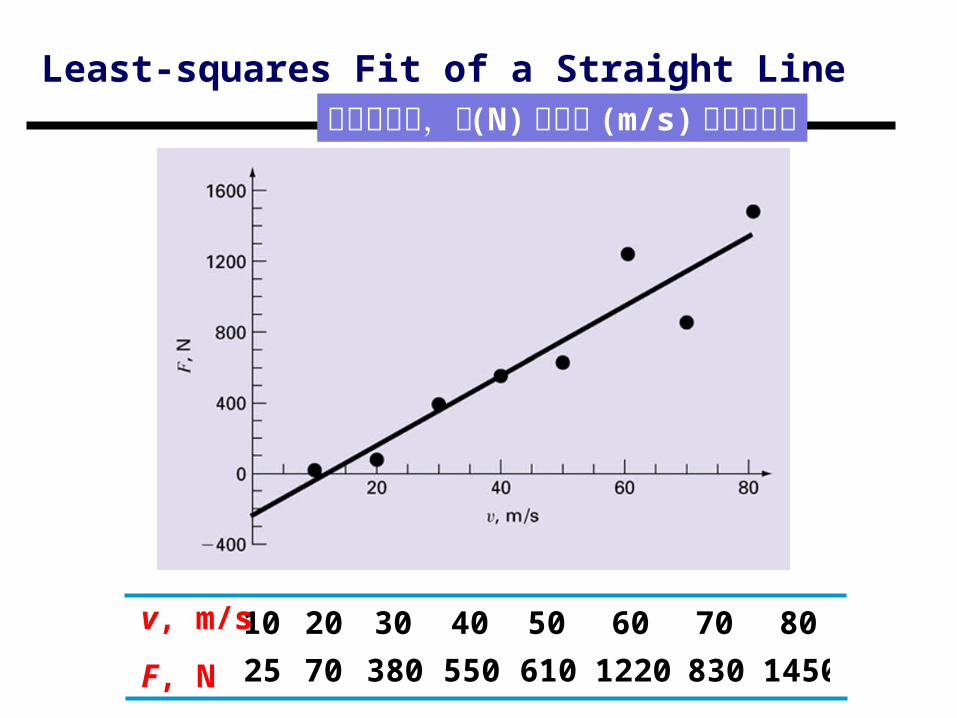
Least-squares Fit of a Straight Line
145083012206105503807025
8070605040302010v, m/s
F, N
風洞實驗中,力 (N) 與速度 (m/s) 的觀測數據
8
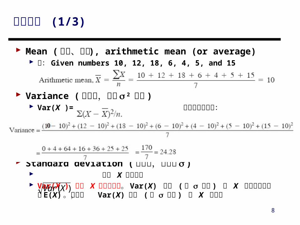
Mean ( 平均、均數 ), arithmetic mean (or average) 例: Given numbers 10, 12, 18, 6, 4, 5, and 15
Variance ( 變異數,常以 2 表示 ) Var(X )= 上例之變異數為:
Standard deviation ( 標準差,常記為 ) 稱為 X 的標準差 Var(X ) 表示 X 的分散程度。 Var(X) 越小 (即 愈小 ) 則 X 越集
中於平均值 E(X)。反之, Var(X) 越大 (即 愈大 ) 則 X 越散開
基本統計 (1/3)
)(XVar

9
自一大小為 N 的母體抽出一組隨機樣本 則樣本平均數 本身亦為隨機變數, 有其機率分配
Sample variance ( 樣本變異數 ) ( 真正的 2未知時可用 ) Unbiased estimate of 2
基本統計 (2/3) :樣本平均數的抽樣分配
nXXX ,,, 21 X
抽自無限母體
nXVar
XE2
)(
)(
nN
nNXVar
XE2
1)(
)(
n
X
n
XXXX in
21
X
抽自有限母體
2
1
)(1
1
n
ii XX
n

基本統計 (3/3) :書例
10
Measurement of the coefficient of thermal expansion of structural steel [106 in/(inF)]
535.6667.6670.6592.6633.6627.6
598.6499.6621.6445.6451.6403.6
703.6542.6659.6624.6733.6662.6
721.6396.6564.6435.6625.6555.6
655.6478.6621.6543.6399.6552.6
667.6325.6495.6775.6554.6485.6
Mean, standard deviation, variance, etc.
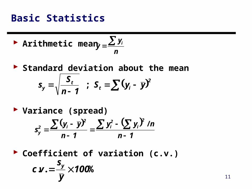
Basic Statistics
Arithmetic mean
Standard deviation about the mean
Variance (spread)
Coefficient of variation (c.v.)
11
n
yy i
2
itt
y yyS 1n
Ss
;
1n
nyy
1n
yys
2
i2i
2i2
y
/
%.. 100y
svc y

1 6.485 0.007173 42.055 2 6.554 0.000246 42.955 3 6.775 0.042150 45.901 4 6.495 0.005579 42.185 5 6.325 0.059875 40.006 6 6.667 0.009468 44.449 7 6.552 0.000313 42.929 8 6.399 0.029137 40.947 9 6.543 0.000713 42.811 10 6.621 0.002632 43.838 11 6.478 0.008408 41.964 12 6.655 0.007277 44.289 13 6.555 0.000216 42.968 14 6.625 0.003059 43.891 15 6.435 0.018143 41.409 16 6.564 0.000032 43.086 17 6.396 0.030170 40.909 18 6.721 0.022893 45.172 19 6.662 0.008520 44.382 20 6.733 0.026669 45.333 21 6.624 0.002949 43.877 22 6.659 0.007975 44.342 23 6.542 0.000767 42.798 24 6.703 0.017770 44.930 25 6.403 0.027787 40.998 26 6.451 0.014088 41.615 27 6.445 0.015549 41.538 28 6.621 0.002632 43.838 29 6.499 0.004998 42.237 30 6.598 0.000801 43.534 31 6.627 0.003284 43.917 32 6.633 0.004008 43.997 33 6.592 0.000498 43.454 34 6.670 0.010061 44.489 35 6.667 0.009468 44.449 36 6.535 0.001204 42.706 236.509 0.406514 1554.198
2i
2i i y yyy i
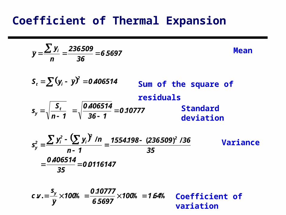
Coefficient of Thermal Expansion
%.%.
.%..
..
/).(./
..
.
..
64110056976
107770100
y
svc
0116147035
4065140
35
365092361981554
1n
nyys
107770136
4065140
1n
Ss
4065140yyS
5697636
509236
n
yy
y
22
i2i2
y
ty
2
it
i
Sum of the square of residuals
Standard deviation
Variance
Coefficient of variation
Mean

Histogram ( 直方圖 )
A histogram depicts the distribution of data For large data set, the histogram often approaches the
normal distribution
14
Normal Distribution
22
1( ) exp
22
x xp x
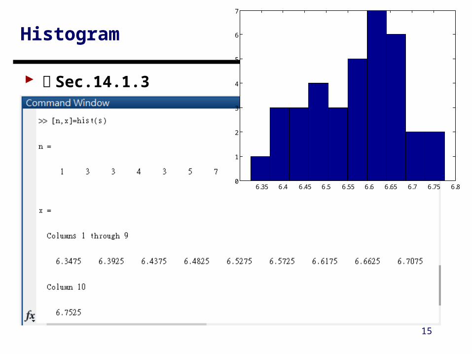
Histogram
書 Sec.14.1.3
15
6.35 6.4 6.45 6.5 6.55 6.6 6.65 6.7 6.75 6.80
1
2
3
4
5
6
7

Regression and Residual
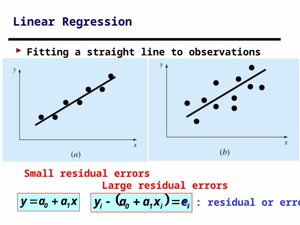
Linear Regression
Fitting a straight line to observations
Small residual errors Large residual errors
xaay 10 ii10i exaay ei : residual or error

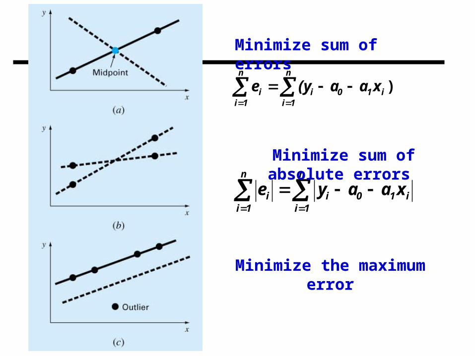
Least Squares ( 最小平方 ) Approximation
Minimizing residuals (errors) minimum average error minimum absolute error minimax error (minimizing the maximum error) least squares (linear, quadratic, ….)
18
)
n
1ii10i
n
1ii xaa(ye
n
1ii10i
n
1ii xaaye
Minimize the maximum error
Minimize sum of errors
Minimize sum of absolute errors
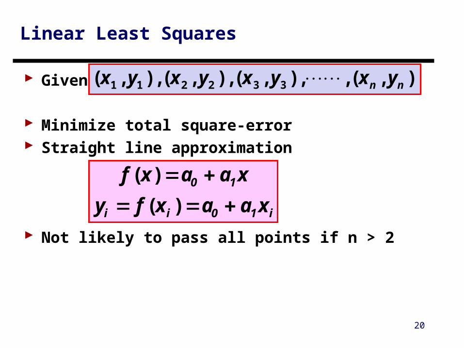
Linear Least Squares
Given
Minimize total square-error Straight line approximation
Not likely to pass all points if n > 2
20
),( , , ),( , ),( , ),( 332211 nn yxyxyxyx
i10ii
10
xaaxfy
xaaxf
)(
)(

Linear Least Squares
Given
Total square-error function: Sum of the squares of the residuals
Minimizing square-error Sr(a0, a1)
21
),( , , ),( , ),( , ),( 332211 nn yxyxyxyx
n
1i
2i10i
n
1i
2ir xaayeS )(
0a
S
0a
S
1
r
0
r
Solve for (a0 , a1)
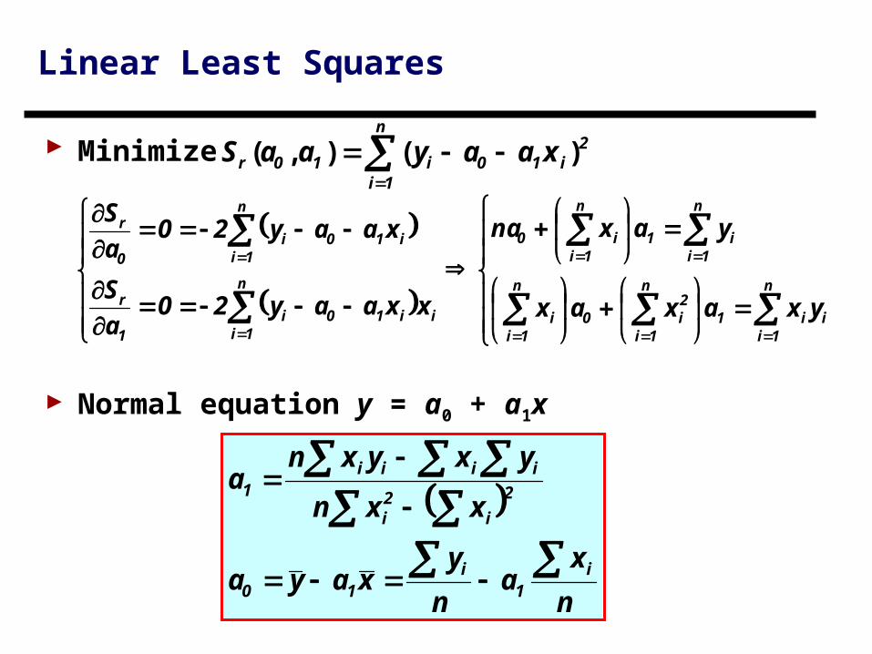
n
1i
2i10i10r xaayaaS )(),(
n
1iii1
n
1i
2i0
n
1ii
n
1ii1
n
1ii0
n
1iii10i
1
r
n
1ii10i
0
r
yxaxax
yaxna
xxaay20a
S
xaay20a
S
n
xa
n
yxaya
xxn
yxyxna
i1
i10
2
i2i
iiii1
Minimize
Normal equation y = a0 + a1x
Linear Least Squares
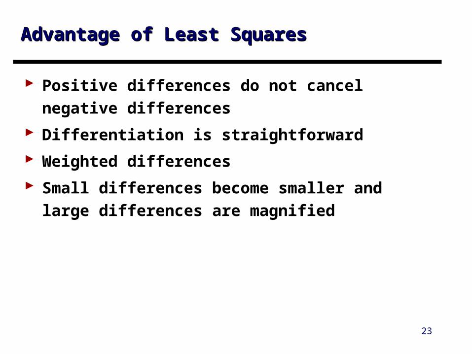
Advantage of Least SquaresAdvantage of Least Squares
Positive differences do not cancel negative
differences
Differentiation is straightforward
Weighted differences
Small differences become smaller and large
differences are magnified
23

Linear Least Squares
Use sum( ) in MATLAB
24
SnS
SSnSa
SnS
SSSSa
S
S
a
a
SS
Sn
yS yxS
xS xS
let
2xxx
yxxy12
xxx
xxyyxx0
xy
y
1
0
xxx
x
n
1iiyi
n
1iixy
n
1iix
n
1i
2ixx
,
,
,,
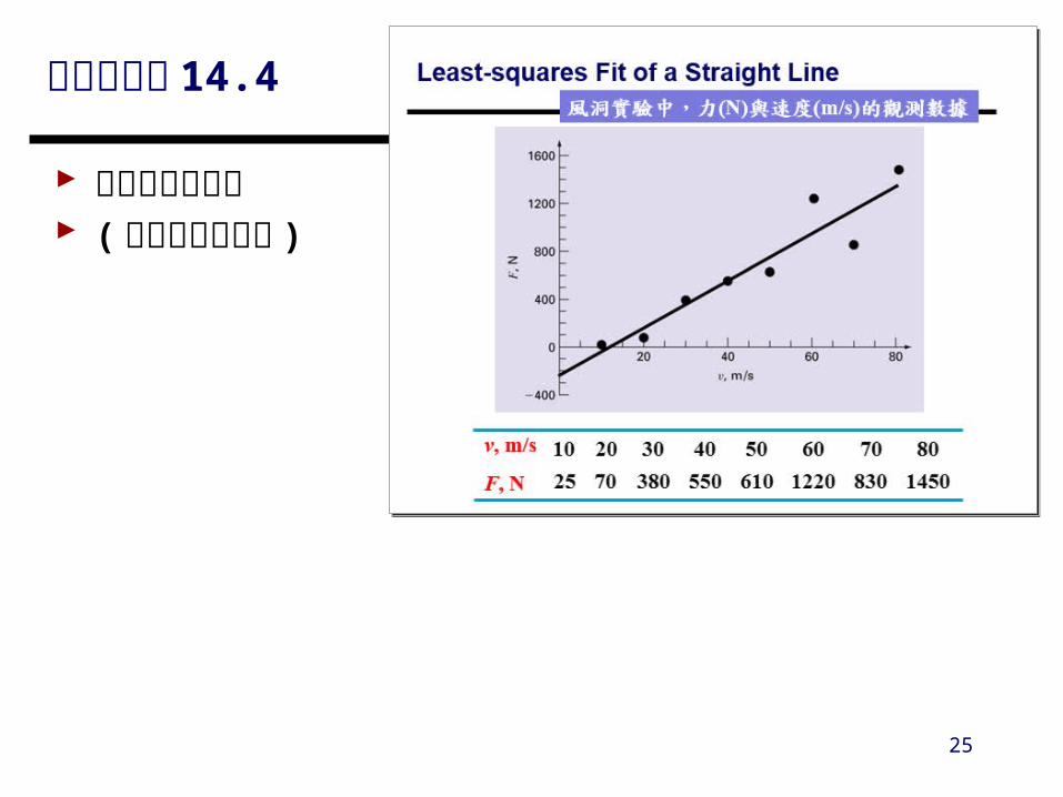
中文書範例 14.4
求最配適的直線 ( 請同學現場操作 )
25

Correlation Coefficient ( 相關係數 )
Sum of squares of the residuals with respect to the mean
Sum of squares of the residuals with respect to the regression line
Coefficient of determination
Correlation coefficient
26
n
ii
n
iit y
ny yyS
1
2
1
1 ;)(
2n
1ii10ir xaayS )(
t
rt
S
SSr
trt SSSr /)(2
完美配適: Sr = 0, r2 = 1 ( 此直線能 100% 解釋數據的變異性 )若 r2=0 則 St = Sr ,代表配適未改善
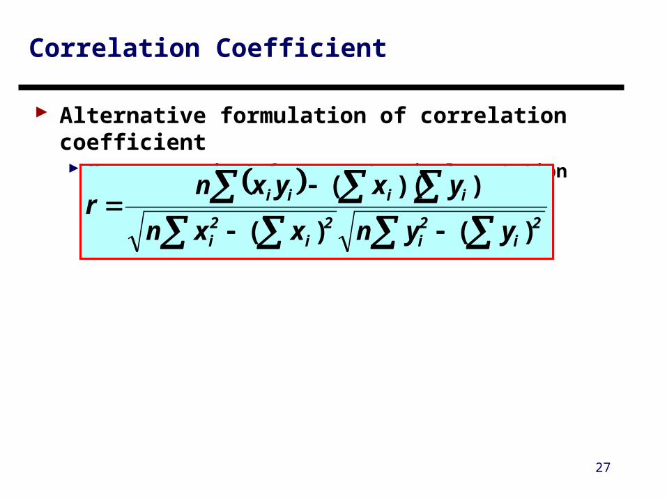
Correlation Coefficient
Alternative formulation of correlation coefficient More convenient for computer implementation
27
2i
2i
2i
2i
iiii
yynxxn
yxyxnr
)()(
))((
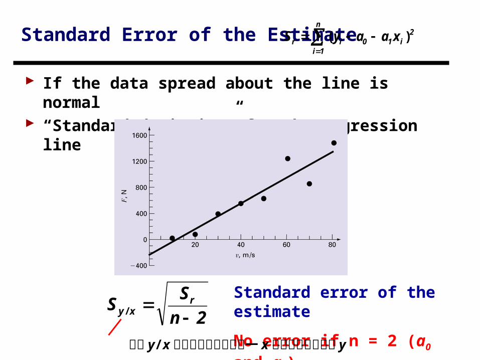
Standard Error of the Estimate
If the data spread about the line is normal “Standard deviation” for the regression line
2n
SS r
xy /
Standard error of the estimate
No error if n = 2 (a0 and a1)
2n
1ii10ir xaayS )(
下標 y/x 代表此誤差是針對某一 x 的預測值所對應的 y

Linear Regression Reduce the Spread of Data
29
Spread of data around the mean
Spread of data around the best-fit line
Normal distributions
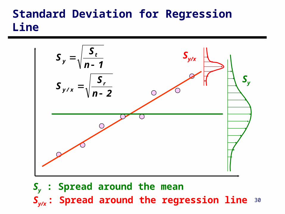
Standard Deviation for Regression Line
30
Sy/x
Sy
Sy : Spread around the mean
Sy/x : Spread around the regression line
2n
SS
1n
SS
rx/y
ty
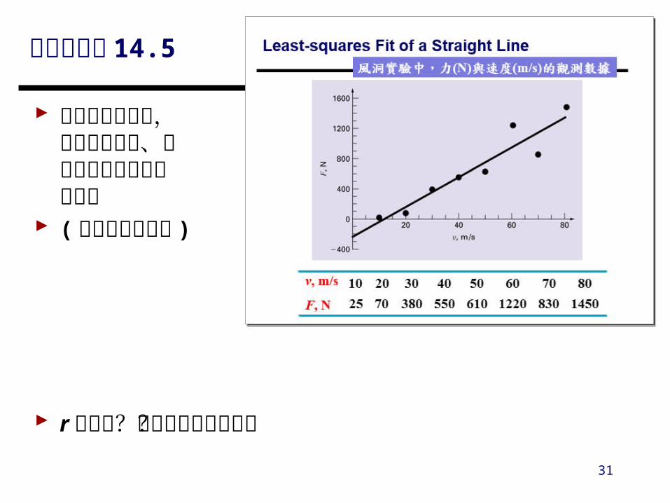
中文書範例 14.5
針對前面的範例,計算總標準差、標準誤差估計以及相關係數
( 請同學現場操作 )
r 值為何?代表的物理意義為?
31
5.119)5.5(7)0.6)(6()5.2)(5(
)0.4)(4()0.2)(3()5.2)(2()5.0)(1(yxS
1407654321xS
24/7n /Sy ; 0.245.50.65.30.40.25.25.0yS
428/7/nSx ; 287654321xS
iixy
22222222ixx
yiy
xix
99112S714322S5119S140S024S28S
199302908453849557
797206122603636066
589600051051725535
326503265001616044
3473004082069023
5625086220054522
1687057658501501
xaayyyyxxyx
rtxyxxyx
2i10i
2iii
2iii
....
....
....
....
....
....
....
....
)()(
另例 (1/2)
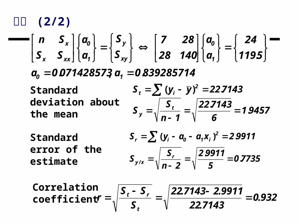
8392857140a 0714285730a
5119
24
a
a
14028
287
S
S
a
a
SS
Sn
10
1
0
xy
y
1
0
xxx
x
.,.
.
945716
714322
1n
SS
714322yyS
ty
2it
..
.)(
Standard deviation about the mean
Standard error of the estimate
773505
99112
2n
SS
99112xaayS
rxy
2i10ir
..
.)(
/
Correlation coefficient 932.0
7143.22
9911.27143.22
S
SSr
t
rt
另例 (2/2)
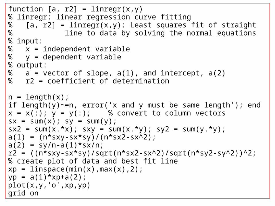
function [a, r2] = linregr(x,y)% linregr: linear regression curve fitting% [a, r2] = linregr(x,y): Least squares fit of straight% line to data by solving the normal equations% input:% x = independent variable% y = dependent variable% output:% a = vector of slope, a(1), and intercept, a(2)% r2 = coefficient of determination
n = length(x);if length(y)~=n, error('x and y must be same length'); endx = x(:); y = y(:); % convert to column vectorssx = sum(x); sy = sum(y);sx2 = sum(x.*x); sxy = sum(x.*y); sy2 = sum(y.*y);a(1) = (n*sxy-sx*sy)/(n*sx2-sx^2);a(2) = sy/n-a(1)*sx/n;r2 = ((n*sxy-sx*sy)/sqrt(n*sx2-sx^2)/sqrt(n*sy2-sy^2))^2;% create plot of data and best fit linexp = linspace(min(x),max(x),2);yp = a(1)*xp+a(2);plot(x,y,'o',xp,yp)grid on
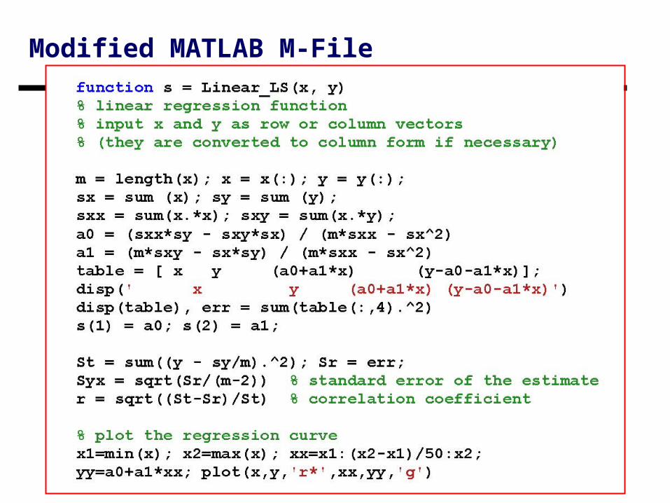
Modified MATLAB M-File
35

» x=1:7x = 1 2 3 4 5 6 7» y=[0.5 2.5 2.0 4.0 3.5 6.0 5.5]y = 0.5000 2.5000 2.0000 4.0000 3.5000 6.0000 5.5000» s=linear_LS(x,y)a0 = 0.0714a1 = 0.8393 x y (a0+a1*x) (y-a0-a1*x) 1.0000 0.5000 0.9107 -0.4107 2.0000 2.5000 1.7500 0.7500 3.0000 2.0000 2.5893 -0.5893 4.0000 4.0000 3.4286 0.5714 5.0000 3.5000 4.2679 -0.7679 6.0000 6.0000 5.1071 0.8929 7.0000 5.5000 5.9464 -0.4464err = 2.9911Syx = 0.7734r = 0.9318s = 0.0714 0.8393 y =0.0714 + 0.8393 x
Sum of squares of residuals Sr
Standard error of the estimate
Correlation coefficient
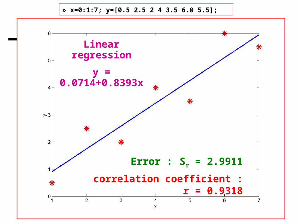
» x=0:1:7; y=[0.5 2.5 2 4 3.5 6.0 5.5];
Linear regression
y = 0.0714+0.8393x
Error : Sr = 2.9911
correlation coefficient : r = 0.9318

function [x,y] = example1
x = [ 1 2 3 4 5 6 7 8 9 10];
y = [2.9 0.5 -0.2 -3.8 -5.4 -4.3 -7.8 -13.8 -10.4 -13.9];
» [x,y]=example1;» s=Linear_LS(x,y)a0 = 4.5933a1 = -1.8570 x y (a0+a1*x) (y-a0-a1*x) 1.0000 2.9000 2.7364 0.1636 2.0000 0.5000 0.8794 -0.3794 3.0000 -0.2000 -0.9776 0.7776 4.0000 -3.8000 -2.8345 -0.9655 5.0000 -5.4000 -4.6915 -0.7085 6.0000 -4.3000 -6.5485 2.2485 7.0000 -7.8000 -8.4055 0.6055 8.0000 -13.8000 -10.2624 -3.5376 9.0000 -10.4000 -12.1194 1.7194 10.0000 -13.9000 -13.9764 0.0764err = 23.1082Syx = 1.6996r = 0.9617s = 4.5933 -1.8570 y = 4.5933 1.8570 x
r = 0.9617

Linear Least Square
y = 4.5933 1.8570 x
Error Sr = 23.1082
Correlation Coefficient r = 0.9617
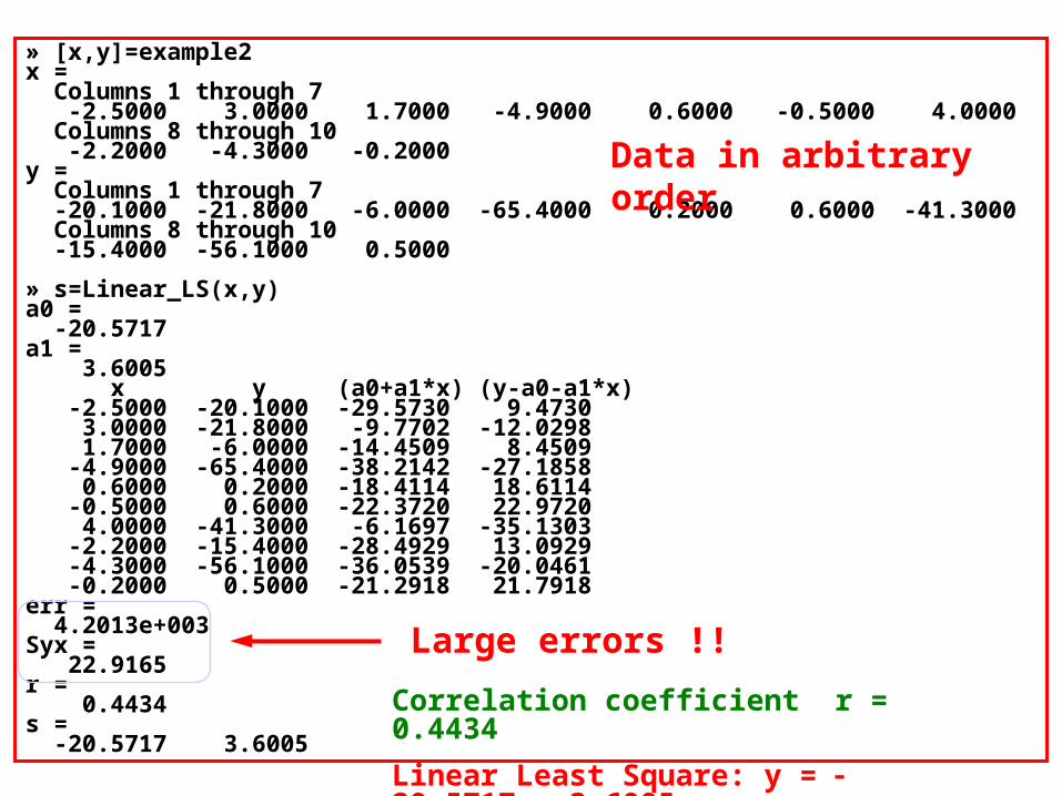
» [x,y]=example2x = Columns 1 through 7 -2.5000 3.0000 1.7000 -4.9000 0.6000 -0.5000 4.0000 Columns 8 through 10 -2.2000 -4.3000 -0.2000y = Columns 1 through 7 -20.1000 -21.8000 -6.0000 -65.4000 0.2000 0.6000 -41.3000 Columns 8 through 10 -15.4000 -56.1000 0.5000
» s=Linear_LS(x,y)a0 = -20.5717a1 = 3.6005 x y (a0+a1*x) (y-a0-a1*x) -2.5000 -20.1000 -29.5730 9.4730 3.0000 -21.8000 -9.7702 -12.0298 1.7000 -6.0000 -14.4509 8.4509 -4.9000 -65.4000 -38.2142 -27.1858 0.6000 0.2000 -18.4114 18.6114 -0.5000 0.6000 -22.3720 22.9720 4.0000 -41.3000 -6.1697 -35.1303 -2.2000 -15.4000 -28.4929 13.0929 -4.3000 -56.1000 -36.0539 -20.0461 -0.2000 0.5000 -21.2918 21.7918err = 4.2013e+003Syx = 22.9165r = 0.4434s = -20.5717 3.6005
Correlation coefficient r = 0.4434
Linear Least Square: y = 20.5717 + 3.6005x
Data in arbitrary order
Large errors !!
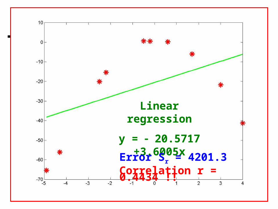
Linear regression
y = 20.5717 +3.6005x
Error Sr = 4201.3Correlation r = 0.4434 !!
Linearization of Nonlinear Relationships
非線性關係的線性化 線性迴歸分析是為數據配適最佳直線的常用技巧,但前提是應變
數與自變數之間的關係為線性 使用迴歸分析之前,應先將數據繪出,以目測決定是否可運用線
性模型• 下一單元將介紹多項式迴歸技巧
一些情境可透過“轉換”的方式,把數據表示成可以匹配線性迴歸的形式
42

Linearization of Nonlinear Relationships
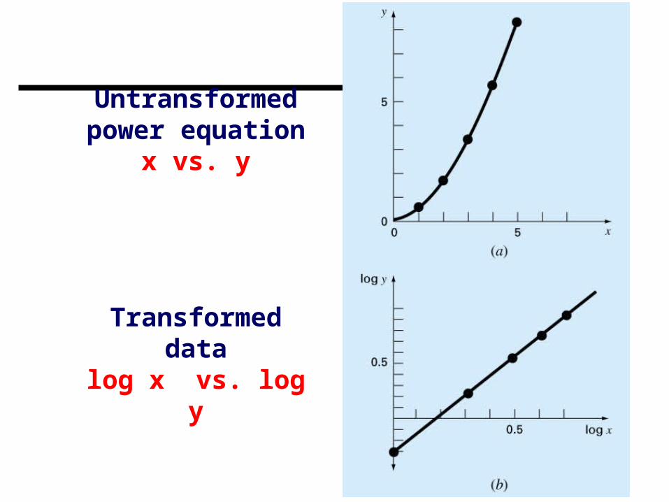
Untransformed power equation
x vs. y
Transformed datalog x vs. log y
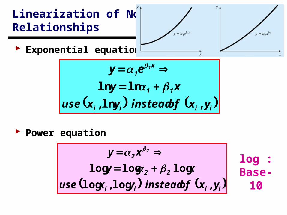
iiii
11
x1
yx of instead yx use
xy
ey 1
,ln,
lnln
iiii
22
2
yx of instead yx use
x y
xy 2
,log,log
logloglog
log : Base-10
Exponential equation
Power equation
Linearization of Nonlinear Relationships

iii
i
4444
yx of instead y
1x use
xy
1
x
1y
,,
iiii
3
3
333
yx of instead y
1
x
1 use
x
11
y
1
x
xy
,,
Saturation-growth-rate equation
Rational function
Linearization of Nonlinear Relationships
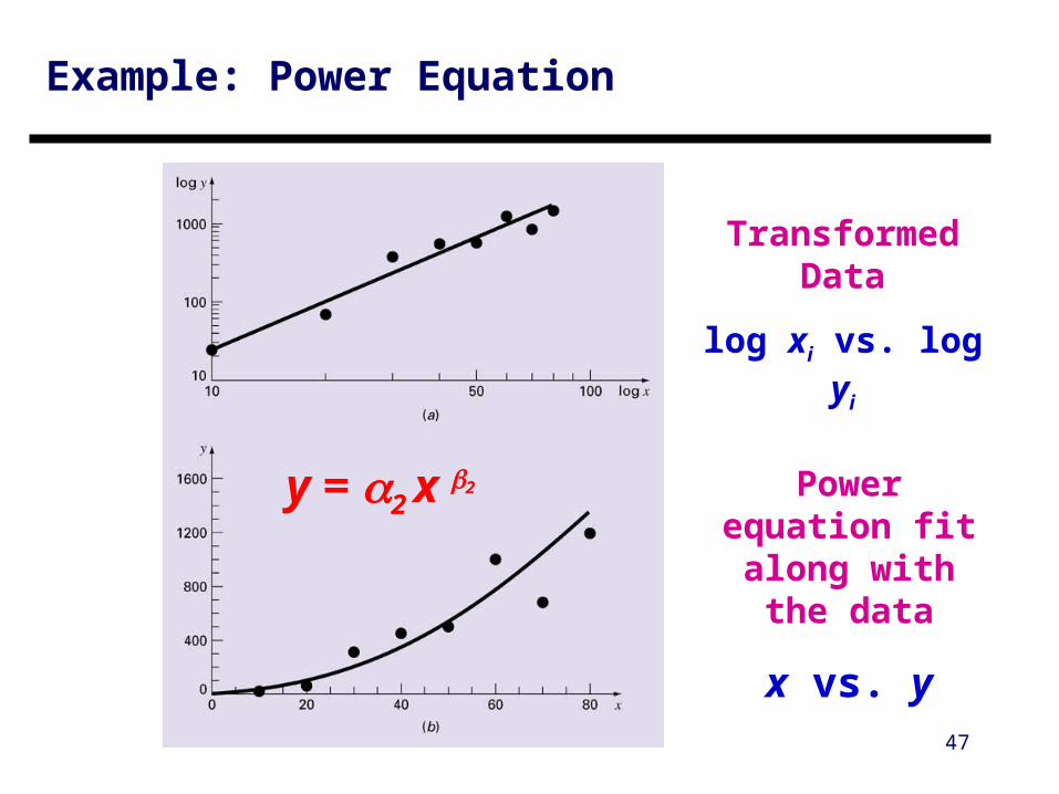
Example: Power Equation
47
Power equation fit along with the data
x vs. y
Transformed Data
log xi vs. log yi
y = 2 x 2
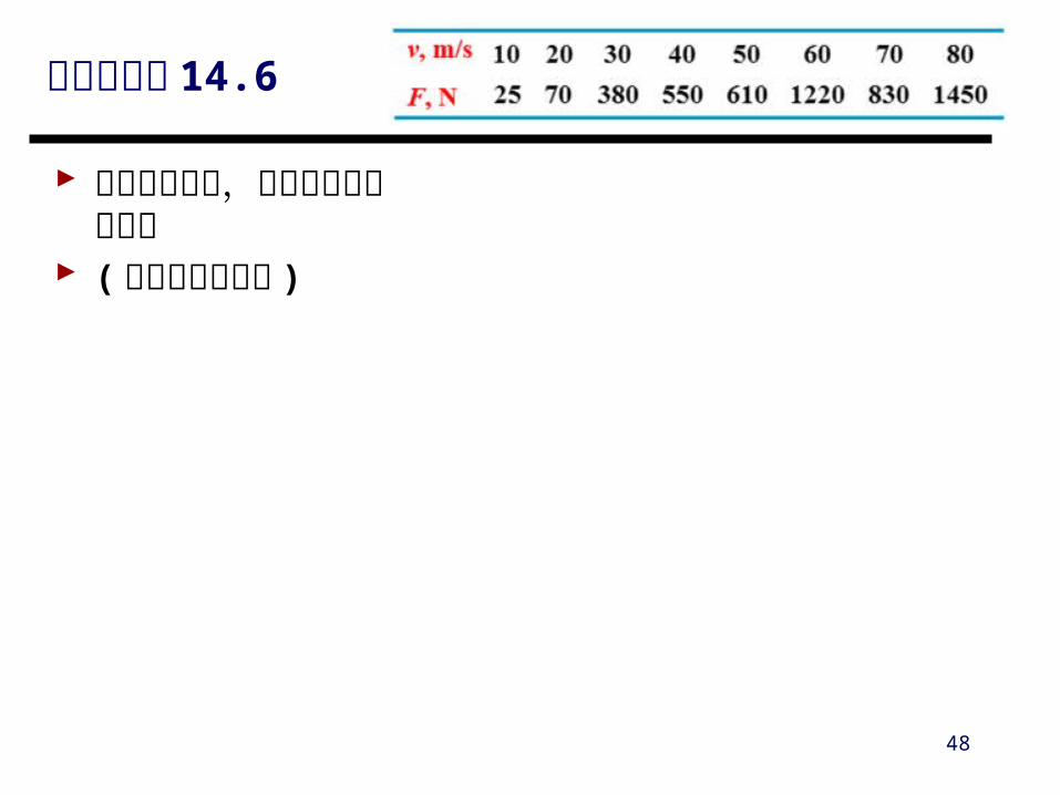
中文書範例 14.6
使用對數轉換,求配適方程式關係數
( 請同學現場操作 )
48
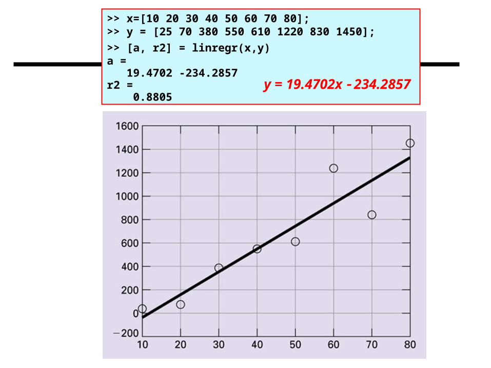
>> x=[10 20 30 40 50 60 70 80];>> y = [25 70 380 550 610 1220 830 1450];
>> [a, r2] = linregr(x,y)a = 19.4702 -234.2857r2 = 0.8805
y = 19.4702x 234.2857
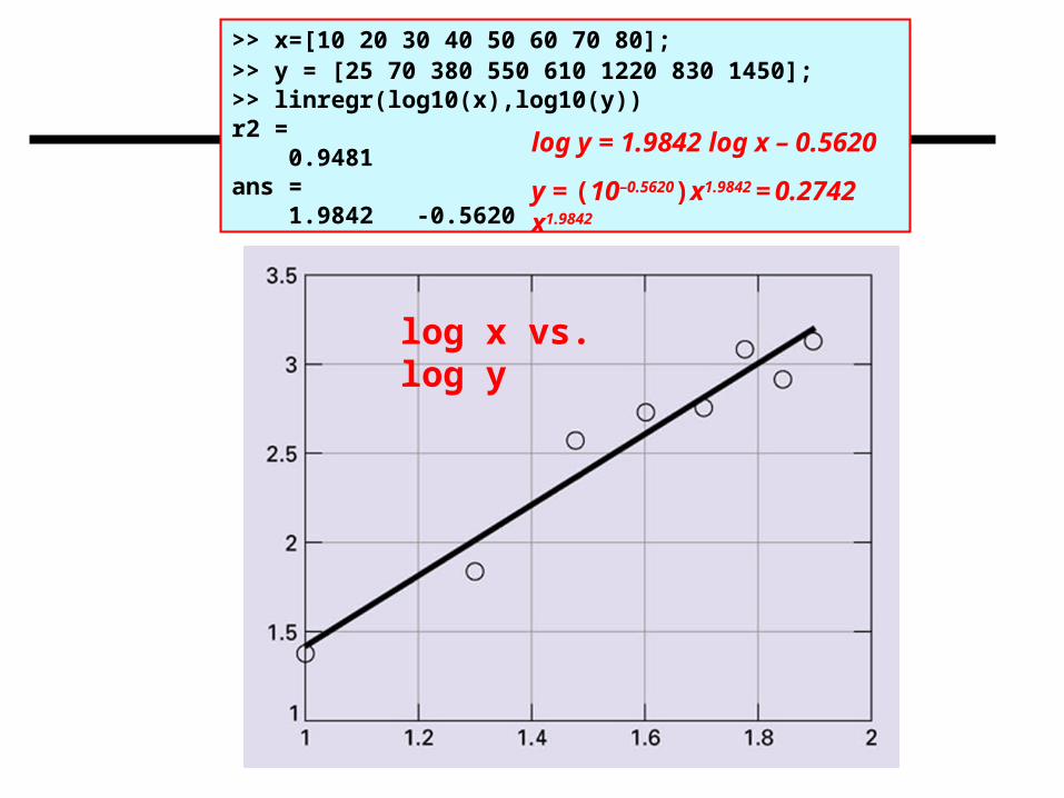
>> x=[10 20 30 40 50 60 70 80];>> y = [25 70 380 550 610 1220 830 1450];>> linregr(log10(x),log10(y))r2 = 0.9481ans = 1.9842 -0.5620
log x vs. log y
log y = 1.9842 log x – 0.5620
y = (10–0.5620)x1.9842 = 0.2742 x1.9842
n1n2n
21n
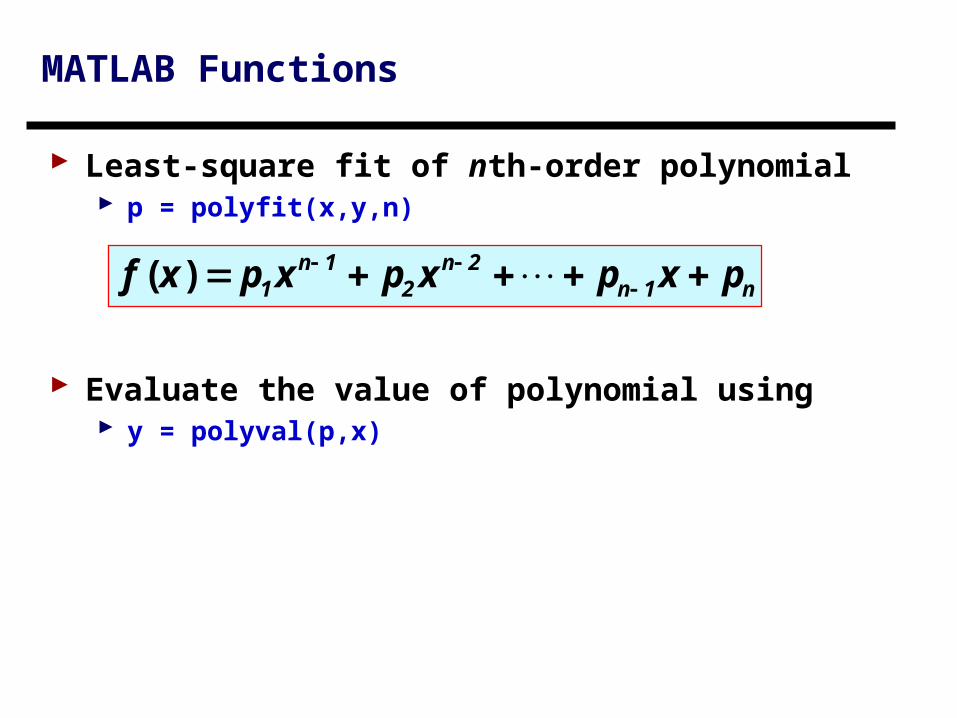
1 pxpxpxpxf )(
Least-square fit of nth-order polynomial p = polyfit(x,y,n)
Evaluate the value of polynomial using y = polyval(p,x)
MATLAB Functions