1 learning objectives when you complete this chapter, you should be able to : identify or define: ...
Post on 20-Dec-2015
218 views
TRANSCRIPT

1
Learning Objectives
When you complete this chapter, you should be able to :
Identify or Define:
Forecasting Forecasting
Types of forecasts Types of forecasts
Time horizons Time horizons
Approaches to forecastsApproaches to forecasts
2
Learning Objectives
When you complete this chapter, you should be able to :
Describe or Explain:
Moving averagesMoving averages
Exponential smoothingExponential smoothing
Trend projectionsTrend projections
Regression and correlation analysisRegression and correlation analysis
Measures of forecast accuracyMeasures of forecast accuracy

3
What is Forecasting?
Process of predicting a future event
??
4
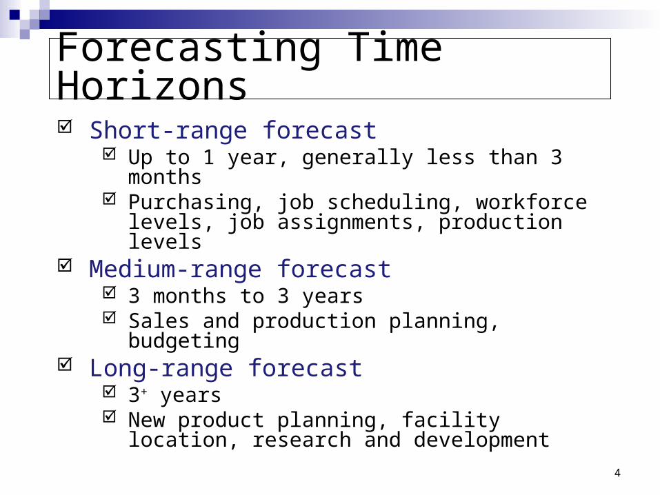
Short-range forecast Up to 1 year, generally less than 3 months Purchasing, job scheduling, workforce levels,
job assignments, production levels Medium-range forecast
3 months to 3 years Sales and production planning, budgeting
Long-range forecast 3+ years New product planning, facility location, research
and development
Forecasting Time Horizons
5
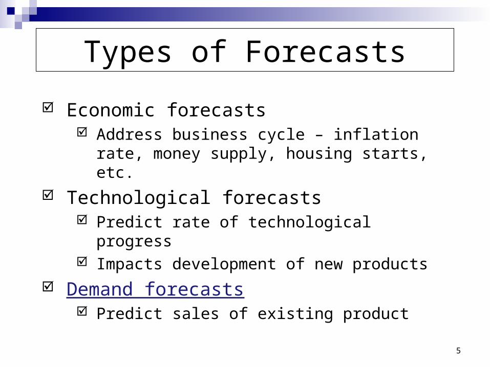
Types of Forecasts
Economic forecasts Address business cycle – inflation rate, money
supply, housing starts, etc.
Technological forecasts Predict rate of technological progress Impacts development of new products
Demand forecasts Predict sales of existing product

6
Strategic Importance of Forecasting
Human Resources – Hiring, training, Human Resources – Hiring, training, laying off workerslaying off workers
Capacity – Capacity shortages can Capacity – Capacity shortages can result in undependable delivery, loss result in undependable delivery, loss of customers, loss of market shareof customers, loss of market share
Supply-Chain Management – Good Supply-Chain Management – Good supplier relations and price advancesupplier relations and price advance
7
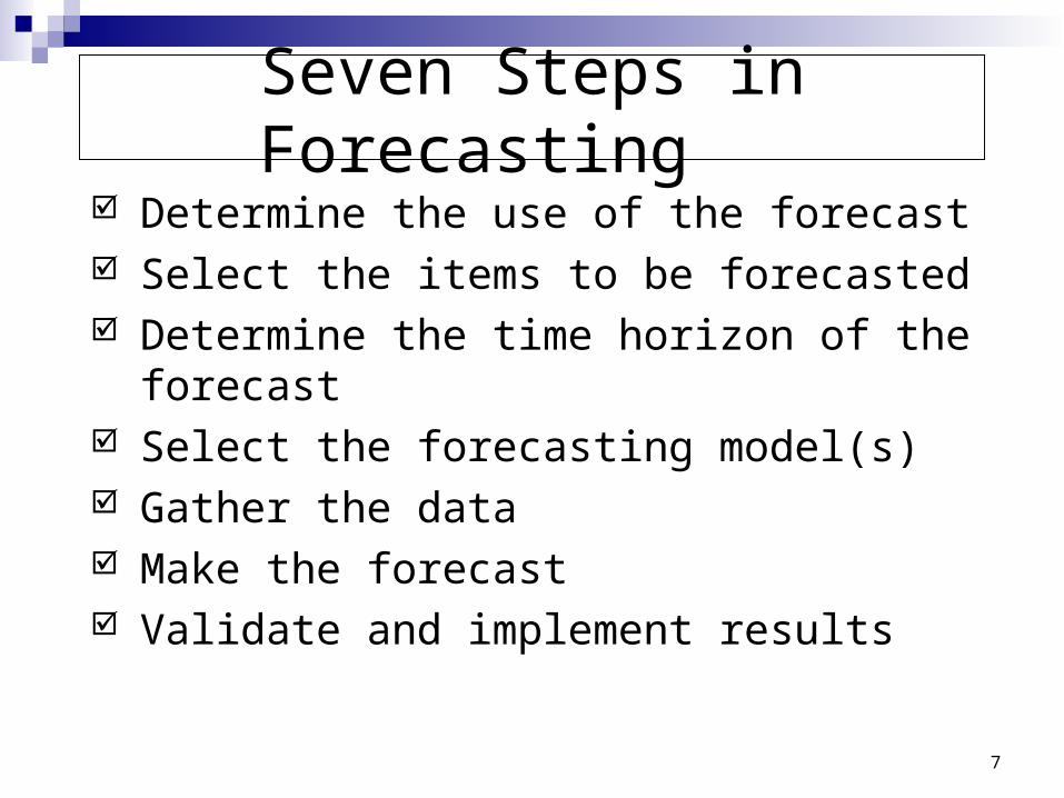
Seven Steps in Forecasting Determine the use of the forecast Select the items to be forecasted Determine the time horizon of the
forecast Select the forecasting model(s) Gather the data Make the forecast Validate and implement results
8
The Realities!
Forecasts are seldom perfectForecasts are seldom perfect
Most techniques assume an Most techniques assume an underlying stability in the systemunderlying stability in the system
Product family and aggregated Product family and aggregated forecasts are more accurate than forecasts are more accurate than individual product forecastsindividual product forecasts

9
Forecasting Approaches
Used when situation is vague and little data exist New products New technology
Involves intuition, experience e.g., forecasting sales on Internet
Qualitative MethodsQualitative Methods
10
Forecasting Approaches
Used when situation is ‘stable’ and historical data exist Existing products Current technology
Involves mathematical techniques e.g., forecasting sales of color
televisions
Quantitative MethodsQuantitative Methods

11
Overview of Qualitative Methods
Jury of executive opinion Pool opinions of high-level executives,
sometimes augment by statistical models Delphi method
Panel of experts, queried iteratively

12
Overview of Qualitative Methods
Sales force composite Estimates from individual salespersons are
reviewed for reasonableness, then aggregated
Consumer Market Survey Ask the customer

13
Involves small group of high-level managers Group estimates demand by working
together Combines managerial experience with
statistical models Relatively quick ‘Group-think’
disadvantage
Jury of Executive Opinion

14
Sales Force Composite
Each salesperson projects his or her sales
Combined at district and national levels
Sales reps know customers’ wants Tends to be overly optimistic

15
Delphi Method
Iterative group process, continues until general agreement is reached
3 types of participants Decision makers Staff Respondents
Staff(Administering
survey)
Decision Makers(Evaluate
responses and make decisions)
Respondents(People who can make valuable
judgments)

16
Consumer Market Survey
Ask customers about purchasing plans
What consumers say, and what they actually do are often different
Sometimes difficult to answer
17
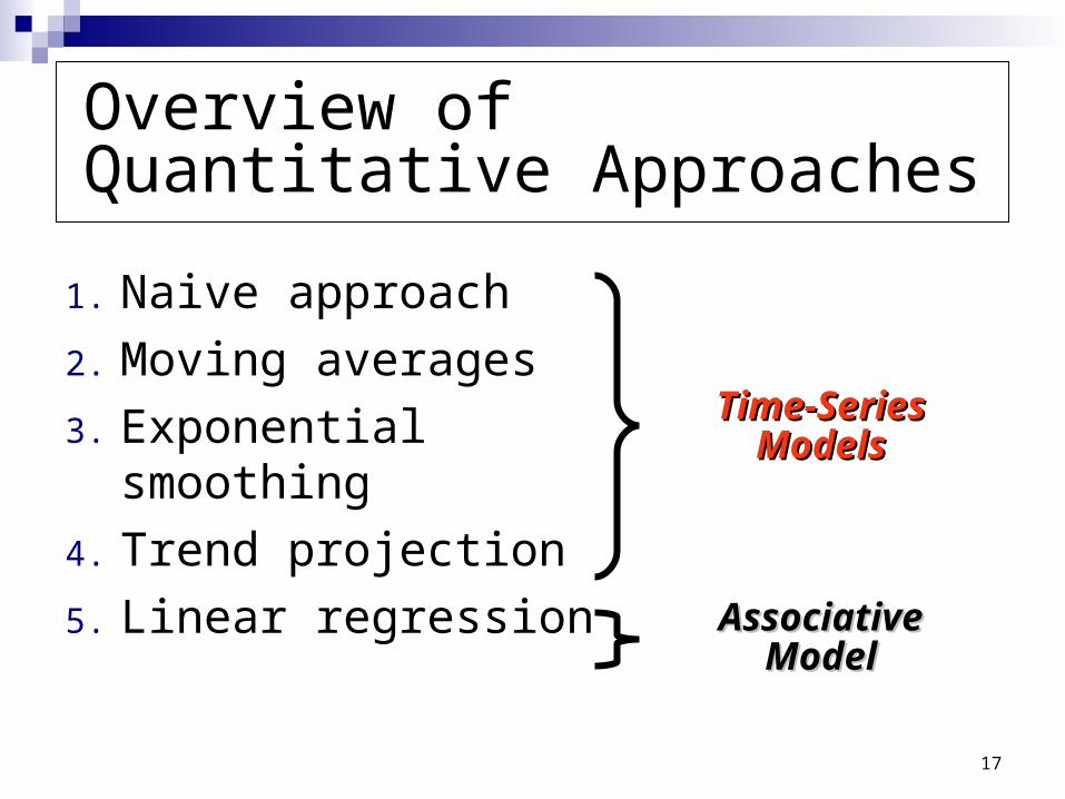
Overview of Quantitative Approaches
1. Naive approach
2. Moving averages
3. Exponential smoothing
4. Trend projection
5. Linear regression
Time-Series Time-Series ModelsModels
Associative Associative ModelModel

18
Set of evenly spaced numerical data Obtained by observing response
variable at regular time periods Forecast based only on past values
Assumes that factors influencing past and present will continue influence in future
Time Series Forecasting
19
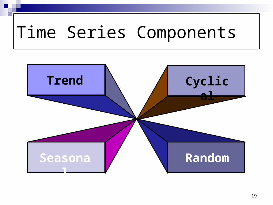
Trend
Seasonal
Cyclical
Random
Time Series Components

20
Components of DemandD
eman
d f
or
pro
du
ct o
r se
rvic
e
| | | |1 2 3 4
Year
Average demand over four years
Seasonal peaks
Trend component
Actual demand
Random variation
Figure 4.1Figure 4.1

21
Persistent, overall upward or downward pattern
Changes due to population, technology, age, culture, etc.
Typically several years duration
Trend Component

22
Regular pattern of up and down fluctuations
Due to weather, customs, etc. Occurs within a single year
Seasonal Component
Number ofPeriod Length Seasons
Week Day 7Month Week 4-4.5Month Day 28-31Year Quarter 4Year Month 12Year Week 52

23
Repeating up and down movements Affected by business cycle, political,
and economic factors Multiple years duration Often causal or
associative relationships
Cyclical Component
00 55 1010 1515 2020
24
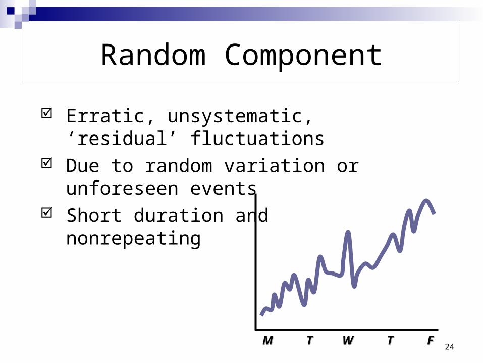
Erratic, unsystematic, ‘residual’ fluctuations
Due to random variation or unforeseen events
Short duration and nonrepeating
Random Component
MM TT WW TT FF
25
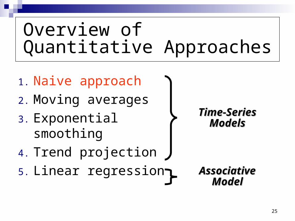
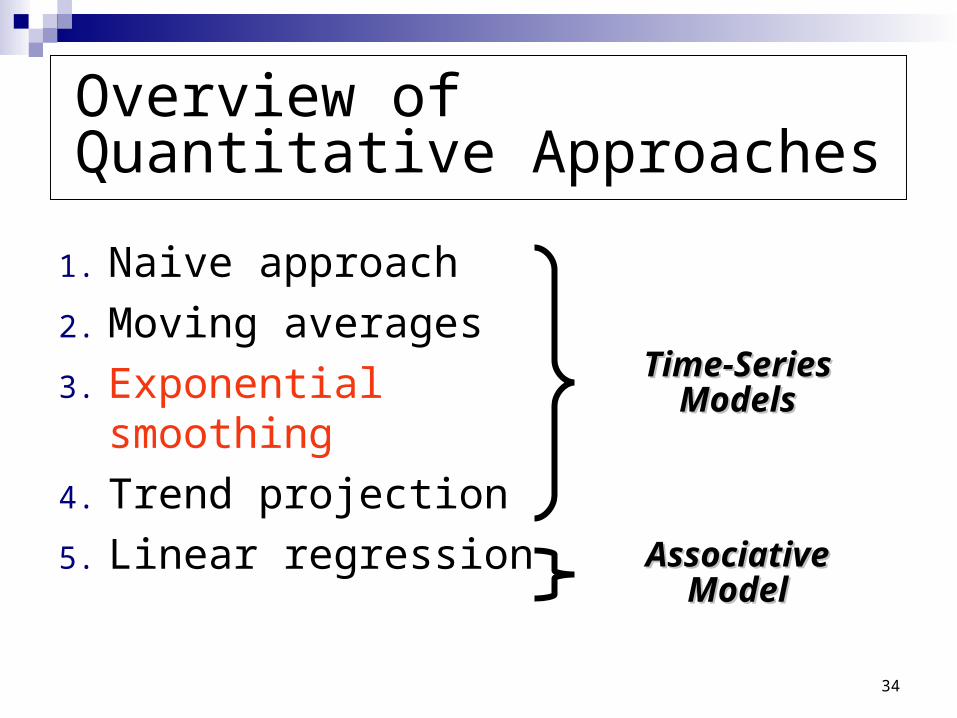
Overview of Quantitative Approaches
1. Naive approach
2. Moving averages
3. Exponential smoothing
4. Trend projection
5. Linear regression
Time-Series Time-Series ModelsModels
Associative Associative ModelModel
26
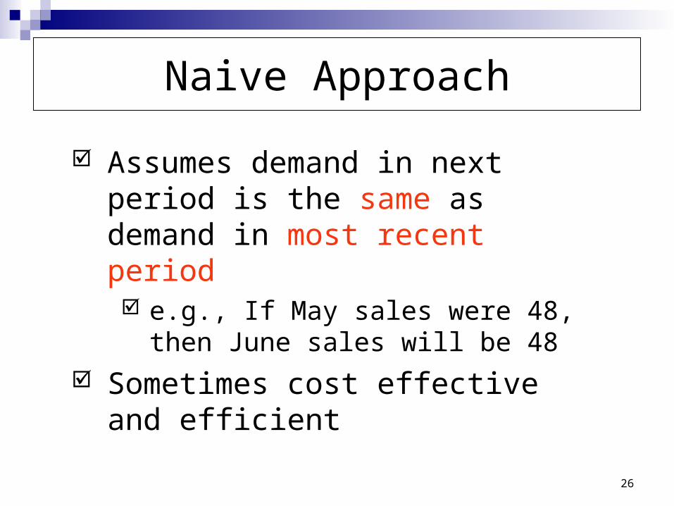
Naive Approach
Assumes demand in next period is the same as demand in most recent period e.g., If May sales were 48, then June
sales will be 48 Sometimes cost effective and
efficient
27
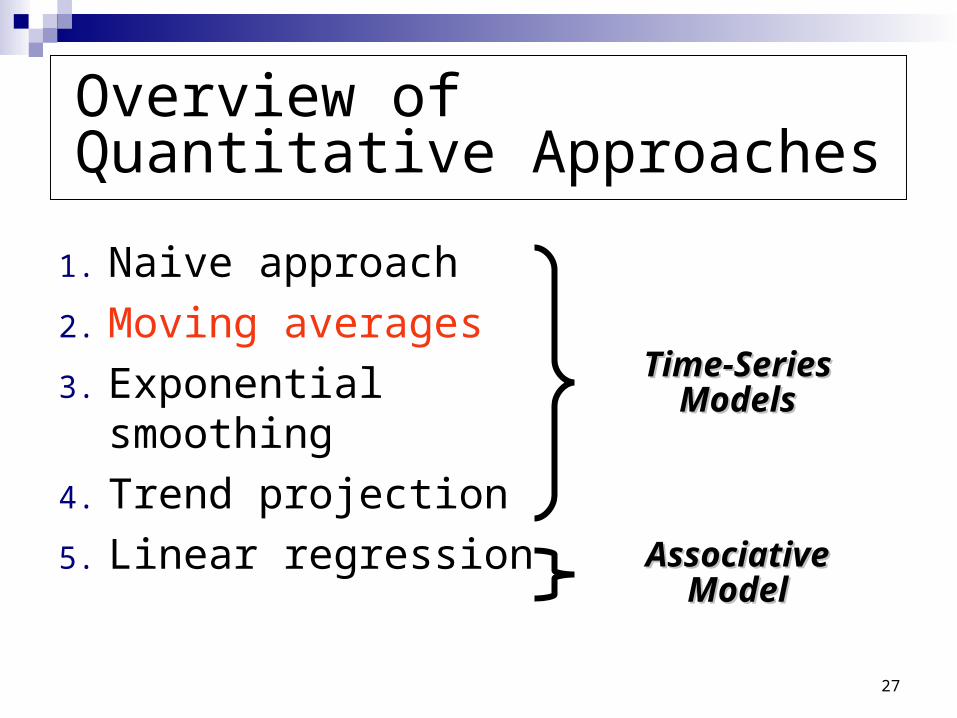
Overview of Quantitative Approaches
1. Naive approach
2. Moving averages
3. Exponential smoothing
4. Trend projection
5. Linear regression
Time-Series Time-Series ModelsModels
Associative Associative ModelModel

28
MA is a series of arithmetic means Used if little or no trend Used often for smoothing
Provides overall impression of data over time
Moving Average Method
Moving averageMoving average ==∑∑ demand in previous n periodsdemand in previous n periods
nn

29
JanuaryJanuary 1010FebruaryFebruary 1212MarchMarch 1313AprilApril 1616MayMay 1919JuneJune 2323JulyJuly 2626
ActualActual 3-Month3-MonthMonthMonth Shed SalesShed Sales Moving AverageMoving Average
(12 + 13 + 16)/3 = 13 (12 + 13 + 16)/3 = 13 22//33
(13 + 16 + 19)/3 = 16(13 + 16 + 19)/3 = 16(16 + 19 + 23)/3 = 19 (16 + 19 + 23)/3 = 19 11//33
Moving Average Example
101012121313
((1010 + + 1212 + + 1313)/3 = 11 )/3 = 11 22//33
30
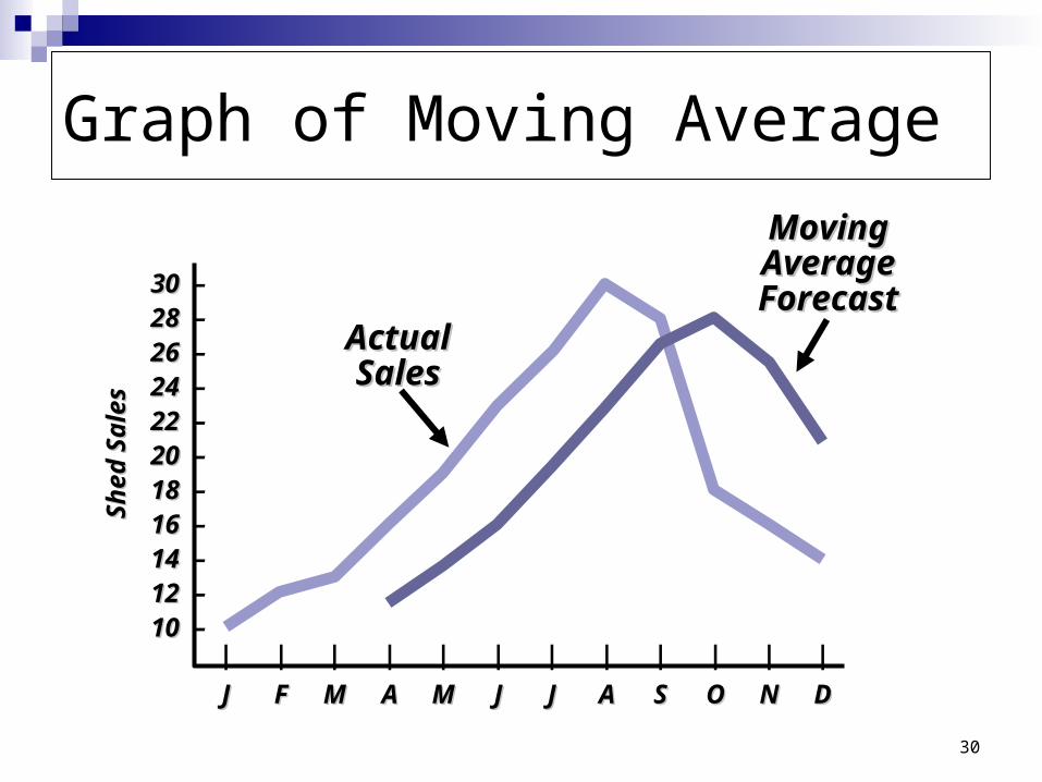
Graph of Moving Average
| | | | | | | | | | | |
JJ FF MM AA MM JJ JJ AA SS OO NN DD
Sh
ed S
ales
Sh
ed S
ales
30 30 –28 28 –26 26 –24 24 –22 22 –20 20 –18 18 –16 16 –14 14 –12 12 –10 10 –
Actual Actual SalesSales
Moving Moving Average Average ForecastForecast

31
Used when trend is present Older data usually less important
Weights based on experience and intuition
Weighted Moving Average
WeightedWeightedmoving averagemoving average ==
∑∑ ((weight for period nweight for period n)) x x ((demand in period ndemand in period n))
∑∑ weightsweights
32
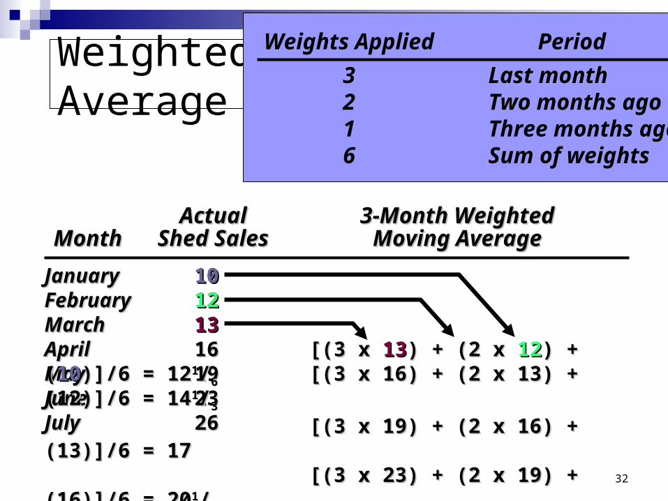
JanuaryJanuary 1010FebruaryFebruary 1212MarchMarch 1313AprilApril 1616MayMay 1919JuneJune 2323JulyJuly 2626
ActualActual 3-Month Weighted3-Month WeightedMonthMonth Shed SalesShed Sales Moving AverageMoving Average
[(3 x 16) + (2 x 13) + (12)]/6 = 14[(3 x 16) + (2 x 13) + (12)]/6 = 1411//33
[(3 x 19) + (2 x 16) + (13)]/6 = 17[(3 x 19) + (2 x 16) + (13)]/6 = 17[(3 x 23) + (2 x 19) + (16)]/6 = 20[(3 x 23) + (2 x 19) + (16)]/6 = 2011//22
Weighted Moving Average
101012121313
[(3 x [(3 x 1313) + (2 x ) + (2 x 1212) + () + (1010)]/6 = 12)]/6 = 1211//66
Weights Applied Period
3 Last month2 Two months ago1 Three months ago6 Sum of weights

33
Moving Average And Weighted Moving Average
30 30 –
25 25 –
20 20 –
15 15 –
10 10 –
5 5 –
Sa
les
de
man
dS
ale
s d
em
and
| | | | | | | | | | | |
JJ FF MM AA MM JJ JJ AA SS OO NN DD
Actual Actual salessales
Moving Moving averageaverage
Weighted Weighted moving moving averageaverage
Figure 4.2Figure 4.2
34
Overview of Quantitative Approaches
1. Naive approach
2. Moving averages
3. Exponential smoothing
4. Trend projection
5. Linear regression
Time-Series Time-Series ModelsModels
Associative Associative ModelModel

35
Exponential Smoothing
New forecast =New forecast = last period’s forecastlast period’s forecast+ + ((last period’s actual demand last period’s actual demand
– – last period’s forecastlast period’s forecast))
FFtt = F = Ft t – 1– 1 + + ((AAt t – 1– 1 - - F Ft t – 1– 1))
wherewhere FFtt == new forecastnew forecast
FFt t – 1– 1 == previous forecastprevious forecast
== smoothing (or weighting) smoothing (or weighting) constant constant (0 (0 1) 1)

36
Exponential Smoothing Example
Predicted demand Predicted demand = 142= 142 Ford Mustangs Ford MustangsActual demand Actual demand = 153= 153Smoothing constant Smoothing constant = .20 = .20

37
Exponential Smoothing Example
Predicted demand Predicted demand = 142= 142 Ford Mustangs Ford MustangsActual demand Actual demand = 153= 153Smoothing constant Smoothing constant = .20 = .20
New forecastNew forecast = 142 + .2(153 – 142)= 142 + .2(153 – 142)
38
Exponential Smoothing Example
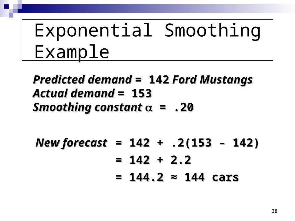
Predicted demand Predicted demand = 142= 142 Ford Mustangs Ford MustangsActual demand Actual demand = 153= 153Smoothing constant Smoothing constant = .20 = .20
New forecastNew forecast = 142 + .2(153 – 142)= 142 + .2(153 – 142)
= 142 + 2.2= 142 + 2.2
= 144.2 ≈ 144 cars= 144.2 ≈ 144 cars
39
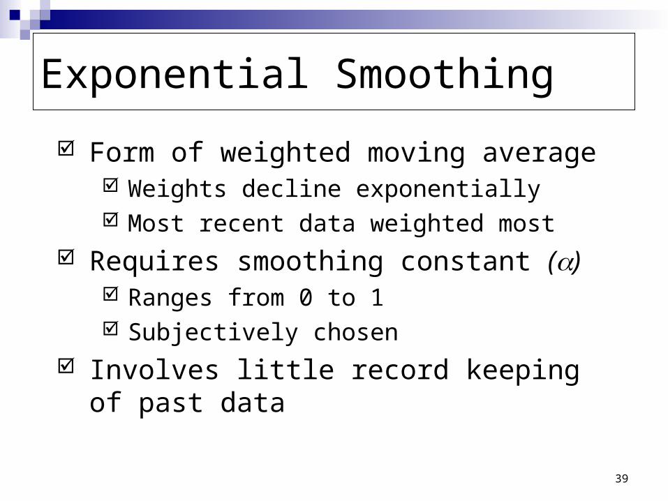
Form of weighted moving average Weights decline exponentially Most recent data weighted most
Requires smoothing constant () Ranges from 0 to 1 Subjectively chosen
Involves little record keeping of past data
Exponential Smoothing
40
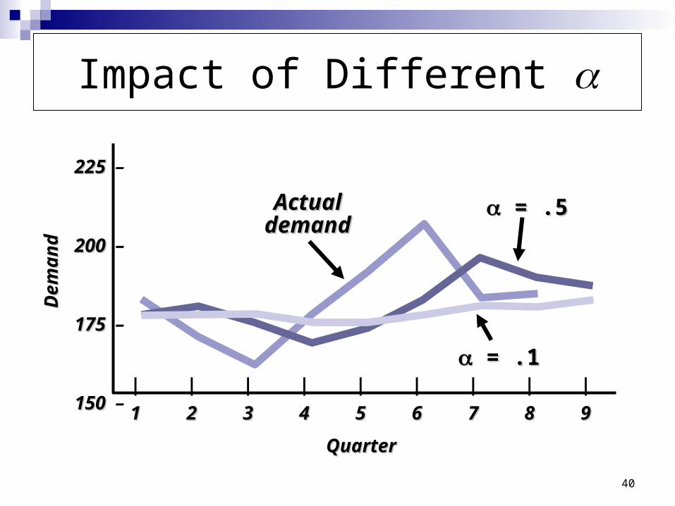
Impact of Different
225 225 –
200 200 –
175 175 –
150 150 –| | | | | | | | |
11 22 33 44 55 66 77 88 99
QuarterQuarter
De
ma
nd
De
ma
nd
= .1= .1
Actual Actual demanddemand
= .5= .5
41
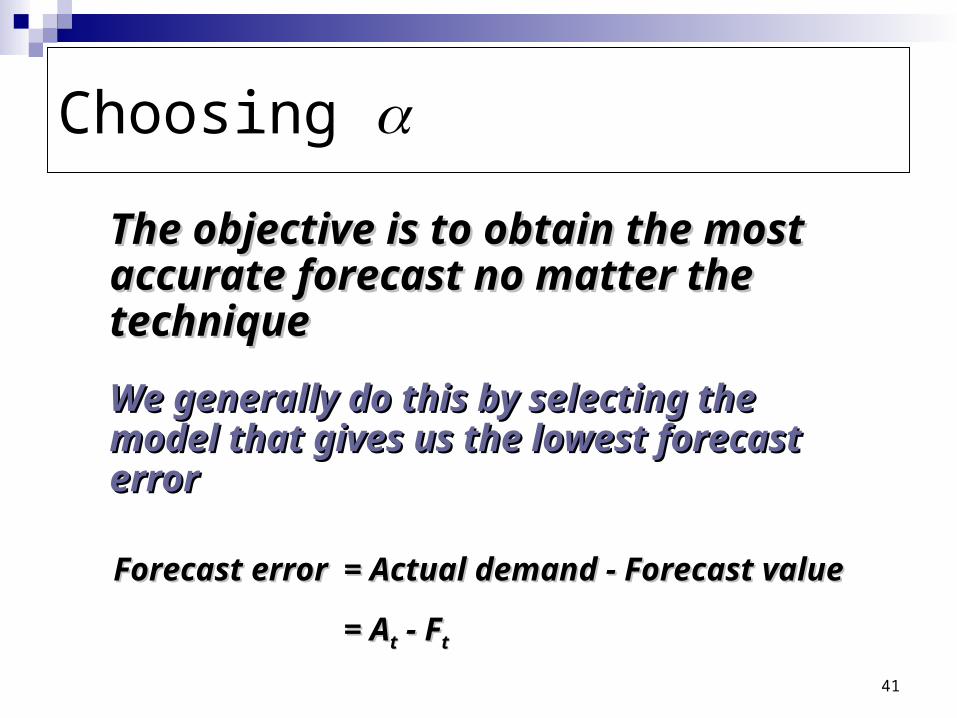
Choosing
The objective is to obtain the most The objective is to obtain the most accurate forecast no matter the accurate forecast no matter the techniquetechnique
We generally do this by selecting the We generally do this by selecting the model that gives us the lowest forecast model that gives us the lowest forecast errorerror
Forecast errorForecast error = Actual demand - Forecast value= Actual demand - Forecast value
= A= Att - F - Ftt
42
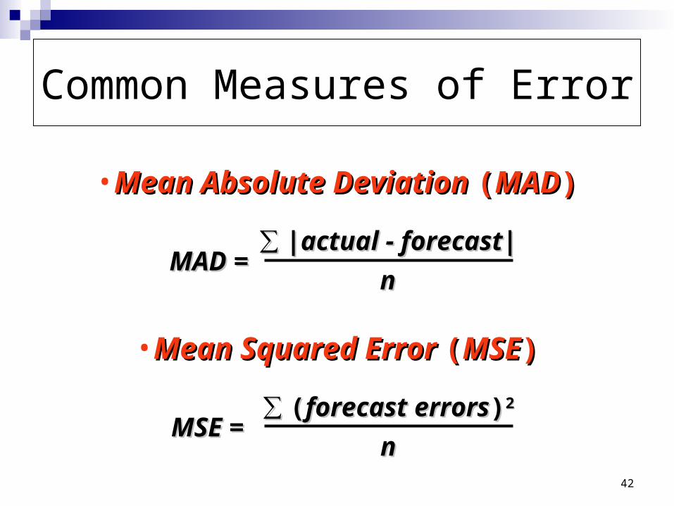
Common Measures of Error
•Mean Absolute Deviation Mean Absolute Deviation ((MADMAD))
MAD =MAD =∑∑ |actual - forecast||actual - forecast|
nn
•Mean Squared Error Mean Squared Error ((MSEMSE))
MSE =MSE =∑∑ ((forecast errorsforecast errors))22
nn

43
Common Measures of Error
Mean Absolute Percent Error Mean Absolute Percent Error ((MAPEMAPE))
MAPE =MAPE =100 100 ∑∑ |actual |actualii - forecast - forecastii|/actual|/actualii
nn
nn
i i = 1= 1
44
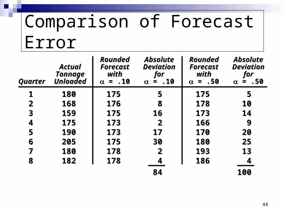
Comparison of Forecast Error
RoundedRounded AbsoluteAbsolute RoundedRounded AbsoluteAbsoluteActualActual ForecastForecast DeviationDeviation ForecastForecast DeviationDeviation
TonnageTonnage withwith forfor withwith forforQuarterQuarter UnloadedUnloaded = .10 = .10 = .10 = .10 = .50 = .50 = .50 = .50
11 180180 175175 55 175175 5522 168168 176176 88 178178 101033 159159 175175 1616 173173 141444 175175 173173 22 166166 9955 190190 173173 1717 170170 202066 205205 175175 3030 180180 252577 180180 178178 22 193193 131388 182182 178178 44 186186 44
8484 100100

45
Comparison of Forecast Error
RoundedRounded AbsoluteAbsolute RoundedRounded AbsoluteAbsoluteActualActual ForecastForecast DeviationDeviation ForecastForecast DeviationDeviationTonageTonage withwith forfor withwith forfor
QuarterQuarter UnloadedUnloaded = .10 = .10 = .10 = .10 = .50 = .50 = .50 = .50
11 180180 175175 55 175175 5522 168168 176176 88 178178 101033 159159 175175 1616 173173 141444 175175 173173 22 166166 9955 190190 173173 1717 170170 202066 205205 175175 3030 180180 252577 180180 178178 22 193193 131388 182182 178178 44 186186 44
8484 100100
MAD =∑ |deviations|
n
= 84/8 = 10.50
For = .10
= 100/8 = 12.50
For = .50

46
Comparison of Forecast Error
RoundedRounded AbsoluteAbsolute RoundedRounded AbsoluteAbsoluteActualActual ForecastForecast DeviationDeviation ForecastForecast DeviationDeviationTonageTonage withwith forfor withwith forfor
QuarterQuarter UnloadedUnloaded = .10 = .10 = .10 = .10 = .50 = .50 = .50 = .50
11 180180 175175 55 175175 5522 168168 176176 88 178178 101033 159159 175175 1616 173173 141444 175175 173173 22 166166 9955 190190 173173 1717 170170 202066 205205 175175 3030 180180 252577 180180 178178 22 193193 131388 182182 178178 44 186186 44
8484 100100MADMAD 10.5010.50 12.5012.50
= 1,558/8 = 194.75
For = .10
= 1,612/8 = 201.50
For = .50
MSE =∑ (forecast errors)2
n

47
Comparison of Forecast Error
RoundedRounded AbsoluteAbsolute RoundedRounded AbsoluteAbsoluteActualActual ForecastForecast DeviationDeviation ForecastForecast DeviationDeviationTonageTonage withwith forfor withwith forfor
QuarterQuarter UnloadedUnloaded = .10 = .10 = .10 = .10 = .50 = .50 = .50 = .50
11 180180 175175 55 175175 5522 168168 176176 88 178178 101033 159159 175175 1616 173173 141444 175175 173173 22 166166 9955 190190 173173 1717 170170 202066 205205 175175 3030 180180 252577 180180 178178 22 193193 131388 182182 178178 44 186186 44
8484 100100MADMAD 10.5010.50 12.5012.50MSEMSE 194.75194.75 201.50201.50
= 45.62/8 = 5.70%
For = .10
= 54.8/8 = 6.85%
For = .50
MAPE =100 ∑ |deviationi|/actuali
n
n
i = 1
48
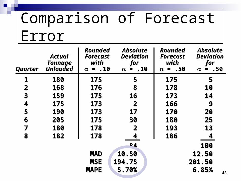
Comparison of Forecast Error
RoundedRounded AbsoluteAbsolute RoundedRounded AbsoluteAbsoluteActualActual ForecastForecast DeviationDeviation ForecastForecast DeviationDeviation
TonnageTonnage withwith forfor withwith forforQuarterQuarter UnloadedUnloaded = .10 = .10 = .10 = .10 = .50 = .50 = .50 = .50
11 180180 175175 55 175175 5522 168168 176176 88 178178 101033 159159 175175 1616 173173 141444 175175 173173 22 166166 9955 190190 173173 1717 170170 202066 205205 175175 3030 180180 252577 180180 178178 22 193193 131388 182182 178178 44 186186 44
8484 100100MADMAD 10.5010.50 12.5012.50MSEMSE 194.75194.75 201.50201.50
MAPEMAPE 5.70%5.70% 6.85%6.85%
49
Overview of Quantitative Approaches
1. Naive approach
2. Moving averages
3. Exponential smoothing
4. Trend projection
5. Linear regression
Time-Series Time-Series ModelsModels
Associative Associative ModelModel

50
Trend Projections
Fitting a trend line to historical data points Fitting a trend line to historical data points to project into the medium-to-long-rangeto project into the medium-to-long-range
Linear trends can be found using the least Linear trends can be found using the least squares techniquesquares technique
y y = = a a + + bxbx^̂
where ywhere y= computed value of the = computed value of the variable to be predicted (dependent variable to be predicted (dependent variable)variable)aa= y-axis intercept= y-axis interceptbb= slope of the regression line= slope of the regression linexx= the independent variable (= the independent variable (in this in this case timecase time))
^̂
51
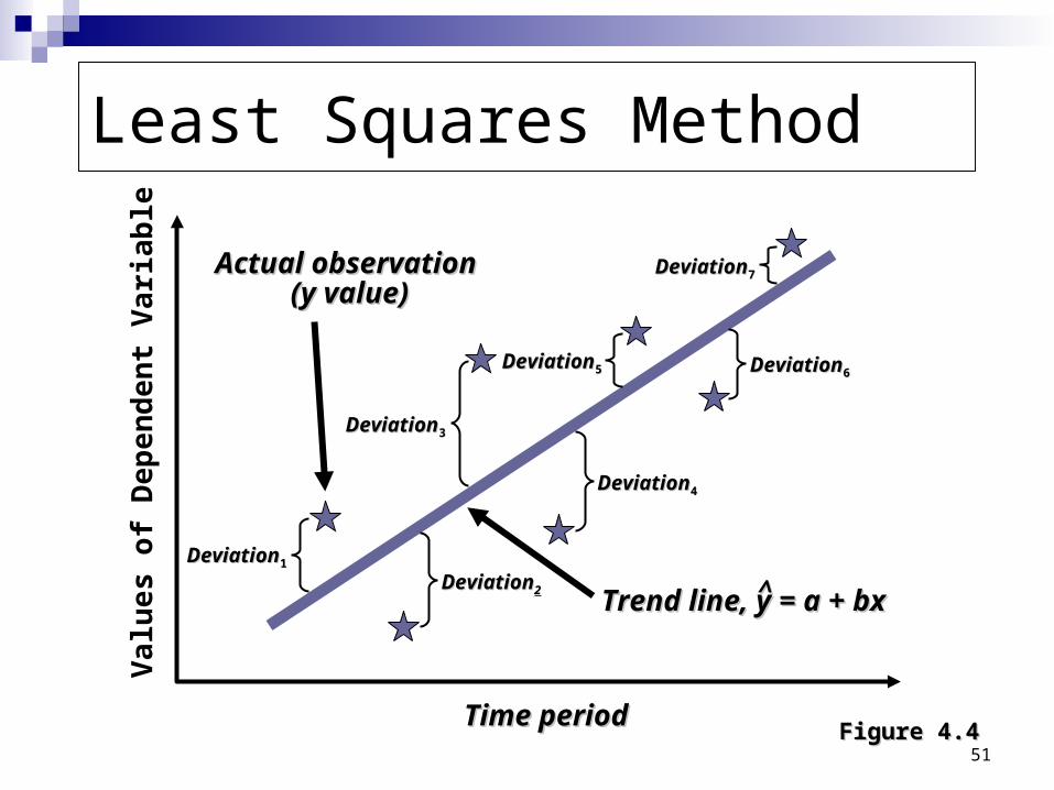
Least Squares Method
Time periodTime period
Va
lue
s o
f D
ep
end
en
t V
ari
able
Figure 4.4Figure 4.4
DeviationDeviation11
DeviationDeviation55
DeviationDeviation77
DeviationDeviation22
DeviationDeviation66
DeviationDeviation44
DeviationDeviation33
Actual observation Actual observation (y value)(y value)
Trend line, y = a + bxTrend line, y = a + bx^̂

52
Least Squares Method
Time periodTime period
Va
lue
s o
f D
ep
end
en
t V
ari
able
Figure 4.4Figure 4.4
DeviationDeviation11
DeviationDeviation55
DeviationDeviation77
DeviationDeviation22
DeviationDeviation66
DeviationDeviation44
DeviationDeviation33
Actual observation Actual observation (y value)(y value)
Trend line, y = a + bxTrend line, y = a + bx^̂
Least squares method minimizes the sum of the
squared errors (deviations)

53
Least Squares Method
Equations to calculate the regression variablesEquations to calculate the regression variables
b =b =xy - nxyxy - nxy
xx22 - nx - nx22
y y = = a a + + bxbx^̂
a = y - bxa = y - bx

54
Least Squares Example
b b = = = 10.54= = = 10.54∑∑xy - nxyxy - nxy
∑∑xx22 - nx - nx22
3,063 - (7)(4)(98.86)3,063 - (7)(4)(98.86)
140 - (7)(4140 - (7)(422))
aa = = yy - - bxbx = 98.86 - 10.54(4) = 56.70 = 98.86 - 10.54(4) = 56.70
TimeTime Electrical Power Electrical Power YearYear Period (x)Period (x) DemandDemand xx22 xyxy
19991999 11 7474 11 747420002000 22 7979 44 15815820012001 33 8080 99 24024020022002 44 9090 1616 36036020032003 55 105105 2525 52552520042004 66 142142 3636 85285220052005 77 122122 4949 854854
∑∑xx = 28 = 28 ∑∑yy = 692 = 692 ∑∑xx22 = 140 = 140 ∑∑xyxy = 3,063 = 3,063xx = 4 = 4 yy = 98.86 = 98.86

55
Least Squares Example
b b = = = 10.54= = = 10.54xy - nxyxy - nxy
xx22 - nx - nx22
3,063 - (7)(4)(98.86)3,063 - (7)(4)(98.86)
140 - (7)(4140 - (7)(422))
aa = = yy - - bxbx = 98.86 - 10.54(4) = 56.70 = 98.86 - 10.54(4) = 56.70
TimeTime Electrical Power Electrical Power YearYear Period (x)Period (x) DemandDemand xx22 xyxy
19991999 11 7474 11 747420002000 22 7979 44 15815820012001 33 8080 99 24024020022002 44 9090 1616 36036020032003 55 105105 2525 52552520042004 66 142142 3636 85285220052005 77 122122 4949 854854
xx = 28 = 28 yy = 692 = 692 xx22 = 140 = 140 xyxy = 3,063 = 3,063xx = 4 = 4 yy = 98.86 = 98.86
The trend line is
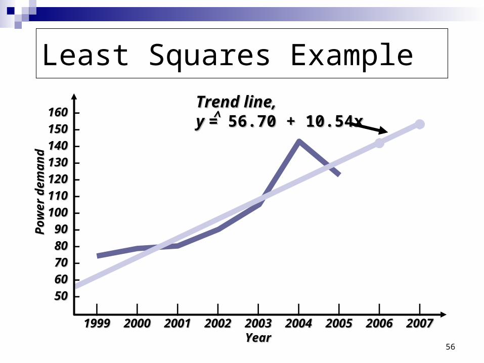
y = 56.70 + 10.54x^
56
Least Squares Example
| | | | | | | | |19991999 20002000 20012001 20022002 20032003 20042004 20052005 20062006 20072007
160 160 –
150 150 –
140 140 –
130 130 –
120 120 –
110 110 –
100 100 –
90 90 –
80 80 –
70 70 –
60 60 –
50 50 –
YearYear
Po
wer
dem
and
Po
wer
dem
and
Trend line,Trend line,y y = 56.70 + 10.54x= 56.70 + 10.54x^̂
58
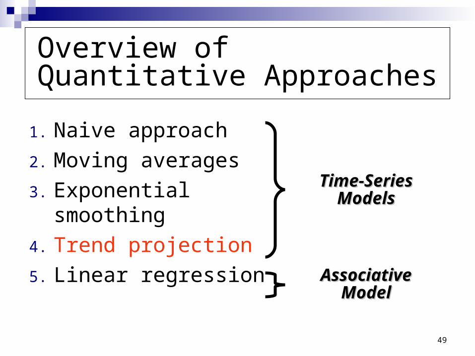
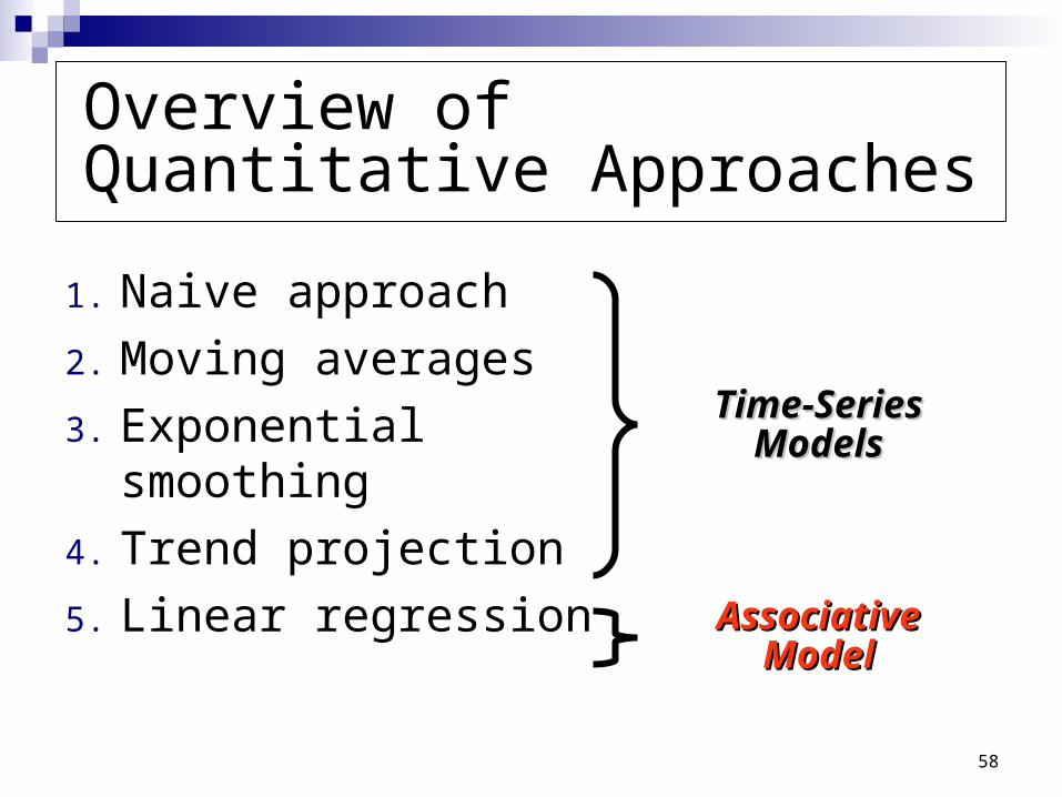
Overview of Quantitative Approaches
1. Naive approach
2. Moving averages
3. Exponential smoothing
4. Trend projection
5. Linear regression
Time-Series Time-Series ModelsModels
Associative Associative ModelModel
59
Associative Forecasting
Used when changes in one or more Used when changes in one or more independent variables can be used to predict independent variables can be used to predict
the changes in the dependent variablethe changes in the dependent variable
Most common technique is linear Most common technique is linear regression analysisregression analysis
We apply this technique just as we did We apply this technique just as we did in the time series examplein the time series example

60
linear regression analysis
Forecasting an outcome based on predictor Forecasting an outcome based on predictor variables using the least squares techniquevariables using the least squares technique
y y = = a a + + bxbx^̂
where ywhere y= computed value of the = computed value of the variable to be predicted (dependent variable to be predicted (dependent variable)variable)aa= y-axis intercept= y-axis interceptbb= slope of the regression line= slope of the regression linexx= the independent variable though = the independent variable though to predict the value of the to predict the value of the dependent variabledependent variable
^̂

61
Associative Forecasting Example
SalesSales Local PayrollLocal Payroll($000,000), y($000,000), y ($000,000,000), x($000,000,000), x
2.02.0 113.03.0 332.52.5 442.02.0 222.02.0 113.53.5 77
4.0 –
3.0 –
2.0 –
1.0 –
| | | | | | |0 1 2 3 4 5 6 7
Sal
es
Area payroll

62
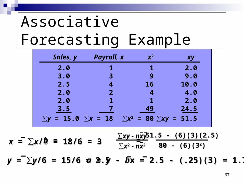
Associative Forecasting Example
Sales, y Payroll, x x2 xy
2.0 1 1 2.03.0 3 9 9.02.5 4 16 10.02.0 2 4 4.02.0 1 1 2.03.5 7 49 24.5
∑y = 15.0 ∑x = 18 ∑x2 = 80 ∑xy = 51.5
xx = = ∑∑xx/6 = 18/6 = 3/6 = 18/6 = 3
yy = = ∑∑yy/6 = 15/6 = 2.5/6 = 15/6 = 2.5
bb = = = .25 = = = .25∑∑xy - nxyxy - nxy
∑∑xx22 - nx - nx22
51.5 - (6)(3)(2.5)51.5 - (6)(3)(2.5)
80 - (6)(380 - (6)(322))
aa = = yy - - bbx = 2.5 - (.25)(3) = 1.75x = 2.5 - (.25)(3) = 1.75
63
Associative Forecasting Example
4.0 –
3.0 –
2.0 –
1.0 –
| | | | | | |0 1 2 3 4 5 6 7
Sal
es
Area payroll
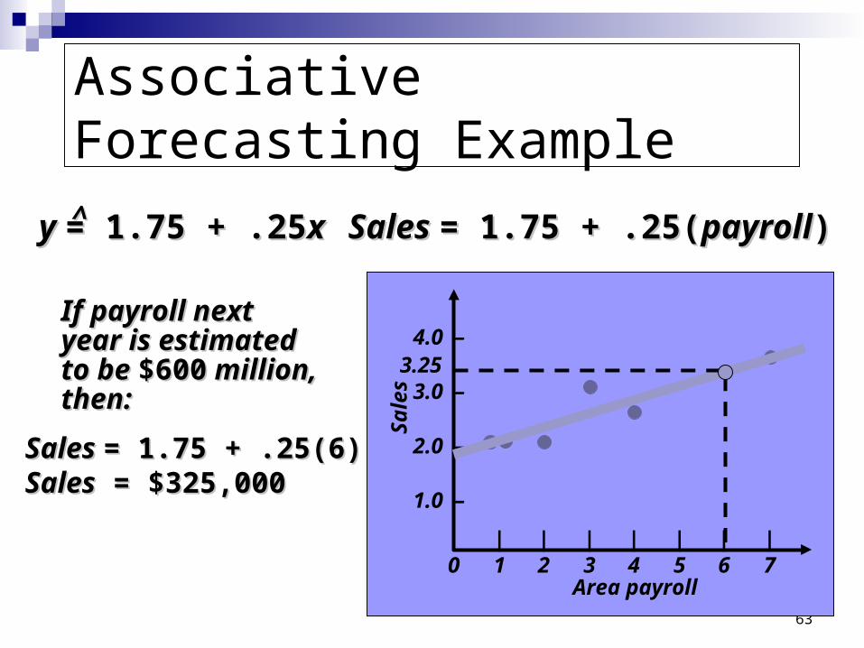
y y = 1.75 + .25= 1.75 + .25xx^̂ Sales Sales = 1.75 + .25(= 1.75 + .25(payrollpayroll))
If payroll next year If payroll next year is estimated to be is estimated to be $600$600 million, then: million, then:
Sales Sales = 1.75 + .25(6)= 1.75 + .25(6)SalesSales = $325,000 = $325,000
3.25
64
To measure the accuracy of the regression estimates, we must compute the standard error of the estimate, Sy,x.Sy,x.
This computation is called the standard deviation of the regression. It measures the error from the dependent variable y, to the regression line, rather than to the mean.
Standard Error of the Estimate
65
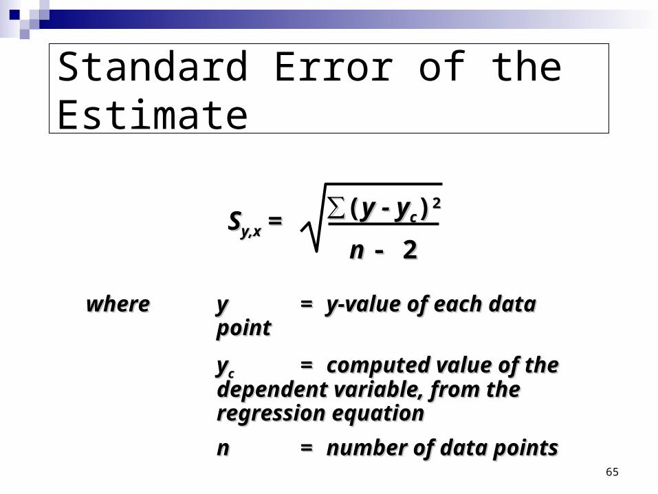
Standard Error of the Estimate
wherewhere yy == y-value of each data y-value of each data pointpoint
yycc == computed value of the computed value of the dependent variable, from the dependent variable, from the regression equationregression equation
nn == number of data pointsnumber of data points
SSy,xy,x = =∑∑((y - yy - ycc))22
n n - 2- 2

66
Standard Error of the Estimate
Computationally, this equation is Computationally, this equation is considerably easier to useconsiderably easier to use
We use the standard error to set up We use the standard error to set up prediction intervals around the prediction intervals around the
point estimatepoint estimate
SSy,xy,x = =∑∑yy22 - a - a∑∑y - by - b∑∑xyxy
n n - 2- 2
67
Associative Forecasting Example
Sales, y Payroll, x x2 xy
2.0 1 1 2.03.0 3 9 9.02.5 4 16 10.02.0 2 4 4.02.0 1 1 2.03.5 7 49 24.5
∑y = 15.0 ∑x = 18 ∑x2 = 80 ∑xy = 51.5
xx = = ∑∑xx/6 = 18/6 = 3/6 = 18/6 = 3
yy = = ∑∑yy/6 = 15/6 = 2.5/6 = 15/6 = 2.5
bb = = = .25 = = = .25∑∑xy - nxyxy - nxy
∑∑xx22 - nx - nx22
51.5 - (6)(3)(2.5)51.5 - (6)(3)(2.5)
80 - (6)(380 - (6)(322))
aa = = yy - - bbx = 2.5 - (.25)(3) = 1.75x = 2.5 - (.25)(3) = 1.75

68
Standard Error of the Estimate
4.0 –
3.0 –
2.0 –
1.0 –
| | | | | | |0 1 2 3 4 5 6 7
Sal
es
Area payroll
3.25
SSy,xy,x = = = =∑∑yy22 - a - a∑∑y - by - b∑∑xyxyn n - 2- 2
39.5 - 1.75(15) - .25(51.5)39.5 - 1.75(15) - .25(51.5)6 - 26 - 2
SSy,xy,x = = .306.306
The standard error The standard error of the estimate is of the estimate is $30,600$30,600 in sales in sales
69
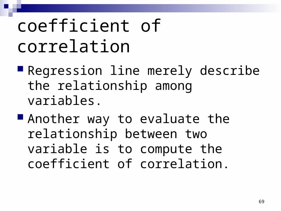
coefficient of correlation
Regression line merely describe the relationship among variables.
Another way to evaluate the relationship between two variable is to compute the coefficient of correlation.

70
How strong is the linear relationship between the variables?
Correlation does not necessarily imply causality!
Coefficient of correlation, r, measures degree of association Values range from -1 to +1
Correlation

71
Correlation Coefficient
r = r = nnxyxy - - xxy y
[[nnxx22 - ( - (xx))22][][nnyy22 - ( - (yy))22]]
72
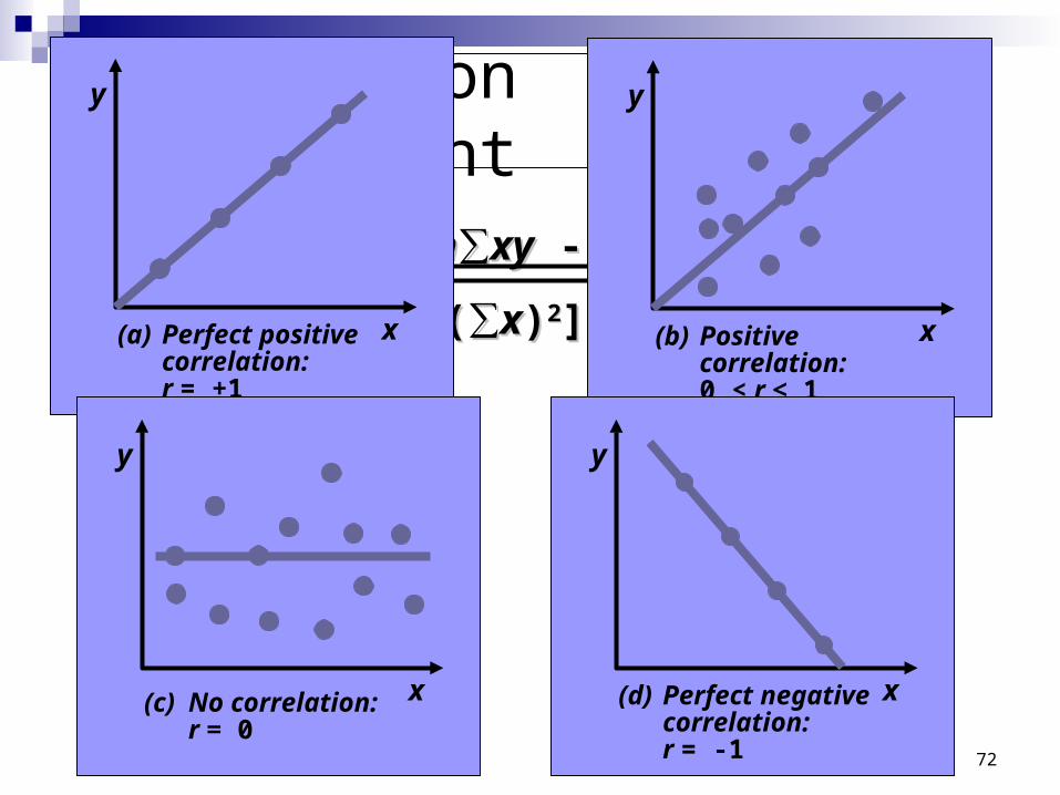
Correlation Coefficient
r = r = nn∑∑xyxy - - ∑∑xx∑∑y y
[[nn∑∑xx22 - ( - (∑∑xx))22][][nn∑∑yy22 - ( - (∑∑yy))22]]
y
x(a) Perfect positive correlation: r = +1
y
x(b) Positive correlation: 0 < r < 1
y
x(c) No correlation: r = 0
y
x(d) Perfect negative correlation: r = -1

73
Coefficient of Determination, r2, measures the percent of change in y predicted by the change in x Values range from 0 to 1 Easy to interpret
Correlation
For the Nodel Construction example:For the Nodel Construction example:
r r = .901= .901
rr22 = .81 = .81

74
Multiple Regression Analysis
If more than one independent variable is to be If more than one independent variable is to be used in the model, linear regression can be used in the model, linear regression can be
extended to multiple regression to extended to multiple regression to accommodate several independent variablesaccommodate several independent variables
y y = = a a + + bb11xx11 + b + b22xx22 … …^̂
Computationally, this is quite Computationally, this is quite complex and generally done on the complex and generally done on the
computercomputer

75
Multiple Regression Analysis
y y = 1.80 + .30= 1.80 + .30xx11 - 5.0 - 5.0xx22^̂
In the Nodel example, including interest rates in In the Nodel example, including interest rates in the model gives the new equation:the model gives the new equation:
An improved correlation coefficient of r An improved correlation coefficient of r = .96= .96 means this model does a better job of predicting means this model does a better job of predicting the change in construction salesthe change in construction sales
Sales Sales = 1.80 + .30(6) - 5.0(.12) = 3.00= 1.80 + .30(6) - 5.0(.12) = 3.00Sales Sales = $300,000= $300,000

76
Have nice day!