Some Approaches for Assessing Sustainability of Public Finances

Master’s thesis

Tuukka Sarvi

11.09.2011

Economics

Approved by the Head of the Economics Department xx.xx.20xx and awarded

the grade

_______________________________________________________

1. examiner 2.examiner

TIIVISTELMÄ

Tutkielmassa on oltava yhden sivun mittainen tiivistelmä (riviväli 1), joka

sijoitetaan ilman sivunumerointia

tutkielman alkuun ennen sisällysluetteloa. Tiivistelmä sisältää mm. seuraavat asiat

jäsennettynä omaan

tutkimukseen sopivalla tavalla:

o Tutkimuksen tavoitteet

o Tutkimuksen toteutustapa, menetelmät ja aineistot

o Tutkimuksen tulokset

o Avainsanat

ABSTRACT Tutkielmassa on oltava yhden sivun mittainen tiivistelmä (riviväli 1), joka

sijoitetaan ilman sivunumerointia

tutkielman alkuun ennen sisällysluetteloa. Tiivistelmä sisältää mm. seuraavat asiat

jäsennettynä omaan

tutkimukseen sopivalla tavalla:

o Tutkimuksen tavoitteet

o Tutkimuksen toteutustapa, menetelmät ja aineistot

o Tutkimuksen tulokset

o Avainsanat

Key words: public finance, fiscal sustainability, public debt sustainability, policy analysis

CONTENTS

1. Introduction ....................................................................................................................................... 2

1.1 Background and motivation ................................................................................................. 2

1.2 Objectives and limitations of the thesis ........................................................................... 3

1.3 Central definitions .................................................................................................................... 3

1.4 Structure of the thesis ............................................................................................................. 4

2. Challenges to sustainability ......................................................................................................... 4

2.1 The debt burden at a glance ................................................................................................. 4

2.1 Demographic transition ......................................................................................................... 6

2.2 Some sustainability estimates ............................................................................................. 8

3. Public sector balance sheet and income statement .......................................................... 10

3.1 Public sector balance sheet ................................................................................................. 11

3.2 Public sector income statement ........................................................................................ 12

4. Theoretical criteria for public finance sustainability ...................................................... 13

4.1 Inter-temporal budget constraint .................................................................................... 13

4.2 Model-Based Sustainability by Bohn (2005) ............................................................... 17

4.3 Convergence of the debt to output ratio ........................................................................ 17

4.4 Other criteria ............................................................................................................................ 18

5. Summary indicators of public finance sustainability ...................................................... 19

5.1 Finite horizon tax gap indicator ........................................................................................ 20

5.2 Infinite horizon tax gap indicator ..................................................................................... 21

5.3 Financing gap ........................................................................................................................... 22

5.4 Primary gap ............................................................................................................................... 22

5.5 Notes about the summary indicators .............................................................................. 23

6. Econometric tests of public finance sustainability ........................................................... 25

6.1 Unit root and cointegration tests of sustainability .................................................... 25

6.2 Model-based sustainability by Bohn (1998, 2005) ................................................... 27

6.3 Notes about econometric tests for sustainability ...................................................... 28

7. Value-at-Risk measure of sustainability ............................................................................... 28

8. Fiscal limits, fiscal space and sustainability ........................................................................ 32

8.1 Fiscal limits by Bi (2010) and others .............................................................................. 32

8.2 Fiscal space by Ostry et al. (2010) ................................................................................... 34

9. General equilibrium models ...................................................................................................... 38

9.1 GE-OLG model by Moraga and Vidal (2004) ................................................................ 38

9.2 Application of AGE-OLG model by van Ewijk et al. (2006) ..................................... 39

9.3 Application of CGE-OLG model by Andersen and Pedersen (2006) ................... 40

10. Generational accounting and sustainability ..................................................................... 42

11. Summary of strengths and weaknesses of the approaches ........................................ 47

12. Conclusion ...................................................................................................................................... 51

Bibliography ......................................................................................................................................... 53

Appendix 1: time series analysis .................................................................................................. 56

2

1. INTRODUCTION

1.1 BACKGROUND AND MOTIVATION

At the moment sustainability of public finances is a salient topic in many advanced economies.

Questions have been raised by various commentators, investors and analysts whether public

finances in the EU countries and in the US are on a sustainable track. After the financial crisis

of 2008-2009, the public debt of many countries has been on a steep upward trajectory due to

implementation of various stimulus and relief packages directed to financial sector and the

economy as a whole. A rising debt combined with long-term issues like the demographic

change which affects the balance between number of people in the labour force and number

of retirees, have alerted fiscal authorities to study the problem in detail. In fact, some

European countries like Greece, Ireland, Portugal, Spain and Italy are currently in serious

trouble with their public finances which is reflected in the high yield demanded from the

government bonds of these countries. As of this moment, Greece, Ireland and Portugal have

already received aid from other member states. It has been argued that the underlying

problem in Europe is the fragility of banks and the financial sector, not the public sector itself.

From the perspective of public finance sustainability this is not a valid point since problems of

any sector, like the financial sector, become problems of the public sector once they get big

enough.

Study of public finances is not important only in the current situation in US and in the EU. It

has been continuously pertinent issue in less developed countries. In less developed

countries, the public sector is usually more fragile and prone to shocks than in developed

countries. This is because the public sector of these economies is more vulnerable to exchange

rate fluctuations, commodity price fluctuations (like the price of oil), changes in interest rate

on government debt, sprees of high inflation and political turmoil. In the past, many emerging

market economies have experienced crises that have been closely tied to problems in public

finances. Some of these crises have led to debt restructuring efforts led by the IMF and some

have led to outright default.

The knowledge whether public finances are on a sustainable track is important in many

respects. Fiscal authorities of a country want to keep finances sustainable in order to give a

healthy ground for economic growth in the country. If public finances are not sustainable, this

affects the economy as a whole. This is evidenced by the fact that public sector accounts for a

3

large part of the economy in most countries. Furthermore, it is the public sector that provides

the institutions and services which are prerequisite for the normal function of corporations.

Thus, in order to avoid any crises in the public sector and the economy at large, it is valuable

for fiscal authorities to monitor the sustainability of public finances and inform politicians of

any significant developments in that area.

Also, the creditors of the government bodies follow the sustainability of public finances

closely. After all, their goal is to make profit and therefore they don’t want to pay too much for

government bonds. In order to have idea of the risk premium they require for the bonds, these

creditors, which are usually big banks, have to analyse the risks present in the public sector.

Therefore, the study of sustainability of public finances is crucial for them.

1.2 OBJECTIVES AND LIMITATIONS OF THE THESIS

First goal of this thesis is to critically examine various theoretical criteria that have been

proposed for sustainability in the literature. Second goal is to study and go through different

approaches which have been employed to measure the sustainability of public finances. The

study doesn’t attempt to be comprehensive: not all approaches to evaluate public finance

sustainability found in the literature are covered. Third goal is to analyse the strengths and

weaknesses of these approaches and compare them with one another. The method of study is

literature review.

1.3 CENTRAL DEFINITIONS

In this paper, a broad definition of public sector is used. It is defined to comprise of central

government, local governments, public corporations, central bank and social security funds.

The general definition of sustainability of public finances in this paper is the following: public

finances are sustainable if consolidated public sector is solvent given current policies. That is,

public sector is able to honour all its obligations (outlays, transfers, debt service, etc.) now

and in the future without adjusting its policies (tax rate, promised expenditures, etc.). This

concept is synonymous with fiscal sustainability and the two are used interchangeably. This

general definition elaborated later in Chapter 4 when various theoretical criteria of

sustainability are examined. Models and approaches to assess public finance sustainability

often use slightly different definitions for sustainability. However, the intent behind these

definitions is the same and it is described by the general definition given above.

4

1.4 STRUCTURE OF THE THESIS

The structure of the thesis is the following. First, in the second chapter, challenges to public

finance sustainability are outlined in the light of the existing debt burdens and large projected

costs due to the period of rapid demographic change many advanced economies are entering.

In the third chapter, public sector balance sheet and income statement are defined and

described. In the fourth chapter, several alternative theoretical criteria for sustainability are

examined. In the fifth chapter, summary indicators, the first approach to assess sustainability,

are examined. In the sixth chapter, econometric tests of fiscal sustainability are studied.

Seventh chapter defines and analyses a Value-at-Risk measure for sustainability. Eighth

chapter introduces the concepts of fiscal limit and fiscal space and their relation to

sustainability. In the ninth chapter, some general equilibrium models intended for analysis of

sustainability are examined. Tenth chapter defines and analyses generational accounting

approach to public finance sustainability. Eleventh chapter compares different approaches

presented and examines their strengths and weaknesses. The last chapter concludes.

2. CHALLENGES TO SUSTAINABILITY

Public finance sustainability is a timely topic for two main reasons. Firstly, in the aftermath of

the financial crisis of 2008-2009 public debt of many countries has rocketed to levels that

have never been seen before. Markets recognize this and require higher yields to compensate

for the additional risk. This has resulted in sovereign credit crises, especially in Europe.

Secondly, the long-run sustainability of public finances in many advanced economies is

threatened by the impeding large-scale demographic change. In the coming 50 years,

population ageing is projected to lead to significant increases in public expenditures due to

higher pension payments and health care costs. Furthermore, the demographic change leads

to lower expectations of economic growth because of reduced growth of the workforce. This

chapter offers a glance at the debt burden faced in economies around the world, describes the

extent of the coming demographic transition in advanced economies and records some

estimates of the long-run sustainability of public finances prepared by various governmental

institutions.

2.1 THE DEBT BURDEN AT A GLANCE

5

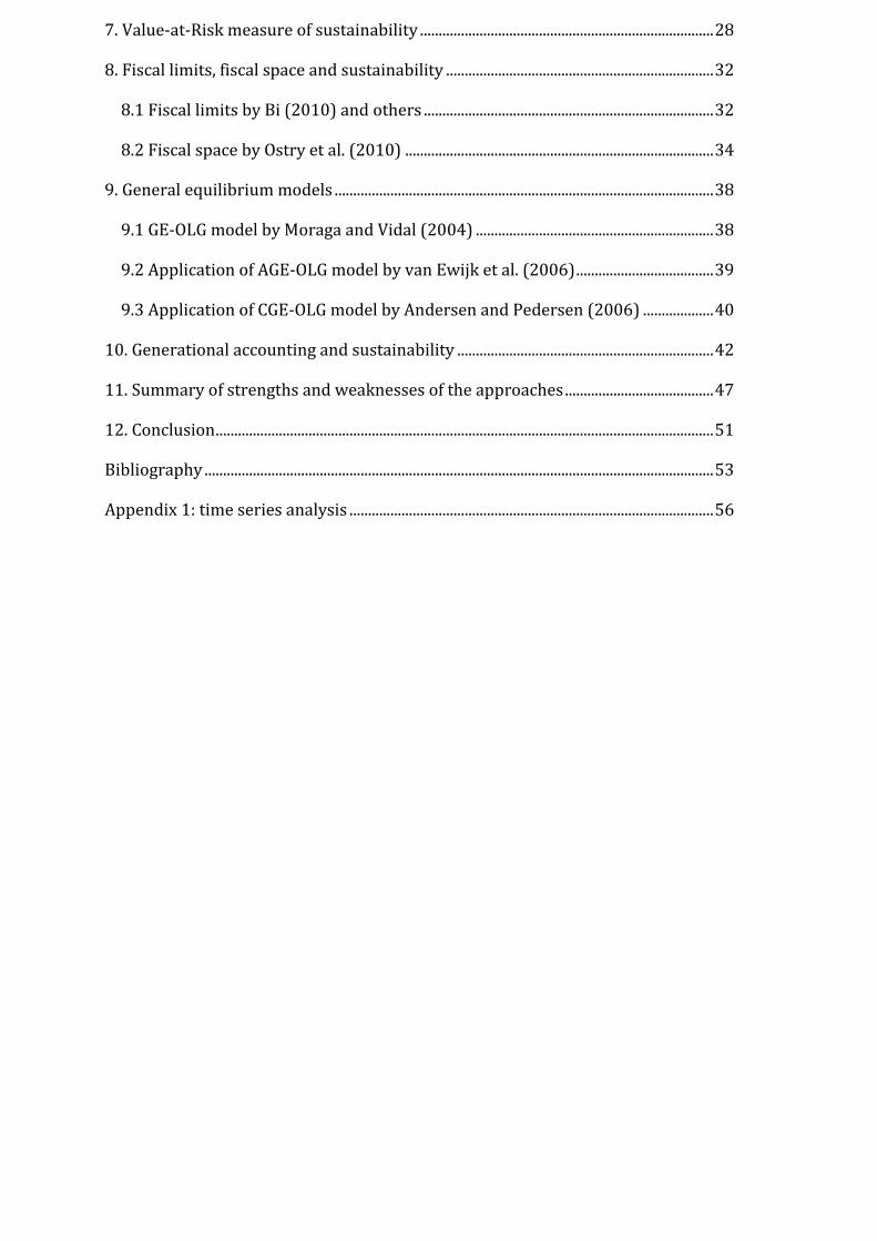
The extent of the debt burden varies greatly internationally. Some countries have little debt

while others have clearly too much for them to bear. Using gross debt per GDP as the

benchmark for indebtedness, it is seen that many advanced economies have significant stocks

of public debt while big emerging economies like China and Russia do not have much debt.

Figure 1 shows IMF estimates of general government gross debt per GDP in selected

economies in 2011.

Japan is projected to have the largest debt burden by a wide margin. Greece and Italy have

debt levels above 100 % of GDP. Greece is nearly in default and markets are suspicious of

Italy’s ability to pay back its loans which is reflected in recent hikes of bond yields. Despite its

massive debt stock Japan is not facing a credit crisis mainly because a large portion of the

public debt is held by Japanese citizens. While United States and big European economies

have taken a lot of new debt during recent years, they are still below the 100 % of GDP

boundary.

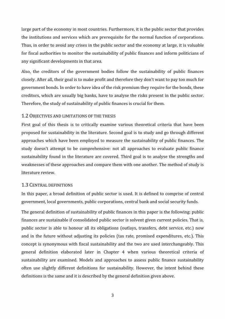
Figure 2 below shows the IMF 2011 estimates of net interest expense (interest expense minus

interest revenue) relative to general government revenues in the same set of countries as in

Figure 1 with the exception that China and India are missing due to data unavailability. Net

8,5

17,1

24,1

37,3

50,8

63,9

65,7

68,2

80,1

83

84,2

87,6

99,5

120,3

152,3

229,1

0 50 100 150 200 250

Russia

China

Australia

Sweden

Finland

Spain

Brazil

India

Germany

United Kingdom

Canada

France

United States

Italy

Greece

Japan

debt/GDP (%)

Figure 1. General government gross debt as percentage of GDP in 2011. Source: IMF World Economic Outlook estimates (April 2011).

6

interest expense per revenue measures the proportion of yearly revenues that governments

have to utilise just to pay the interest on existing debt.

It seems that in general, those countries that have big gross debt relative to GDP (Figure 1)

also spend large amount of their revenues on interest expenses. However, there are also

significant differences between the stories told by Figures 1 and 2 because what matters for

net interest payments is net debt, not gross debt. Furthermore, some countries have larger

revenue incomes relative to GDP and therefore spend for a given debt-to-GDP ratio spend less

interest expenses relative to revenues. Also, interest rates for different countries differ. In

Figure 2, Japan, which holds the largest stock of gross debt relative to GDP in the world,

doesn’t seem to especially burdened by interest payments. This is because according to IMF

statistics net debt in Japan is about half of the gross debt. Secondly, Japan faces very low

interest rates currently. IMF projects Finland and Sweden having net interest revenue in

2011. This results from the fact that net debt in Finland and Sweden is negative (stock of

assets is greater than stock of debt) because IMF calculations of net debt count pension funds

as government assets. Brazil is projected to have a large interest expense burden probably

because the it has to higher interest rates than many advanced economies.

2.1 DEMOGRAPHIC TRANSITION

1,8

1,3

-1,9

-1,1

4,5

14,9

4,8

8,2

1,1

5,1

5,8

9,9

15,1

4,5

-2,0 0,0 2,0 4,0 6,0 8,0 10,0 12,0 14,0 16,0

Russia

Australia

Sweden

Finland

Spain

Brazil

Germany

United Kingdom

Canada

France

United States

Italy

Greece

Japan

net intererest expense / revenue (%)

Figure 2. Net interest expense per general government revenue in 2011. Source: : IMF World Economic Outlook estimates (April 2011).

7

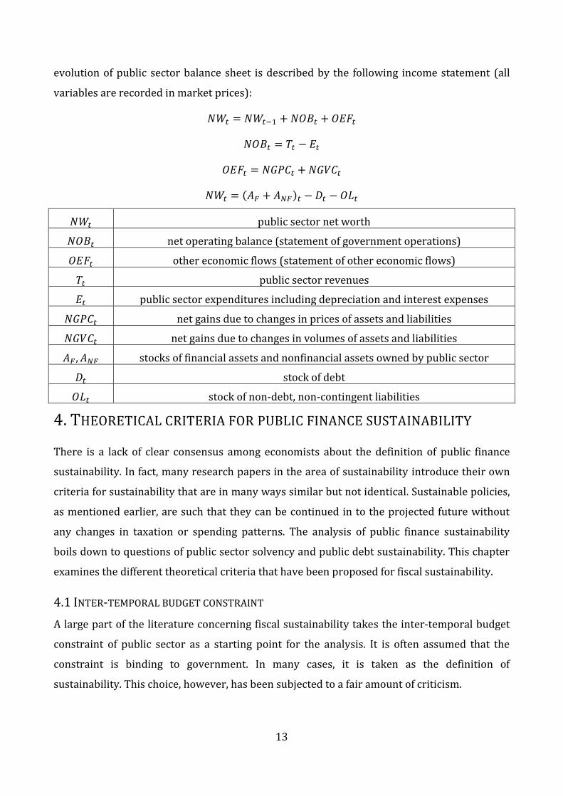
Major demographic changes are unfolding in the coming decades at the global level. Fertility

has been declining and longevity has been and is expected to keep increasing primarily due to

drop in the mortality rates at higher ages. Projections indicate that world total population will

keep on increasing and the population age composition will change significantly. At the global

level population is getting older. As a result of this, there is an upward trend in the

dependency1, although there is variation in the trend in different regions. Figure 3 shows the

projected trajectory of old-age dependency ratio in developed countries, less developed

countries and least developed countries.

The message of the figure is clear: during the next 50 years, the proportion of elderly in the

population of developed countries will approximately double.

The two main drivers behind the trend shown in Figure 3 are decrease in fertility and increase

in longevity. Fertility has been decreasing after peaking in the middle of the 20th century.

Currently, it has converged to a level of about 2 children per woman. Most of the developed

countries are now at the point when the large generations reach retirement age and new

comparatively smaller generations enter the job market which increases the dependency

ratio. Longevity has been on an increasing trend since 1950 with gains in life expectancy

amounting to 0.1 to 0.2 years per year. The continuing upward trend in longevity increases

1 Dependency measures the number of people outside work force relative to number of people in work force.

0

5

10

15

20

25

30

35

40

45

50

1950 1960 1970 1980 1990 2000 2010 2020 2030 2040 2050 2060

(%)

Figure 3. Old-age dependecy ratio ratio. The old-age dependency ratio is the ratio of the population aged 65 years or over to the population aged 15-64. Source: United

Nations, 2010 revision of World Population Prospects.

More developed countries

Less developed countries

least developed countries

8

the old-age dependency ratio because people spend longer times in retirement and thus the

age cohort 65+ increases in size. (United Nations 2011).

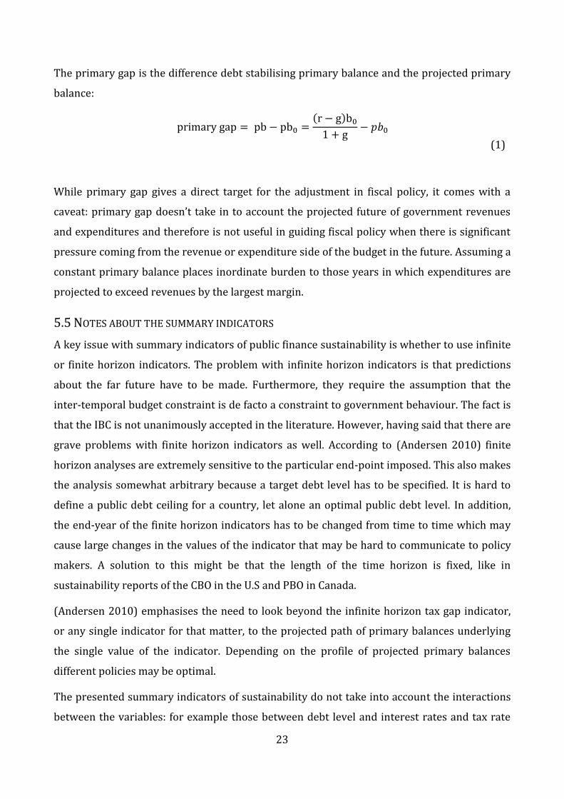
2.2 SOME SUSTAINABILITY ESTIMATES

The demographic change leads to increases in age-related public expenditures such as

pensions and health care in advanced economies. Many research institutes and governing

bodies such as the IMF, the European Commission and national governments have made

estimates of public finance sustainability that take in to account both the debt burden and the

projected long-run developments.

According to (European Commission 2009) age-related public expenditure is projected to rise

on average 4.3 percentage points of GDP by 2060 in the EU. The change is mainly due to

increases in pension, healthcare and long-term care spending. European commission assesses

the long-run sustainability of public finances by calculating so-called sustainability gaps.

These gaps measure the required adjustment by a shift in the projected path of primary

balances2. The size of the adjustment is such that the long-run solvency of the government is

re-established. Figure 4 shows the S2 sustainability gaps calculated by the European

Commission in 20093.

2 Primary balance equals government revenues minus expenditures excluding interest expenditure.

3 The S2 and other similar indicators are mathematically derived later in chapter 5 “Summary indicators of sustainability”.

9

The S2 sustainability gap for the EU as a whole was 6.5 % of GDP. This means EU countries

should immediately raise their tax ratios (tax income divided by GDP) by 6.5 % percentage

points in order to become solvent and be make fiscal policy sustainable. Alternatively, the

sustainability gap could be closed by making an expenditure cut of the same magnitude.

According to (European Commission 2009) about half of the gaps are due to the initial

budgetary positions (too much debt compared to projected primary surpluses) and half are

due to spending pressures arising from long-term demographic changes. There is significant

variation in degrees of sustainability problems in different EU countries. The gaps as

measured by S2 and S1 indicators range between -0.2% (Denmark) and 15% (Ireland). It is

notable that almost all countries have a positive sustainability gap as measured by both

indicators – this reflects the weak fiscal position due to economic crisis and the intensive

phase of demographic transition that most countries are entering. Most countries have gaps

near the EU average of 6.5 %.

In the United States, the Congressional Budget Office prepares long-term fiscal projections

and estimates of fiscal sustainability. These projections are made under two scenarios of

which the alternative scenario is perhaps the more realistic one. under two scenarios: the

extended-baseline scenario and alternative scenario. The alternative fiscal scenario extends

15

14,1

12,4

11,8

6,9

6,5

5,6

5,5

4,2

4

1,8

1,4

-0,2

-1 0 1 2 3 4 5 6 7 8 9 10 11 12 13 14 15 16

Ireland

Greece

United Kingdom

Spain

Netherlands

EU 27 average

France

Portugal

Germany

Finland

Sweden

Italy

Denmark

% of GDP Figure 4. S2 sustainability gap in selected European countries in 2009. Source: European

Commission 2009.

10

Congressional Budget Office’s 10 year baseline estimate further in time incorporating several

changes to the current law that are widely expected to occur or which alter some provisions

which be might be hard to sustain in the long run. CBO projects that the ageing of the

population and the rising cost of health care will cause spending on major mandatory health

care programs (Medicaid and Medicare) and Social Security to grow roughly by 12 % of GDP

by 2060 under the alternative fiscal scenario respectively. CBO uses fiscal gap indicators to

measure long-term sustainability of fiscal policies4. Under the alternative fiscal scenario the

gaps were 4.8 %, 6.9 % and 8.7 % for time horizons of 25, 50 and 75 years. (Congressional

Budget Office 2010).

In Canada, Office of the Parliamentary Budget Officer prepares long-term fiscal sustainability

estimates. Like in the U.S, two scenarios are used: a baseline scenario and an alternative

scenario. The difference between the two is that under the alternative scenario healthcare

costs are projected to keep growing at a high rate whereas in baseline scenario the growth is

assumed to be much more moderate. Due to population ageing, spending pressures in health

care and elderly benefits are projected to intensify. Under the alternative scenario, Canada

Health Transfer program, the largest health care –related expenditure of Government of

Canada, is projected to grow by about 3.5 % per GDP by 2060. Elderly benefits are estimated

to grow roughly by 1.2 % of GDP by 2060. PBO estimates fiscal gaps that are identical to those

estimated by CBO in the U.S. Under the alternative scenario fiscal gaps were 0.74 %, 1.38 %

and 1.89 % of GDP for time horizons 25, 50 and 75 years. (Parliamentary Budget Officer

2010).

3. PUBLIC SECTOR BALANCE SHEET AND INCOME STATEMENT

In the study of the sustainability of a country’s public finances it is important to consider the

public sector assets, liabilities, revenues and expenditures as comprehensively as possible.

Traditionally researchers have focused mainly on flow variables that appear in the budget

such as tax revenues, revenues from natural resources, government consumption and transfer

payments. In the past years, however, more attention has been devoted to the analysis of

stocks of assets and liabilities that constitute the government or public sector balance sheet.

4 Fiscal gap measure used by CBO is similar to S2 gap used by the European Commission. It is defined as the one-time permanent adjustment to primary balance per GDP (tax ratio or spending ratio or both) in order to stabilize debt-to-GDP ratio to its initial level in the end of the forecast horizon. For details see Chapter 5.

11

It has been recognized that changes in values of these assets and liabilities are and have been

an important factor affecting sustainability.

In this thesis, as all-encompassing as possible definition of public sector is used: public sector

consists of a central government, local governments, public corporations, a central bank and

social security funds. Basically all entities whose assets or liabilities can become government

assets should be included in the balance sheet analysis. Explicit and implicit guarantees and

contingent liabilities that affect government net worth (difference between value of assets

and liabilities) can have important implications for sustainability. Examples of these “hidden

debts” are unfunded social security programs, deposit insurance schemes and implicit bail out

guarantees to e.g. the financial sector.

This chapter goes through detailed versions of the public sector balance sheet and income

statement (or equivalently, budget constraint). The goal is to give the reader a broad

perspective of the factors that may affect public sector net worth.

3.1 PUBLIC SECTOR BALANCE SHEET

The 2001 IMF GFS Manual (International Monetary Fund 2001) sets out detailed definitions

for concepts and guidelines for accounting of public sector transactions and assets and

liabilities. In other words, it gives guidelines for implementation of the public sector balance

sheet. The 2001 IMF GFS Manual defines public sector net worth as the difference between

assets and liabilities at market prices. Both financial and nonfinancial assets and liabilities are

included. Changes in net worth could occur as a result of (1) budgetary transactions like tax

collection, grants and asset returns or government expenditures, interest expenses, payment

of subsidies and depreciation; (2) price effects, i.e. changes in the value of assets or liabilities;

and (3) changes in the volumes of assets and liabilities other than those resulting from normal

transactions, e.g. natural resource discoveries and disasters like floods and earthquakes which

can destroy assets.

An alternative definition of the public sector balance sheet is presented in (Easterly and

Yuravlivker 2000). It is broadly in line with the definition of 2001 IMF GFS Manual except in

that contingent contracts and value of the social security system is recorded directly in the

balance sheet. In 2001 IMF GFS Manual they are recorded as memorandum items outside

balance sheet. The public sector balance sheet and its constituents are presented in Figure 1.

12

In this view of the public sector balance sheet, government’s (= public sector) net worth is

analogous to book value of equity in balance sheets of private corporations.

FIGURE 5. PUBLIC SECTOR BALANCE SHEET AND ITS CONSTITUENTS.

Budgetary flows like tax revenues and government expenditures do not enter the balance

sheet but affect its evolution in time in a similar way as net sales and production costs affect

balance sheets of private corporations. Naturally, the future public sector revenues and

expenditures affect sustainability considerations significantly. Having said that, here the

expected present values of those flows do not enter the public sector balance sheet. The

balance sheet is consolidated from entities constituting the public sector so that liabilities

between these entities are disregarded and duplicate accounts are merged.

3.2 PUBLIC SECTOR INCOME STATEMENT

Public sector’s income statement accounts for the various flows that affect the evolution of its

balance sheet. IMF GFSM 2001 divides income statement in to two parts: statement of

government operations and statement of other economic flows. The former includes normal

budgetary items like revenues and expenses and net acquisition of financial and nonfinancial

assets and the net incurrence of debt. The latter records changes in public sector net worth

that are not a result of government transactions. These are changes in values and volumes of

assets and liabilities. Here these two statements are merged to yield an income statement

comparable to those of private corporations similarly as in (Costa and Juan-Ramón 2006). The

13

evolution of public sector balance sheet is described by the following income statement (all

variables are recorded in market prices):

( )

public sector net worth

net operating balance (statement of government operations)

other economic flows (statement of other economic flows)

public sector revenues

public sector expenditures including depreciation and interest expenses

net gains due to changes in prices of assets and liabilities

net gains due to changes in volumes of assets and liabilities

stocks of financial assets and nonfinancial assets owned by public sector

stock of debt

stock of non-debt, non-contingent liabilities

4. THEORETICAL CRITERIA FOR PUBLIC FINANCE SUSTAINABILITY

There is a lack of clear consensus among economists about the definition of public finance

sustainability. In fact, many research papers in the area of sustainability introduce their own

criteria for sustainability that are in many ways similar but not identical. Sustainable policies,

as mentioned earlier, are such that they can be continued in to the projected future without

any changes in taxation or spending patterns. The analysis of public finance sustainability

boils down to questions of public sector solvency and public debt sustainability. This chapter

examines the different theoretical criteria that have been proposed for fiscal sustainability.

4.1 INTER-TEMPORAL BUDGET CONSTRAINT

A large part of the literature concerning fiscal sustainability takes the inter-temporal budget

constraint of public sector as a starting point for the analysis. It is often assumed that the

constraint is binding to government. In many cases, it is taken as the definition of

sustainability. This choice, however, has been subjected to a fair amount of criticism.

14

The derivation of the inter-temporal budget constraint (IBC) starts with simple version of

public sector income statement, that is, one-period budget constraint which describes the

evolution of net debt:

( )

, where is the stock of public sector net debt, is the interest rate5, is the primary

balance of the public sector which equals revenues minus expenditures excluding interest

expenditure.

Solving the budget constraint recursively forwards in time gives:

( ) ( )

( ) ( ) ( )

…

( ) ∑( )

Taking the limit as n tends to infinity:

( ) ∑( )

The crucial assumption behind the inter-temporal budget constraint is that the first term

giving the present value of the government debt in infinity is assumed to be zero:

( )

This assumption is called the transversality condition (TC) or no-Ponzi-game condition (NPG).

By substituting it to the above equation, the inter-temporal budget constraint is received:

∑( )

The transversaility condition and inter-temporal budget constraint are equivalent in this

context. The inter-temporal budget constraint tells that the present value of the flow of

5 Here, constant interest rate is assumed for simplicity. Similar results can be derived in the case of time-dependent interest rate.

15

primary balances must equal the present stock of net debt. That is, government’s total net

liability must be equal to its total assets (flow of primary balances).

The transversality condition is sometimes called the no-Ponzi-game condition meaning that

government is not allowed to run a Ponzi game and that government doesn’t finance Ponzi

games. A Ponzi game or scheme is a system in which return to the principal of previous

investors is paid by new investments by subsequent investors. In the case of debt, the debtor

is running a Ponzi-game at the expense of the creditors when she always pays the interest by

issuing more debt.

Inter-temporal budget constraint is often analysed in the context of per GDP measures. The

underlying assumption is that GDP grows at a constant exponential rate6 so that

( ) . Substituting this gives:

( ) ∑( )

( ) ( )

∑

( ) ( )

(

)

∑(

)

, where lower-case symbols refer to the per GDP versions of net debt and primary balance.

Now there is a new variable to be considered in the analysis of sustainability: the growth rate

of GDP g. Taking limits as n tends to infinity:

(

)

∑(

)

The new version of the transversality condition states that

(

)

This is equivalent with the earlier transversality condition. For per GDP variables the

interpretation is just different: at the limit debt per GDP must grow at a gross rate slower than

6 Similar results can be derived in the case of time dependent growth rates.

16

.

/. For r>g, this allows exponentially growing debt per GDP trajectories. For r=g, debt per

GDP must be constant. For r<g, debt per GDP must converge to zero in an exponential rate.

The corresponding inter-temporal budget constraint is:

∑(

)

As noted earlier, there is disagreement among economists of whether IBC is a binding

constraint for governments.

(O’Connell and Zeldes 1988) show that Ponzi-games do not exist or equivalently the IBC must

hold in a credit market with a finite number of rational non-satiable participants over time.

This means that for IBC not to constrain government lending, the economy must consist of an

infinite number of agents entering it over time. This seems plausible, given infinite time

horizon of the analysis. However, the government constantly violating the IBC must be

infinitely-lived as well which seems less plausible.

(Bagnai 2004) finds it unreasonable that the IBC allows for explosive trajectories of debt-to-

gdp ratio. He argues that the IBC is not a fact of nature but rather it is a constraint imposed on

the behaviour of debtors by the rational creditors in a well-defined class of inter-temporal

equilibrium models. Therefore, he argues, if the class of models to which IBC is based is true,

“unsustainable” debt paths will never be observed. This is because the IBC must be respected

in these models in equilibrium and thus, observed violations of the constraint must be

temporary and hence irrelevant as far as the infinite-horizon asymptotic IBC is concerned.

Thus, IBC may appear to be violated only because 1) it is not binding in the economy for some

2) it is a temporary violation. Furthermore, (Bagnai 2004) seems to argue that assessment of

IBC in economies in which it is binding is a futile exercise: the possible violations are only

temporary and thus don’t require any actions. However, we would argue that examining

whether IBC holds or how big adjustment is required for it to hold in the projected future is

useful in these economies precisely because governments position as a debtor is grounded on

the fact that IBC holds: hence, fiscal authorities need to periodically adjust policies so that

creditors can reasonably expect IBC to hold.

There are several theoretical models in which IBC doesn’t have to hold. (Diamond 1965)

overlapping generations model may generate competitive equilibria in which growth rate of

17

the labour force exceeds the long-run return on capital. In these cases the economy is said to

be dynamically inefficient and government debt can increase at rate higher than the interest

rate violating the IBC. Counter-argument to this is that empirical evidence indicates that most

of the advanced economies are dynamically efficient (Abel et al. 1989). However, (Croix and

Michel 2002, 192) show that in an overlapping generations model based on (Diamond 1965)

IBC doesn’t have to hold given that government can tax both the young and the old generation

even if the economy is dynamically efficient. Other examples of where IBC doesn’t constraint

government in dynamically efficient economy are (Persson 1985) and (Wigger 2009).

4.2 MODEL-BASED SUSTAINABILITY BY BOHN (2005)

(Bohn 2005) criticizes the use of IBC in sustainability analyses and introduces criterion for

sustainability which he terms Model-Based Sustainability (MBS). The MBS criterion

generalises the traditional deterministic IBC to a world with uncertainty. Bohn argues that the

question which policies are sustainable is a general equilibrium question about the behaviour

of potential government creditors. Different assumptions about the behaviour of creditors

lead to different conclusions about sustainability of fiscal policies. Under the assumptions that

potential creditors are infinitely-lived optimizing agents, government doesn’t run a negative

debt in the long-run and that financial markets are complete (Bohn 2005) argues that the

inter-temporal budget constraint takes the form (Model-Based Sustainability criterion)

∑ , -

, where is the economy’s pricing kernel for contingent claims on period (t+n) (the state-

contingent discount factor). The MBS criterion is derived from optimizing creditor behavior. It

differs from the usual IBC in that the discount rates for future surpluses depend on the

distribution of primary surpluses across states of nature. (Bohn 2005) shows that the above

IBC condition can lead to government facing constraints other than the traditional IBC.

4.3 CONVERGENCE OF THE DEBT TO OUTPUT RATIO

A common criterion for fiscal sustainability is the convergence of the debt-to-GDP ratio to a

finite value (the boundedness criterion):

18

This condition was first proposed as a sufficient condition for sustainability in (Domar 1944).

A stricter form of this criterion is that debt-to-output ratio must eventually converge back to

its initial value. It is analysed for example in (Blanchard et al. 1990).

The above condition requires that eventually debt cannot grow at a rate greater than growth

rate g of the economy. Inter-temporal budget constraint and the transversality condition

requires that debt cannot grow at a rate greater than the interest rate r. Thus, when r > g, as is

usually assumed, this criterion is stricter than the inter-temporal budget constraint. When r <

g, the situation is the opposite.

The asymptotic boundedness condition of debt to output ratio compares the governments

collateral, fraction of output taxed, to the stock of debt. It can be argued that the boundedness

condition is always a looser condition that the inter-temporal budget constraint. It is

reasonable to assume that primary balance cannot exceed output in any period. Thus,

assuming IBC holds implies

∑(

)

∑(

)

for all t, assuming r>g. Therefore, if r>g, the assumption that primary balance can never

exceed output requires the boundedness of debt-to-output ratio for all t. This means that the

boundedness criterion is looser also when r>g.

4.4 OTHER CRITERIA

(Roubini 2001) argues that the inter-temporal budget constraint is too loose criterion for

fiscal sustainability. According to the inter-temporal budget constraint a government could

run very large primary deficits for a long time provided that it could commit to run primary

surpluses in the long run to satisfy the IBC. Roubini argues that this is not realistic for three

reasons. Firstly, government cannot credibly commit to such a path. Secondly, adjustment

required to run large enough primary surpluses in the long run would be highly costly and

inefficient given distortionary taxation – i.e. it doesn’t make sense to have marginal tax rates

of 70 % in the long run to compensate for low marginal tax rates of 10 % in the short run.

Thirdly, if the adjustment falls on government consumption rather than taxes it may again be

unfair and inefficient to cut government spending and services to low levels in the long run to

allow large spending in the short run. (Roubini 2001) suggest that a very practical criterion

for sustainability: public debt can be viewed as sustainable as long as the public debt to GDP

19

ratio is non-increasing. This means that primary balance to output ratio should fulfil the

following condition:

(Artis and Marcellino 2000) distinguish between solvency and sustainability. They define that

a government is solvent if the IBC is fulfilled, that is, governement is capable during an infinite

horizon to service its debt. On the other hand, according Artis and Marcellino sustainability is

a more imprecise concept referring ability of government under current policies to achieve a

pre-specified debt ratio in a finite time horizon.

The Treaty of Maastricht sets explicit conditions for fiscal sustainability of the EMU countries.

Article 109 (1) of the treaty requires “sustainability of the governments financial position” for

a country’s eligibility to EMU. The treaty further defines the criteria to assess the

sustainability by setting ceiling values of 3 % and 60 % for deficit and debt to GDP ratios

respectively. The issue of sustainability is also elaborated in The Stability and Growth Pact by

introducing the medium target of a fiscal position close to balance or in surplus thus

tightening the deficit rule of the Treaty of Maastricht. It is unclear what “a position of close to

balance or surplus in medium term” actually constitutes. In the EU framework sustainability is

thus defined as non-violation of predefined conditions which include an arbitrary debt to

output ceiling which is consistent with the boundedness criterion of sustainability.

5. SUMMARY INDICATORS OF PUBLIC FINANCE SUSTAINABILITY

After discussing the theoretical criteria for sustainability it is now possible to turn to the

different approaches employed in sustainability assessments. Firstly, summary indicators

which employ rather simple discounted cash flow calculations are studied.

Summary indicators are perhaps the most common approach to analyse sustainability in

practice. These indicators are derived from the government budget constraint governing the

evolution of debt as a function of interest rates, growth rate of the economy and future

primary balances. These derivations do not use an explicit economic model to account to for

the various interactions between the model variables and hence the indicators derived can

only be regarded as giving an approximation of the degree of sustainability. They take as an

input the projected primary balances, interest rates and growth rates of the economy. The

20

indicators are widely used by for example European commission, national governments and

the International monetary fund to assess sustainability.

5.1 FINITE HORIZON TAX GAP INDICATOR

The derivation is based on the equation describing the evolution of net debt per output that

was derived earlier:

(

)

∑(

)

Compounding the equation to period t+n gives

(

)

∑(

)

Defining a specific time horizon (t, T) and a debt-to-output target level to be achieved at the

end of the time horizon gives the condition for permanent constant adjustment to primary

balance relative to output required to achieve the target:

(

)

∑(

)

( )

Using the formula for geometric series gives the size of the gap:

( . /

∑ . /

) ( )

( . /

) ( )

This indicator is equivalent to the S1 indicator used by the European commission. In S1

indicator the end of the time horizon is the year 2060 and the target debt-to-output ratio is 60

%. Congressional Budget Office in the US and Office of the Parliamentary Budget Officer in

Canada use the same type of indicator which they term fiscal gap. They use time horizons of

25, 50 and 75 years. They require that at the end of time horizon debt-to-output ratio returns

to its initial value.

Finite horizon tax gap indicator determines a target level for debt-per-GDP ratio to be reached

at the end of the specified time horizon. It is called tax gap indicator because the adjustment is

measured in terms of change in primary balance to output ratio so that the indicator gives the

21

permanent change required in the total tax ratio, total tax revenues per GDP, to reach the

target debt-per-GDP ratio at the end of the time horizon. For example, if FTGAP = 3 %, this

means a permanent raise of 3 % in the tax income per GDP ratio would close the sustainability

gap if the tax hike didn’t have any dynamic effects. However, the required permanent

adjustment in the primary balances per output can be realised equally well by cutting

expenditures relative to GDP or by any combination of tax revenue increase and expenditure

cut that permanently increase primary balance relative to output by the amount specified by

the indicator.

Finite horizon tax gap indicator (and any other tax gap indicator for that matter) divides the

burden of adjustment equally (as a proportion of GDP) to the years belonging to the time

horizon. This means that the change in net taxes paid relative to total output is equal in every

period. Thus, the finite horizon tax gap indicator assumes that the required adjustment is

smoothed over the time horizon.

5.2 INFINITE HORIZON TAX GAP INDICATOR

The infinite horizon tax gap indicator is based on the inter-temporal budget constraint. It

measures the permanent constant adjustment to primary balance to output ratio required to

satisfy the IBC:

∑(

)

( )

( ) ( ∑ . /

)

The sustainability indicator S2 used for example by the European commission is equivalent to

the above indicator. Assuming r > g, infinite horizon tax gap can be derived from the formula

of finite horizon tax gap by taking the limit T tends to infinity. This just means that if debt

converges to a finite level at infinity it is consistent with IBC when r>g.

ITGAP indicator divides the required adjustment relative to GDP evenly to infinite time

horizon. Similarly as the finite horizon indicator, ITGAP is a tax gap indicator which means

that its value can be interpreted as immediate permanent change to tax ratio required for IBC

to hold. The change to primary balances can come equally well from expenditure cuts.

22

5.3 FINANCING GAP

The needed adjustment as measured by finite or infinite horizon tax gaps can be divided to

the time horizon in ways other than smoothing the adjustment evenly as a percentage of GDP.

Financing gap takes the flow of predicted future primary balances and compares it with the

current level of net debt. In the case of infinite horizon, it gives the immediate adjustment to

the debt per GDP level needed to satisfy the inter-temporal budget constraint:

∑(

)

The indicator measures the adjustment required in present value terms relative to output

unlike tax gaps in which the adjustment was given in a form of an annuity. Measuring the gap

in present value terms might be useful in some cases. At minimum, it is a good way to

demonstrate the extent of the sustainability problem. A similar indicator can be defined for

finite horizons. In that case, the financing gap measures the immediate required change in

debt per GDP level to attain the target level of debt per GDP at the end of the chosen time

horizon. Financing gap is analysed e.g. in (Giammarioli et al. 2007).

5.4 PRIMARY GAP

Unlike previous indicators, the primary gap assumes the constancy of primary balances in the

future. It determines the constant primary balance that would satisfy the required infinite or

finite horizon sustainability conditions. In the infinite horizon case, primary gap indicator is

defined as the difference between the required constant primary balance to satisfy the

government’s inter-temporal budget constraint and the projected primary balance. It was

proposed by (Buiter, Persson, and Minford 1985). Assuming r>g and substituting to

the IBC and solving for gives:

( )

This is called the “debt stabilising primary balance”. It means that if , debt ratio

decreases and if , debt ratio increases. The only stable long-run steady state is

because other values of primary balance lead either to unbounded increase or

decrease of the debt-to-output ratio. The condition is equivalent with the criterion of

sustainability proposed by (Roubini 2001) which requires the debt-to-output ratio to be non-

increasing.

23

The primary gap is the difference debt stabilising primary balance and the projected primary

balance:

( )

(1)

While primary gap gives a direct target for the adjustment in fiscal policy, it comes with a

caveat: primary gap doesn’t take in to account the projected future of government revenues

and expenditures and therefore is not useful in guiding fiscal policy when there is significant

pressure coming from the revenue or expenditure side of the budget in the future. Assuming a

constant primary balance places inordinate burden to those years in which expenditures are

projected to exceed revenues by the largest margin.

5.5 NOTES ABOUT THE SUMMARY INDICATORS

A key issue with summary indicators of public finance sustainability is whether to use infinite

or finite horizon indicators. The problem with infinite horizon indicators is that predictions

about the far future have to be made. Furthermore, they require the assumption that the

inter-temporal budget constraint is de facto a constraint to government behaviour. The fact is

that the IBC is not unanimously accepted in the literature. However, having said that there are

grave problems with finite horizon indicators as well. According to (Andersen 2010) finite

horizon analyses are extremely sensitive to the particular end-point imposed. This also makes

the analysis somewhat arbitrary because a target debt level has to be specified. It is hard to

define a public debt ceiling for a country, let alone an optimal public debt level. In addition,

the end-year of the finite horizon indicators has to be changed from time to time which may

cause large changes in the values of the indicator that may be hard to communicate to policy

makers. A solution to this might be that the length of the time horizon is fixed, like in

sustainability reports of the CBO in the U.S and PBO in Canada.

(Andersen 2010) emphasises the need to look beyond the infinite horizon tax gap indicator,

or any single indicator for that matter, to the projected path of primary balances underlying

the single value of the indicator. Depending on the profile of projected primary balances

different policies may be optimal.

The presented summary indicators of sustainability do not take into account the interactions

between the variables: for example those between debt level and interest rates and tax rate

24

and economic growth. Thus, the results can be taken only as an approximation of the extent of

the sustainability problem.

The values received from the sustainability indicators depend crucially on the inputs: flow of

predicted primary balances, current debt level, interest rates and growth rates. The values of

the inputs have to be determined by using some economic and econometric forecasting

models. Therefore, these models and their assumptions, whatever they may be, represent an

underlying framework behind any estimates of sustainability given by the summary

indicators. These underlying economic models are an essential factor behind the results.

Hence, the analysis of any values of the summary indicators of sustainability will be

incomplete without careful analysis of underlying economic forecasting models.

One problem with the summary indicators is that there is not any explicit consideration for

uncertainty of the estimated values of indicators. Many sustainability reports like (European

Commission 2009) include scenario and sensitivity analyses in which the various inputs to the

calculation of summary indicators, such as the interest rates and growth rates, are varied and

new values for the indicators are determined. These types of sensitivity analyses are essential

feature of the practical use of the indicators because in order to draw any policy implications,

it is important to get a sense of the uncertainty inherent in the point estimates of summary

indicators. However, it would be even better, if models (the underlying framework) that yield

the inputs to calculations and the indicators itself would explicitly account for uncertainty.

There have been some extensions to the presented indicators that account for uncertainty, e.g.

in (Giammarioli et al. 2007). Ideally, the result of sustainability analyses with uncertainty

would be a set of estimated distributions for the output variables like the sustainability gaps.

Policy implications of a sustainability gaps as measured by the summary indicators are not

straightforward. According to (Barro 1979) tax smoothing argument, tax rates should be kept

constant over time to minimize tax distortions, allowing government budget to absorb

variations in net expenditures. Hence, temporary expenditure variations would be absorbed

through budget, while permanent expenditure changes require a permanent change in the tax

rate. Thus, different underlying reasons causing the sustainability gaps may lead to different

conclusions about needed policy actions. For instance, in the case of demographic change due

to permanent lower level of fertility and permanent higher longevity which are the primary

causal factors behind the sustainability problems in developed countries, it would seem that

25

the correct policy response would be an immediate permanent change in the tax rate.

However, this argument disregards the issues of intergenerational equity.

6. ECONOMETRIC TESTS OF PUBLIC FINANCE SUSTAINABILITY

This section examines the various econometric tests that have been proposed as tests of fiscal

sustainability. In this strand of literature, different theoretical conditions for sustainability are

tested with historical data of, among other things, debt and deficits. This section is divided

into two parts: unit root and cointegration tests of sustainability and model-based

sustainability by (Bohn 1998; Bohn 2005). Definitions of central mathematical concepts used

in the chapter can be found in Appendix 1.

6.1 UNIT ROOT AND COINTEGRATION TESTS OF SUSTAINABILITY

One of the first attempts to test sustainability by econometric means is (Hamilton and Flavin

1986). In that paper, Hamilton and Flavin derive a statistical test to determine whether the

inter-temporal budget constraint or equivalent transversality condition holds in empirical

data. They use a detailed framework accounting for the general debt structure of government

bonds and possibility of deficit monetising (money printing). Their null hypothesis which is

equivalent with the IBC is the following:

∑( )

, where is the real market value of government debt, r is average real return earned on

government bonds, and is real primary balance: a sum of tax revenue and

seigniorage revenue minus government spending.

Specifically, they test whether in the formulation:

( ) ∑( )

, where is regression disturbance term and denotes the expectations of creditors which

Hamilton and Flavin assume to be formed rationally.

(Hamilton and Flavin 1986) find that the IBC holds (i.e. ) in the empirical data for US

during the years 1960-1984 and conclude that IBC seems to have been a restriction on

26

government borrowing during that period. It is noteworthy that (Hamilton and Flavin 1986)

test the whether IBC holds in the data but take no stance of whether it should hold. Thus, a

negative result wouldn’t have meant that government policy had not been sustainable but

rather that IBC has not been a relevant constraint for government during the period in

question.

(Wilcox 1989) uses the same data set as Hamilton and Flavin and finds that if the hypothesis

of constant interest rate is relaxed and stochastic violations to the inter-temporal budget

constraint are considered as well, then the null hypothesis that IBC holds in the data must be

rejected.

(Trehan and Walsh 1988) show that if real revenues, real spending and real debt have unit

roots, a stationary deficit (including interest payments) is sufficient to guarantee that IBC

holds. Trehan and Walsh test these statements in US data spanning years 1890-1986 and find

that it is consistent with IBC.

(Trehan and Walsh 1991) generalizes results of their previous paper. Firstly, with variable

discount rates, IBC holds if debt is difference-stationary and if the discount rate is strictly

positive. This statement can be understood by noting that if debt is difference-stationary

with mean the expected debt n-periods forward is:

, -

In other words, expected growth of debt is linear. This implies that the expected present

value of debt tends to zero in accordance with the transversality condition and the inter-

temporal budget constraint because discounting factor decays exponentially.

Secondly, (Trehan and Walsh 1991) show that IBC holds if a quasi-difference of debt

is stationary for some and if debt and primary surpluses are

cointegrated, covering the case of non-stationary with-interest deficits. The intuition behind

this condition is the fact that is stationary with implies that

asymptotic rate of growth of debt is which is in turn less than interest rate . Hence, the

asymptotic expected present value of debt tends to zero in line with the transversality

condition.

Using these tests described above, (Trehan and Walsh 1991) find that postwar US fiscal policy

is consistent with the IBC.

27

(Bohn 2005) applies unit root tests to a longer sample of US data spanning the time period

1792-2003. He finds that there is no credible evidence of unit roots in the U.S. debt-GDP and

deficit-GDP ratios and that (Trehan and Walsh 1988) condition for IBC to hold is satisfied in

the data. Absence of unit roots means that debt-GDP ratio is stationary and thus policies are

sustainable.

6.2 MODEL-BASED SUSTAINABILITY BY BOHN (1998, 2005)

(Bohn 1998) introduces an approach to sustainability testing which he names Model-Based

Sustainability (MBS). The condition for model-based sustainability which is a generalization of

the usual inter-temporal constraint was referred to earlier (MBS criterion):

∑ , -

Under the MBS framework sustainability analysis reduces to testing whether or not the

primary balance-output ratio responds positively to increases in public debt-output ratio. The

regression to test this is:

, where is a constant and is a composite of determinants of the primary balance other

than the initial stock of debt. (Bohn 1998) shows that if in the equation above, is

bounded as a share of GDP and if the present value of GDP is finite, then fiscal policy satisfies

the MBS criterion.

(Bohn 1998) estimates above regression for US data encompassing the period 1916-1995. He

finds strong evidence in favour of in US data for the period 1916-1995. (International

Monetary Fund 2003, 113-152) applies Bohn’s MBS test to a sample of industrial and

developing countries. The results signal that the sustainability condition holds for industrial

countries and developing countries with low debt ratios. It fails for developing countries with

high debt ratios. (Bohn 2005) continues in this track and finds robust positive response of

primary surpluses to fluctuations in the debt-GDP ratio in the US during the period 1792-

2003 and hence concludes that US fiscal policy has been sustainable. (Mendoza and Ostry

2008) use MBS test for 34 emerging market and 22 industrial countries over the period 1990-

2005. They find that the MBS condition for fiscal solvency is consistent with the data for both

emerging market and industrial countries.

28

While (Mendoza and Ostry 2008) consider MBS framework a powerful and tractable tool to

find out if government policies have been sustainable, they note two caveats with the

framework. Firstly, the test assumes complete markets. In the case of incomplete asset

markets where there are not sufficient state-contingent claims to fully hedge against possible

shocks, (Mendoza and Ostry 2008) argue that tighter debt limits than those imposed by the

MBS criterion are required. Secondly, they note that it is unclear how to interpret results

when is statistically insignificant or when . One interpretation is that failure of the test

indicates that MBS criterion is not a relevant constraint for government borrowing in the

economy. Alternatively, such a failure could mean that either MBS is a relevant constraint but

market anticipates a policy change or government policies are unsustainable.

6.3 NOTES ABOUT ECONOMETRIC TESTS FOR SUSTAINABILITY

Bohn’s model based sustainability approach to econometric testing seems robust and

preferable to the earlier unit root tests. However, the problem with traditional application of

econometric tests is that they provide information about the sustainability of past policies

only. This is fine if the purpose of the research is to examine sustainability in retrospect.

However, usually a more interesting question is the sustainability of the current fiscal policy

as projected in to the future. If econometric tests were applied to projected future data, they

could give information about the sustainability of current fiscal stance, that is, the expected

future fiscal policy. The usefulness of such an exercise is not clear, however, because the

researcher can build in any feedback relations in to the projected data. If projected data and

sustainability testing were done in credibly separate processes, and the projections were

trustworthy, applying econometric tests to the projected data might be useful. We were

unable to find any papers doing this.

7. VALUE-AT-RISK MEASURE OF SUSTAINABILITY

Every assessment of public finance sustainability contains considerable amount of

uncertainty because in order to assess sustainability uncertain predictions in to the far future

have to be made. This chapter goes through a Value-at-Risk framework of sustainability by

(Barnhill and Kopits 2003) which attempt explicitly to account for the uncertainty in

predictions of future values of relevant variables such as budget balances, growth rates and

interest rates.

29

In financial mathematics and risk management Value-at-Risk (VaR) is a commonly used risk

measure of the risk of loss on a portfolio of financial instruments. It measures the worst

possible loss over a target horizon with a given level of confidence. For example, if one-month

95 % Value-at-Risk for a portfolio of stocks is 1 million , this means that the monthly loss on

the portfolio is greater than or equal to 1 million with probability 5 %. VaR methodology is

commonly used in the financial industry to manage risk exposure.

(Barnhill and Kopits 2003) apply VaR methodology to analyse the public finance

sustainability. The approach simulates a distribution of possible future financial conditions

for the government and assesses the probability of financial failure given this distribution.

The analysis of Barnhill and Kopits is based on the income statement of the consolidated

public sector encompassing both monetary and fiscal authorities:

Public sector revenue consists of tax receipts less government transfers (T), determined by

the level of economic activity, the tax structure and administrative efficiency; net revenue

from resource sales (N), a function of production level, production cost and resource price;

and income from seigniorage (S). Expenditure is comprised of government consumption (G),

made up of mandatory and discretionary payments on wages, goods and services; and

interest payments given by the product of average interest rate (r) and the net stock of public

debt outstanding (B). The net debt consists of domestic liabilities less assets and of foreign

liabilities less assets. Also, the public sector may hold a stock of net unfunded contingent

liabilities (C) relating to social security programs, deposit insurance schemes, insurance for

natural disasters or other government guarantees that may realized and converted into B.

Realization of C is affected by the level of economic activity, demographic trends, effectiveness

of bank supervision, bank capitalization and occurrence of natural disasters.

In the framework, the net value of the public sector at t=0 is the sum of the present values of

the terms in the income statement7:

( ) ( )

∑( )

∑( )

∑( )

7 (Barnhill and Kopits 2003) use the term net worth instead of net value. Net value is used here because net worth has a different definition in this thesis.

30

, where Z’ is the primary balance generated by the existing fiscal system (tax structure and

mandatory spending programs in existence at t=0), is the probability of realizing

contingency at time t and is the discounted net amortization schedule of the net debt

so that ∑ ( ) . Calculation of the net value assumes that there is no

discretionary adjustment in tax structure or government spending in the future. Also, income

from seignorage is assumed to equal zero at all times.

If net value is non-negative, the public sector is deemed solvent and policies are sustainable8.

In traditional assessments of sustainability, the expected value of net value is studied. Here V

is explicitly recognized as a stochastic variable and its distribution estimated.

(Barnhill and Kopits 2003) model the public sector net value as a function of underlying risk

variables:

( )

The equation tells that the public sector net value depends on the present and future level of

output (q) , interest rates at home and abroad ( ), the exchange rate (f) world commodity

prices (p_N) and the domestic price level (p).

The risk variables determine the financial environment thus and the asset prices and present

values of future revenues and expenditures. Therefore, by simulating the risk variables,

distributions for government assets, liabilities and net value can be estimated. From the

estimated distributions, relevant Value-at-Risk measures can be calculated.

In order to simulate the behaviour of the risk variables, Barnhill and Kopits assume that they

follow known stochastic processes. Barnhill and Kopits use different stochastic processes for

description of different variables. For example, they use Brownian motion for rates of return,

output and prices and time-dependent mean reversion process for interest rates. Parameters

of the stochastic processes are estimated from historical data. By estimating the historical

correlations between the risk variables, they can reconstruct the correlation structure

inherent in the variables. In practice this means that imposing the correlation structure of the

risk variables on the error terms of the stochastic procesess. This way Barnill and Kopits can

combine the stochastic processes describing the time-evolution of the risk variables and the

correlation structure inherent in to yield simulated values of the risk variables.

8 The net value is related to inter-temporal budget constraint in the following way: . Having a positive net value is equivalent to saying that government doesn’t run a Ponzi scheme.

31

Barnhill and Kopits apply their Value-at-Risk framework to study the sustainability of public

sector finances in Ecuador. Based on data from year 2000 they simulate distribution of public

sector net value in year 2001. They estimate that one-year 95 % VaR of Ecuador was 29 US$

billion. Because, absent risk, net value of the public sector was 8 US$ billion, it is equivalent to

say that net value of the public sector with 5 % probability was -21 US$ billion. It is

noteworthy that assessment focused expected value of public sector would have found no

sustainability problem because expected public sector net value was 8 US$ billion.

Insolvency, that is negative net value of the public sector, is predicted to occur with 35 %

probability. Their simulations indicate that the principal sources of fiscal risk for Ecuador

were volatility in the interest yield spread, the exchange rate, and oil prices together with

their comovements.

The VaR approach of Barnhill and Kopits is a valuable tool for analysis of public finance

sustainability. It attempts to account for most of the complexities involved in the analysis of

sustainability. Specifically, it is an improvement to traditional approaches because uncertainty

is explicitly and more realistically modelled. In addition, a comprehensive view of the public

sector net value is undertaken with due recognition to the fact that changes in values of

government assets and liabilities significantly affect public sector solvency and policy

sustainability.

At heart of the VaR approach is the estimation of distribution of government net value and

thus solvency. Both effects from changes in asset values and present values of future

budgetary flows are accounted for. Usage of the VaR approach is not limited to calculation of

specific VaR estimates. Other risk measures such as conditional Value-at-Risk can be

calculated as easily. By estimating the distribution of government net value, the VaR approach

allows for the complete risk management of public sector assets and liabilities.

(Barnhill and Kopits 2003) note that the VaR approach is open to question on several

grounds. Firstly, the variances and covariances of the risk variables estimated from past data

may not provide a reliable picture of future risks. This shortcoming is mitigated by the fact

that VaR approach flexible is in that the risk models can be readjusted on the basis of expert

opinion. Secondly, Barnhill and Kopits point out that the contingent liability modelling is

lacking because risks stemming from e.g. financial system defaults are not accounted for in a

comprehensive manner. Thirdly, the approach needs quite rich data about public sector assets

32

and liabilities which is not available in every country. Public sector balance sheets are a

minimum input requirement for VaR analysis.

8. FISCAL LIMITS, FISCAL SPACE AND SUSTAINABILITY

Recently a few novel approaches have been developed for estimating public debt ceiling for a

country. Knowledge of an upper limit for a country’s public debt would be very useful for

sustainability assessments since it would give indication of how much more debt the country

is able to sustain at maximum. Here two approaches are analysed. The first tries to determine

so-called fiscal limit for a country. Fiscal limit is the point beyond which taxes and

government expenditures can no longer adjust to stabilize the value of government debt. This

approach stems from the literature on monetary and policy interactions and appears in for

example in (Bi 2010), (Cochrane 2010) and (Leeper and Walker 2011). The second approach

attempts to estimate a debt ceiling for a country based on the country’s past record of fiscal

policy. It is developed in (Ostry et al. 2010).

8.1 FISCAL LIMITS BY BI (2010) AND OTHERS

The concept of fiscal limits appears in novel and growing strand of literature on monetary and

fiscal policy interactions. Fiscal limit of a country means the point beyond which taxes and

government expenditures can no longer adjust to stabilize the value of government debt. In

other words, it is the maximum level of debt that can be accommodated by a government

solely by fiscal instruments. After an economy hits the fiscal limit, the government has to

stabilise debt by monetary policy: seigniorage revenue generates enough surplus to stabilise

the level of debt. Alternatively, if this kind of money printing is not possible, government can

default on some of its obligations such as the debt or promised expenditures. Thus,

determining the fiscal limit of a country and comparing it to the present and projected future

levels of debt gives indication of how much room the government has left for fiscal policy

adjustments. This, in turn, is valuable piece of information in public finance sustainability

assessments.

The most common economic rationale for existence of fiscal limits follows from the Laffer

curve. The Laffer curve depicts an inverse U-shaped between the tax rate and collected tax

revenue. Under distortionary taxation, higher tax levels lead to diminishing incentives to

work, save and invest and thus to lower levels of realised tax bases. As the tax rate is

33

increased, at some point the marginal relative decrease in the tax base will exceed the

marginal relative increase in tax rate and from that point on the collected tax revenue will fall.

Thus, there is some level of the tax rate which maximizes tax revenue. Given a level of

promised government expenditures, the existence of Laffer curve implies some maximum

stream of primary surpluses that the government can generate. Because government debt is

valuable only to the extent it is backed up by flow of future primary surpluses (assuming

seigniorage revenues are zero), and the present values of this flow is bounded, the size of

government debt relative to output must be bounded as well. Fiscal limit B* can be defined

(Bi 2010):

∑

( )

, where Q is the discount factor, is the maximum tax revenue and G is government

spending and transfers. The actual fiscal limit is usually below the economic fiscal limit

defined above because political considerations prevent tax rates reaching revenue maximising

levels.

The fiscal limit is a model-dependent measure like most of the measures related to

sustainability. Here we describe the way (Bi 2010) attempts to estimate the fiscal limit.

(Bi 2010) constructs an infinite-horizon model of a closed economy in which fiscal limits arise

endogenously from Laffer curves. The economy has a simple linear production technology and

productivity follows an exogenous stochastic process. Government is modelled as an

automaton which finances purchases and lump-sum transfers to households by collecting tax

revenue and issuing bonds. Purchases are modelled by an exogenous stochastic process and

transfers follow productivity counter-cyclically. Government follows a simple tax rule in

which tax rate rises linearly with increases in debt. (Bi 2010) models government default by

random draw from distribution of fiscal limit. If the current level of debt surpasses the draw,

government defaults on a fraction of its outstanding debt. If not, government fully honours all

its obligations. By modelling default by a random draw from the distribution of fiscal limit, (Bi

2010) abstracts from strategic concerns of default related to models of political economy.

In (Bi 2010), a representative household chooses consumption and leisure and government

bond purchases to maximize expected present value of utility. Proportional tax on labour

distorts household’s choice and induces a Laffer curve in the economy. The Laffer curve, given

34

level of government purchases and lump-sum transfers, results in a ceiling for surplus in any

period and gives rise to a fiscal limit. In (Bi 2010), fiscal limit is also affected by political

willingness to raise taxes near revenue maximising rates. This is modelled by the parameter

in the following expression for fiscal limit

∑

( )

, where is a discount factor depending on household’s subjective discount factor and

marginal utility of consumption when tax rate is set at the peak of the Laffer curve, is

political risk factor, is maximal revenue at time i and and are government transfers

and purchases respectively.

The distribution of the fiscal limit is country-specific and depends on underlying parameters

of the model. However, (Bi 2010) emphasises that the fiscal limit is independent of

equilibrium conditions of the model. (Bi 2010) estimates distribution of the fiscal limit by

using Markov Chain Monte Carlo simulation.

(Bi 2010) calibrates the model to economies of Canada, New Zealand, Belgium, Japan and

Sweden and observes that the model predicts distributions of fiscal limits consistent with the

sovereign credit ratings on these countries. The model also produces a nonlinear “S-shaped”

relationship between sovereign risk premia and the level of government debt which is

consistent with empirical evidence.

The model by (Bi 2010) is one attempt to estimate fiscal limits and endogenise the

relationship between interest rates on government debt and the debt level. Even though the

model is fairly simple it produces encouraging qualitative results that match empirical

observations. The model has many assumptions that are not very realistic such as the

simplistic logarithmic utility function and linear production function, assumption that

government is an automaton and the deterministic tax rule followed by government. In spite

of all this, our opinion is that (Bi 2010) and other recently published papers on fiscal limits

represent a new and promising way to look at public finance sustainability.

8.2 FISCAL SPACE BY OSTRY ET AL. (2010)

(Ostry et al. 2010) introduce another approach to estimate the degree to which a country has

room for fiscal manoeuvring, that is the fiscal space, by looking at the historical record of the

35

country’s fiscal policy. The intent of the approach is similar to that of fiscal limits though

methodology differs significantly. (Ostry et al. 2010) define fiscal space as the difference

between the current level of public debt and the debt limit implied by the country’s historical

record of fiscal adjustment. Their approach to estimating an upper limit for public debt is

based on the fiscal reaction function pioneered by (Bohn 1998) which determines country’s

primary balance as a function of the debt level.

First component of the analysis of (Ostry et al. 2010) involves determination of the fiscal

reaction function. Ostry et al. observe that governments usually behave responsibly

increasing primary surplus in response to rising debt service in order to stabilize the debt

ratio. However, this cannot always be true because at sufficiently high levels of debt this

would require primary balance to exceed GDP. They plot primary balance ratio against public

debt ratio for a sample 23 advanced economies over the period 1970-2007 and observe that

there seems to be a S-shape or loosely sigmoid-shape relationship between the two. In other

words, while fiscal effort is increasing in debt level, the effort eventually diminishes as tax

increases and spending cuts become less and less feasible politically. This relationship is

depicted by the solid line in Figure 2.

The second component of the analysis by Ostry et al. is the determination of the interest rate

schedule which gives the ratio of primary balance to GDP that leads to unchanged debt ratio

as a function of debt ratio. This is equivalent with the “debt-stabilising primary balance”

defined in chapter 5:

( ( ) )

( ( ) )

The dashed line in Figure 2 depicts the interest rate schedule. Given that interest rate

doesn’t depend on the debt level, which is the case for low levels of debt, the interest rate

schedule is a linear function of the debt level. However, as the debt level rises and country’s

solvency comes under question, creditors start to demand increased yields because of the

default risk. This means the interest rate schedule turns steeply upward at some point ( in

Figure 2).

36

FIGURE 6. DETERMINATION OF DEBT LIMIT. THE SOLID LINE DEPICTS THE FISCAL

REACTION FUNCTION AND THE DASHED LINE DEPICTS THE EFFECTIVE INTEREST RATE

SCHEDULE PB=(R-G)D. SOURCE: OSTRY ET AL. (2010).

Figure 2 presents a heuristic treatment of the determination of the debt limit according (Ostry

et al. 2010). The two curves, primary balance reaction function (solid line) and interest rate

schedule (dashed line), intersect at two points. The intersection at a lower level of debt ratio

corresponds to the conditionally stable long-run public debt ratio ( ). The intersection at a

higher level of debt ratio corresponds to the debt limit ( and ). Given that debt ratio is

below the debt limit, absent shocks, the country’s debt ratio will eventually converge to the

long-run stable ratio because below primary balance response is such that debt ratio

increases and above it is such that debt ratio decreases. Ostry et al. define two debt limits:

and . The former is based on the interest rate schedule which assumes that interest rate

doesn’t increase with the debt ratio. The latter is based on assumption that due to the

possibility of stochastic shocks to primary balance markets will require a risk premium on top

of the risk-free rate after some point which causes the interest rate schedule to turn

upwards and to intersect the primary balance reaction function earlier than in a riskless

world. Beyond the debt limit the country’s debt ratio will increase without bounds in absence

of historically extraordinary fiscal effort.

37

(Ostry et al. 2010) estimate fiscal reaction function relating primary balances to lagged debt

and various economic, structural and institutional variables, as well as country-specific fixed

effects using a sample of 23 advanced economies over the period 1970-2007. The function is

cubic in lagged debt allowing for two apparent inflection points in the fiscal reaction function.

Ostry et al. assume that coefficients of the debt ratio in this function are the same for all

countries. Varying fiscal reactions for different countries are allowed for by the country-

specific fixed effects other independent explanatory variables.

(Ostry et al. 2010) determine interest rate schedule using two techniques. Firstly, they use a

linear form of the interest rate schedule with either historical or projected interest rate-

growth rate differential. Secondly, they calculate the interest rate schedule endogenously by

using country-specific histories of shocks to primary balances. This second technique

accounts for the fact that interest rate rises as country gets nearer its debt limit.

Using the estimated fiscal reaction functions and interest rate schedules, (Ostry et al. 2010)

calculate values of long-run debt ratio ( ), debt limit ( ) and fiscal space (difference

between debt ratio projected for 2015 and the debt limit) for different advanced economies.

Furthermore, in order to take in to account the uncertainty, they report the estimates of fiscal

space in terms of probability that a country has a given amount (0, 50 or 100 % of GDP) of

remaining fiscal space. For example, they estimate the probability that a country has any fiscal

space left is 6.3 %, 34.4 %, 71.8 % and 96.2 % for Greece, Portugal, United States and Finland.

Their estimates of debt limits, fiscal spaces and the associated probabilities vary greatly

between the countries in the sample.

The approach to estimate debt limits and resulting fiscal space by (Ostry et al. 2010) appears

promising. The debt limit is calculated based on a country’s past record of fiscal policies. The

framework with fiscal reaction function and interest rate schedule is both simple and quite

easy to practically implement. The crucial interaction between the level of debt and interest

rates is explicitly modelled. Furthermore, the debt limit and fiscal space are pretty intuitive

concepts and thus can be relatively easily communicated. Weakness of the approach is that it

needs quite a lot of data for determination of the fiscal reaction function. Such data is not

usually available for countries for sufficiently broad range of debt ratio levels. For this reason

Ostry et al. had to assume common regression coefficients and use in part common data for

estimation of the reaction functions. In addition, the approach doesn’t look at the public sector

balance sheet as a whole: it doesn’t explicitly account for government assets, expected

38

spending pressures e.g. due to aging and contingent liabilities. It would be preferable to use

net worth or net debt to GDP ratios instead of gross debt to GDP ratio.

9. GENERAL EQUILIBRIUM MODELS

This section describes three papers that analyse public finance sustainability by using general

equilibrium models: GE-OLG model by (Moraga and Vidal 2004), application of AGE-OLG

model by (van Ewijk et al. 2006) and application of CGE-OLG model by (Andersen and

Pedersen 2006). Many papers that use general equilibrium models to study sustainability are

very theoretical. These three papers were chosen for further study because in them, these

models are applied for practical policy analysis.

9.1 GE-OLG MODEL BY MORAGA AND VIDAL (2004)

(Moraga and Vidal 2004) investigate fiscal sustainability in a general equilibrium overlapping

generations model with endogenous growth resulting from human capital formation through

educational spending. Interest rate and growth rate of the economy which have a crucial

effect on long-run sustainability are determined endogenously in the model. In the model

fiscal sustainability means that economic equilibrium exists in every period.

The model’s economy has three sectors: households, firms and the public sector. Household

sector consists of individuals that live through three periods: childhood, adulthood and old-

age. These individuals maximize utility which is derived from private and public consumption

in adulthood and old-age and their children’s expected wage level. Consumption, saving and

educational spending are financed by labour income which depends on individual’s human

capital. An individual’s human capital is determined in their childhood by her parents’ human

capital and educational spending. This process of human capital formation is the engine of

growth in the economy. Production occurs in firms which use physical and human capital as

inputs. Each period, firms choose demand for labour to maximize profits in a competitive

setting. The public sector consists of the government which levies taxes, pays pension benefits

to retirees, finances public consumption and reimburses existing stock of debt along with

interest payments.

(Moraga and Vidal 2004) derive a system of two differential equations which determine the

dynamics of the economy. They describe the evolution of stock physical capital and

government debt relative to stock of human capital. No general analytical solution exits for

39

the system. Moraga and Vidal calibrate the model roughly to European Union data. By means

of simulations they study the effect of a demographic shock which is projected to occur in the

EU during the next 50 years. They show that the demographic change leads to unsustainable

situation unless fiscal policies are changed in response. Proper fiscal rules guarantee

convergence to a new equilibrium and thus sustainability.

The strengths of the model by (Moraga and Vidal 2004) concerning sustainability assessments

lie on theoretical analysis of an economy. It allows for study of the impact of various shocks

and fiscal rules to sustainability. However, it is not so well suited to practical sustainability

assessments concerning actual countries. The overlapping generations framework only allows

for a crude description of the dynamics because length of the period is 1/3 of a lifetime, i.e.

very long (Moraga and Vidal use 30 years). Furthermore, it is hard to calibrate. To assess

sustainability more realistically, adjustments to the model such as shorter time period, more

detailed generational structure and richer description of the tax and pension policies are

needed.

9.2 APPLICATION OF AGE-OLG MODEL BY VAN EWIJK ET AL. (2006)

(van Ewijk et al. 2006) use a large scale applied general equilibrium model with overlapping

generations of households to study ageing and its effect on sustainability of public finances in

Netherlands. The model they use is called GAMMA and it is constructed for the purpose of

analysing long-term public policy issues.

The model consists of the following agents: households, government, firms, pension funds and

the foreign sector. Households are divided up into 100 age cohorts. Households decide on

labour supply and private saving, firms decide on demand for labour and capital and pension

funds decide on pension contributions and benefit levels. Agents are rational and forward-

looking and optimise in a consistent microeconomic framework. The model includes a

comprehensive set of generational accounts for all current and future generations. The Dutch

economy is modelled as a small open economy. Interest rate determined in world capital

markets and it is not affected by domestic policies. Domestic and foreign goods are assumed

to be perfect substitutes. Perfect labour and capital markets are assumed. Furthermore, the

model is deterministic.

(van Ewijk et al. 2006) construct a baseline projection which forecasts the evolution of public

finances and the economy under unchanged policies from year 2006 onwards. Detailed

40

demographic projections up to year 2100 are employed. In the baseline scenario, they assume

that age-specific expenditures increase at the rate of productivity of private sector

productivity and aggregate non-age-related expenditures increase at the rate of GDP growth.

They assume annual rate of labour-augmenting technological change of 1.7 %, average real

market rate of return of 3 % and inflation of 2 %. Government revenues are determined

endogenously from household and firm behaviour except for natural resource revenues which

are evolve in line with separate projections. Van Ewijk et al. also conduct sensitivity tests

around this baseline projection by varying parameter values and assumptions.

(van Ewijk et al. 2006) find that Dutch public finances are unsustainable in the long run. This

is primarily due to population ageing which leads to significant increases in pension and

health care expenditures and projected depletion of natural gas reserves and the associated

revenue flow. They estimate that total debt, the sum of net debt (official debt minus financial

assets of the government) and implicit debt that is due to projected deficits, is 2 times GDP in

2006. This indicator is equivalent with financing gap derived earlier in chapter 5. The annuity

value of this total debt amounts to 2.6 % GDP which is the sustainability gap equivalent with

infinite horizon sustainability gap. They conduct sensitivity tests around the baseline scenario

and estimate a confidence interval of (0.9%, 5.1%) for the sustainability gap.

The study by (van Ewijk et al. 2006) is a successful application of generational equilibrium

framework to assessment of public finance sustainability. Model is detailed and structurally

rich and therefore should be able to produce accurate projections concerning the Dutch

economy. Interactions between the various forces in the economy are better accounted for

than if separate models were used for projecting the inputs to sustainability calculations.

Weakness of this approach is that a lot of detailed data about the economy under analysis is

required. Secondly, a lot of effort needs to be put in to build such a large scale model. Finally,

despite the structural richness of the model, there is no practical guarantee about its

predictive accuracy.

9.3 APPLICATION OF CGE-OLG MODEL BY ANDERSEN AND PEDERSEN (2006)

(Andersen and Pedersen 2006) use a large scale dynamic computable general equilibrium

overlapping generations model to study the long-term sustainability of fiscal policies in

Denmark. The model they use is called DREAM, the Danish Rational Economic Agents Model,

41

developed for the specific purpose of evaluating medium- to long-term effects of fiscal policy

in Denmark.9

DREAM model represents a small open economy with a fixed exchange rate regime, perfect

mobility of capital and imperfect substitutability of Danish and foreign products in

consumption and production. The model uses a detailed household structure based on

projections of Danish population. The adult population has 85 generations and a

representative household is generated for each of the generations. Each household optimizes

its labour supply, consumption and savings decisions given perfect foresight. The labour

market modelled as having unionized behaviour. There are two private production sectors: a

construction sector and a sector for other goods and services. The model assumes an

exogenous productivity growth rate of 2 % per annum and an exogenous foreign inflation rate

of 2 % per annum.

Public sector produces goods for public consumption and levies taxes and pays transfers and

subsidies to firms and households. Taxes, transfers and subsidies are modelled with great

detail in order to match the actual rules and regulations in Denmark as closely as possible.

There are numerous different types of taxes and transfers in the model. The expenditures for

individual public consumption (education, health and social expenditures) are forecasted to

increase with rate of inflation and the exogenous productivity growth.

(Andersen and Pedersen 2006) use two indicators to study the long-term sustainability of

public finances in Denmark. Pay-as-you go indicator calculates the path of yearly changes in

the base tax required to balance the budget each year. Therefore, this indicator imposes a

constant public debt level on the economy. The second indicator calculates the difference

between the constant level of base tax rate required for inter-temporal budget constraint to

hold (the sustainable tax rate) and the current base tax rate. Thus, the level of debt is allowed

to fluctuate while the tax rate remains constant. This second indicator is reminiscent of the

infinite horizon tax gap indicator (ITGAP) derived earlier in this paper. However, it is notable

that due to flexibility of the DREAM model, these indicators can be calculated for the case of

any tax or expenditure variables in the model.

(Andersen and Pedersen 2006) calculate the sustainability indicators with respect to an

“unchanged policy” scenario which represents the state of existing policies and their expected

9 Detailed information can be found at www.dreammodel.dk.

42

continuation in Denmark in year 2003. Projections from the model show that in the

“unchanged policy” scenario expenditures increase faster than revenues and the former

surpasses the latter around 2020 with the gap growing larger from then on. This is mostly due

to projected permanent change in the demographic dependency ratio. The PAYG

sustainability indicator in which consequences of the demographic changes are finances in a

period-by-period basis shows a similar pattern: needed increases from the initial base tax rate

accumulate in a constant manner increase being in the year 2040 around 4.5 %. The

sustainable tax indicator finances the consequences of the demographic changes in using a

pre-funding strategy: tax rate is immediately raised to a level which is needed to satisfy the

inter-temporal budget constraint of the government. The increase in the base tax rate

required for this hold was 7.9 %. Thus, both indicators point to the existence of a sizable

sustainability problem in Denmark. Alternative changes that would re-establish sustainability

were a permanent reduction in public expenditures of 3.2% of GDP and permanent increase

in employment by 10 %. Andersen and Pedersen also perform detailed sensitivity analyses to

estimate the sensitivity of the sustainability assessments to various changes in policy

assumptions. Furthermore, using the model, they assess the effects of retirement and labour

market reforms.

(Andersen and Pedersen 2006) represents an application of detailed large scale structural

model to study the sustainability of public finances. The benefits of this kind of approach are

apparent: realistic modelling of the interactions in the economy should enable better and

more detailed analysis of needed policy reforms. There are some caveats too, however. Firstly,

a lot of data needs to be amassed to calibrate the model parameters. Secondly, despite the

structural accuracy of the model there is not much assurance about the predictive accuracy of

the model at least in the case of long-run predictions. Thirdly, the structural description of the

economy with utility maximising representative agents, perfect mobility of capital and other

modelling assumptions is open to question. Fourthly, the model as we understood it was not

stochastic, i.e. didn’t account for effects of uncertainty in the various variables which might

compromise some of the results. Finally, a large effort is required to build such a detailed

model.

10. GENERATIONAL ACCOUNTING AND SUSTAINABILITY

43

Generational accounting (Auerbach, Gokhale, and Kotlikoff 1991) measures sustainability

from a little bit different perspective than traditional evaluations based on yearly budget

surpluses. In the context of generational accounts, public finance sustainability means that the

fiscal burden, i.e. the payment of taxes net of received benefits, is distributed evenly among

different generations. If a lot of fiscal burden is shifted to future generations fiscal policy is

deemed unsustainable. This definition of sustainability is closely related to the usual

definitions of public finance sustainability which associate sustainability to non-excessive

debt accumulation. This is because the way in which fiscal burden is shifted to future

generations is by taking debt. A large national debt or big deficits therefore signals that future

generations are made to pay for the current and past government consumption in addition to

future government consumption.

The basis of sustainability treatment using generational accounts is the inter-temporal budget

constraint:

∑ ( ) ( )

, where is the present stock of net debt, is the primary balance at time , and is the

interest rate at time .

Generational accounts approach differs from the standard surplus-based treatment of

national accounts in that it disaggregates the surplus to contributions made by different

generations:

∑

,where denotes the net payments (payments made minus benefits received) to

government at time s by generation born at time s-i, M is the maximum length of life and is

government consumption at time s that is collective in the sense that it cannot be allocated to

different generations.

Combining the two equations above gives:

∑( (∑

) ( ) ( ))

44

∑∑ ( ) ( )

∑ ( ) ( )

Separating generations born prior to time t from those born thereafter:

∑ ∑ ( ) ( )

∑ ∑ ( ) ( )

∑ ( ) ( )

∑

∑

∑ ( ) ( )

,where is the value at time t of the net payments to government to be made by a

generation born at time k.

In the above equation, first term is the net payments to government to be made by

generations living at time t, i.e. currently. The second term is the net payments to government

to be made by future generations. The last term is the present value of all future collective

government consumption.

The generational account means the net payments per capita to be made by members of

generation k from time t onwards valued at time t. In other words, it is the present value of

the net tax burden facing average member of generation k. The relationship between

and the total payment of the generation is:

( )

, where is the number of people of generation k alive at time t.

Sustainability analysis using generational accounts is based on comparison between the net

tax burden facing currently living generations and future generations. The total net payments

to be made by future generations are:

∑

∑ ( ) ( )

∑

∑

∑ ( ) ( )

∑

The first term on the right side, net debt, can be calculated using government balance sheets.

The second term, present value of collective government consumption, can estimated using

45

projections of government purchases of goods and services. The last term on the right side,

net tax burden of current generations, can be determined using projections of annual

aggregate taxes and transfers, population forecasts, micro-data surveys of tax payments and

transfer receipts by age and cohort-specific mortality rates. Thus, the total present value tax

burden facing future generations, the term on the left side, can be determined as a residual of

the IBC.

To make net payments between generations comparable, per capita net payments, that is,

generational accounts of different generations are calculated. The generational accounts of

current generations can be estimated from the abovementioned data sources. In order to

estimate the per capita net payments of future generations assumptions about the

distribution of the payments have to be made. The usual assumption is that the net tax burden

measured at the time generation is born grows at the rate of GDP growth:

( )( )

(

)

Thus, provided that r>g, present value of payments is lower for generations farther in the

future. Substituting this yields an estimate for the net tax burden facing the generation t+1:

∑ ( ) ( )

∑

∑ . /

The sustainability of public finances can then be assessed by comparing the projected net

payments to be made the by the newborn generation to the calculated net payments to

be made by future-born generation . This can be done for example by calculating the

indicator (generational balance):

If the value indicator is greater than one there exists an inter-generational sustainability

problem and too much tax burden is shifted to future generations. If the value is less than one,

policies are sustainable but too much tax burden is borne by the living generations and inter-

generational equity would be better served by cutting taxes and issuing more debt. If the

46

value is less than one, policies are sustainable and there is no inter-generational equity

problem according to generational accounting.

The table below shows an example of generational accounts (Gokhale 2008). It can be seen

from the table that per capita net payments faced by generation born in 2005 (333 200$) is

considerably larger than per capita net payments faced by the generation born 2004

(104 300$). Thus, according to generational accounts approach US faces a sizable

sustainability problem.

In our opinion, generational accounting approach to fiscal sustainability seems to be

interesting and fruitful way to analyse sustainability. The method of comparing present

generations’ net tax burden to those of future generations sheds light to questions of

intergenerational equity and fairness as well. However, some criticism towards the

methodology of generational accounting has been made since its birth in early 1990s. First,

the assessments of generational accounting do not take in to account the wide margins of

uncertainty in the predictions and possible interactions between variables such as tax rates,

interest rates, growth rates and predicted revenues and expenditures. Uncertainty part of the

critique can be answered by conducting robust sensitivity analyses by varying central

parameters in the calculations and estimating confidence intervals to the derived indicators

instead of point estimates. Second, the usual way of allocating the total residual tax burden to

future generations by assuming that generational payments grow at the rate of economic

growth seems like quite narrow an approach. This problem can be solved by using other

assumptions. Furthermore, alternative fiscal and generational imbalance measures developed

by (Gokhale and Smetters 2003) that do not involve assumptions about hypothetical future

policies can be used. Third, because of the forward-looking nature of generational accounts,

the accounts of currently living generations cannot be compared directly. Finally, generational

47

accounting does not explicitly distribute some government expenditures such as purchases of

public goods and services and government insurance provision to different age groups – they

are either measured as a part of collective government consumption or not measured at all.

This may distort the results.

11. SUMMARY OF STRENGTHS AND WEAKNESSES OF THE APPROACHES

In this study, six distinct approaches to assess sustainability were described and analysed.

They are: summary indicators of sustainability, econometric tests, Value-at-Risk framework,

fiscal limits and fiscal space, general equilibrium models and generational accounting.

Strengths and weaknesses of the approaches were already touched upon when they were

presented in earlier chapters. This chapter summarizes the strengths and weaknesses and

discusses them.

The table below summarises the strengths and weaknesses of the six approaches that were

covered in this study. Discussion follows after the table.

48

Approach Strengths Weaknesses Key references Summary indicators

- simple to use - good first approximation - can be used with different

modelling frameworks - easy to communicate - results between studies

easy to compare

- require inputs from other models

- do not explicitly account for uncertainty

- do not explicitly account for interactions between variables

(Buiter, Persson, and Minford 1985), (Blanchard et al. 1990)

Econometric tests - derived directly from theory

- useful in study of past policies

- mostly retrospective; hard to conduct prospective analysis

- no quantitative measure of sustainability (answer either accept or reject)

(Hamilton and Flavin 1986), (Bohn 1998; Bohn 2005)

Value-at-Risk approach

- explicitly accounts for interactions and uncertainty

- public sector balance sheet is analysed as a whole

- can be used with different modelling frameworks

- a lot of data needed (public sector balance sheet etc.)

- large effort to build the model needed

- long-run analysis hard

(Barnhill and Kopits 2003)

Fiscal limits and fiscal space

- different perspective - explicitly accounts for

interactions and uncertainty

- easy to communicate

- very model-dependent (Bi 2010)

- broad sample of data needed (Ostry et al. 2010)

(Bi 2010), (Cochrane 2010), (Leeper and Walker 2011), (Ostry et al. 2010)

General equilibrium models

- explicitly accounts for interactions

- structurally detailed and accurate description of the economy

- specific features of each country can be modelled

- very large effort to build a model

- a lot of parameter values need to be set

- predictive accuracy of the model not guaranteed

(van Ewijk et al. 2006), (Andersen and Pedersen 2006)

Generational accounting

- different perspective - inter-generational equity

also considered

- do not explicitly account for interactions or uncertainty

- hard to allocate benefits of expenditures accurately to age groups

(Auerbach, Gokhale, and Kotlikoff 1991), (Gokhale and Smetters 2003)

49

Summary indicators are probably the most common method to analyse sustainability in

practice. They have been applied for example in (European Commission 2009),

(Congressional Budget Office 2010), (Parliamentary Budget Officer 2010), (Krejdl 2006),

(Ministry of Finance 2010) and (International Monetary Fund 2003). A key strength these

indicators is that they are easy to calculate and they require relatively few inputs. Calculation

of the primary gap requires only data of current debt ratio, long-run average interest rate and

growth rate. For tax and financing gaps projections of future primary balances are also

required. These indicators can serve as first approximations in sustainability assessments.

Furthermore, they can be communicated relatively easily to policy makers.

Once summary indicators are employed to produce more accurate assessments of

sustainability simple steady state assumptions need to be relaxed. Projections of primary

balances, interest rates and growth rates for each year in the future are needed. To make

these predictions, some predictive tools have to be used. Thus, the assessment of

sustainability by these indicators comes to encompass the whole of the predictive framework.

This is a strength because these indicators can be used with different modelling frameworks.

On the other hand, this is a weakness because approach is not self-sufficient in that it requires

inputs from other models. Another notable weakness of summary indicators is that they do

not explicitly account for uncertainty in the input variables or interactions between them.

Econometric tests of sustainability are primarily useful for testing whether various

sustainability criteria hold in historical data. They are theoretically well grounded in that they

are based on explicit derivations from various economic and econometric assumptions. It is

not easy to apply these tests to study the sustainability of current and future policies because

estimation of inputs (projections of future debt levels and primary balances) would be needed

to be done in a credibly separate process from testing; otherwise, the researcher can build any

interrelations to data to satisfy any sustainability condition. Furthermore, these econometric

tests either reject or accept sustainability of policies with some confidence level and thus do

not provide a quantitative measure of the degree of sustainability. The tests do not directly

give goals for policy adjustments in the case of rejection of sustainability.

Value-at-Risk approach by (Barnhill and Kopits 2003) attempts to explicitly estimate the

distribution of government net value (net worth + present value of all future cash flows). It

takes in to account the evolution of the whole public sector balance sheet and implicit

government liabilities. This is good because changes in values of government assets and

50

liabilities can affect solvency and sustainability considerations significantly. The approach

explicitly models uncertainty in future asset values and cash flows. Also, interactions between

variables like interest rates and output can be modelled by using historical correlations.

Another good side of the approach is that it can be used with many modelling frameworks. A

researcher is not limited to the specification employed by (Barnhill and Kopits 2003) to study

the economy of Ecuador but can freely choose a set of risk variables and the stochastic

processes that describe their evolution.

A weakness of the Value-at-Risk approach is that long-run analysis of sustainability is not easy

because the evolution of the public sector balance sheet has to be projected in to the far

future. That is, evolution of asset and liability values 50 years in to the future has to be

described stochastically. In addition, the approach requires a lot of data about the public

sector: current balance sheets are a minimum requirement. Finally, one weakness of this

approach is that quite large modelling effort is needed to construct a satisfactory framework

for stochastic simulations.

Estimating a debt ceiling is the crux of the analysis of sustainability with fiscal limits and fiscal

space. (Bi 2010) and others estimate a debt ceiling by using structural models in which Laffer

curve gives rise to maximum government surplus in each period. (Ostry et al. 2010) estimate

debt ceilings using the fiscal reaction function which gives the historical response of primary

balance to changes in debt level. These approaches are valuable because they look

sustainability from a bit different angle: instead of estimating the current public sector net

value they attempt to estimate an upper limit for debt. Both (Bi 2010) and (Ostry et al. 2010)

model the feedback interaction between the debt level and the interest rate. In addition, both

approaches explicitly allow for uncertainty in the estimates. The weakness of the approach by

Bi is that it relies on a specific model which is quite theoretical and simplistic. Thus, the

estimated debt ceilings cannot be regarded as very reliable. The weakness of the approach by

Ostry et al. is that it requires data of the response of primary surplus to wide range debt levels

which is not available for most countries. Thus, data from other countries fiscal responses are

needed to supplement the estimation of fiscal reaction functions.

Using general equilibrium models to analyse public finance sustainability is perhaps

theoretically the most accurate way to prepare sustainability estimates, but not necessarily in

practice. GE models are good because they model the economy and its structure in detail. This

means country-specific features like tax and pension systems can be described realistically as

51

a part of the model. Also, interactions between the economic variables are modelled in a

realistic and comprehensive manner. Weakness of this approach is that a very large effort is

needed to build such a detailed model of the economy that is typical for applied general

equilibrium models. Secondly, a lot of parameter values have to be estimated which increases

the possibility of error. Thirdly, a weakness of the GE models is that they are in a sense “black

box” –models for the average policy maker because of their complexity. This makes it hard to

communicate and built trust in the results. Finally, despite structurally accurate description of

the economy, the predictive accuracy of these models cannot be taken for granted.

Generational accounting analyses sustainability from yet another perspective. It compares the

net tax burden of current generations to that of future generations. If the tax burden of future

generations is much heavier than that of current generations, policies are considered

unsustainable. This approach is good also because it gives information about inter-

generational equity in addition to policy sustainability. Weakness of generational accounting

is that uncertainty and interactions between model variables are not explicitly accounted for.

In addition, the estimation of benefits that accrue to different age groups from public policies

is not easy and may cause errors in results.

12. CONCLUSION

(Kirjoita tähän vielä jotain theoretical criteria for sustainability… mitä ilmeni?)

In this study, six approaches to assess sustainability of public finances were examined. These

approaches are: summary indicators of sustainability, econometric tests, Value-at-Risk

framework, fiscal limits and fiscal space, general equilibrium models and generational

accounting. These approaches and their application in sustainability assessments were

described. Furthermore, the strengths and weaknesses of these approaches from the

viewpoint of practical policy analysis were analysed.

It seems to us that summary indicators of sustainability based on steady state analysis can be

used as first approximations in sustainability assessments. Also, they can be used to

effectively communicate results to policy makers. In our opinion, a more detailed and broad

modelling framework is preferable for detailed assessments of sustainability. Such

approaches are for example general equilibrium models and VaR models. Strength of general

equilibrium models they can be tailored for country-specific tax systems, pension schemes

52

and other policies and can provide good estimates of long-run sustainability. VaR approach,

on the other hand, can be useful in situations where there is significant uncertainty and

variation in government cash flows and asset and liability values. Such is the case for example

in many emerging market economies. Estimation of debt ceilings (fiscal limits and fiscal

space) and generational accounting can give a different viewpoint on sustainability: debt

ceilings by considering the amount of fiscal manoeuvring space government has and

generational accounting by considering inter-generational equity. In summary, each of the

analysed approaches their uses but perhaps the single best approach for sustainability

analysis is to build a large-scale general equilibrium model given that there is enough time,

skill and data.

The approaches do not explicitly consider seigniorage or money printing by central bank as a

means to combat rising level of debt. However, it is not ruled out: the approaches just assume

that seigniorage revenue is zero. This means that some or possibly the entire sustainability

gap observed can be covered by large-scale money printing by central bank. This option is of

course available only for countries which have an independent central bank. It would be

interesting to see models and sustainability assessments which explicitly take this option and

its costs (high inflation) into consideration.

It is worth noting that regardless of the method used to analyse sustainability, it is paramount

to take a comprehensive view of the public sector finances. That is, construct an estimate of

the balance sheet, contingent liabilities and evolution of asset prices and volumes in addition

to the usual projections of future government revenues and expenditures. Results of the

sustainability assessment can be seriously compromised if only budget balances and gross

debt is studied. In general, this calls for a more detailed, transparent and explicit treatment of

government assets and liabilities.

This study was not a comprehensive literature review on sustainability assessments. The bulk

of literature that relates public finance sustainability is large and growing. It seems to us that

during the last few years a lot of new papers have been published in response to long-run

sustainability problems in developed countries due to population ageing and the ongoing

sovereign debt crisis in Europe. Therefore, we expect that the analysis of public finance and

public debt sustainability continues to develop significantly in the coming years.

53

BIBLIOGRAPHY

Abel, Andrew B., N. Gregory Mankiw, Lawrence H. Summers, and Richard J. Zeckhauser. 1989. Assessing Dynamic Efficiency: Theory and Evidence. The Review of Economic Studies 56, no. 1 (January 1): 1-19. doi:10.2307/2297746.

Andersen, Torben M. 2010. Fiscal sustainability in the wake of the financial crisis, no. 1 / 2010. Nordic Economic Policy Review: 71-110.

Andersen, Torben M., and Lars H. Pedersen. 2006. Assessing fiscal sustainability and the consequences of reforms. In Economic Papers, 4-47. Bryssels: European Commission.

Artis, Mike, and Massimiliano Marcellino. 2000. The solvency of government finances in Europe. In , 209-242. Perugia, Italy: Banca d’Italia. http://www.bancaditalia.it/studiricerche/convegni/atti/fiscal_sust/i/209-242_artis_and_marcellino.pdf.

Auerbach, Alan J., Jagadeesh Gokhale, and Laurence J. Kotlikoff. 1991. Generational Accounts: A Meaningful Alternative to Deficit Accounting. Tax Policy and the Economy 5 (January 1): 55-110.

Bagnai, Alberto. 2004. Keynesian And Neoclassical Fiscal Sustainability Indicators, With Applications To Emu Member Countries. Public Economics. EconWPA, November. http://ideas.repec.org/p/wpa/wuwppe/0411005.html.

Barnhill, Theodore, and George Kopits. 2003. Assessing Fiscal Sustainability Under Uncertainty, no. No. 03/79. IMF Working Paper.

Barro, Robert J. 1979. On the Determination of the Public Debt. The Journal of Political Economy 87, no. 5 (October 1): 940-971.

Bi, Huixin. 2010. Sovereign Default Risk Premia, Fiscal Limits and Fiscal Policy. SSRN eLibrary (May 24). http://papers.ssrn.com/sol3/papers.cfm?abstract_id=1616801.

Blanchard, Olivier, Jean-Claude Chouraqui, Robert P. Hagemann, and Nicola Sartor. 1990. The Sustainability of Fiscal Policy: New Answers to An Old Question Blanchard, O., J.C. Chouraqui, R.P. Hagemann and N. Sartor (1990), “The sustainability of Fiscal Policy: New Answers to an Old question”, OECD Economic Studies, No. 15, pp. 7-36., no. No. 15. OECD Economic Studies: 7-36.

Bohn, Henning. 1998. The Behavior of U.S. Public Debt and Deficits. The Quarterly Journal of Economics 113, no. 3: 949-963.

———. 2005. The Sustainability of Fiscal Policy in the United States. CESifo Working Paper Series. CESifo Group Munich. http://econpapers.repec.org/RePEc:ces:ceswps:_1446.

Buiter, Willem H., Torsten Persson, and Patrick Minford. 1985. A Guide to Public Sector Debt and Deficits. Economic Policy 1, no. 1 (November 1): 14-79. doi:10.2307/1344612.

Cochrane, John H. 2010. Understanding Policy in the Great Recession: Some Unpleasant Fiscal Arithmetic. Working Paper. National Bureau of Economic Research, June. http://www.nber.org/papers/w16087.

Congressional Budget Office. 2010. The Long-Term Budget Outlook. The United States Congressional Budget Office, June. http://www.cbo.gov/ftpdocs/115xx/doc11579/06-30-LTBO.pdf.

54

Costa, Mercedes Da, and V. Hugo Juan-Ramón. 2006. The Net Worth Approach to Fiscal Analysis: Dynamics and Rules, no. No. 06/17. IMF Working Paper (January). http://papers.ssrn.com/sol3/papers.cfm?abstract_id=888162.

Croix, David de la, and Philippe Michel. 2002. A Theory of Economic Growth: Dynamics and Policy in Overlapping Generations. 1st ed. Cambridge University Press, November 4.

Diamond, Peter A. 1965. National Debt in a Neoclassical Growth Model. The American Economic Review 55, no. 5 (December 1): 1126-1150.

Domar, Evsey D. 1944. The “Burden of the Debt” and the National Income. The American Economic Review 34, no. 4 (December 1): 798-827.

Easterly, William, and David Yuravlivker. 2000. Treasures or Time Bombs? - Evaluating Government Net Worth in Colombia and Venezuela. Washington: World Bank.

European Commission. 2009. Sustainability report 2009. European Comission, November 9. http://ec.europa.eu/economy_finance/publications/publication15998_en.pdf.

van Ewijk, Casper, Nick Draper, Harry ter Rele, and Ed Westerhout. 2006. Ageing and the sustainability of Dutch public finances. CPB Special Publication. CPB Netherlands Bureau for Economic Policy Analysis, March. http://ideas.repec.org/p/cpb/spcial/61.html.

Giammarioli, Nicola, Christiane Nickel, Philipp Rother, and Jean-Pierre Vidal. 2007. Assessing fiscal soundness - Theory and practice. Occasional Paper Series. European Central Bank. http://econpapers.repec.org/RePEc:ecb:ecbops:20070056.

Gokhale, Jagadeesh. 2008. generational accounting. In The New Palgrave Dictionary of Economics, ed. Steven N. Durlauf and Lawrence E. Blume, 630-633. 2nd ed. Basingstoke: Nature Publishing Group, February. http://www.dictionaryofeconomics.com/article?id=pde2008_G000203&edition=current&q=generational%20accounting&topicid=&result_number=1.

Gokhale, Jagadeesh, and Kent Smetters. 2003. Fiscal and generational imbalances: new budget measures for new budget priorities. Federal Reserve Bank of Cleveland Policy Discussion Papers, no. Dec. http://ideas.repec.org/a/fip/fedcpd/y2003idecn5.html.

Hamilton, James D., and Marjorie A. Flavin. 1986. On the Limitations of Government Borrowing: A Framework for Empirical Testing. The American Economic Review 76, no. 4: 808-819.

International Monetary Fund. 2001. Government Finance Statistics Manual 2001. 2001st ed. International Monetary Fund, December 19. http://www.imf.org/external/pubs/ft/gfs/manual/pdf/all.pdf.

———. 2003. World Economic Outlook: Public Debt in Emerging Markets. Internation Monetary Fund, September.

Krejdl, Ales. 2006. Fiscal Sustainability - Definition, Indicators and Assessment of Czech Public Finance Sustainability. Working Papers. Czech National Bank, Research Department, October. http://ideas.repec.org/p/cnb/wpaper/2006-3.html.

Leeper, Eric M., and Todd B. Walker. 2011. Fiscal Limits in Advanced Economies. Working Paper. National Bureau of Economic Research, February. http://www.nber.org/papers/w16819.

55

Mendoza, Enrique G., and Jonathan D. Ostry. 2008. International evidence on fiscal solvency: Is fiscal policy “responsible”? Journal of Monetary Economics 55, no. 6 (September): 1081-1093. doi:16/j.jmoneco.2008.06.003.

Ministry of Finance. 2010. Policy choices in public finances for the 2010s. Finland.

Moraga, Jesús Fernández-Huertas, and Jean-Pierre Vidal. 2004. Fiscal sustainability and public debt in an endogenous growth model. Working Paper Series. European Central Bank, October. http://ideas.repec.org/p/ecb/ecbwps/20040395.html.

O’Connell, Stephen A., and Stephen P. Zeldes. 1988. Rational Ponzi Games. International Economic Review 29, no. 3: 431-450. doi:10.2307/2526789.

Ostry, Jonathan D., Atish R. Ghosh, Jun Il Kim, and Mahvash Saeed Qureshi. 2010. Fiscal Space. Staff Position Note No. 2010/11. Internation Monetary Fund, September 1.

Parliamentary Budget Officer. 2010. Fiscal Sustainability Report. Ottawa, Canada: Office of The Parliamentary Budget Officer, February 18. http://www.parl.gc.ca/pbo-dpb/documents/FSR_2010.pdf.

Persson, Torsten. 1985. Deficits and intergenerational welfare in open economies. Journal of International Economics 19, no. 1-2 (August): 67-84. doi:16/0022-1996(85)90019-4.

Roubini, Nouriel. 2001. Debt Sustainability:How to Assess Whether a Country is Insolvent. Stern School of Business, New York University, December 20. http://pages.stern.nyu.edu/~nroubini/papers/debtsustainability.pdf.

Trehan, Bharat, and Carl Walsh. 1988. Common trends, the government’s budget constraint, and revenue smoothing. Journal of Economic Dynamics and Control 12, no. 2-3: 425-444.

———. 1991. Testing Intertemporal Budget Constraints: Theory and Applications to U. S. Federal Budget and Current Account Deficits. Journal of Money, Credit and Banking 23, no. 2 (May 1): 206-223. doi:10.2307/1992777.

United Nations. 2011. World Population Prospects, The 2010 Revision. United Nations, May 3. http://esa.un.org/unpd/wpp/.

Wigger, Berthold U. 2009. A note on public debt, tax-exempt bonds, and Ponzi games. Journal of Macroeconomics 31, no. 3: 492-499.

Wilcox, David W. 1989. The Sustainability of Government Deficits: Implications of the Present-Value Borrowing Constraint. Journal of Money, Credit and Banking 21, no. 3: 291-306. doi:10.2307/1992415.

56

APPENDIX 1: TIME SERIES ANALYSIS

Some basic definitions related to stochastic processes and time series analysis.

STATIONARY STOCHASTIC PROCESS

A stochastic process * + is stationary if its joint distribution function for times

( ) doesn’t change when time is shifted, i.e. :

( ) ( )

for all n, and .

Covariance stationarity is a commonly used form of stationarity in which only mean and

autocovariances are required to be time invariant:

, -

( )

UNIT ROOT

A stochastic process that has a unit root is not stationary. Unit root means that 1 is a root of

the process’s characteristic equation.

COINTEGRATION

A time series is said to be integrated of order d, denoted I(d), if it has a stationary, invertible,

non-deterministic ARMA representation representation after differencing d times.

Take two time series and which are both I(d). Usually any linear combination of and

will be I(d). However, if there exists a coefficient such that the linear combination

is I(d-b), then the series and are said to be cointegrated of order (d,b) with as a

cointegration coefficient.

If two time series are co-integrated they share a common stochastic drift and thus cannot

evolve into opposite directions for very long.