Approximation Techniques for Average Completion Time Scheduling

報告人 : 羅習五 , 魏仲佑 , 陳雅淑 , 姜柏任 , 陳建佳時間 :June 6, 2002, Thursday, 4pm地點 :, IIS, Sinica, Room 724)

目標： 介紹所有待會用到的演算法基礎介紹所有待會用到的演算法基礎 說明與內容息息相關的相關研究說明與內容息息相關的相關研究 因為時間關係因為時間關係 ,, 不詳細說明相關研究的成果不詳細說明相關研究的成果 希望能讓大家先以直關的方式去思考這些希望能讓大家先以直關的方式去思考這些

演算法演算法

Introduction 這篇論文所要談論的是這篇論文所要談論的是 non-preemptivenon-preemptive

的排程問題的排程問題 Single machineSingle machine 的問題的問題 Parallel machineParallel machine 的問題的問題 含有含有 precedenceprecedence 的問題的問題

底下我們先約略的探討這些問題的難度底下我們先約略的探討這些問題的難度

One machine problem 給給 nn 個個 tasktask 每個每個 tasktask 都有自己的都有自己的 release time, prelease time, p

rocessing timerocessing time 及及 weight,weight, 請問該如何排程才可以請問該如何排程才可以使得使得 average weighted completion timeaverage weighted completion time 最小最小

假設假設 release timerelease time 都為都為 00 優先執行優先執行 (processing time / weight)(processing time / weight) 最小的最小的 tasktask PP 的時間就可以得到的時間就可以得到 optimal solutionoptimal solution

假設是假設是 preemptivepreemptive 使用使用 SJF (shortest job first)SJF (shortest job first) 即可即可 PP 的時間就可以得到的時間就可以得到 optimal solutionoptimal solution 待會會把這個當成是待會會把這個當成是 optimal solutionoptimal solution 的的 Lower boundLower bound

One machine problem 放寬限制一：假設可搶先放寬限制一：假設可搶先

先使用先使用 SJFSJF 跑一遍然後得到所有跑一遍然後得到所有 tasktask 在此狀況下的在此狀況下的 cocomplete time, mplete time, 然後再依照然後再依照 completion timecompletion time 的順序執的順序執行所有的行所有的 tasktask

2-approximation (worst case)2-approximation (worst case) 是所有以知的是所有以知的 deterministic on-line algorithmdeterministic on-line algorithm 中中最好的最好的

放寬限制二：放寬限制二： linear programminglinear programming 放寬限制三：假設可搶先並且所有的放寬限制三：假設可搶先並且所有的 tasktask 的的 propro

cessing timecessing time 乘上一個介於乘上一個介於 0~10~1 間的值間的值 同上同上 ,, 利用利用 completion timecompletion time 的順序執行所有的順序執行所有 tasktask 明顯的明顯的 ,, 如果乘上不一樣的值會有不一樣的結果如果乘上不一樣的值會有不一樣的結果參參數化數化

圖示：

獲致的結果 Deterministic off-line algorithmDeterministic off-line algorithm

1.58 – approximation1.58 – approximation Optimal randomized on-line Optimal randomized on-line

algorithmalgorithm 1.58 – approximation1.58 – approximation

m-Machine Problem 問題和問題和 single-machine problemsingle-machine problem 類似類似 ,, 只只是現在總共有是現在總共有 mm 個個 machinemachine 可供使用可供使用

該如何定義”好”該如何定義”好” Optimal solutionOptimal solution 的的 lower boundlower bound 為何為何 是否可以定義是否可以定義 preemptpreempt 版本的版本的 m-Machine prm-Machine pr

oblemoblem 的的 optimal solutionoptimal solution 為為 lower boundlower bound 可搶先版的問題也是可搶先版的問題也是 NP-HardNP-Hard

如果定義為前者的話如果定義為前者的話 ,, 那麼我們的演算法可以那麼我們的演算法可以有多好有多好

其實也不能保證到多好其實也不能保證到多好

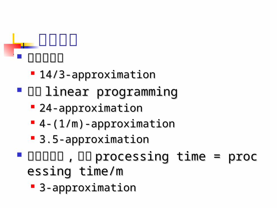
放寬限制 改成可搶先改成可搶先

14/3-approximation14/3-approximation 改成改成 linear programminglinear programming

24-approximation24-approximation 4-(1/m)-approximation4-(1/m)-approximation 3.5-approximation3.5-approximation

改成可搶先改成可搶先 ,, 並且並且 processing time = procprocessing time = processing time/messing time/m 3-approximation3-approximation

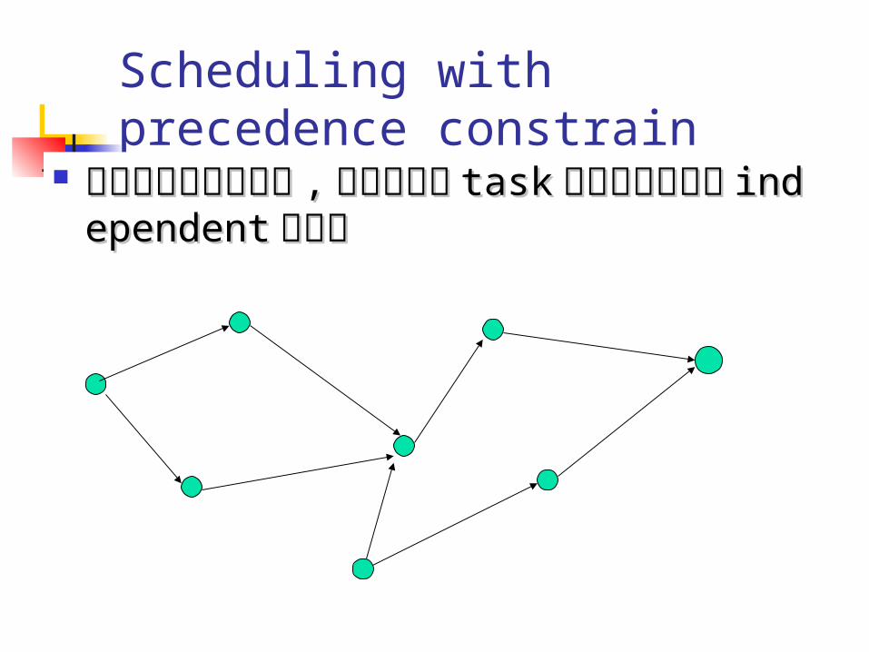
Scheduling with precedence constrain

問題和之前的差不多問題和之前的差不多 ,, 只不過各個只不過各個 tasktask 之之間已經不再是間已經不再是 independentindependent 的關係的關係

困難度 Single machineSingle machine 的狀況的狀況

Without release dates Without release dates NP-hard NP-hard 2-approximation2-approximation

With release datesWith release dates 2.718-approximation2.718-approximation

m-Machinem-Machine 的狀況的狀況 Without release dates & precedence constraWithout release dates & precedence constra

in in NP-hard NP-hard Without weights and precedence graph is uWithout weights and precedence graph is u

nion of chain nion of chain NP-hard NP-hard

On machine scheduling

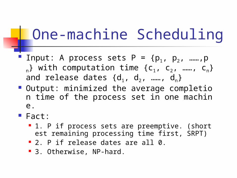
One-machine Scheduling Input: A process sets P = {p1, p2, ……,pn} wit

h computation time {c1, c2, ……, cn} and release dates {d1, d2, ……, dn}

Output: minimized the average completion time of the process set in one machine.

Fact: 1. P if process sets are preemptive. (shortest re

maining processing time first, SRPT) 2. P if release dates are all 0. 3. Otherwise, NP-hard.

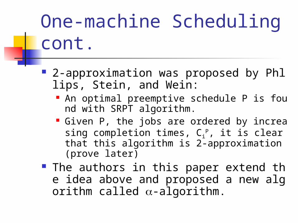
One-machine Scheduling cont. 2-approximation was proposed by Phllips,

Stein, and Wein: An optimal preemptive schedule P is found with

SRPT algorithm. Given P, the jobs are ordered by increasing com

pletion times, CiP, it is clear that this algorithm is

2-approximation (prove later) The authors in this paper extend the idea a

bove and proposed a new algorithm called -algorithm.

Algorithm Algorithm:

Given a preemptive schedule P and (0, 1], define Cj

P() to be the time at which pj, an fraction of Jj, is completed.

Execute the process according to the sorted CjP()

Clearly, an algorithm is either on-line or off-line. Observation:

1. The algorithm is either on-line or off-line 2.if = 1, this algorithm is the same as previous al

gorithm.

Algorithm cont. Approximation analysis:

1. Is it P? 2. Is it feasible? 3. It’s approximation ration? 1+1/, will prove l

ater. 4. Tight? Yes

The weighted version doesn’t improved. Fact:4/3 approximation with preemptive algo. Fact:2.12 for non-preemptive algo.

One-machine scheduling with release dates

Let P be a preemptive schedule, and denote the completion time of Ji in P and in the nonpreemptive -schedule derived from P, respectively

Theorem 2.1: Given an instance of one-machine scheduling with release dates, for any (0,1], an -schedule has

further, there are instances where the inequality is asymptotically tight.

CP

i C i

j

p

jj

j CC )1

1(

Proof of Theorem 2.1(1/2) index the jobs by the order of their

-points in the preemptive schedule P.

let be the latest release date among jobs with points no greater than j’s

By time , jobs 1 through j have all been released, hence

………………(2.1)

rr kjkj 1

maxmax

r jmax

j

kkjj prC

1

max

Proof of Theorem 2.1(2/2) ,since only an fraction j ha

s finished by , since fractions of job

1,..,j must run before time

(2.1)

j

k k

P

j pC 1

rC j

P

j

max

r jmax

CP

j

j

kk

P

j

j

kk

P

j pCpC11

1

j

kkjj prC

1

max

CCP

j

P

j 1

CP

j)

11(

j

P

jj j CC )1

1(

Tightness of theorem 2.1

P0=1

0 - +

P1= P2=...=Px+1 = 0

x jobs

P0 P0

1

P2...Px+1

P0

1+

)1(0

CP C

P

1 CCP

x

P

12... points:

P1

1+

P1

P2...Px+1+x(+)+(1+)

+(1+)+x(1+ )

Optimal:

schedule: as x>>1, ->0, ratio -> 1

1

P0

more about theorem 2.1

since (0,1], this theorem yields approximation bounds that are worse than 2.

However, we will introduce a new fact that ultimately yield better algorithms that makespan of an -schedule is within a (1+ )-factor of the makespane of the corresponding preemptive schedule.

j

P

jj j CC )1

1(

more about theorem 2.1 The idle time introduced in the nonpr

eemptive schedules decrease as is reduced from 1 to 0.

The (worst-case) bound on the completion time of any specific job increase as goest from 1 to 0.

It is the balancing of these two effects that leads to better approximations.

refinement of theorem 2.1 Let denote the set of jobs which complet

e exactly fraction of their processing time before in the schedule P, P is a preemptive schedule. (Ji is included in ).

we also overload to denote the sum of processing times of all jobs in the set

Let Ti be the total idle time in P before Ji completes.

SP

i

CP

i

1SP

i

SP

i

SP

i

refinement of theorem 2.1

Preemptive completion time of Ji can be written as the sum of the idle time and fractional processing times of jobs that ran before .

lemma2.2We next upper bound the completion time

of a job Ji in the -schedule. lemma 2.3

10 SC

P

ii

P

iT

CP

i

SSCP

i

P

iiiT )1(

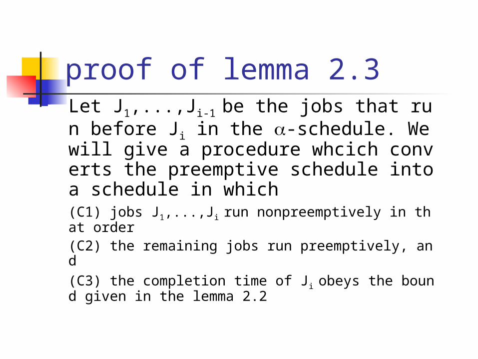
proof of lemma 2.3 Let J1,...,Ji-1 be the jobs that run before

Ji in the -schedule. We will give a procedure whcich converts the preemptive schedule into a schedule in which(C1) jobs J1,...,Ji run nonpreemptively in that order(C2) the remaining jobs run preemptively, and(C3) the completion time of Ji obeys the bound given in the lemma 2.2

proof of lemma 2.3

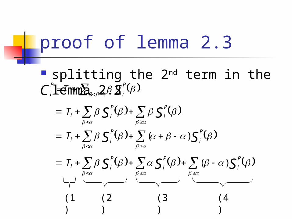
splitting the 2nd term in the lemma 2.2

10 SCP

ii

P

iT

SSP

i

P

iiT

SSP

i

P

iiT )(

SSSP

i

P

i

P

iiT )(

(1) (2) (3) (4)

proof of lemma 2.3 Let JB = and JA = J – JB

(1) the idle time in the preemptive schedule before

(2) the pieces of jobs in JA hat ran before(3) for each job Jj JB, the pieces of Jj t

hat ran before (4) for each job Jj JB, the pieces of Jj t

hat ran between and

S

P

i

CP

i

CP

i

CP

j

CP

j CP

i

proof of lemma 2.3

Let xj be the for which Jj ,that is, the fraction of Jj that was completed before

(xj - )pj is the fraction of job Jj that ran between and

SP

i

CP

i

jJJ j

P

ipxB

jS )()(

CP

j CP

i

proof of lemma 2.3

Let JC = {J1,...,Ji}, the jobs that run no later than Ji in -schedule.

Thus, JC JB

Now, think of schedule P as an ordered list of pieces of jobs (with size).

ikCCP

i

P

k,...,1

SP

i

BJnote :

proof of lemma 2.3

for each Jj JC modify the list by 1. removing all pieces of jobs that run between

and 2.inserting a piece of size (xj - )pj at point corre

sponding to now, we have pieces of size (xj - )pj of jobs j1,...ji

in the correct order (plus other pieces of jobs) convert this ordered list back into a schedul

e by scheduling the pieces in the order of the list, respecting release dates.

claim that ji still completes at time

CP

j

CP

i

CP

j

CP

i

0 time

Job1

Job2

Job3

Job4

schedule by release dates

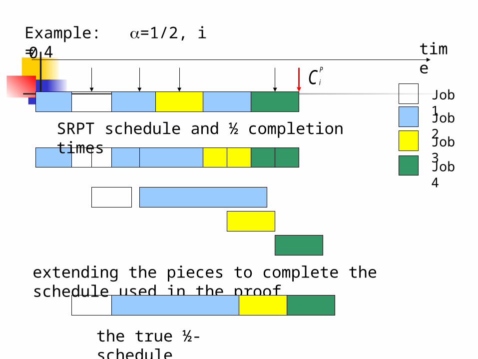
Example: =1/2, i = 4

SRPT schedule and ½ completion times

after 1. 2.

CP

i

proof of lemma 2.3 the total processing time before rem

ains unchanged and that other than the pieces of size (xj - )pj , we moved pieces only later in time, so no additional idle time need be introduced.

for each job Jj JC, extend the piece of size (xj - )pj to one of size pj by adding pj - (xj-)pj units of processing and replace the pieces of Jj that occur earlier, of total size pj, by idle time.

CP

i

0 time

Job1

Job2

Job3

Job4

Example: =1/2, i = 4

SRPT schedule and ½ completion times

CP

i

extending the pieces to complete the schedule used in the proof

the true ½-schedule

proof of lemma 2.3

the completion time of Ji is

B

jC

j JJjjj

P

iJJ

jjj

P

ipxppxp CC

SCP

i

P

i

1

SSP

i

P

iiT 1 ..........lemma 2.2

...........reindexing j by

proof of lemma 2.3

To complete the proof, observe that the remaining pieces in the schedule are all from jobs in J- JC, and we have thus met the conditions (C1),(C2),(C3) above.

applying lemma 2.3 to the last job to complete in the -schedule yields the corollary 2.4

corollary 2.4

The makespan of the -schedule is at most (1+ ) times the makespan of the corresponding preemptive schedule, and there are instances for which this bound is tight.

Random- Algorithm Observation: a key observation is that a

worse-case instance that induces a performance ration 1+1/ is not a worse-case instance for many other values of .

The previous observation suggests the authors to develop a randomized algorithm to pick randomly.

The authors propose on-line algorithm with expected 1/(e-1) approximation and off-line algorithm with 1/(e-1) approximation.

Random- Algorithm cont. According to previous lemma, the approximation r

atio is going to depend on the distribution of the different sets Si

P(). To avoid the worse case , we choose randomly

according to some probability distribution. Lemma 2.5: suppose is chosen from a probability

distribution over (0, 1] with a density function f. Then for each job Ji, E[Ci

] (1+) CiP. It follows that E

[iCi] i(1+) Ci

P.

df

010)(

1max

Random- Algorithm cont.

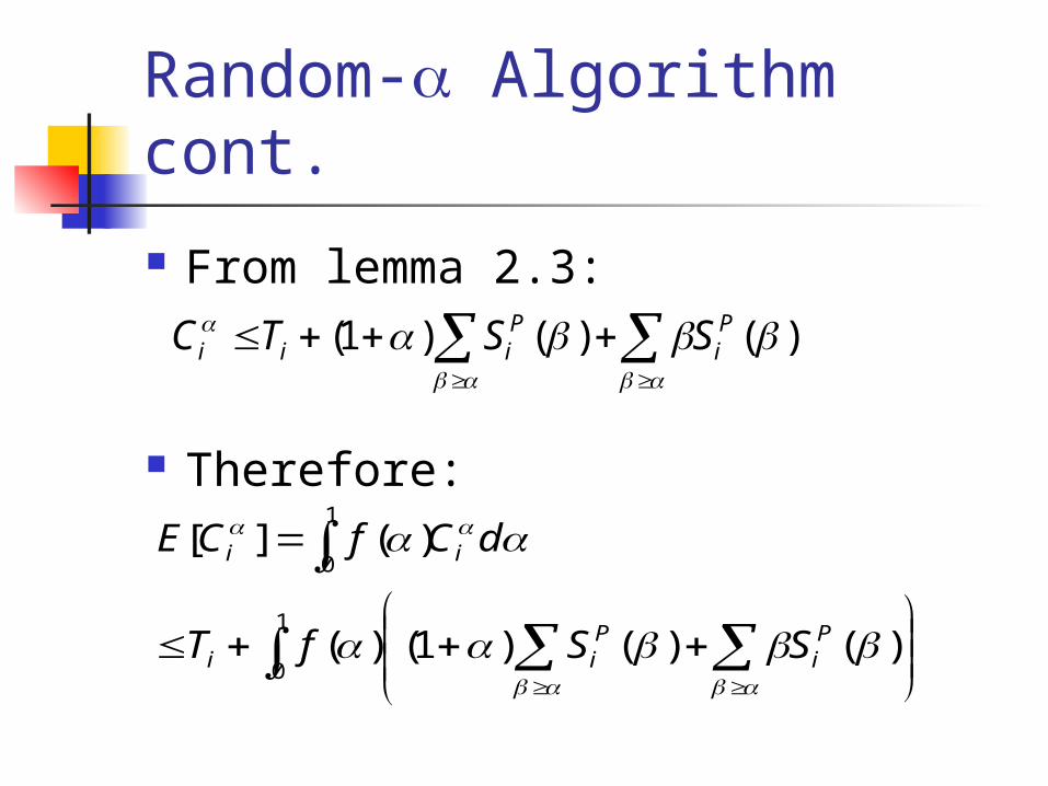
From lemma 2.3:

Therefore:

)()()1( Pi

Piii SSTC

)()()1()(

)(][

1

0

1

0

Pi

Pii

ii

SSfT

dCfCE

11

11010

100

1000

10

1

0

1

0

)()1(

)()(1

max1

)(1

1)(

))(1()()1()(

)()()1()(

)()(1)(

Pi

Pi

Pi

Pi

Pi

Pi

Pi

S

Sdf

dfS

dfdfS

dfdfS

dSSf

Random- Algorithm cont. According to lemma 2.2 and lemma 2.5,

it follows that

Using linearity of expectations, the expected total completion time of schedule is within (1+) of the preemptive schedule’s total completion time.

Pi

Piii CSTCE )1()()1(][

10

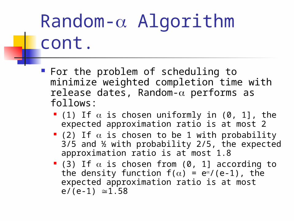
Random- Algorithm cont. For the problem of scheduling to minimize

weighted completion time with release dates, Random- performs as follows: (1) If is chosen uniformly in (0, 1], the

expected approximation ratio is at most 2 (2) If is chosen to be 1 with probability 3/5

and ½ with probability 2/5, the expected approximation ratio is at most 1.8

(3) If is chosen from (0, 1] according to the density function f() = e/(e-1), the expected approximation ratio is at most e/(e-1) 1.58

Random- Algorithm cont. Proof of (1): choosing uniformly corresponds

to the f() = 1, according to lemma 2.5, the we get an approximation ratio of 2.

22

11(max1

2

1)

1(max1

1max1

1max1

10

10

0010

010

dd

d

Random- Algorithm cont.

Proof of (3)

1

1)(

)1(

1

)11()1(

1

)1()1(

1)

1

1(

1

))(()1(

1)

1(

1

)1

(1

)1

(1

)1

(1

00

00

0

ee

eeeee

eeee

e

eeee

e

de

ed

e

e

de

e

Random- Algorithm cont.

=1/e-1 1+1/(e-1) e/(e-1) Proof of (2): omitted The density function e/(e-1) minimize

over all choices of f().

Best- Algorithm In the off-line setting, rather than choosing

randomly, we can try different values of and choose the one that yields the best schedule. This is called Best- scheduling.

Corollary: Algorithm Best- is an e/(e-1)-approximation algorithm for non-preemptive scheduling to minimize average completion time on one machine with release dates. It runs O(n2) time.

Best- Algorithm cont. Approximation ratio follows from previous theore

m. The SRPT schedule preempts only at release dates

so that it has at most n-1 preemptions and there are at most n combinatorially distinct value of for a given preemptive schedule.

The SRPT schedule can be computed in O(nlogn) time using a simple priority queue and given the schedule and an . The corresponding -schedule can be computed in linear time by a simple scan.

On-line Random- Scheduling Theorem: There is a polynomial-time randomized

on-line algorithm with an expected competitive ratio e/(e-1) for the problem of minimizing total completion time in the presence of release dates.

The algorithm picks an (0,1] according to the density function f(x) = ex/(e-1) before receiving any input.

The algorithm simulates the on-line preemptive SRPT schedule. At the exact time when a job finishes a fraction of its processing time in the simulated SRPT schedule, it is added to the queue of jobs to be executed non-preemptively.

On-line Random- Scheduling cont.

The non-preemptive schedule is obtained by executing jobs in the strict order in the queue.

This is a valid on-line scheduling. The bound on the expected competitive ratio

is the same as theorem 2.6. Since lemma 2.3 does not apply the true schedule, but a weaker one in which for every job Ji the first fraction of its processing time in the SRPT schedule is left as idle time.

Negative Results

There are negative results for the various algorithm 1. If is chosen uniformly, the

expected approximation ratio is at least 2

2. For the Best- algorithm, the approximation ratio is at least 4/3

Negative Result cont. Proof of (1):

I(, n): (t(0), p(1)), n jobs (t(), p(0)) Optimal preemptive schedule: 1+n. Optimal non-preemptive schedule:n+1+ There are only two combinatorially distinct schedules cor

responding to the values of , > Let S1 and S2 be the two schedules and C1 and C2 be their t

otal completion times, C1 = 1+n, C2 = n+1+ If is chosen uniformly at random, S1 is chosen with pro

bability and S2 with the probability (1- ), (1+n) + (n+1+) (1- ) = 1+ +2n- 2- n2

Choose n>>1 and <<1 the expected ratio is approach 2

Negative Result cont. Proof of (2):

Add n jobs (t(1), p(0)) to the previous I(1/2, n). Optimal preemptive schedule: 1+3/2n Optimal non-preemptive schedule 2+3n/2 There are only two combinatorially distinct schedule

s corresponding to the values of 1/2, > 1/2 Let S1 and S2 be the two schedules and C1 and C2 be t

heir total completion times, C1 = 1+2n, C2 = 3/2+2n. The approximation ratio is at least 4/3

Improvement

Stougie and Vestjens improved the lower bound for randomized on-line algorithm to e/(e-1)

The tight instance of Best- algorithm was proposed by Torng and Uthaisombut..

Parallel machine scheduling with release dates

TaskTask 的的 propertyproperty Release timeRelease time Processing timeProcessing time weightweight

執行環境執行環境 mm 個個 machinemachine

目標目標 讓讓 average weighted completion timeaverage weighted completion time 最小最小化化

m-Machine Scheduling

將問題轉換到 single-machine 假設假設 MultiMulti 為原問題為原問題 ,Single,Single 為轉換到為轉換到 singlsingl

e-machinee-machine 上的問題上的問題 ,, 那麼…那麼… SingleSingle 中的中的 tasktask 數目和數目和 MultiMulti 一模一樣一模一樣 SingleSingle 中所有中所有 tasktask 的執行時間為原先的的執行時間為原先的 1/m1/m

ppjj’ = p’ = pjj/m/m SingleSingle 中所有中所有 tasktask 的準備好時間的準備好時間 (ready time)(ready time)跟原本一樣跟原本一樣

rrjj’= r’= rjj

Lemma 3.1 The value of an optimal solution to “SinThe value of an optimal solution to “Sin

gle” is a lower bound on the value of an gle” is a lower bound on the value of an optimal solution to “Multi”optimal solution to “Multi”

證明：使用證明：使用 time sharingtime sharing 的方法證明即可的方法證明即可

Completion time 的觀察

max1

1

1 1

1

1

'max

'

''

jkjkpj

j

k

j

k

kk

pj

jjPj

rrC

m

ppC

prC

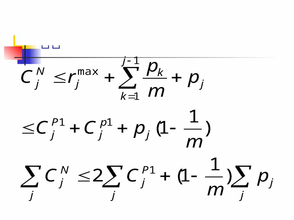
證明

jj

j

Pj

j

Nj

jpj

Pj

j

kj

kj

Nj

pm

CC

mpCC

pm

prC

)1

1(2

)1

1(

1

11

1

1

max

證明 By lemma 3.1By lemma 3.1 我們可以得到二個式子我們可以得到二個式子

因此就可以得到我們想要的結果因此就可以得到我們想要的結果 (3-1/m)-a(3-1/m)-approximationpproximation

jjj

j jj

Pj

Cp

CC

*

*1

Scheduling algorithms with precedence constrain

Agenda

DELAY LIST Algorithm Definition Some Lemma. Theorem

One-machine relaxation Generic m-machine schedule

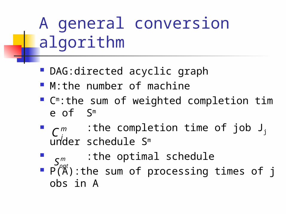
A general conversion algorithm

DAG:directed acyclic graph M:the number of machine Cm:the sum of weighted completion time of S

m

:the completion time of job Jj under schedule Sm

:the optimal schedule P(A):the sum of processing times of jobs in A

mjC

moptS

Definition

For any vertex J,recursively define the quantity κj as follows. For a vertex j with no predecessors κj = pj + rj. Otherwise define κj = pj + max{max i<j κj , rj}. Any path Pij form i to j where p(Pij)= κj is referred to as a critical path to J.

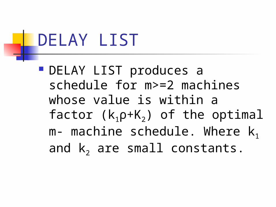
DELAY LIST

DELAY LIST produces a schedule for m>=2 machines whose value is within a factor (k1ρ+K2) of the optimal m- machine schedule. Where k1 and k2 are small constants.

DELAY LIST(cont.) The one-machine schedule taken as a

list (jobs in order of their completion times in the schedule) provides some priority information on which jobs to schedule earlier.

When trying to convert the one-machine schedule into an m-machine one, precedence constraints prevent complete parallelization.

DELAY LIST(cont.) If all pi are identical (say 1), we can afford to

use naive list scheduling. if not all pi ’s are the same, a job could keep a

machine busy, delaying more profitable jobs that become available soon. At the same time, we cannot afford to keep machines idle.

schedule a job out-of-order only if there has been enough idle time already to justify scheduling it.

A job is ready if it has been released and all its predecessors are done.

Definition 4.2.

The time at which job Ji is ready in a schedule S is denoted by qS

i and the time at which it starts is denoted by sS

i .

Charge Schema

1. There is an idle machine M and the first job Jj on the list is ready at time t—schedule Jj on M and charge all uncharged idle time in the interval (qm

j , smj )to Jj .

2. There is an idle machine and the first job Jj in the list is not ready at t, but there is another ready job on the list—focusing on the job Jk which is the first in the list among the ready jobs, schedule it if there is at least βpk uncharged idle time among all machines and charge βpk idle time to Jk.

3. There is no idle time or the above two cases do not apply—do not schedule any job; merely increment t.

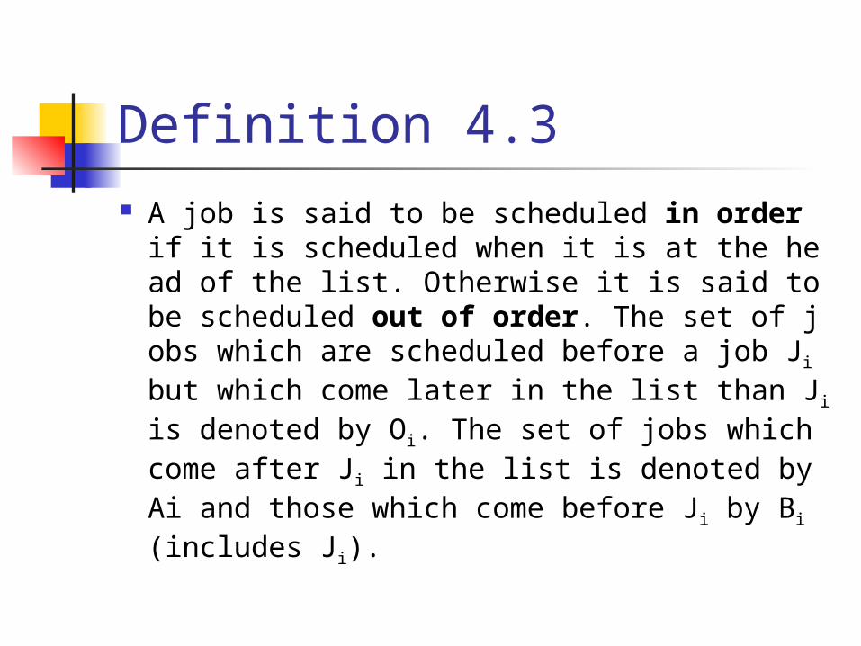
Definition 4.3 A job is said to be scheduled in order if it is

scheduled when it is at the head of the list. Otherwise it is said to be scheduled out of order. The set of jobs which are scheduled before a job Ji but which come later in the list than Ji is denoted by Oi. The set of jobs which come after Ji in the list is denoted by Ai and those which come before Ji by Bi (includes Ji).

Definition 4.4

For each job Ji , define a path P i = Jj1, Jj2, . . . , Jjl , with Jjl =Ji with respect to the schedule Sm as follows. The job Jjk is the predecessor of Jjk+1 with the largest completion time (in Sm) among all the predecessors of Jjk

+1 such that Cmjk ≥ rjk+1; ties are broken arbitrarily. Jj1 i

s the job where this process terminates when there are no predecessors which satisfy the above condition. The jobs in Pi’ define a disjoint set of time intervals (0, rj1 ], (sm

j1, Cmj1 ], . . . , (sm

jl, Cmjl ] in the schedule. Le

t κi’ denote the sum of the lengths of the intervals.

Fact

Fact 4.5. κi’ ≤ κi

Fact 4.6. The idle time charged to each job Ji is less than or equal to βpi

Lemma 4.7 A crucial feature of the algorithm is that wh

en it schedules jobs, it considers only the first job in the list that is ready, even if there is enough idle time for other ready jobs that are later in the list.

For every job Ji , there is no uncharged idle time in the time interval (qm

i , smi ), and furth

ermore all the idle time is charged only to jobs in Bi.

Lemma 4.8

For every job Ji , the total idle time charged to jobs in Ai , in the interval (0, sm

i

), is bounded by m(κi’ - pi). It follows that p(Oi) ≤ m(κi’ - pi)/β ≤ m(κi - pi)/β.

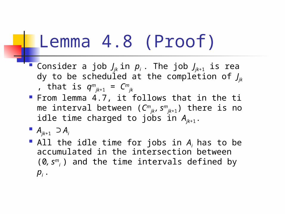
Lemma 4.8 (Proof) Consider a job Jjk in pi . The job Jjk+1 is ready to b

e scheduled at the completion of Jjk , that is qmjk

+1 = Cmjk

From lemma 4.7, it follows that in the time interval between (Cm

jk , smjk+1) there is no idle time ch

arged to jobs in Ajk+1. Ajk+1 ⊃ Ai All the idle time for jobs in Ai has to be accumul

ated in the intersection between (0, smi ) and th

e time intervals defined by pi .

Lemma 4.8 (Proof)

bounded by m(κi’ - pi). total processing time of the jobs in Oi i

s bounded by 1/β times the total idle time that can be charged to jobs in Ai

mOpBpBpKttC iiiimi /))()()(('21

'/)'(/)()1( iiii KpKmBp

i

ii

PKmBP ')

11(/)()1(

Theorem 4.9

Let Sm be the schedule produced by the algorithm Delay List using a list S1. Then for each job Ji , Cm

i ≤ (1+ β)p(Bi)/m + (1 + 1/β)κi’ - pi

/β.

Theorem 4.9(proof)

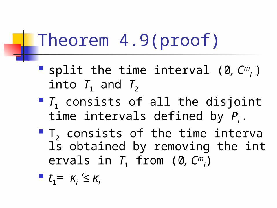
split the time interval (0, Cmi ) into T1 an

d T2 T1 consists of all the disjoint time interv

als defined by Pi . T2 consists of the time intervals obtaine

d by removing the intervals in T1 from (0, Cm

i) t1= κi ‘≤ κi

Theorem 4.9(proof) From Lemma 4.7, in the time intervals

of T2, all the idle time is either charged to jobs in Bi, and the only jobs which run are from Bi∪Oi

From Fact 4.6, the idle time charged to jobs in Bi is bounded by βp(Bi).

t2 is bounded by (βp(Bi) + p(Bi) + p(Oi))/m

One –machine relation The following two lemmas provide lower bo

unds on the optimal m-machine schedule in terms of the optimal one-machine schedule.

This one-machine schedule can be either preemptive or non-preemptive; the bounds hold in either case.

Lemma 4.10. Cmopt ≥ C1

opt / m Lemma 4.11. Cm

opt ≥ ∑iwiκi = C∞opt

Lemma 4.10

Cmopt ≥ C1

opt / m Prof:

If i <j , then Cmi ≤ sm

j ≤ Cmj which implies that the

re will be no precedence violations in S1. Claim for every job Ji , C1

i ≤ mCmi

P : the sum of the processing times of all the jobs which finish before Ji (including Ji) in Sm.

I : the total idle time in the schedule Sm before Cm

i .

Lemma 4.10(proof)

mCmi ≥ P + I

The idle time in the schedule S1 can be charged to idle time in the schedule Sm

P is the sum of all jobs which come before Ji in S1.

C1i ≤ P + I

Lemma 4.11

Cmopt ≥ ∑iwiκi = C∞

opt Prof:

The length of the critical path κi is an obvious lower bound on the completion time Cm

i of job Ji if the number of machines is unbounded,

every job Ji can be scheduled at the earliest time it is available and will finish by κi

Generic m-machine schedule Let Sm be the schedule produced by the alg

orithm Delay List using a one-machine schedule S1 as the list. Then for each job Ji ,

Cmi ≤ (1 + β)C1

i /m + (1 + 1/β)κi Proof:

Form theorem 4.9 :Cmi ≤ (1+ β)p(Bi)/m + (1 + 1/β)κi

’ - pi /β. P(Bi)<=C1

i ; Ki’<=Ki

Theorem 4.13

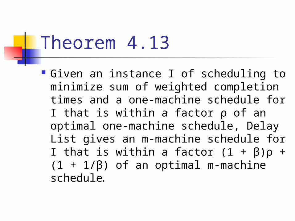
Given an instance I of scheduling to minimize sum of weighted completion times and a one-machine schedule for I that is within a factor ρ of an optimal one-machine schedule, Delay List gives an m-machine schedule for I that is within a factor (1 + β)ρ + (1 + 1/β) of an optimal m-machine schedule.

Theorem 4.13(proof)

i

i

ii

i

mii

m Km

CWCWC

1

111

iii

iii KWCW

m 1

11 1

OPTOPTm C

m

CC

11 1

mOPTC

1

11

i OPTii CCWC 111

Conclusions 論文中於論文中於 conclusionconclusion 這一個小節中談論到這一個小節中談論到最新的研究成果最新的研究成果 ,, 包括這個問題是否有包括這個問題是否有 PTAPTASS 的方法…的方法…

將問題參數化將問題參數化 由於原問題在不同的參數下會有不一樣的結果由於原問題在不同的參數下會有不一樣的結果 ,,因此只要在憑藉著優異的數學技巧因此只要在憑藉著優異的數學技巧 ,, 就可以得就可以得到一個更好的演算法到一個更好的演算法

Optimal solutionOptimal solution 的定義的定義 這篇論文常常把可搶先的這篇論文常常把可搶先的 solutionsolution 定義為定義為 OPT,OPT,雖然實際上不是如此雖然實際上不是如此 ,, 但是為了證明也只好如但是為了證明也只好如此此