cash holdings: evidence from firm-level big data …cash holdings: evidence from firm-level big data...
TRANSCRIPT
〈内閣府経済社会総合研究所『経済分析』第 200 号 2019 年〉
135
Cash Holdings: Evidence from Firm-Level Big Data in Japan*
By Kaoru HOSONO, Daisuke MIYAKAWA and Miho TAKIZAWA**
Abstruct
To investigate the status of Japanese firms’ cash holdings, first, we document how the dis-tribution of firms’ cash holding has been evolving over the last two decades. Our descriptive analyses using Japanese firm-level “big data” accounting for at most 400 thousand firms over the period of 1994-2016 suggest that Japanese firms on average have increased its size-adjusted cash holding since the late 2000s. This trend has been accompanied by increasing dispersion of the size-adjusted cash holding among firms. Second, we document how firms have increased their cash holdings. The results of our panel estimation show that the sensitivity of the change in cash holdings with respect to the change in cash inflow becomes substantially larger since the late 2000s. Such a sensitivity is also found to be larger for firms holding small-er account receivables and/or inventory as well as for firms with smaller number of customer or transacting with customer showing worse creditworthiness. These results suggest firms’ het-erogeneous motivations to hold cash, i.e., firms’ recent tendency to hold larger cash is found for the firms facing better business conditions and keeping better financial position (i.e., smaller demand for working capital), but driven also by precautionary saving motive.
JEL classification: E22, G31, G32 Keywords: Cash Holdings, Cash Inflow, Precautionary Motive
* Hosono: Faculty of Economics, Gakushuin University, kaoru.hosono(at)gakushuin.ac.jp; Miyakawa (corre-sponding author): Hitotsubashi University Business School, dmiyakawa(at)hub.hit-u.ac.jp; Takizawa: Faculty of Economics, Gakushuin University, miho.takizawa(at)gakushuin.ac.jp. This research was conducted as a part of the Economic and Social Research Institute (ESRI) research project (Revitalizing the economy: Structural challenges faced by firms and households). We would like to thank Wako Watanabe, Tatsuo Senga, Johannes Wieland, Takashi Unayama, Arito Ono, Nobuo Kagomiya, Etsuro Shioji, and the participants of a seminar at ESRI for their helpful suggestions. Miyakawa gratefully acknowledges financial supports from the Grant-in-Aid for Scientific Research No. 16K03736 and 17H02526 from the grant-in-aid from Zengin Foundation for Studies on Economics and Finance as well as the generous data provision by Tokyo Shoko Research (TSR), Ltd. through the collaborative research works between Hitotsubashi University and TSR. **細野 薫:学習院大学経済学部経済学科教授 kaoru.hosono(at)gakushuin.ac.jp、宮川 大介(責任著者):
一橋大学大学院経営管理研究科准教授 dmiyakawa(at)hub.hit-u.ac.jp、滝澤 美帆:学習院大学経済学部経
済学科教授 miho.takizawa(at)gakushuin.ac.jp.
論 文
『経済分析』第 200号
134
図表 A-4 被取得事業セグメントと主要既存事業セグメントの買収後利益率
- 134 - - 135 -

『経済分析』第 200 号
136
日本企業の現金保有行動 : 大規模企業レベルパネルデータを用いた実証分析
滝澤 美帆・細野 薫・宮川 大介
<要旨>
本稿では、日本企業の現金保有行動について、1994 年から 2016 年の期間に亘る最大 40
万社からなる企業レベルの大規模パネルデータを用いて実証的に検討した。得られた結果
は、以下の通りである。第一に、日本企業の現金保有比率(対総資産及び対売上高)は 2000
年代後半から平均的に上昇しているが、同時にそのばらつきも拡大している。第二に、こ
うした現金保有比率の平均的な上昇に際して、現金保有比率のキャッシュインフローに対
する感応度が上昇している。また、こうした傾向は、運転資金需要が低く企業金融面で有
利なポジションにあると考えられる企業でより顕著である一方、信用力の乏しい少数の販
売先を顧客として抱えている企業においてもまた強く確認される。これらの結果は、近年
における日本企業の現金保有比率の上昇傾向が、良好な企業業績と金融環境を背景として
いる一方、依然として予備的貯蓄動機に基づく現金保有行動も窺えるなど、個々の企業の
異質な動機を反映したものであることを示唆している。
JEL classification: E22, G31, G32
Keywords: 現金保有、キャシュインフロー、予備的貯蓄動機
- 136 -

Cash Holdings: Evidence from Firm-Level Big Data in Japan
137
1.Introduction
Corporate savings have been reported to exhibit an increasing trend in many countries in-cluding the US, Japan, Germany and China. Karabarbounis and Neiman (2012) show that 30 out of the 44 countries with more than 10 years of data exhibited increasing trends in the share of saving in corporate sector. Such an increase in corporate savings is accompanied by an in-crease in corporate holdings of cash. Bates et al. (2009), among others, show that the average cash-to-assets ratio of the US corporations increased by 0.46% per year from 1980 to 2006. Given an increasing trend of corporate savings and cash holdings have significant impacts on the flow of funds, and thereby on corporate investment, tax revenues, and distribution of wealth, understanding what drives such dynamics of corporate savings has been one of the most important issues from the viewpoints of policymakers, practitioners, and academic re-searchers.
Against this background, it has still been an open question both from practical and aca-demic perspectives why firms hold more cash than they used to do. The extant studies have been mainly hypothesizing that firms need to hold liquidity as they are facing financial friction, and attempting to test if this is the case. To proxy for the degree of financial friction, the extant literature has employed, for example, firms’ leverage, cash-flow uncertainty, relationship to their lender banks, and so on. While these mechanism is intuitive, there are several details missed in the extant discussions. Among many, we think it is important to explicitly analyze how firm-to-firm trade and the relationship between firms and their transaction partners matter for cash holding. To illustrate, firms transacting with a larger number of transaction partners are supposed to be less worried about the default or the product disruption of one of those, thus do not necessarily hold large amount of cash. We think it is informative to empirically examine such a relationship between firms’ cash holdings and transaction relationships.
Toward this end, first, we use Japanese firm-level big data accounting for at most 400 thousand firms per a year over twenty three years from 1994 to 2016, and document how the distribution of firms’ cash holding has been evolving over those two decades. Our descriptive analyses suggest that since the late 2000s, firms on average increased its intensity of cash holding represented by the ratio of cash to firm size (e.g., total assets or sales). This trend has been also accompanied by increasing dispersion of cash holding among firms. We report that such a pattern is robust against the employment of various firm size measures (e.g., total assets or sales) and the restriction of our data to balanced panel data. This fact implies while the re-cent trend of higher cash holding is firmly confirmed on average, there is also a substantial degree of firm-level heterogeneity in terms of the level of cash holding and it has been magni-fied recently.
『経済分析』第 200 号
136
日本企業の現金保有行動 : 大規模企業レベルパネルデータを用いた実証分析
滝澤 美帆・細野 薫・宮川 大介
<要旨>
本稿では、日本企業の現金保有行動について、1994 年から 2016 年の期間に亘る最大 40
万社からなる企業レベルの大規模パネルデータを用いて実証的に検討した。得られた結果
は、以下の通りである。第一に、日本企業の現金保有比率(対総資産及び対売上高)は 2000
年代後半から平均的に上昇しているが、同時にそのばらつきも拡大している。第二に、こ
うした現金保有比率の平均的な上昇に際して、現金保有比率のキャッシュインフローに対
する感応度が上昇している。また、こうした傾向は、運転資金需要が低く企業金融面で有
利なポジションにあると考えられる企業でより顕著である一方、信用力の乏しい少数の販
売先を顧客として抱えている企業においてもまた強く確認される。これらの結果は、近年
における日本企業の現金保有比率の上昇傾向が、良好な企業業績と金融環境を背景として
いる一方、依然として予備的貯蓄動機に基づく現金保有行動も窺えるなど、個々の企業の
異質な動機を反映したものであることを示唆している。
JEL classification: E22, G31, G32
Keywords: 現金保有、キャシュインフロー、予備的貯蓄動機
- 136 - - 137 -

『経済分析』第 200 号
138
Given such empirical illustration, second, we document how firms have increased its cash holdings. To illustrate, firms can increase its cash holdings through larger cash inflow as well as better positions in trade finance (e.g., smaller size of shorter duration for account receiva-bles), selling tangibles, borrowing more, etc. The results of our panel estimation, which takes into account the comprehensive list of those possible channels leading to the changes in cash holdings, show that, the sensitivity of the change in cash holdings with respect to the change in cash inflow becomes substantially larger since the late 2000s. Such a stronger positive correla-tion between the change in cash holdings and cash inflow is confirmed with controlling for other potential sources leading to the change in cash holdings. Such a tendency that better per-formed firms are more likely to accumulate cash, which results in wider dispersion of cash holding among firms becomes more apparent once we include new entrant firms to our analy-sis. Interestingly, based on the analyses using unbalanced panel data including newly entrant firms and exiting firms, in addition to the abovementioned larger cash inflow, larger long-term borrowing and smaller account receivables also contribute to higher cash holding while the change in tangibles become less important to the change in cash holdings. These findings sug-gest that, on the one hand, firms accumulate their cash by taking advantage of better business and financing conditions when they perform better. On the other hand, when firm perform worse, they conversely show the decline in cash holding. We should note that such polarization of firms in terms of cash holding (i.e., “second moment”) emerged at the same time as the av-erage increasing trend (i.e., “first moment”) in cash holdings.
Given the abovementioned unconditional linkage between cash inflow and cash holdings over the recent periods, we further take into account firm-level heterogeneity in terms of firms’ balance sheet conditions. Somewhat surprisingly, our empirical results suggest that firms holding smaller account receivables and/or inventory (and larger account payables) in fact tend to show higher sensitivity of the change in cash holdings with respect to cash inflow over the recent periods. This result suggests that firms facing smaller demand for working capital are more likely to secure larger amounts of cash. Such a fact is surprising given the extant discus-sion considering financial friction as the determinants of cash holding. Namely, if firms are in a better financial position, i.e., smaller demand for working capital, they are not supposed to se-cure larger cash. The abovementioned results would, however, imply those firms in better fi-nancial position are the ones accumulating more cash. As we discuss later, we may need addi-tional mechanisms such as uncertainty faced by firms to reconcile this puzzling result.
Regarding the positive association between financial friction and cash holding, we also confirm that firms with smaller number of transaction partners or transacting with partners showing worse creditworthiness typically show such a higher sensitivity of the change in cash holdings with respect to cash inflow. On the one hand, firms with relatively high cash inflow,
- 138 -
Cash Holdings: Evidence from Firm-Level Big Data in Japan
139
which are able to hold larger cash, tend to show lower cash holdings when the number of their transaction partners is large enough. On the one hand, even firms with relatively low cash in-flow, which are predicted to hold smaller cash, exhibit higher cash holding when they are transacting with smaller number customers.
These results obtained from the conditional estimates suggest that firms’ recent tendency to hold larger cash is driven by heterogeneous motivations. Firms facing better business condi-tions and better financial positions are more likely to accumulate cash. Nonetheless, firms fac-ing precautionary saving motive have been also accumulating cash. We think it is one contri-bution of the present paper to show that these heterogeneous motivations for firms to hold cash have been working behind the dynamics of firms’ cash holding, which is missed in the extant studies.
The rest of the present paper proceeds as follows. Section 2 briefly reviews the related extant literature. Section 3 explains the data we use for our analysis and show empirical find-ings. Section 4 concludes and discusses the future research issues.
2.Related studies
A number of extant studies have investigated the reasons for the increasing trend of cor-porate savings and cash holdings. While different researches put emphasis on different factors, most of the extant studies have been attributing such an increasing trend in firms’ cash holding at least partly to financial constraints that firms face. As one prominent study, Bates et al. (2009) empirically examine the reasons for the increase in the cash-to-assets ratios of US cor-porations from 1980 to 2006, finding that cash ratios increased because firms’ cash flows be-come riskier, firms held fewer inventories and receivables, and firms became increasingly R&D intensive. Their findings are consistent with the theoretical illustration based on firms’ precautionary motive for cash holdings but not with the agency conflicts between managers and shareholders (see Jensen, 1986, among others). Harford et al. (2014) focus on a specific type of liquidity risk: refinancing risk. Using data from US firms from 1980 to 2008, they find that the maturity of firms’ long-term debt has shortened markedly, which suggests a higher risk of refinancing and explains a large fraction of the increase in cash holdings over time.
The present paper is closely related to the literature on how financial constraints lead to cash holdings. As one prominent study, Almeida et al. (2004), using data from US manufactur-ing firms over the 1971 to 2000 period, find that financially constrained firms have a positive propensity to save cash out of cash flows (cash flow sensitivity of cash), while unconstrained firms do not. Denis and Sibilkov (2009) also examine why cash holdings are more valuable for
『経済分析』第 200 号
138
Given such empirical illustration, second, we document how firms have increased its cash holdings. To illustrate, firms can increase its cash holdings through larger cash inflow as well as better positions in trade finance (e.g., smaller size of shorter duration for account receiva-bles), selling tangibles, borrowing more, etc. The results of our panel estimation, which takes into account the comprehensive list of those possible channels leading to the changes in cash holdings, show that, the sensitivity of the change in cash holdings with respect to the change in cash inflow becomes substantially larger since the late 2000s. Such a stronger positive correla-tion between the change in cash holdings and cash inflow is confirmed with controlling for other potential sources leading to the change in cash holdings. Such a tendency that better per-formed firms are more likely to accumulate cash, which results in wider dispersion of cash holding among firms becomes more apparent once we include new entrant firms to our analy-sis. Interestingly, based on the analyses using unbalanced panel data including newly entrant firms and exiting firms, in addition to the abovementioned larger cash inflow, larger long-term borrowing and smaller account receivables also contribute to higher cash holding while the change in tangibles become less important to the change in cash holdings. These findings sug-gest that, on the one hand, firms accumulate their cash by taking advantage of better business and financing conditions when they perform better. On the other hand, when firm perform worse, they conversely show the decline in cash holding. We should note that such polarization of firms in terms of cash holding (i.e., “second moment”) emerged at the same time as the av-erage increasing trend (i.e., “first moment”) in cash holdings.
Given the abovementioned unconditional linkage between cash inflow and cash holdings over the recent periods, we further take into account firm-level heterogeneity in terms of firms’ balance sheet conditions. Somewhat surprisingly, our empirical results suggest that firms holding smaller account receivables and/or inventory (and larger account payables) in fact tend to show higher sensitivity of the change in cash holdings with respect to cash inflow over the recent periods. This result suggests that firms facing smaller demand for working capital are more likely to secure larger amounts of cash. Such a fact is surprising given the extant discus-sion considering financial friction as the determinants of cash holding. Namely, if firms are in a better financial position, i.e., smaller demand for working capital, they are not supposed to se-cure larger cash. The abovementioned results would, however, imply those firms in better fi-nancial position are the ones accumulating more cash. As we discuss later, we may need addi-tional mechanisms such as uncertainty faced by firms to reconcile this puzzling result.
Regarding the positive association between financial friction and cash holding, we also confirm that firms with smaller number of transaction partners or transacting with partners showing worse creditworthiness typically show such a higher sensitivity of the change in cash holdings with respect to cash inflow. On the one hand, firms with relatively high cash inflow,
- 138 - - 139 -

『経済分析』第 200 号
140
financially constrained firms than for unconstrained firms, and conclude that greater cash holdings are associated with higher levels of investment for financially constrained firms with high hedging needs. Their results suggest that greater cash holdings of constrained firms are a natural (value-increasing) response to costly external financing. One of the biggest challenges these researches face is how to classify firms into financially constrained and unconstrained firms. Almeida et al. (2004), for example, use several financial constraints criteria: the payout ratio (the ratio of dividends and stock repurchases to operating income), the asset size, bond ratings, commercial paper ratings, and the Kaplan-Zingales index (Kaplan and Zingales 1997). Although these measures are fairly plausible, they may still suffer from serious endogeneity and selection problems. For example, among the firms that are classified as a financially con-strained due to the lack of bond ratings, there may be firms that do not need external finance due to the lack of investment opportunities as well as those that are really constrained. The present paper at least party aims at contributing the extant studies focusing on financial con-straint by putting a special emphasis on the friction associated with firm-to-firm transaction relationships.
3.Data and empirical findings
3.1 Data In this section, we will go over the data we use in the present study. All the data are pro-
vided by TSR (Tokyo Shoko Research Ltd.), which is one of the largest credit reporting agencies in Japan, through the joint research agreement between TSR and Hitotsubashi University. TSR is a private company operating in the areas of credit research, publishing, and database distribution. The central product TSR provides is the unsolicited-basis company report accounting for the performance of each targeted firm, which they sell to a variety of clients including banks, secu-rity firms, non-financial enterprises, and governmental organizations.
The main data source for this paper is an annual-frequency panel of Japanese firm data accounting for firms’ financial statement information over 1994 to 2016 fiscal year. As each firm could have different accounting periods, we need to classify those different accounting periods into corresponding fiscal year. In the present paper, we treat the accounting periods ending between June of the year t and the May of the year t+1 as the ones corresponding to the fiscal year t. We exclusively focus on the firms accompanied by the financial statement infor-mation.1 1 Another data file provided by TSR covers much larger number of firms than the one we are using in the present paper. Give such a larger data do not contain comprehensive financial statement information, we decide on using the current sample selection criterion.
- 140 -
Cash Holdings: Evidence from Firm-Level Big Data in Japan
141
In addition to the firm-level characteristics, the dataset also includes linked firm-firm pair-level data accounting for firms’ supply chain network. The data comprise of a pair of firm A and B under a transaction relationship, which are identified as of the end of each accounting period. Each pair is accompanied by an identifier specifying the relationship between those two firms (e.g., firm B is a customer, supplier, or shareholder of firm A). We use the data to identify each firms’ transaction relationships in the later section. 3.2 Evolution of cash holding distribution
As a first step of our analysis, we use the abovementioned TSR data to document how the distribution of firms’ cash holding has been evolving over the last two decades. To measure firms’ cash holdings, we employ the ratio of cash to total asset (cash-to-total asset ratio) and the ratio of cash to sales (cash-to-sales ratio). Given the TSR data is unbalanced panel data, we use the following three data configurations alternatively; all the data provided by TSR, the group of firms staying in the TSR data at least 10 years over the twenty three years from 1994 to 2016, and the group of firms always staying in the data over the same periods (i.e., 15,020 firms).
In order to see the evolution of sample size, Figure 1 shows the number of firms catego-rized in the first category (i.e., all data) as well as the second category (i.e., firms staying in the data at least for 10 years). First, we can see the number of firms in the first category largely increased over the 2000s. This is due to the expansion of TSR data coverage, which had been including a larger number of small and medium enterprises. Second, while we can see the same pattern for the second category, the dynamics of the number of firms is much more stable than the first category especially from the late 2000s. This illustration suggests us the necessity to analyze both the whole unbalanced data and the (largely) balanced data because the empirical results based on the whole unbalanced data are more largely reflecting the characteristics of possibly smaller entrants and exit firms possibly worse in terms of their quality. Given this discussion, we compare the empirical results obtained from the three datasets and how each result is robust against the choice of dataset.
The two panels in Figure 2 correspond to the violin plot of the cash-to-total asset ratio (Panel (a)) and the cash-to-sales ratio (Panel (b)) for the all sample firms in each year over five year intervals.
『経済分析』第 200 号
140
financially constrained firms than for unconstrained firms, and conclude that greater cash holdings are associated with higher levels of investment for financially constrained firms with high hedging needs. Their results suggest that greater cash holdings of constrained firms are a natural (value-increasing) response to costly external financing. One of the biggest challenges these researches face is how to classify firms into financially constrained and unconstrained firms. Almeida et al. (2004), for example, use several financial constraints criteria: the payout ratio (the ratio of dividends and stock repurchases to operating income), the asset size, bond ratings, commercial paper ratings, and the Kaplan-Zingales index (Kaplan and Zingales 1997). Although these measures are fairly plausible, they may still suffer from serious endogeneity and selection problems. For example, among the firms that are classified as a financially con-strained due to the lack of bond ratings, there may be firms that do not need external finance due to the lack of investment opportunities as well as those that are really constrained. The present paper at least party aims at contributing the extant studies focusing on financial con-straint by putting a special emphasis on the friction associated with firm-to-firm transaction relationships.
3.Data and empirical findings
3.1 Data In this section, we will go over the data we use in the present study. All the data are pro-
vided by TSR (Tokyo Shoko Research Ltd.), which is one of the largest credit reporting agencies in Japan, through the joint research agreement between TSR and Hitotsubashi University. TSR is a private company operating in the areas of credit research, publishing, and database distribution. The central product TSR provides is the unsolicited-basis company report accounting for the performance of each targeted firm, which they sell to a variety of clients including banks, secu-rity firms, non-financial enterprises, and governmental organizations.
The main data source for this paper is an annual-frequency panel of Japanese firm data accounting for firms’ financial statement information over 1994 to 2016 fiscal year. As each firm could have different accounting periods, we need to classify those different accounting periods into corresponding fiscal year. In the present paper, we treat the accounting periods ending between June of the year t and the May of the year t+1 as the ones corresponding to the fiscal year t. We exclusively focus on the firms accompanied by the financial statement infor-mation.1 1 Another data file provided by TSR covers much larger number of firms than the one we are using in the present paper. Give such a larger data do not contain comprehensive financial statement information, we decide on using the current sample selection criterion.
- 140 - - 141 -

『経済分析』第 200 号
142
Figure 1 Evolution of firm numbers
Note: The x and circle account for the numbers of firms in each category and in each year. For the latter category,
we identify the firms showing up at least 10 times in our annual-frequency data and count how many of those firms are recorded in each year.
Figure 2 Distribution of cash holdings
Panel (a) Panel (b)
Note: The left and right panels depict the violin plots for firms’ cash-to-asset ratio and cash-to-sales ratio, respec-
tively. The plots are made for each year over the five-year intervals.
We can immediately notice that the median level of cash holdings denoted by the white circle in the plots increased over the years regardless of the measures for the cash holdings. Also, the dispersion of the cash holdings become larger over the years.
Given these two features we can observe in Figure 2 could be potentially driven by the inclusion of entrant firms to TSR data, we repeat the same illustration for the more balanced panel data. The upper panels (i.e., (a) and (b)) in Figure 3 use the data of the firms staying in the data at least 10 years while the lower panels (i.e., (c) and (d)) in Figure 3 use the complete-ly balanced samples.
- 142 -

Cash Holdings: Evidence from Firm-Level Big Data in Japan
143
Figure 3 Distribution of cash holdings
Panel (a) Panel (b)
Panel (c) Panel (d)
Note: The two panels in upper and lower row depict the violin plots for firms’ cash-to-asset ratio (left panel) and
cash-to-sales ratio (right panel), respectively. The plots are made for each year over the five-year intervals.
The evolution of the distribution of cash holdings becomes less apparent in the four pan-els in Figure 3 than that in Figure 2. Nonetheless, we can still largely confirm, first, that the median level of the cash holdings represented by the white circle increased since the late 2000s. This is consistent with the increasing trend in firms’ cash holding widely reported in the extant literature. As the second feature, we can also see that the distribution becomes wider. These descriptive analyses suggest that since the late 2000s, firms on average increased its intensity of cash holding represented by the ratio of cash to firm size while such a trend has been also accompanied by increasing dispersion of cash holding among firms. Regardless of whether we use different firm size measures or how we restrict our data to survived firms, we can confirm the same pattern.
To see the evolution of firms’ cash holding more explicitly, we also run the following firm-level panel estimation as in the form of the equation (1), which has cash-to-total asset ra-
『経済分析』第 200 号
142
Figure 1 Evolution of firm numbers
Note: The x and circle account for the numbers of firms in each category and in each year. For the latter category,
we identify the firms showing up at least 10 times in our annual-frequency data and count how many of those firms are recorded in each year.
Figure 2 Distribution of cash holdings
Panel (a) Panel (b)
Note: The left and right panels depict the violin plots for firms’ cash-to-asset ratio and cash-to-sales ratio, respec-
tively. The plots are made for each year over the five-year intervals.
We can immediately notice that the median level of cash holdings denoted by the white circle in the plots increased over the years regardless of the measures for the cash holdings. Also, the dispersion of the cash holdings become larger over the years.
Given these two features we can observe in Figure 2 could be potentially driven by the inclusion of entrant firms to TSR data, we repeat the same illustration for the more balanced panel data. The upper panels (i.e., (a) and (b)) in Figure 3 use the data of the firms staying in the data at least 10 years while the lower panels (i.e., (c) and (d)) in Figure 3 use the complete-ly balanced samples.
- 142 - - 143 -
『経済分析』第 200 号
144
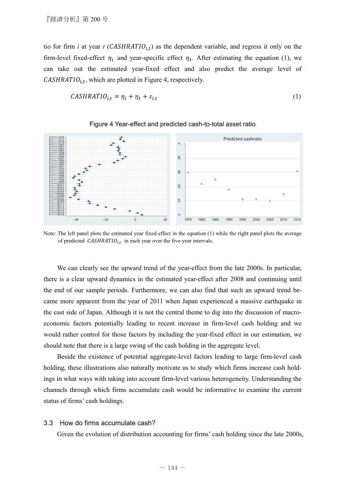
tio for firm i at year t ( ) as the dependent variable, and regress it only on the
firm-level fixed-effect and year-specific effect . After estimating the equation (1), we can take out the estimated year-fixed effect and also predict the average level of
, which are plotted in Figure 4, respectively.
(1)
Figure 4 Year-effect and predicted cash-to-total asset ratio
Note: The left panel plots the estimated year fixed-effect in the equation (1) while the right panel plots the average
of predicted in each year over the five-year intervals.
We can clearly see the upward trend of the year-effect from the late 2000s. In particular, there is a clear upward dynamics in the estimated year-effect after 2008 and continuing until the end of our sample periods. Furthermore, we can also find that such an upward trend be-came more apparent from the year of 2011 when Japan experienced a massive earthquake in the east side of Japan. Although it is not the central theme to dig into the discussion of macro-economic factors potentially leading to recent increase in firm-level cash holding and we would rather control for those factors by including the year-fixed effect in our estimation, we should note that there is a large swing of the cash holding in the aggregate level.
Beside the existence of potential aggregate-level factors leading to large firm-level cash holding, these illustrations also naturally motivate us to study which firms increase cash hold-ings in what ways with taking into account firm-level various heterogeneity. Understanding the channels through which firms accumulate cash would be informative to examine the current status of firms’ cash holdings.
3.3 How do firms accumulate cash?
Given the evolution of distribution accounting for firms’ cash holding since the late 2000s,
- 144 -

Cash Holdings: Evidence from Firm-Level Big Data in Japan
145
we examine how the pattern of accumulating cash changed over time. To illustrate, firms can accumulate cash through various channels ranging from larger cash inflow, shortening the du-ration for account receivables, selling tangibles, borrowing more, and so on. To see the associ-ation between the change in cash-to-total asset ratio and those potential sources for changing the cash holding, we run the following firm-level panel estimation in the form of the equation (2).
������������� � �������������� � ∑ ������������ � �� � �� � ���� (2)
In this equation (2), the dependent variable is �������������, which represents the
change in cash-to-total asset ratio from the year t-1 to t of firm i. We choose the change in (not the level of) ������������ as we are interested in how the firms’ cash holdings have been evolving. As the right hand-side variables, first, we use �������������, which accounts for
the log of firm i’s post-tax net profit in the year t. The employment of this variable as a key independent variable is suggested by the empirical analysis in Almeida et al. (2004), which examines the responses of cash holdings with respect to cash inflow and the heterogeneity of the responses between financial constrained and unconstrained firms. In this unconditional es-timation represented by the equation (2), we also control ������ for other sources leading to the change in ������������ . ������ represents the log difference of account receivables (�������), log difference of account payables (�������), log difference of inventory (�������), log difference of short-term borrowing (�������), log difference of long-term borrowing (�������), and log difference of tangibles (�������) from the year t-1 to t of firm i. Estimating � as a coefficient associated with ������������� with controlling for such a comprehen-
sive list of ������ intends to identify the direct channel running from ������������� to �������������, which is not confounded by other major sources leading to the change in �������������.
Under this formulation, positive � � � simply means that the post-tax net profit (i.e., a proxy for cash inflow) does not entirely go away from the company but stay in it as cash. Ob-viously, cash inflow can be used for various reasons including reimbursement of debt, which neutralize the effect of ������������� on �������������. The purpose of controlling for the change in long-term borrowing (�������) is exactly for taking care of this complication. Namely, controlling for the effect of ������� on ������������� and the estimate the im-pact of ������������� makes it possible for us to pin down the association between ������������� and �������������. In addition to these covariates, we also control for
the firm fixed-effect �� and year-fixed effect ��. While the equation (2) specifically aims at estimating the association between the “change”
in cash holding and the corresponding cash inflow as well as other firm attributes, it is also
『経済分析』第 200 号
144
tio for firm i at year t ( ) as the dependent variable, and regress it only on the
firm-level fixed-effect and year-specific effect . After estimating the equation (1), we can take out the estimated year-fixed effect and also predict the average level of
, which are plotted in Figure 4, respectively.
(1)
Figure 4 Year-effect and predicted cash-to-total asset ratio
Note: The left panel plots the estimated year fixed-effect in the equation (1) while the right panel plots the average
of predicted in each year over the five-year intervals.
We can clearly see the upward trend of the year-effect from the late 2000s. In particular, there is a clear upward dynamics in the estimated year-effect after 2008 and continuing until the end of our sample periods. Furthermore, we can also find that such an upward trend be-came more apparent from the year of 2011 when Japan experienced a massive earthquake in the east side of Japan. Although it is not the central theme to dig into the discussion of macro-economic factors potentially leading to recent increase in firm-level cash holding and we would rather control for those factors by including the year-fixed effect in our estimation, we should note that there is a large swing of the cash holding in the aggregate level.
Beside the existence of potential aggregate-level factors leading to large firm-level cash holding, these illustrations also naturally motivate us to study which firms increase cash hold-ings in what ways with taking into account firm-level various heterogeneity. Understanding the channels through which firms accumulate cash would be informative to examine the current status of firms’ cash holdings.
3.3 How do firms accumulate cash?
Given the evolution of distribution accounting for firms’ cash holding since the late 2000s,
- 144 - - 145 -

『経済分析』第 200 号
146
informative to see the linkage between the “level” of cash holding and those items as in the form of equation (3).
������������ � �′������������� � ∑ ��′���������� � �′� � �′� � �′��� (3)
Graham and Leary (2018), for example, employ such a formulation and empirically doc-ument the time-series and cross-firm variation in corporate cash holdings for US firms. We should note that such a formulation as in the equation (2), which focuses on the change in cash holding, is an extended version of the equation (3). Namely, the equation (2) accounts for the equation (3) with an additional term accounting for the lagged �������������� on the right
hand-side with assuming that its coefficient is one. To be more explicit, the equation (2) can be rewritten as follows:
������������ � �������������� � �������������� �� ���������
���� �� � �� � ����
Nonetheless, given the estimates of �′ and ��′ could be more easily interpreted because those are directly connected to the level of cash holding and useful to see, for example, the dynamics of the estimated year-fixed effects, we will also estimate the equation (3) and report the results. In this equation, we have the level of the firm-level cash holding as the dependent variable so that we can follow the empirical approach as in, for example, Graham and Leary (2018).
Table 1 Summary statistics
No. Obs No. Obs No. Obsa. All data b. 10 years c. Balanced
CASHRATIO Cash-to-total assetratio from the year t-1 to t of firm i
4,777,215 0.245 0.203 0 1 2,694,809 0.265 0.222 0 1 349,494 0.179 0.137 0 1
ΔCASHRATIO Change in cash-to-total asset ratio fromthe year t-1 to t offirm i
3,606,068 0.003 0.115 -4.206 3.417 1,732,409 0.003 0.135 -4.206 3.417 348,068 0.002 0.064 -0.855 0.975
CASHINFLOW Log of firm i’s post-tax net profit
3,611,910 8.349 2.267 0.000 21.733 1,931,147 7.749 2.001 0.000 20.286 302,142 10.588 2.297 0.000 21.733
ΔREC Log difference ofaccount receivables
3,320,817 -0.007 0.833 -13.789 13.656 1,510,563 -0.003 0.911 -12.573 13.134 344,418 -0.007 0.548 -10.959 10.170
ΔPAY Log difference ofaccount payables
3,098,606 -0.017 0.853 -13.316 11.210 1,341,717 -0.014 1.010 -11.212 11.166 340,321 -0.014 0.453 -10.077 9.063
ΔINV Log difference ofaccount inventory
2,991,017 0.000 0.970 -13.146 12.288 1,279,256 0.002 1.049 -12.881 12.288 337,745 -0.003 0.654 -13.146 10.628
ΔSBO Log difference ofaccount short-termborrowing
1,984,124 -0.013 0.812 -13.131 12.645 850,977 -0.002 0.858 -11.505 11.396 237,953 -0.025 0.651 -11.983 12.429
ΔBOR Log difference ofaccount long-termborrowing
2,654,385 -0.017 0.561 -10.911 11.280 1,216,265 -0.006 0.576 -9.634 11.280 265,903 -0.040 0.541 -10.083 10.837
ΔTAN Log difference ofaccount tangibles
3,524,438 0.001 0.551 -14.627 12.786 1,662,497 -0.001 0.667 -14.627 12.786 347,643 0.003 0.279 -9.879 7.047
MaxVariable Definition Mean Std.Dev.
Min Min MaxMean Std.Dev.
Min Max Mean Std.Dev.
Note: The table above summarizes the variables used for our estimation. The left, center, and right columns of the table accounts for the summary statistics based on all the TSR data, the largely balanced panel data consisting of the firms staying in the data least 10 years in total, and the balanced panel data constructed over our sample periods.
Cash-to-total asset ratio in the year t
Log difference of short-term borrow-ing Log difference of long-term borrowing
Log difference of tangibles
Log difference of inventory
- 146 -

Cash Holdings: Evidence from Firm-Level Big Data in Japan
147
For these estimations, we use the following three data configuration: First, we use all the TSR data as the imbalance panel data. Second, we use the largely balanced panel data consist-ing of the firms staying in the data least 10 years in total. Third one is the balanced panel data constructed over our sample periods. Table 1 summarizes those three data sets and show the summary statistics of each variable we use in our estimation.
We estimate the equation (2) by using all the data accounting for the periods from 1994 to 2016. The left and right panels of Figure 5 show the estimate results for and (left panel) as well as that for (right panel), respectively. Each dot corresponds to the point estimate, which is accompanied by 95% confidence interval.
Given we are estimating the relationships among major items of an accounting identity, first, it is natural to observe in Panel (a) in Figure 5 that cash-to-asset ratio has positive associ-ation with the cash inflow (i.e., the log of firm i’s post-tax net profit: ln_NetProditAfterTax in the following figures) as well as the log difference of account receivables, short-term borrow-ing, and long-term borrowing while cash-to-asset ratio has negative association with the log difference of account receivables, inventory, and tangibles. As firms have larger amounts in their asset (liability or net worth) side, firms’ cash holding measured by the cash-to-total asset ratio tends to be smaller (larger).
Figure 5 Estimated coefficients: All periods
Panel (a) Panel (b)
Note: The left panel plots the estimate results for and (left panel) as well as that for (right panel), which
we obtain from the estimation using all the TSR data. Each dot corresponds to the point estimate, which is accompanied by 95% confidence interval.
Second, somewhat consistent with our observations in Figure 4, the point estimates of the year-specific effects show the larger numbers from the late 2000s. As we are estimating the model augmented by a large number of firm characteristics and fixed-effects, the level of the point estimates itself is hard to interpret. Still, we can clearly see the relatively large
『経済分析』第 200 号
146
informative to see the linkage between the “level” of cash holding and those items as in the form of equation (3).
������������ � �′������������� � ∑ ��′���������� � �′� � �′� � �′��� (3)
Graham and Leary (2018), for example, employ such a formulation and empirically doc-ument the time-series and cross-firm variation in corporate cash holdings for US firms. We should note that such a formulation as in the equation (2), which focuses on the change in cash holding, is an extended version of the equation (3). Namely, the equation (2) accounts for the equation (3) with an additional term accounting for the lagged �������������� on the right
hand-side with assuming that its coefficient is one. To be more explicit, the equation (2) can be rewritten as follows:
������������ � �������������� � �������������� �� ���������
���� �� � �� � ����
Nonetheless, given the estimates of �′ and ��′ could be more easily interpreted because those are directly connected to the level of cash holding and useful to see, for example, the dynamics of the estimated year-fixed effects, we will also estimate the equation (3) and report the results. In this equation, we have the level of the firm-level cash holding as the dependent variable so that we can follow the empirical approach as in, for example, Graham and Leary (2018).
Table 1 Summary statistics
No. Obs No. Obs No. Obsa. All data b. 10 years c. Balanced
CASHRATIO Cash-to-total assetratio from the year t-1 to t of firm i
4,777,215 0.245 0.203 0 1 2,694,809 0.265 0.222 0 1 349,494 0.179 0.137 0 1
ΔCASHRATIO Change in cash-to-total asset ratio fromthe year t-1 to t offirm i
3,606,068 0.003 0.115 -4.206 3.417 1,732,409 0.003 0.135 -4.206 3.417 348,068 0.002 0.064 -0.855 0.975
CASHINFLOW Log of firm i’s post-tax net profit
3,611,910 8.349 2.267 0.000 21.733 1,931,147 7.749 2.001 0.000 20.286 302,142 10.588 2.297 0.000 21.733
ΔREC Log difference ofaccount receivables
3,320,817 -0.007 0.833 -13.789 13.656 1,510,563 -0.003 0.911 -12.573 13.134 344,418 -0.007 0.548 -10.959 10.170
ΔPAY Log difference ofaccount payables
3,098,606 -0.017 0.853 -13.316 11.210 1,341,717 -0.014 1.010 -11.212 11.166 340,321 -0.014 0.453 -10.077 9.063
ΔINV Log difference ofaccount inventory
2,991,017 0.000 0.970 -13.146 12.288 1,279,256 0.002 1.049 -12.881 12.288 337,745 -0.003 0.654 -13.146 10.628
ΔSBO Log difference ofaccount short-termborrowing
1,984,124 -0.013 0.812 -13.131 12.645 850,977 -0.002 0.858 -11.505 11.396 237,953 -0.025 0.651 -11.983 12.429
ΔBOR Log difference ofaccount long-termborrowing
2,654,385 -0.017 0.561 -10.911 11.280 1,216,265 -0.006 0.576 -9.634 11.280 265,903 -0.040 0.541 -10.083 10.837
ΔTAN Log difference ofaccount tangibles
3,524,438 0.001 0.551 -14.627 12.786 1,662,497 -0.001 0.667 -14.627 12.786 347,643 0.003 0.279 -9.879 7.047
MaxVariable Definition Mean Std.Dev.
Min Min MaxMean Std.Dev.
Min Max Mean Std.Dev.
Note: The table above summarizes the variables used for our estimation. The left, center, and right columns of the table accounts for the summary statistics based on all the TSR data, the largely balanced panel data consisting of the firms staying in the data least 10 years in total, and the balanced panel data constructed over our sample periods.
Cash-to-total asset ratio in the year t
Log difference of short-term borrow-ing Log difference of long-term borrowing
Log difference of tangibles
Log difference of inventory
- 146 - - 147 -

『経済分析』第 200 号
148
year-specific effect, for example, in the year of 2009 (i.e., the accounting periods ending on June of the year 2009 and the May of the year 2010) followed by the relatively higher levels of year-effect than for the periods up to the late 2000s. This observation again allows us to confirm the recent trend of firms’ increasing cash holdings.
Figure 5’ repeats the same exercise for the equation (3). First, we can confirm the re-sponse of the level of cash holding to each independent variable is qualitatively same as we reported in Figure 5. One thing we can notice from Figure 5’ is that now the positive coeffi-cient associated with the cash inflow (i.e., ln_NetProditAfterTax) is the largest among the other items associated with positive coefficients. Given the standard deviation of the cash inflow is larger than that for other independent variables (See Table 1), we can confirm that the cash in-flow is the one most largely driving the level of firms’ cash holding. Second, as we found in Figure 4, Panel (b) of Figure 5’ shows the clear dynamics of the year-effect.
Figure 5′Estimated coefficients: All periods
Panel (a) Panel (b)
Note: The left panel plots the estimate results for �� and ��� (left panel) as well as that for ��� (right panel),
which we obtain from the estimation using all the TSR data. Each dot corresponds to the point estimate, which is accompanied by 95% confidence interval.
How does the change in data configuration affect the abovementioned results? Figure 6 and Figure 7 repeat the same firm-level panel estimation for ������������� by using the
largely balanced panel data consisting of firms staying in the TSR data at least for 10 years in total (Figure 6) and the balanced panel data constructed over the sample periods (Figure 7). We can immediately confirm that the association between ������������� and the right
hand-side variables are in the same pattern as we observed in Figure 5. Thanks to the large number of observation stored in our datasets, the confidence band is narrow enough to be con-fident about the statistical significance of those estimated coefficients even in the case of bal-anced panel estimation. We can also confirm the same pattern for the year-effect as in Figure 5.
- 148 -
Cash Holdings: Evidence from Firm-Level Big Data in Japan
149
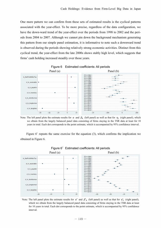
One more pattern we can confirm from these sets of estimated results is the cyclical patterns associated with the year-effect. To be more precise, regardless of the data configuration, we have the down-ward trend of the year-effect over the periods from 1998 to 2002 and the peri-ods from 2004 to 2007. Although we cannot pin down the background mechanism generating this pattern from our simple panel estimation, it is informative to note such a downward trend is observed during the periods showing relatively strong economic activities. Distinct from this cyclical trend, the year-effect from the late 2000s shows stably high level, which suggests that firms’ cash holding increased steadily over those years.
Figure 6 Estimated coefficients: All periods
Panel (a) Panel (b)
Note: The left panel plots the estimate results for � and �� (left panel) as well as that for �� (right panel), which
we obtain from the largely balanced panel data consisting of firms staying in the TSR data at least for 10 years in total. Each dot corresponds to the point estimate, which is accompanied by 95% confidence interval.
Figure 6’ repeats the same exercise for the equation (3), which confirms the implication we
obtained in Figure 6.
Figure 6′Estimated coefficients: All periods Panel (a) Panel (b)
Note: The left panel plots the estimate results for �� and ��� (left panel) as well as that for ��� (right panel),
which we obtain from the largely balanced panel data consisting of firms staying in the TSR data at least for 10 years in total. Each dot corresponds to the point estimate, which is accompanied by 95% confidence interval.
『経済分析』第 200 号
148
year-specific effect, for example, in the year of 2009 (i.e., the accounting periods ending on June of the year 2009 and the May of the year 2010) followed by the relatively higher levels of year-effect than for the periods up to the late 2000s. This observation again allows us to confirm the recent trend of firms’ increasing cash holdings.
Figure 5’ repeats the same exercise for the equation (3). First, we can confirm the re-sponse of the level of cash holding to each independent variable is qualitatively same as we reported in Figure 5. One thing we can notice from Figure 5’ is that now the positive coeffi-cient associated with the cash inflow (i.e., ln_NetProditAfterTax) is the largest among the other items associated with positive coefficients. Given the standard deviation of the cash inflow is larger than that for other independent variables (See Table 1), we can confirm that the cash in-flow is the one most largely driving the level of firms’ cash holding. Second, as we found in Figure 4, Panel (b) of Figure 5’ shows the clear dynamics of the year-effect.
Figure 5′Estimated coefficients: All periods
Panel (a) Panel (b)
Note: The left panel plots the estimate results for �� and ��� (left panel) as well as that for ��� (right panel),
which we obtain from the estimation using all the TSR data. Each dot corresponds to the point estimate, which is accompanied by 95% confidence interval.
How does the change in data configuration affect the abovementioned results? Figure 6 and Figure 7 repeat the same firm-level panel estimation for ������������� by using the
largely balanced panel data consisting of firms staying in the TSR data at least for 10 years in total (Figure 6) and the balanced panel data constructed over the sample periods (Figure 7). We can immediately confirm that the association between ������������� and the right
hand-side variables are in the same pattern as we observed in Figure 5. Thanks to the large number of observation stored in our datasets, the confidence band is narrow enough to be con-fident about the statistical significance of those estimated coefficients even in the case of bal-anced panel estimation. We can also confirm the same pattern for the year-effect as in Figure 5.
- 148 - - 149 -

『経済分析』第 200 号
150
Figure 7 Estimated coefficients: All periods
Panel (a) Panel (b)
Note: The left panel plots the estimate results for � and �� (left panel) as well as that for �� (right panel), which
we obtain from the balanced panel data constructed over the sample periods. Each dot corresponds to the point estimate, which is accompanied by 95% confidence interval.
Figure 7’ repeats the same exercise for the equation (3), which confirms the implication we
obtained in Figure 7.
Figure 7′Estimated coefficients: All periods
Panel (a) Panel (b)
Note: The left panel plots the estimate results for �� and ��� (left panel) as well as that for ��� (right panel),
which we obtain from the balanced panel data constructed over the sample periods. Each dot corresponds to the point estimate, which is accompanied by 95% confidence interval.
Given these natural results reported in the previous subsection, it is informative to see how these associations have been evolving over the sample periods. If we find greater associa-tion between the cash holdings and specific variables, we can infer that the main sources for accumulating cash have been changing over the last two decades. In order to explicitly see the evolution of the estimated coefficients over the periods from 1994 to 2016, we split the periods
- 150 -
Cash Holdings: Evidence from Firm-Level Big Data in Japan
151
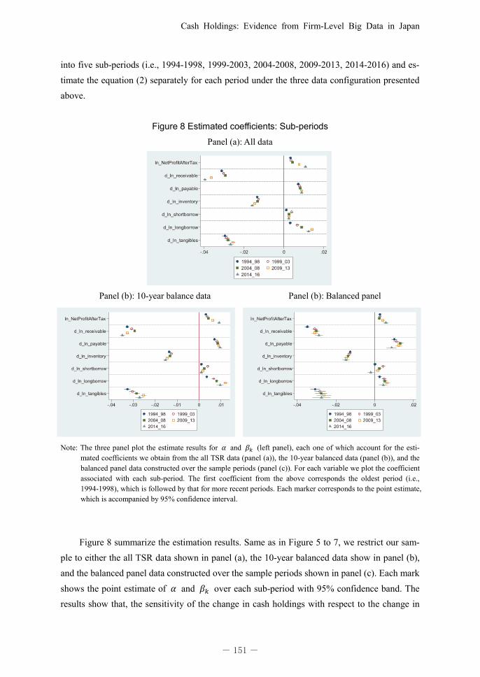
into five sub-periods (i.e., 1994-1998, 1999-2003, 2004-2008, 2009-2013, 2014-2016) and es-timate the equation (2) separately for each period under the three data configuration presented above.
Figure 8 Estimated coefficients: Sub-periods
Panel (a): All data
Panel (b): 10-year balance data Panel (b): Balanced panel
Note: The three panel plot the estimate results for and (left panel), each one of which account for the esti-
mated coefficients we obtain from the all TSR data (panel (a)), the 10-year balanced data (panel (b)), and the balanced panel data constructed over the sample periods (panel (c)). For each variable we plot the coefficient associated with each sub-period. The first coefficient from the above corresponds the oldest period (i.e., 1994-1998), which is followed by that for more recent periods. Each marker corresponds to the point estimate, which is accompanied by 95% confidence interval.
Figure 8 summarize the estimation results. Same as in Figure 5 to 7, we restrict our sam-ple to either the all TSR data shown in panel (a), the 10-year balanced data show in panel (b), and the balanced panel data constructed over the sample periods shown in panel (c). Each mark shows the point estimate of and over each sub-period with 95% confidence band. The results show that, the sensitivity of the change in cash holdings with respect to the change in
『経済分析』第 200 号
150
Figure 7 Estimated coefficients: All periods
Panel (a) Panel (b)
Note: The left panel plots the estimate results for � and �� (left panel) as well as that for �� (right panel), which
we obtain from the balanced panel data constructed over the sample periods. Each dot corresponds to the point estimate, which is accompanied by 95% confidence interval.
Figure 7’ repeats the same exercise for the equation (3), which confirms the implication we
obtained in Figure 7.
Figure 7′Estimated coefficients: All periods
Panel (a) Panel (b)
Note: The left panel plots the estimate results for �� and ��� (left panel) as well as that for ��� (right panel),
which we obtain from the balanced panel data constructed over the sample periods. Each dot corresponds to the point estimate, which is accompanied by 95% confidence interval.
Given these natural results reported in the previous subsection, it is informative to see how these associations have been evolving over the sample periods. If we find greater associa-tion between the cash holdings and specific variables, we can infer that the main sources for accumulating cash have been changing over the last two decades. In order to explicitly see the evolution of the estimated coefficients over the periods from 1994 to 2016, we split the periods
- 150 - - 151 -
『経済分析』第 200 号
152
cash inflow (i.e., ) becomes substantially larger since the late 2000s.2 This implies that bet-ter performed firms are more likely to accumulate cash, which leads to wider dispersion of cash holding among firms. This tendency becomes more apparent once we include new entrant firms to our analysis (i.e., panel (a) and (b)).
Interestingly, from the panel (a) and (b) where the data include newly entrant firms and exiting firms, larger long-term borrowing and smaller account receivables in addition to the abovementioned larger cash inflow also contribute to higher cash holding over the recent peri-ods. We can also find that, in panel (a) and (b), the change in tangibles become less important to the change in cash holdings over the recent periods. Thus, we can presume that well-performed firms tend to accumulate their cash by taking advantage of better business (higher cash inflow) and financing conditions (larger long-term borrowing and smaller account receivables). This also means that firms with worse performance actually show the decline in cash holding. We should note that such a polarization of firms in terms of cash holding emerged at the same time as the average increasing trend in cash holdings.
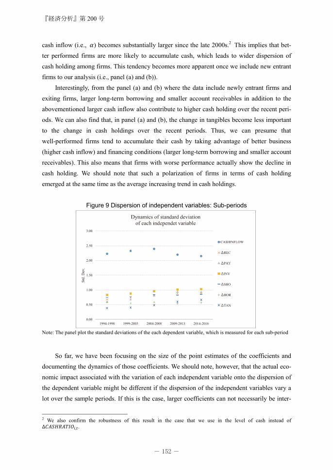
Figure 9 Dispersion of independent variables: Sub-periods
Note: The panel plot the standard deviations of the each dependent variable, which is measured for each sub-period
So far, we have been focusing on the size of the point estimates of the coefficients and
documenting the dynamics of those coefficients. We should note, however, that the actual eco-nomic impact associated with the variation of each independent variable onto the dispersion of the dependent variable might be different if the dispersion of the independent variables vary a lot over the sample periods. If this is the case, larger coefficients can not necessarily be inter-
2 We also confirm the robustness of this result in the case that we use in the level of cash instead of
.
- 152 -

Cash Holdings: Evidence from Firm-Level Big Data in Japan
153
preted as in the way we explained above. Given this concern, Figure 9 depict the dynamics of the standard deviation of the independent variables we use for the equations (2) and (3). What we can observe from this figure is, first, the small change in the dispersion of the cash inflow. Second, we can also find the increase in the dispersion of the variables accounting for the trade credit variables. The point estimates we reported have already implied the possibility that well-performed firms tend to accumulate their cash more by taking advantage of higher cash inflow and financing conditions. These two facts observed in Figure 9 further suggest that those implication are robust in terms of economic impacts as the product of coefficient and the dispersion become larger for the cash inflow and trade credit varaibles. We will provide more detailed discussion for this issue in the latter section again.
3.4 Conditional effect of cash inflow
Given that the hike in the positive coefficient associated with ������������� is one
salient feature over the recent years, it would be further informative to see under what situation such a positive impact running from ������������� to ������������� becomes more
apprent. This discussion would allow us to more precisely understand the mechanism govern-ing the polarization of cash holdings. For this purpose, we estimate the following equation (4) which augments the equation (2) with the level of each balance sheet variables ������� as of t-1 as well as its interaction term with �������������. We are specifically interested in the co-
efficients �� , which are associated with the interaction terms between ������� and ������������� . The set of these coefficients �� summarize the impact of
������������� conditional on the level of ������� .
������������� � �������������� � ∑ ������������
�∑ ������������� � ������������� � ∑ ������������� � �� � �� � ���� (4)
Figure 10 plots the point estimates of � and �� in the left panel and set of �� in the right panel. First, we can observe that the ������������� shows substantially higher asso-ciation with ������������� over the recent periods (i.e., 2009-2013 and 2014-2016). Sec-ond, we can see such a positive impact of ������������� is conditional on the level of oth-
er balance sheet items (i.e., ������� ). Namely, smaller account receivables, larger account paya-bles, smaller inventory, larger long-term borrowing, and smaller tangible assets as of t-1 lead to substantially larger marginal effect running from ������������� to �������������. To
illustrate, the results associated with the account receivables, inventory, and account payables imply that firms with smaller working capital demand can more easily convert their cash in-flow to their cash holdings. Given the discussions in the extant studies, which consider the fi-
『経済分析』第 200 号
152
cash inflow (i.e., ) becomes substantially larger since the late 2000s.2 This implies that bet-ter performed firms are more likely to accumulate cash, which leads to wider dispersion of cash holding among firms. This tendency becomes more apparent once we include new entrant firms to our analysis (i.e., panel (a) and (b)).
Interestingly, from the panel (a) and (b) where the data include newly entrant firms and exiting firms, larger long-term borrowing and smaller account receivables in addition to the abovementioned larger cash inflow also contribute to higher cash holding over the recent peri-ods. We can also find that, in panel (a) and (b), the change in tangibles become less important to the change in cash holdings over the recent periods. Thus, we can presume that well-performed firms tend to accumulate their cash by taking advantage of better business (higher cash inflow) and financing conditions (larger long-term borrowing and smaller account receivables). This also means that firms with worse performance actually show the decline in cash holding. We should note that such a polarization of firms in terms of cash holding emerged at the same time as the average increasing trend in cash holdings.
Figure 9 Dispersion of independent variables: Sub-periods
Note: The panel plot the standard deviations of the each dependent variable, which is measured for each sub-period
So far, we have been focusing on the size of the point estimates of the coefficients and
documenting the dynamics of those coefficients. We should note, however, that the actual eco-nomic impact associated with the variation of each independent variable onto the dispersion of the dependent variable might be different if the dispersion of the independent variables vary a lot over the sample periods. If this is the case, larger coefficients can not necessarily be inter-
2 We also confirm the robustness of this result in the case that we use in the level of cash instead of
.
- 152 - - 153 -

『経済分析』第 200 号
154
nancial friction as the main determinant of cash holding, this result is in fact surprising. Ac-cording to a theoretical discussion, firms with smaller need for finance (i.e.,, smaller working capital in the current context) does not need to secure larger cash, which is not the case here.
Figure 10 Estimated coefficients: Sub-periods and interaction term (all data)
Note: The three panel plot the estimate results for and (left panel) as well as (right panel), each one of
which account for the estimated coefficients we obtain from the all TSR data. For each variable we plot the coefficient associated with each sub-period. The first coefficient from the above corresponds the oldest period (i.e., 1994-1998), which is followed by that for more recent periods. Each dot corresponds to the point esti-mate, which is accompanied by 95% confidence interval.
We should also note that such a pattern becomes more apparent over the recent periods.
This result reassures the findings we have already reported, i.e., firms with better financial po-sition actually accumulate their cash holdings. Related to this point, another interesting pattern could be found for the coefficient associated with the interaction term between cash inflow in year t and the long-term borrowing as of year t-1. Larger positive coefficient of this interaction term means that firms with larger long-term borrowing tend to convert more cash inflow to cash holdings. Such a larger sensitivity of cash holdings with respect to cash inflow in the case of more levered firms could be the case, for example, when firms are facing larger uncertainty and, thus would largely like to accumulate cash if they can. Our result also suggests that firms are more likely to accumulate cash when facing more relaxed borrowing condition.
The coefficient associated with the interaction term between cash inflow in year t and the tangible assets as of year t-1 shows negative sign. This implies that firms with more tangible assets and thus need to implement a certain level of capital investment could not largely con-vert its cash inflow to cash holdings.
Figure 11 and 12 check the robustness of the results we observed in Figure 10 by using the two other data configurations. Presumably due to the reduction of sample size, the confidence band becomes larger but the estimated with the coefficient associated with the interaction term between cash inflow in year t and the account payable and inventory as of year t-1 shows the
- 154 -

Cash Holdings: Evidence from Firm-Level Big Data in Japan
155
same implication as we reported.
Figure 11 Estimated coefficients: Sub-periods and interaction term (10-year balanced)
Note: The three panel plot the estimate results for and (left panel) as well as (right panel), each one of
which account for the estimated coefficients we obtain from the 10-year balanced data. For each variable we plot the coefficient associated with each sub-period. The first coefficient from the above corresponds the old-est period (i.e., 1994-1998), which is followed by that for more recent periods. Each dot corresponds to the point estimate, which is accompanied by 95% confidence interval.
Figure 12 Estimated coefficients: Sub-periods and interaction term (balanced)
Note: The three panel plot the estimate results for and (left panel) as well as (right panel), each one of
which account for the estimated coefficients we obtain from the balanced panel data. For each variable we plot the coefficient associated with each sub-period. The first coefficient from the above corresponds the old-est period (i.e., 1994-1998), which is followed by that for more recent periods. Each dot corresponds to the point estimate, which is accompanied by 95% confidence interval.
As we have already pointed out, in order to precisely interpret the economic impacts as-sociated with the estimated coefficients, we need to take into account the dynamics of standard deviation associated with each independent variable. For this purpose, we did the following exercise. First, we computed the standard deviation of all the variables in the right hand-side of the equation (4). Second, we computed the predicted change in the dependent variable (i.e.,
『経済分析』第 200 号
154
nancial friction as the main determinant of cash holding, this result is in fact surprising. Ac-cording to a theoretical discussion, firms with smaller need for finance (i.e.,, smaller working capital in the current context) does not need to secure larger cash, which is not the case here.
Figure 10 Estimated coefficients: Sub-periods and interaction term (all data)
Note: The three panel plot the estimate results for and (left panel) as well as (right panel), each one of
which account for the estimated coefficients we obtain from the all TSR data. For each variable we plot the coefficient associated with each sub-period. The first coefficient from the above corresponds the oldest period (i.e., 1994-1998), which is followed by that for more recent periods. Each dot corresponds to the point esti-mate, which is accompanied by 95% confidence interval.
We should also note that such a pattern becomes more apparent over the recent periods.
This result reassures the findings we have already reported, i.e., firms with better financial po-sition actually accumulate their cash holdings. Related to this point, another interesting pattern could be found for the coefficient associated with the interaction term between cash inflow in year t and the long-term borrowing as of year t-1. Larger positive coefficient of this interaction term means that firms with larger long-term borrowing tend to convert more cash inflow to cash holdings. Such a larger sensitivity of cash holdings with respect to cash inflow in the case of more levered firms could be the case, for example, when firms are facing larger uncertainty and, thus would largely like to accumulate cash if they can. Our result also suggests that firms are more likely to accumulate cash when facing more relaxed borrowing condition.
The coefficient associated with the interaction term between cash inflow in year t and the tangible assets as of year t-1 shows negative sign. This implies that firms with more tangible assets and thus need to implement a certain level of capital investment could not largely con-vert its cash inflow to cash holdings.
Figure 11 and 12 check the robustness of the results we observed in Figure 10 by using the two other data configurations. Presumably due to the reduction of sample size, the confidence band becomes larger but the estimated with the coefficient associated with the interaction term between cash inflow in year t and the account payable and inventory as of year t-1 shows the
- 154 - - 155 -
『経済分析』第 200 号
156
) by multiplying such standard deviation to the estimated coefficient including the cross-terms so that we can see the change in generated by one standard deviation change in each right hand-side variable. Third, we compute the contribution associ-ated with the one standard deviation change in each independent variable as a share to one standard deviation of . This share accounts for how much of the change in
could be accounted for by the change in each independent variable. As we have already confirmed, each independent variable has either positive or negative coefficient, which shows the increase in a specific independent variable leads to either larger or smaller
. For the purpose of presentation, we measure the absolute value of the products between the standard deviation and the estimated coefficient, then sum up the contributions of trade credit-related variables and inventory (i.e., “Trade credit & Inventory”). Also, the short-term and long-term borrowing are summarized in one category (i.e., “Borrowing”). Those numbers are summarized in Figure 13 where the solid line accounts for the dynamics of the product between the estimated coefficient associated with and the standard deviation of
. The other three dashed lines accounts for that of the three interaction terms (i.e., with “Trade credit & Inventory” variable, “Borrowing” variables, and tangibles) over each sub-period.
Figure 13 suggests, first, that the contribution associated with has been
becoming the largest in the most recent period (i.e., 2014-2016). Also, the contribution shows a clear upward trend from the period of 2009-2013. In terms of the economic impact, the solid line suggests that the one standard deviation increase in accounts for around 60% of the one standard deviation change in in the period 2014-2016.
Second, we can further confirm that the contribution originated from the interaction term between and “Trade credit & Inventory” variables show the similar pattern and sizable impact. To interpret the results precisely, we should note that both the interaction terms between with account receivables and inventory have negative coeffi-cients while the interaction term between with account payable has a positive coefficient. Thus, the sum of the absolute values of the products between the standard devia-tions and the estimated coefficients, which is denoted by “Trade credit & Inventory” (dashed line with black circle), accounts for how much percentage of one standard deviation of
could be explained by the one standard deviation decrease in account receiva-bles and inventory as well as the one standard deviation increase in account payable each cat-egory when those change are accompanied by the one standard deviation change in
. The results in Figure 13 denoted by “Trade credit & Inventory” suggests that, if those “Trade credit & Inventory” change by one standard deviation in the favor direction of larger , the one standard deviation increase in accounts for
- 156 -

Cash Holdings: Evidence from Firm-Level Big Data in Japan
157
around 15% of the one standard deviation change in . By construction, this 15% is added up to the abovementioned unconditional contribution of (i.e., 60% of the one standard deviation change in ). These exercise tells us that the interpretation of the estimated coefficients are confirmed in terms of the economic impacts.
Figure13 Decomposition of the dispersion of cash holding (all data)
Note: The panel depict the dynamics of the multiplication between the estimated coefficient associated with a spe-
cific (or a group of) independent variable(s) and the standard deviation of the variable(s). The solid line ac-counts for the dynamics of the multiplication between the estimated coefficient associated with and the standard deviation of . The other three dashed lines accounts for that of the three interaction terms (i.e., with “Trade credit & Inventory” variable, “Borrow-ing” variables, and tangibles) over each sub-period.
3.5 Heterogeneity in transaction relations Figure 2 and 3 presented in the previous section suggest that while firms’ cash holding on
average show the increasing trend over the recent periods, there is still a substantial degree of firm-level heterogeneity represented by firms’ balance sheet conditions. In particular, it is an important finding that the status of trade finance (i.e., the level of account receivables and ac-count payables) affect the marginal impact of cash inflow onto cash holdings more in the re-cent periods. Regardless of whether we focus on the statistical significance or economic im-pacts, we confirm that larger leads to higher and this ten-dency becomes more apparent when firms are facing smaller demand for working capital (i.e., smaller account receivables and inventory as well as larger account payables).
These results are not consistent with firms’ precautionary saving motive as firms in better position in trade credit tend to accumulate more cash. Following this context, in this section, we would revisit firms’ precautionary motives with respect to real transaction with customers and suppliers. We presume that, if well-performed firms are transacting with a larger number
『経済分析』第 200 号
156
) by multiplying such standard deviation to the estimated coefficient including the cross-terms so that we can see the change in generated by one standard deviation change in each right hand-side variable. Third, we compute the contribution associ-ated with the one standard deviation change in each independent variable as a share to one standard deviation of . This share accounts for how much of the change in
could be accounted for by the change in each independent variable. As we have already confirmed, each independent variable has either positive or negative coefficient, which shows the increase in a specific independent variable leads to either larger or smaller
. For the purpose of presentation, we measure the absolute value of the products between the standard deviation and the estimated coefficient, then sum up the contributions of trade credit-related variables and inventory (i.e., “Trade credit & Inventory”). Also, the short-term and long-term borrowing are summarized in one category (i.e., “Borrowing”). Those numbers are summarized in Figure 13 where the solid line accounts for the dynamics of the product between the estimated coefficient associated with and the standard deviation of
. The other three dashed lines accounts for that of the three interaction terms (i.e., with “Trade credit & Inventory” variable, “Borrowing” variables, and tangibles) over each sub-period.
Figure 13 suggests, first, that the contribution associated with has been
becoming the largest in the most recent period (i.e., 2014-2016). Also, the contribution shows a clear upward trend from the period of 2009-2013. In terms of the economic impact, the solid line suggests that the one standard deviation increase in accounts for around 60% of the one standard deviation change in in the period 2014-2016.
Second, we can further confirm that the contribution originated from the interaction term between and “Trade credit & Inventory” variables show the similar pattern and sizable impact. To interpret the results precisely, we should note that both the interaction terms between with account receivables and inventory have negative coeffi-cients while the interaction term between with account payable has a positive coefficient. Thus, the sum of the absolute values of the products between the standard devia-tions and the estimated coefficients, which is denoted by “Trade credit & Inventory” (dashed line with black circle), accounts for how much percentage of one standard deviation of
could be explained by the one standard deviation decrease in account receiva-bles and inventory as well as the one standard deviation increase in account payable each cat-egory when those change are accompanied by the one standard deviation change in
. The results in Figure 13 denoted by “Trade credit & Inventory” suggests that, if those “Trade credit & Inventory” change by one standard deviation in the favor direction of larger , the one standard deviation increase in accounts for
- 156 - - 157 -

『経済分析』第 200 号
158
of customers, there is smaller need for the firms to secure cash for the purpose of payment as the default risk associated each customer is well diversified. In a similar sense, if well-performed firms are transacting with a larger number of suppliers, there is smaller need for the firms to secure cash for the purpose of payment as the risk of product disruption associ-ated each supplier is well diversified. Thus, such firms can pay out larger amount of cash in-flow for various purposes (e.g., investment, dividend, repayment of debt etc.) and result in moderate cash holdings. On the other hand, even if firms with high profit, they might not pay out the cash if worried about their trade relations.
To test this intuition more explicitly, we run the following cross-sectional regression of the equation (5) where ���������� accounts for the cash-to-total asset ratio of firm i as of 2014 while the cash inflow we featured in the previous study is proxied for by ��������������������� , the dummy variable taking value of one if pre-tax net prof-it-to-sales ratio is greater than sample median. To measure the heterogeneity of trade relations, we measure the number of customers and suppliers (������ and ������). In this regres-sion, we expect �� � � as we confirmed in the previous section while �� � � and �� � � based on the abovementioned presumption.
In order to control for various firm attributes potentially confounding the ��, ��, and ��,
we control for the following variables ��� consisting of the natural logarithm of sales in year t-1, the sales grows from year t-2 to t-1, the dummy variable taking value of one if firm exhib-its loss in year t-1, the difference of such loss dummy from t-2 to t-1, the natural logarithm of the number of employees in year t-1, firm age, the dummy variable taking value of one if firm owns a single establishment, the dummy variable taking value of one if firm is listed, the natu-ral logarithm of total assets in year t-1, tangible assets total assets ratio in year t-1, liability to total assets ratio in year t-1, bank borrowing to total assets ratio in year t-1, fixed assets to eq-uity ratio in year t-1, the natural logarithm of EBITDA in year t-1, the dummy variable taking value of one if firm experienced default prior to year t, the number of lender banks, and the dummy variable taking value of one if firm changed its main bank from year t-1 to t, and the industry dummy variables accounting for two-digit industry classification.
���������� � �� � ����������������������� ��������� � ����������������������� � ������
��������������� � ����������������������� � ������ � ∑ ��������� � �� (5) Figure 14 shows the estimated conditional slope with respect to the high profit-to-sales
ratio dummy conditional on ������ and ������.3 As we predicted, firms with higher cash
3 Given the non-linearity of the model, the estimated conditional slope shows some curves.
- 158 -
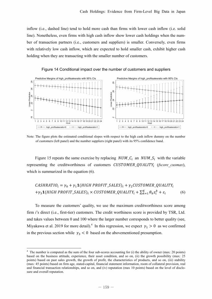
Cash Holdings: Evidence from Firm-Level Big Data in Japan
159
inflow (i.e., dashed line) tend to hold more cash than firms with lower cash inflow (i.e. solid line). Nonetheless, even firms with high cash inflow show lower cash holdings when the num-ber of transaction partners (i.e., customers and suppliers) is smaller. Conversely, even firms with relatively low cash inflow, which are expected to hold smaller cash, exhibit higher cash holding when they are transacting with the smaller number of customers.
Figure 14 Conditional impact over the number of customers and suppliers
Note: The figure plots the estimated conditional slopes with respect to the high cash inflow dummy on the number
of customers (left panel) and the number suppliers (right panel) with its 95% confidence band.
Figure 15 repeats the same exercise by replacing ������ an ������ with the variable
representing the creditworthiness of customers ����������������� (fscore_cusmax), which is summarized in the equation (6).
���������� � �� � ����������������������� � �������������������
������������������������ � ����������������� � ∑ ��������� � �� (6) To measure the customers’ quality, we use the maximum creditworthiness score among
firm i’s direct (i.e., first-tier) customers. The credit worthiness score is provided by TSR, Ltd. and takes values between 0 and 100 where the larger number corresponds to better quality (see, Miyakawa et al. 2019 for more detail).4 In this regression, we expect �� � � as we confirmed in the previous section while �� � � based on the abovementioned presumption.
4 The number is computed as the sum of the four sub-scores accounting for (i) the ability of owner (max: 20 points) based on the business attitude, experience, their asset condition, and so on, (ii) the growth possibility (max: 25 points) based on past sales growth, the growth of profit, the characteristics of products, and so on, (iii) stability (max: 45 points) based on firm age, stated-capital, financial statement information, room of collateral provision, real and financial transaction relationships, and so on, and (iv) reputation (max 10 points) based on the level of disclo-sure and overall reputation.
.18
.2.2
2.2
4.2
6.2
8Li
near
Pre
dict
ion
1 2 3 4 5 6 7 8 9 10 11 12 13 14 15 16 17 18 19 20 21 22 23 24ncus
high_profitsalesratio=0 high_profitsalesratio=1
Predictive Margins of high_profitsalesratio with 95% CIs
.2.2
2.2
4.2
6.2
8Li
near
Pre
dict
ion
1 2 3 4 5 6 7 8 9 10 11 12 13 14 15 16 17 18 19 20 21 22 23 24nsup
high_profitsalesratio=0 high_profitsalesratio=1
Predictive Margins of high_profitsalesratio with 95% CIs
『経済分析』第 200 号
158
of customers, there is smaller need for the firms to secure cash for the purpose of payment as the default risk associated each customer is well diversified. In a similar sense, if well-performed firms are transacting with a larger number of suppliers, there is smaller need for the firms to secure cash for the purpose of payment as the risk of product disruption associ-ated each supplier is well diversified. Thus, such firms can pay out larger amount of cash in-flow for various purposes (e.g., investment, dividend, repayment of debt etc.) and result in moderate cash holdings. On the other hand, even if firms with high profit, they might not pay out the cash if worried about their trade relations.
To test this intuition more explicitly, we run the following cross-sectional regression of the equation (5) where ���������� accounts for the cash-to-total asset ratio of firm i as of 2014 while the cash inflow we featured in the previous study is proxied for by ��������������������� , the dummy variable taking value of one if pre-tax net prof-it-to-sales ratio is greater than sample median. To measure the heterogeneity of trade relations, we measure the number of customers and suppliers (������ and ������). In this regres-sion, we expect �� � � as we confirmed in the previous section while �� � � and �� � � based on the abovementioned presumption.
In order to control for various firm attributes potentially confounding the ��, ��, and ��,
we control for the following variables ��� consisting of the natural logarithm of sales in year t-1, the sales grows from year t-2 to t-1, the dummy variable taking value of one if firm exhib-its loss in year t-1, the difference of such loss dummy from t-2 to t-1, the natural logarithm of the number of employees in year t-1, firm age, the dummy variable taking value of one if firm owns a single establishment, the dummy variable taking value of one if firm is listed, the natu-ral logarithm of total assets in year t-1, tangible assets total assets ratio in year t-1, liability to total assets ratio in year t-1, bank borrowing to total assets ratio in year t-1, fixed assets to eq-uity ratio in year t-1, the natural logarithm of EBITDA in year t-1, the dummy variable taking value of one if firm experienced default prior to year t, the number of lender banks, and the dummy variable taking value of one if firm changed its main bank from year t-1 to t, and the industry dummy variables accounting for two-digit industry classification.
���������� � �� � ����������������������� ��������� � ����������������������� � ������
��������������� � ����������������������� � ������ � ∑ ��������� � �� (5) Figure 14 shows the estimated conditional slope with respect to the high profit-to-sales
ratio dummy conditional on ������ and ������.3 As we predicted, firms with higher cash
3 Given the non-linearity of the model, the estimated conditional slope shows some curves.
- 158 - - 159 -

『経済分析』第 200 号
160
Figure 15 Conditional impact over the creditworthiness of customers
Note: The figure plots the estimated conditional slopes with respect to the high cash inflow dummy on the maxi-
mum credit worthiness score (i.e., fscore) with its 95% confidence band.
Figure 15 shows the estimated slope with respect to the high profit-to-sales ratio dummy
conditional on (fscore_cusmax). As we predicted, firms with higher cash inflow (i.e., dashed line) tend to hold more cash than firms with lower cash inflow (i.e. solid line). Nonetheless, even firms with high cash inflow show lower cash holdings when the quality of their customers is higher (i.e., higher fscore_cusmax). Conversely, even firms with relatively low cash inflow, which are expected to hold smaller cash, exhibit higher cash hold-ing when they are transacting with lower quality customers. 3.6 Policy implication
Throughout this section, we have documented the firm-level heterogeneity in terms of their balance sheet as well as attributes of firms’ transaction partners. These descriptive anal-yses provide us at least three policy implications.
First, the substantial role of firm-level heterogeneity especially in regard of cash inflow and the status of firm-to-firm transaction (i.e., trade credit and trader partners’ quality) suggest the importance of micro-level empirical analysis in the policy discussion. While a simple illus-tration provided in, for example, Figure 2 could suggest the fact that the increase in the first moment of the cash holding is also accompanied by the increase in the cross-sectional disper-sion of cash holding, we have not seen specific policy discussions paying an attention to this point. It is fair to alert that policy discussion not based on valid empirical analysis could mis-lead the policy design. In this context, it is also meaningful to highlight the abovementioned fact from an opposite angle. Namely, higher sensitivity of cash holding with respect to cash inflow suggests firms with lower cash inflow cannot secure their cash holding. This is one of the empirical facts policy makers may take into account. We should remember that this fact is
.2.2
5.3
.35
.4.4
5Li
near
Pre
dict
ion
16 26 36 46 56 66 76 86fscore_cusmax
high_profitsalesratio=0 high_profitsalesratio=1
Adjusted Predictions of high_profitsalesratio with 95% CIs
- 160 -
Cash Holdings: Evidence from Firm-Level Big Data in Japan
161
obtained under the model with year-fixed effects, which presumably account for various ag-gregate-level shock. Even if we can successfully take care of negative aggregate shock such as financial crisis through some policy measures, our findings still suggest a room of taking care of the firms with smaller buffer for their cash position.
Second, among those important firm-level heterogeneities, the fact that firms with larger cash inflow are accumulating larger size of cash over the recent period, which is more apparent when firms do not need larger working capital, is suggestive. Standard theory of precautionary saving suggest that firms hold cash with some sort of anxiety for future finance, which moti-vates them to save more. From the fact that even seemingly well-performing firms in a better financial position are accumulating cash, we might better to presume that micro-level uncer-tainty as well as the aggregate-level factors we highlighted in, for example, Figure 4, play sub-stantial role in the context of firm’s saving behavior. Although it is beyond the scope of this paper, digging into those firm-level uncertainty (e.g., Senga 2018) would one promising direc-tion future research should pursue.
Third, apart from the discussion on firm-level uncertainty, our findings still suggest that precautionary saving motive matters, which is confirmed through the analyses highlighting the role of transaction network in terms of firms’ cash holding. Given a large accumulation of firm-to-firm transaction network data such as the one provided by Tokyo Shoko Research (TSR), Ltd. (see, for example Miyakawa 2019), it would be a promising direction to see the relationship between the network structure and firms’ cash holding behavior. If firms are facing more secure transaction network, which could be achieved by, for example, payment system governed by highly sophisticated system such as blockchain, firms might not need to hold a large amount of cash in their hand. The recent discussion on ICT and other technological issues are in this sense well connected to the main theme of the present paper.
4.Conclusion
In the present paper, to investigate the status of firms’ cash holdings, first, we document how the distribution of firms’ cash holding has been evolving over the last two decades. Our descriptive analyses suggest that since the late 2000s, firms on average have increased its size-adjusted cash holding. This trend has been also accompanied by increasing dispersion of cash holding among firms, which suggests the presence of firm-level heterogeneity behind the recent trend of larger cash holdings. Second, we document how firms have increased their cash holdings. The results of our panel estimation show that the sensitivity of the change in cash holdings with respect to the change in cash inflow becomes substantially larger since the late
『経済分析』第 200 号
160
Figure 15 Conditional impact over the creditworthiness of customers
Note: The figure plots the estimated conditional slopes with respect to the high cash inflow dummy on the maxi-
mum credit worthiness score (i.e., fscore) with its 95% confidence band.
Figure 15 shows the estimated slope with respect to the high profit-to-sales ratio dummy
conditional on (fscore_cusmax). As we predicted, firms with higher cash inflow (i.e., dashed line) tend to hold more cash than firms with lower cash inflow (i.e. solid line). Nonetheless, even firms with high cash inflow show lower cash holdings when the quality of their customers is higher (i.e., higher fscore_cusmax). Conversely, even firms with relatively low cash inflow, which are expected to hold smaller cash, exhibit higher cash hold-ing when they are transacting with lower quality customers. 3.6 Policy implication
Throughout this section, we have documented the firm-level heterogeneity in terms of their balance sheet as well as attributes of firms’ transaction partners. These descriptive anal-yses provide us at least three policy implications.
First, the substantial role of firm-level heterogeneity especially in regard of cash inflow and the status of firm-to-firm transaction (i.e., trade credit and trader partners’ quality) suggest the importance of micro-level empirical analysis in the policy discussion. While a simple illus-tration provided in, for example, Figure 2 could suggest the fact that the increase in the first moment of the cash holding is also accompanied by the increase in the cross-sectional disper-sion of cash holding, we have not seen specific policy discussions paying an attention to this point. It is fair to alert that policy discussion not based on valid empirical analysis could mis-lead the policy design. In this context, it is also meaningful to highlight the abovementioned fact from an opposite angle. Namely, higher sensitivity of cash holding with respect to cash inflow suggests firms with lower cash inflow cannot secure their cash holding. This is one of the empirical facts policy makers may take into account. We should remember that this fact is
.2.2
5.3
.35
.4.4
5Li
near
Pre
dict
ion
16 26 36 46 56 66 76 86fscore_cusmax
high_profitsalesratio=0 high_profitsalesratio=1
Adjusted Predictions of high_profitsalesratio with 95% CIs
- 160 - - 161 -
『経済分析』第 200 号
162
2000s. This implies that better-performed firms have become more likely to accumulate cash. Given the results from this unconditional estimation, we further take into account firm-level heterogeneity in terms of their balance sheet conditions and found that firms holding smaller account receivables and/or inventory tend to show further higher sensitivity. This implies that firms with smaller working capital needs can save more cash, which is somewhat surprising given the extant studies considering financial friction as the key determinants of cash holding. We also confirm that firms with smaller number of customer typically show such a higher sen-sitivity.
These results we present in the present paper jointly suggest that firms’ recent tendency to hold larger cash is driven by a combination of larger cash inflow and firms’ various motiva-tions. On the one hand, well-performing firms with better business conditions and financial positions are more likely to accumulate cash. On the other hand, firms having precautionary saving motive have been also accumulating cash. These heterogeneous motivations for firms to hold cash need to be simultaneously considered to understand firms’ cash holding behavior more precisely.
Reference
Almeida, H., M. Campello, and M. Weisbach (2004), “The Cash Flow Sensitivity of Cash,” Journal of Finance, 59(4), pp. 1777-1804.
Bates, T.W., K.M.Kahle, and R.M. Stultz (2009), “Why Do US Firms Hold So Much More Cash than They Used to Be?” Journal of Finance, 64(5), pp. 1985-2021.
Denis, D.J. and V. Sibilkov (2009), “Financial Constraints, Investment and the Value of Cash Holdings,” Review of Financial Studies, 23(1), pp. 247-269.
Graham, J. R. and M. T. Leary (2018), “The Evolution of Corporate Cash,” Review of Finan-cial Studies, 31(11), pp. 4288-4344.
Harford, J., S. Klasa, and W.F. Maxwell (2014), “Refinancing Risk and Cash Holdings,” Jour-nal of Finance, 69(3), pp. 975-1012.
Hosono, K., D. Miyakawa, M. Takizawa, and K, Yamanouchi (2016), “Complementarity and Substitutability between Tangible and Intangible Capital: Evidence from Japanese Firm-level Data,” RIETI Discussion Paper 16-E-024.
Hosono, K., D. Miyakawa, and M. Takizawa (2017), “Intangible Assets and Firms’ Liquidity Holdings: Evidence from Japan,” RIETI Discussion Paper 17-E-053.
Jensen, M. (1986), “Agency Costs of Free Cash Flow, Corporate Finance and Takeovers,” American Economic Review, 76(2), pp. 323-329.
Kaplan, S.N. and L. Zingales (1997), “Do Investment-Cash Flow Sensitivities Provide Useful Measures of Financial Constraints?” Quarterly Journal of Economics, 112(1), pp.
- 162 -

Cash Holdings: Evidence from Firm-Level Big Data in Japan
163
169-215. Karabarbounis, L. and B. Neiman (2012), Declining Labor Shares and the Global Rise of
Corporate Saving. NBER Working Paper 18214. Miyakawa, D. (2019), “Forecasting Firm Dynamics with Machine Learning: Evidence from
Japanese Firm-level Data,” Mimeo. Senga, T. (2008), “A New Look at Uncertainty Shocks: Imperfect Information and Misalloca-
tion,” Mimeo.
『経済分析』第 200 号
162
2000s. This implies that better-performed firms have become more likely to accumulate cash. Given the results from this unconditional estimation, we further take into account firm-level heterogeneity in terms of their balance sheet conditions and found that firms holding smaller account receivables and/or inventory tend to show further higher sensitivity. This implies that firms with smaller working capital needs can save more cash, which is somewhat surprising given the extant studies considering financial friction as the key determinants of cash holding. We also confirm that firms with smaller number of customer typically show such a higher sen-sitivity.
These results we present in the present paper jointly suggest that firms’ recent tendency to hold larger cash is driven by a combination of larger cash inflow and firms’ various motiva-tions. On the one hand, well-performing firms with better business conditions and financial positions are more likely to accumulate cash. On the other hand, firms having precautionary saving motive have been also accumulating cash. These heterogeneous motivations for firms to hold cash need to be simultaneously considered to understand firms’ cash holding behavior more precisely.
Reference
Almeida, H., M. Campello, and M. Weisbach (2004), “The Cash Flow Sensitivity of Cash,” Journal of Finance, 59(4), pp. 1777-1804.
Bates, T.W., K.M.Kahle, and R.M. Stultz (2009), “Why Do US Firms Hold So Much More Cash than They Used to Be?” Journal of Finance, 64(5), pp. 1985-2021.
Denis, D.J. and V. Sibilkov (2009), “Financial Constraints, Investment and the Value of Cash Holdings,” Review of Financial Studies, 23(1), pp. 247-269.
Graham, J. R. and M. T. Leary (2018), “The Evolution of Corporate Cash,” Review of Finan-cial Studies, 31(11), pp. 4288-4344.
Harford, J., S. Klasa, and W.F. Maxwell (2014), “Refinancing Risk and Cash Holdings,” Jour-nal of Finance, 69(3), pp. 975-1012.
Hosono, K., D. Miyakawa, M. Takizawa, and K, Yamanouchi (2016), “Complementarity and Substitutability between Tangible and Intangible Capital: Evidence from Japanese Firm-level Data,” RIETI Discussion Paper 16-E-024.
Hosono, K., D. Miyakawa, and M. Takizawa (2017), “Intangible Assets and Firms’ Liquidity Holdings: Evidence from Japan,” RIETI Discussion Paper 17-E-053.
Jensen, M. (1986), “Agency Costs of Free Cash Flow, Corporate Finance and Takeovers,” American Economic Review, 76(2), pp. 323-329.
Kaplan, S.N. and L. Zingales (1997), “Do Investment-Cash Flow Sensitivities Provide Useful Measures of Financial Constraints?” Quarterly Journal of Economics, 112(1), pp.
- 162 - - 163 -