TitleChaotic maps on measure spaces and behavior of states($C^*$-algebras and its applications to topological dynamicalsystems)

Author(s) Kawamura, Shinzo

Citation 数理解析研究所講究録 (2000), 1151: 126-138

Issue Date 2000-04

URL http://hdl.handle.net/2433/64071

Right

Type Departmental Bulletin Paper

Textversion publisher

Kyoto University

Chaotic maps on measure spaces andbehavior of states

Shinzo KAWAMURA(山形大学理学部 河村新蔵)

Introduction. As well known, chaotic maps are considered as those $\varphi’ \mathrm{s}$ which have the

following property $(\mathrm{c}\mathrm{f}.[1])$ .(1) The set of all periodic points for $\varphi$ are dense.(2) $\varphi$ is transitive.(3) $\varphi$ depends on sensitive initial condition.Those properties are concerned with the orbit of a given initial point. In this note. we

consider how probability density functions changed by iteration of chaotic maps. Moregenerally, we study behavior of states $\mathrm{b}\mathrm{y}*$-endomorphisms of von Neumann algebras asso-ciated with chaotic maps. In particular. we show some theorems concerning the limits of

iterated states ,which are stated as follows.(4) The sequence of iterated states by a chaotic map converges to a unique state in the

norm topology.In Section 1 and 2, we note some results related $\mathrm{t}\mathrm{o}*$-endomorphisms of von Neumann

algebras and iterated states by chaotic maps respectively. which are stated without proof.Section 3 consists of examples only which give us the meaning of theorems in Section 2 and

provide fruitful discussion on our theory. Moreover we can find deep relationship between

our study and wavelets theory $(\mathrm{c}\mathrm{f}.[4])$ . This note is a continuation of [5].

\S 1. A $*$-endomorphism of von Neumann algebra associated with a family ofisometries. Let 7# be a Hilbert space with inner product $<.,$ $\cdot>$ . In this note $\{V_{i}\}_{i=1}^{n}$

means a family of isometries on $\mathcal{H}\mathrm{s}\mathrm{a}\mathrm{t}\mathrm{i}\mathrm{S}\mathrm{g}_{\mathrm{n}\mathrm{g}}$ the following property and is said to be a FICon $\mathcal{H}$ for short.

(C.1) $\{V_{i}V_{i}^{*}\}_{i1}n=$ is a set of mutually orthogonal projections and $\sum_{i=1}V_{i}V_{i}*=J$.

Of course, this family $\{V_{i}\}_{i1}^{n}=$ on $\mathcal{H}$ is the generators of the image of a representation of

Cuntz-algebra $O_{n}[3]$ . Moreover we can define $\mathrm{a}*$-endomorphism $\alpha_{V}$ of the full operatoralgebra $B(\mathcal{H})$ as follows.

(C.2) $\alpha_{V}(T)=\sum_{=i1}nVi\tau V^{*}i’(T\in B(\mathcal{H}))$

数理解析研究所講究録1151巻 2000年 126-138 126

If a von Neumann algebra $M$ on $\mathcal{H}$ is invariant for $a_{V}$ , then $\alpha_{V}$ becomes $\mathrm{a}*$-endomorphisnof $M$ . For $r\iota$ and a positive integer $k$ , we denote by $I(n)$ the set $\{1, 2, \ldots n\}$ and $I(n)^{k}$ theset of all $k$-tuples $\mu=(j_{1}, \ldots,j_{k})$ with $j_{i}$ in $\{1, 2, \ldots n\}$ . For $\mu$ in $I(n)^{k}$ we denote by $V(\mu)$

the isometry $V_{j\mathrm{z}}V_{j_{2}}\cdots V_{j}k$ on $(\mathcal{H})$ . Then $\{V(\mu)|\mu\in I(n)^{k}\}$ is a fanily of isometrics whosefinal projections are mutually orthogonal. When $\alpha_{V}$ is $\mathrm{a}*$-endomorphism of $M,$ $\alpha_{V}^{n}$ is ofthe form:

$\alpha_{V}^{k}(\tau\rangle=\mu\in I(n\sum_{k,)}V(\mu)\tau V(\mu)^{*},$

$(T\in M\rangle$ .

Proposition 1.1. Let $\{V_{i}\}_{i--_{1}}^{n}$ be a $FIC$ on $\mathcal{H}$ and $e$ a unit vector in $\mathcal{H}$ such that $V_{1}e=e$ .We put

$ONS(e, V)= \bigcup_{k=1}\{V(\mu\rangle e|\mu\infty\in I(n)^{k}\}$ .

Then $ONS(e, V)$ is an orthonormal system.

Remark. An orthonormal system $ONS(e, V)$ in the proposition above is regarded as thesequence $\{e_{k}\}_{k-}^{\infty}-- 1$ which is inductively defined as follows: $e_{1}=e$ and

$e_{i+n(p-}1)=V_{i}e_{\ell}$ $(i\in I(n),P\in \mathrm{N})$ .

( $\mathrm{c}.\mathrm{f}$ . $2$ of [2])

For a $\mathrm{v}\mathrm{o}\mathrm{n}_{\perp}\nwarrow^{\mathrm{Y}}\mathrm{e}\mathrm{u}\mathrm{m}\mathrm{a}\mathrm{n}\mathrm{n}$ algebra $M$ on $\mathcal{H},$ $M_{*}$ denotes the predual of $M$. We denote by $\alpha_{V}^{*}$

the transpose map of $\alpha_{V}$ with respect to the duality of $M$ and $M_{*}$ . The vector state in $M_{*}$

associated with unit vector $\xi$ in $\mathcal{H}$ is denoted by $\omega_{\xi}$ , that is, for $T$ in $M,$ $\omega_{\xi}(T)=<T\xi,\xi>$

and$\omega_{\xi}(\alpha_{V}(\tau))=<\alpha V(T)\xi,\xi>=\alpha_{V}^{*}(\omega_{\xi})(T)$ .

Moreover we have$\alpha_{V}^{*}\langle\omega_{\xi})=\sum_{i=1}n\omega V_{i^{*}}\xi$ .

When $e$ is a unit vector such that $V_{1}e=e$ , namely, it is an eigenvector for eigenvalue 1of $V_{1}$ , we denote by $\mathcal{H}_{e}$ the subspace of $\mathcal{H}$ spanned by $ONS(e, V)$ .

Proposition 1.2. Let $\{V_{i}\}_{i=1}^{n}$ be a $FIC$ on $\mathcal{H}$ . If there $exi\mathit{8}tS$ a unit vector $e$ such that$V_{1}e=e$ , then for any unit vector $\xi$ in the subspace $7\{_{e}$ it follows that

$\lim_{narrow}(\alpha_{V}^{*})n(\omega_{\xi})=\omega_{e}$ (norm topology).

Proposition 1.3. Let $\{V_{i}\}_{i=1}^{n}$ be a $FIC$ on $\mathcal{H}$ . If there exists a unit vector $e$ such that$V_{1}e=e$ , then for any state $\omega$ of the form $\omega=\sum_{k=1\epsilon_{k}}^{\infty}\omega$ where $\xi_{k^{\mathit{8}}}$

’ are in $\mathcal{H}_{e;}$ it follows

127

that$\lim_{narrow}(\alpha^{*}V)n(\omega)=\omega_{e}$ (norm topology).

Proposition 1.4. Let $\{V_{i}\}_{i=1}^{n}$ be a $FIC$ on $\mathcal{H}$ and $e$ a unit vector such that $V_{1}e=e$ , If$ONS(e, V)$ is complete, then for any state $\omega$ in the predual of $B(\mathcal{H})$ it follows that

$narrow\infty \mathrm{h}\mathrm{m}(\alpha_{\gamma}^{*})^{n}(\omega)=\omega_{e}$ (norm topology).

Proposition 1.5. Let $M$ be a Neumann algebra on $\mathcal{H}$ and $\{V_{i}\}_{\subset}^{n_{1}}$. and $\{W_{i}\}_{i=}^{n}1be$ a couple

of families of isometries on $\mathcal{H}$ satisfying (1.1). Suppose that $M$ is invariant for $\alpha_{V}$ and$\alpha_{W}$ . Then following conditions are equivalent.

(1) $\alpha_{V}(T)=\alpha_{W}(T)$ for $dlT$ in $M$ .

(2) $(W_{1}.\cdots, W_{n})=(V1\cdot\cdots, Vn)$ ,

that is, $W_{i}= \sum_{j=1}^{n}V_{j}hji,$ $(1\leq i\leq n)$ , where each $h_{ij}i\mathit{8}$ a unitary element in the com-

mutant $M’$ of $M$ on the Hilbert space $\mathcal{H}$ .

\S 2. Chaotic maps and behavior of states. Let $X$ be a measure space with measure$m$ and $\varphi$ a measurable map on X, Here we note some notations concerning $X$ and $\varphi$ .

(1) $m\mathrm{o}\varphi$ denotes the measure on $X$ defined by $m\mathrm{o}\varphi(E)=m(\varphi(E))$ and if the map $\varphi$

is absolutely continuous with respect to $m$ , the Radon-Nikodym derivative for $m\circ\varphi$

and $m$ is denoted by $\frac{dm\mathrm{o}\varphi}{dm}$

(2) $\alpha_{\varphi}$ denotes $\mathrm{t}\mathrm{h}\mathrm{e}*$-endomorphism of $L^{\infty}(X)=L^{\infty}(x_{m},)$ defined by $\alpha_{\varphi}(f)=f(\varphi(x))$

for $f$ in $L^{\infty}(X)$ .

(3) $T_{\varphi}$ denotes the linear operator on the Hilbert space $\mathcal{H}=L^{2}(X)=L^{2}(x_{m},)$ defined by$(T_{\varphi}\xi)(x)=\xi(\varphi(x))$ for $\xi$ in $\mathcal{H}$ .

(4) For a subset $\mathrm{Y}$ of $X,$ $\chi_{Y}$ means the characteristic function of Y.

(5) For a measurable function $f$ on $X,$ $M_{f}$ denotes the multiplication operator on $L^{2}(X)$

defined by $M_{f}\xi=f\xi$ for $\xi$ in $L^{2}(X)$ .

128

(6) For $f$ in $L^{\infty}(X),$ $\pi(f)$ denotes the bounded multiplication operator on $L^{2}(X)$ definedby $\pi(f)\xi=f\xi$ for $\xi$ in $L^{2}(X)$ .

Defimition 2.1. Let $X$ is a measure space with measure $m$ . A measurable map $\varphi$ of $X$

onto $X$ is said to be a map with $n$-laps , $\mathrm{M}\mathrm{W}n\mathrm{L}$ for short, if there exists $n$ measurablesubsets $\{X_{i}\}_{i=}^{n}1$ of $X$ such that

(1) $\bigcup_{i=1}^{n}X_{i}=X$ and $X_{i}\cap X_{j}=\phi$ for $i\neq j$ .

(2) Each restriction $\varphi_{i}$ of $\varphi$ to $X_{i}$ is a bimeasurable map of $X_{i}$ onto $X$ in the sense that $\varphi_{i}$

is an surjective map of $X_{i}$ onto $\varphi_{i}(X_{i})$ with $m(X\backslash \varphi_{i}(Xi))=0$ and $\varphi_{i}^{-\mathrm{l}}$ is measurable,too.

(3) For each $i,$ $\varphi_{i}$ and $\varphi_{i}^{-1}$ are absolutely continuous with respect to $m$ and non-singularin the sense that

$\frac{dm\mathrm{o}\varphi}{dm}(x)\neq 0$, a.e.x and $\frac{dm\mathrm{o}\varphi^{-1}}{dm}(x)\neq 0$ , a.e.x.

For a measure space (X, $m$) and a measurable map $\varphi$ of $X$ into itself, $M_{f}$ and $T_{\varphi}$ is notnecessarily defined on the full space $\mathcal{H}$ . Then each isometry $V_{i}$ in the following definition, ifnecessary, is considered as a uniquely extended bounded linear operator on the full Hilbertspace $\mathcal{H}$ .

Definition 2.2. Let $\varphi$ be a $\mathrm{M}\mathrm{W}n\mathrm{L}$ on a measure space (X, $m$). We define a familyisometries $\{V_{i}(\varphi)\}_{i=}^{n}1$ associated with $\varphi$ as follows.

$V_{i}(\varphi)=M_{\sqrt{dm\circ\varphi/dm}}M_{\chi X_{i}}T_{\varphi}$$(i=1, \ldots n)$ ,

By the definition we can see that

(1) $V_{i}(\varphi)*=M_{\sqrt{dm\mathrm{o}\varphi_{i}^{-}/1dm}^{T_{\varphi}-1}}.\cdot$$(i=1, \ldots n)$ .

(2) $V_{i}(\varphi)V_{i}(\varphi)*=M_{xx_{:}}$ $(i=1, \ldots n)$ .

(3) $\int_{X}f(\varphi(x))\eta(x)dm(x)=\sum_{i=1}^{n}\int x\frac{dm\circ\varphi^{-1}i}{dm}\eta(\varphi^{-1}i(x))dm$ for $\eta$ in $L^{1}(x_{m},)$ .

Proposition 2.3. Let $\varphi$ be a $MWnL$ on a measure space (X, $m$) and $\{V_{i}=V_{i}(\varphi)\}_{i1}^{n}=a$

famdy isometnies associated with $\varphi$ defined in Definition 2.2. Then it follow8 that

(1) $\{V_{i}\}_{i=1}^{n}\mathit{8}atisfieS$ condition (C.1) in \S 1, that is, $\{V_{i}\}_{i}^{\hslash}=1$ is a $FIC$ on $L^{2}(x_{m},)$ .

(2) $\pi(\alpha_{\varphi}(f))=\alpha_{V}(\pi(\int))$ for all $f$ in $L^{\infty}(X)$ .

129

Proposition 2.3 (2) implies that $\alpha_{V}$ is $\mathrm{a}*$-endomorphism of the von Neumann algebra$M_{L^{\infty}(X)}$ and we denote by $A_{\varphi}$ the transpose of the restriction of $\alpha_{V}$ to $M_{L^{\infty}(X\rangle}$ . Then wehave

$(A_{\varphi} \eta)(X)=i1\sum_{=}^{n}\frac{dm\circ\varphi^{-1}i}{dm}\eta(\varphi_{i}-1(_{X}))$.

The transformation $A_{\varphi}$ is known as Perron-Frobenius operator on $L^{1}(x_{m},)$ .

Theorem 2.4. Let $\varphi$ be a $MWnL$ on a measure $\mathit{8}pace(X,m)$ . Suppose that there exists a$FIC\{W_{i}\}_{i-1}^{n}$ such that $W_{1}ha\mathit{8}$ eigenvalue 1 with eigenvector $e$ and

$\alpha_{V}(T)=\alpha_{W}(T)$ for $T$ in $M$,

where $M$ is a von Neumann algebra on $\mathcal{H}$ . Then for any state $\omega$ of the form $\omega=\sum_{\succ-1}^{\infty}\omega_{\xi_{k}}$

where $\xi_{k^{S}}$’ are in $\mathcal{H}_{e}$ , it follows that

$\lim_{narrow\infty}(a_{V}*)n(\omega)=\omega_{e}$ ($n\sigma rm$ topology on $M_{*}$ ).

Moreover, this implies that$\lim_{narrow\infty}||A_{\varphi}n(\eta)-|e|^{2}||_{1}=0$.

where $\eta=|\xi|^{2}$ for $\xi$ in $\mathcal{H}_{e}$ .

Proposition 2.5. Let $\varphi$ be $a$$\mathrm{A}f$W2$L$ on the intemal $[0,1]$ with Lebesgue $mea\mathit{8}urem$ . Then

the following conditions are equivalent.

(1) $V_{1}(\varphi)$ has eigenvalue 1 with eigenvector $e$ .

(2) $m( \{x\in[0,1]|\frac{d\mathrm{o}\varphi_{1}}{dm}(X)=1\})>0$ .

Theorem 2.6. Let $\varphi$ be a $MWnL$ on a measure space (X, $m$ ) and $e(x)=1$ for a. $e$ . $x$ inX. Then following conditions are equivalent.

(1) There enists a $FIC\{W_{i}\}_{\dot{f}-1}^{n}\mathit{8}uch$ that $\alpha_{V}(T)=\alpha_{W}(\tau)$ for $T$ in $M_{L^{\infty}}\langle \mathrm{x}$ ) and $W_{1}e=e$ .

(2) $T_{\varphi}$ is an isometry.

(3) $\sum_{i=1}^{n}\frac{dm\mathrm{o}\varphi_{i}-1}{dm}(x)=1$ for a. $e$ . $x$ in $X$ .

Definition 2.7. Let $\varphi$ and $\psi$ be two $\mathrm{M}\mathrm{w}_{\mathrm{n}}\mathrm{L}_{\mathrm{S}}$’ on (X, $m$). Two maps are said to be AC-

topologically conjugate if there exists a bijective map $h$ of $X$ onto itself $\mathrm{s}\mathrm{a}\mathrm{t}\mathrm{i}\mathrm{S}\mathrm{M}^{\mathrm{n}}\mathrm{g}$ followingconditions.(1) $\varphi=h\circ\psi \mathrm{o}h^{-1}$ .

(2) Both $m\circ h$ and $m\mathrm{o}h^{-1}$ are absolutely continuous and non-singular with respect to $m$ .

130

Remark. Let $h$ be a absolutely continuous map satis$q_{i\mathrm{n}\mathrm{g}}(2)$ of the definition above.We put

$U(h)=M_{\sqrt{dm\mathrm{o}h/dm}}\tau_{h}$ .

Then $U(h)$ is a unitary operator on $\mathcal{H}$ .

Theorem 2.8. Let $\varphi$ and $\psi$ be two $MWnL’ s$ on (X, $m\rangle$ . Suppose that $\psi$ is AC-conjugateto $\varphi$ and there exists a $FIC\{W_{i}\}_{i=1}^{n}\mathit{8}atisfyingfoll_{\mathit{0}}u\dot{n}ng$ conditions.(1) $W_{1}ha\mathit{8}$ eigenvalue 1 with unit eigenvector $e$ .(2) $\alpha_{V(\varphi)}(T)=\alpha_{W}(T)$ for $T$ in $M$,where $M$ is a von Neumann algebra on $\mathcal{H}$ . Let $f=U(h^{-1}\rangle$ $e$ . Then for any $\mathit{8}tate\omega$ of the

form $\omega=\sum_{k=1}^{\infty}\omega_{\xi_{k}}$ where $\xi_{k^{\mathit{8}}}$’ are in $\mathcal{H}_{f}$ , it follows that

$\lim_{narrow\infty}(\alpha_{V}*)n(\omega)=\omega_{e}$ (norm topology on $(U(h)MU(h)^{*})*$ ).

\S 3. Examples of $\mathrm{M}\mathrm{W}n$L. We give typical and interesting examples of map with $n$

laps. Each number in each example indicates the following.(1) Measure space (X,m) on which a map is given.(2) Map $\varphi$ with $n$ laps on X.(3) Number $n$ and partition $\{X_{i}\}^{n}i=1$ of $X$ .(4) $\{V_{i}\}_{i=1}^{n}=\{V_{i}(\varphi)\}_{i=}^{n}1$ defined in Definition 2.2.(4-1) An eigenvector $e$ for eigenvalue 1 of $W_{1}$ and $ONS(e, V)=\{e_{k}\}_{k=1}^{\infty}$ .(4-2) $ONs(e, V)$ is complete or not.(5) $\{W_{i}\}_{i=1}^{n}$ such that $\alpha_{V}(T)=\alpha_{W}(T)$ for $T$ in a von Neumam algebra $M$ on $L^{2}(x_{m},)$ .(6) The von Neumann algebra $M$ on which $\alpha_{V}=\alpha_{W}$ .(6-1) An eigenvector $e$ for eigenvalue 1 of $W_{1}$ and $ONS(e, W)=\{e_{k}\}_{k=1}^{\infty}$ .(6-2) $ONS(e, W)$ is complete or not.(7) Perron-Frobenius operator $A_{\varphi}$ .

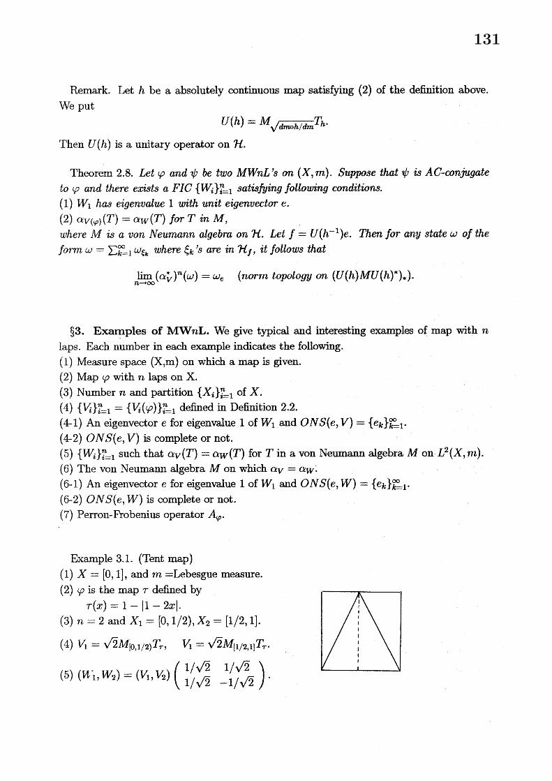
Example 3.1. (Tent map)(1) $X=[0,1]$ , and $m=\mathrm{L}\mathrm{e}\mathrm{b}\mathrm{e}\mathrm{s}\mathrm{g}\mathrm{u}\mathrm{e}$ measure.(2) $\varphi$ is the map $\tau$ defined by

$\tau(x)=1-|1-2X|$ .$||l|$

(3) $n=2$ and $X_{1}=[0,1/2),$ $X_{2}=[1/2,1]$ . $\mathrm{t}$

$\}$

(4) $V_{1}=\sqrt{2}M_{[0,1/)}2\tau_{\mathcal{T}}$ , $V_{1}=\sqrt{2}M_{[1/2,11}T_{\tau}$ . $\iota$

$\}$

\dagger

(5) $(w_{1}^{\vee}, W_{2})=(V_{1}, V2)(1/\sqrt{2}1/\sqrt{2}-1/\sqrt{2}1/\sqrt{2})$ .1

131

(6) $M=B(L^{2}[0,1])$

(6-1) $e(x)=1(x\in[0,1])$ and $e_{1}=e,$ $e_{2}=M_{1^{0,1/2}}$) $e_{1^{-}}M\iota 1/2,1$ ] $e1$ .(6-2) $ONs(e, W)$ is complete.

(7) $A_{\tau}( \eta)(X)=\frac{1}{2}(\eta(\frac{x}{2})+\eta(1-\frac{x}{2}))$ .

$\overline{!\mathrm{t}||\mathrm{I}\iota,}$

$.\Gamma_{1}||$. $\overline{||\mathrm{t}.}$

$\bigwedge_{1,!!}\underline{||\mathrm{J}|}$

$.. \frac{l!|1||}{||\mathrm{I}\mathrm{I}\mathrm{t}|:||}.\cdot\dot{.}.$.$\mathrm{e}_{1}$

.$\mathrm{e}_{\alpha}$

$\mathrm{e}_{3}$$\mathrm{e}_{4}$

Example 3.2. (Generalized tent map)(1) $X=[0,1]$ , and $m=\mathrm{L}\mathrm{e}\mathrm{b}\mathrm{e}\mathrm{s}\mathrm{g}\mathrm{u}\mathrm{e}$ measure.(2) $\varphi=\tau_{c},$ $(0$

$\varphi_{c}(_{X})=\{$

(3) $n=2$ and

(4) $V_{1}=M_{\sqrt{1/}}$

$<c<1)$ defined by$\frac{1}{\Gamma,}x$ for $0\leq x\leq c$,$\frac{1}{c-1}(x-1)$ for $c<x\leq 1$ .

$X_{1}=[0,1/2),X_{2}=[1/2,1]$ .

$cM,T\chi_{[0_{\mathrm{c}}]}\tau_{\mathrm{c}}$

’ $V_{2}=M_{\sqrt{1/(1-c\rangle}1}M\tau\chi_{\mathrm{l}_{C},1}\tau_{c}$ .

$.\ovalbox{\tt\small REJECT}_{\iota}^{\iota}\mathrm{t}1\iota_{1}\mathrm{I}1$

(5) $(W_{1}, W_{2})=(V_{1}, V2)(\sqrt{c}\sqrt{1-c}\sqrt{1-c}-\sqrt{c})$ .

(6) $M=B(L^{2}[0,1])$

(6-1) $e(x)=1(x\in[0,1])$ and $e_{1}=e,$ $e_{2}(x)=\{$$\frac{1}{\sqrt{c}}$ for $0\leq x\leq c$,$-\sqrt{c-1}1$ for $c<x\leq 1$ .

(6-2) $ONS(e, W)$ is complete.(7) $A_{\tau_{c}}(\eta)(X)=C(\eta(_{C}X))+(1-c)\eta((_{\mathrm{C}}-1)_{X+}1))$.

$\ulcorner||\overline{|t}$

$\downarrow$.$\iota$

$\mathrm{t}$

$|,$

$*|.\overline{\underline{1\iota l.}}$

$\mathrm{e}_{\iota}$

$\mathrm{e}_{2}$

Remark. $\tau_{c}$ and $\tau_{\mathrm{c}}$ are topologically conjugate $(\mathrm{c}\mathrm{f}.[6],[8])$ but they are $\mathrm{A}\mathrm{C}$-conjugate onlyif $c=d$.

Example 3.3.($\mathrm{L}\mathrm{o}\mathrm{g}\mathrm{i}_{\mathrm{S}\mathrm{t}}\mathrm{i}\mathrm{C}$ map) $(\mathrm{c}\mathrm{f}.[9])$

(1) $X=[0,1]$ , and $m=\mathrm{L}\mathrm{e}\mathrm{b}\mathrm{e}\mathrm{s}\mathrm{g}\mathrm{u}\mathrm{e}$ measure.(2) $\varphi$ is the map $\lambda$ defined by

$\lambda(x)=4x(1-x)(3)n=2$ and $X_{1}=[0,1/2),X_{2}=[1/2,1]$ .

132

$\mathrm{c}_{1}$ $\mathrm{c}_{2}$ $\mathrm{c}_{-3}$ c4(The logistic map is topologically conjugate to the tent map with conjugacy

$h(x)=\sin^{2}(\pi x/2)(\mathrm{c}\mathrm{f}.[7]))$ .

Example 3.4. (Typical map with 3 laps)(1) $X=[0,1]$ , and $m=\mathrm{L}\mathrm{e}\mathrm{b}\mathrm{e}\mathrm{s}\mathrm{g}\mathrm{u}\mathrm{e}$ measure.(2) $\varphi$ is the map defined by

$\varphi(x)=\{$

$3x$ for $0\leq x<1/3$ ,$3x-1$ for $1/3\leq x<2/3$ ,$3x-2$ for $2/3\leq x\leq 1$ .

(3) $n=3$ and $X_{1}=[0,1/3),X_{2}=[1/3,2/3),X_{2}=[2/3,1]$ .

(4) $V_{1}=\sqrt{3}M_{\chi}T_{\varphi}10,1/3)$’

$V_{2}=\sqrt{3}M_{x_{1^{1/3,2}}/)}T_{\varphi}3$’

$V_{3}=\sqrt{3}M_{x_{\mathrm{I}2/1}\varphi}\tau 3,1^{\cdot}$

(5) $(W_{1}, W_{2}, W_{3})=(V1, V2, V3)(1/\sqrt{3}1/\sqrt{3}1/\sqrt{3}(-3^{-}-\sqrt{3})/6(31/\sqrt{3}\sqrt{3})/6$ $(-3-\sqrt{3})/(3-\sqrt{3})1/\sqrt{3}/66)$ .

(6) $M=B(L^{2}[\mathrm{o}, 1])$

(6-1) $e(x)=1(x\in[0,1])$ and $e_{1}=e,$$e_{2}(x)= \chi_{[0,1/3)}+\frac{\sqrt{3}-1}{2}\chi_{[1/3},2/3)+\frac{-\sqrt{3}-1}{2}\chi[2/3,1]$ ,

$e_{3}(X)=x1^{0},1/3)+ \frac{-\sqrt{3}-1}{2}x_{[1}/3,2/3)+\frac{\sqrt{3}-1}{2}\chi 12/3,11$ .(6-2) $ONS(e, W)$ is complete.

(7) $A_{\varphi}( \eta)(X)=\frac{1}{3}(\eta(\frac{x}{3})+\eta(\frac{x}{3}+\frac{1}{3})+\eta(\frac{x}{3}+\frac{2}{3}))$ .

$\overline{.}\bigwedge_{\mathrm{I}}^{\mathrm{t}}||||-|\iota|$

$\mathrm{e}_{\mathrm{I}}$

$\mathrm{e}_{3}$ $\underline{\mathrm{t}1}!$

’

133

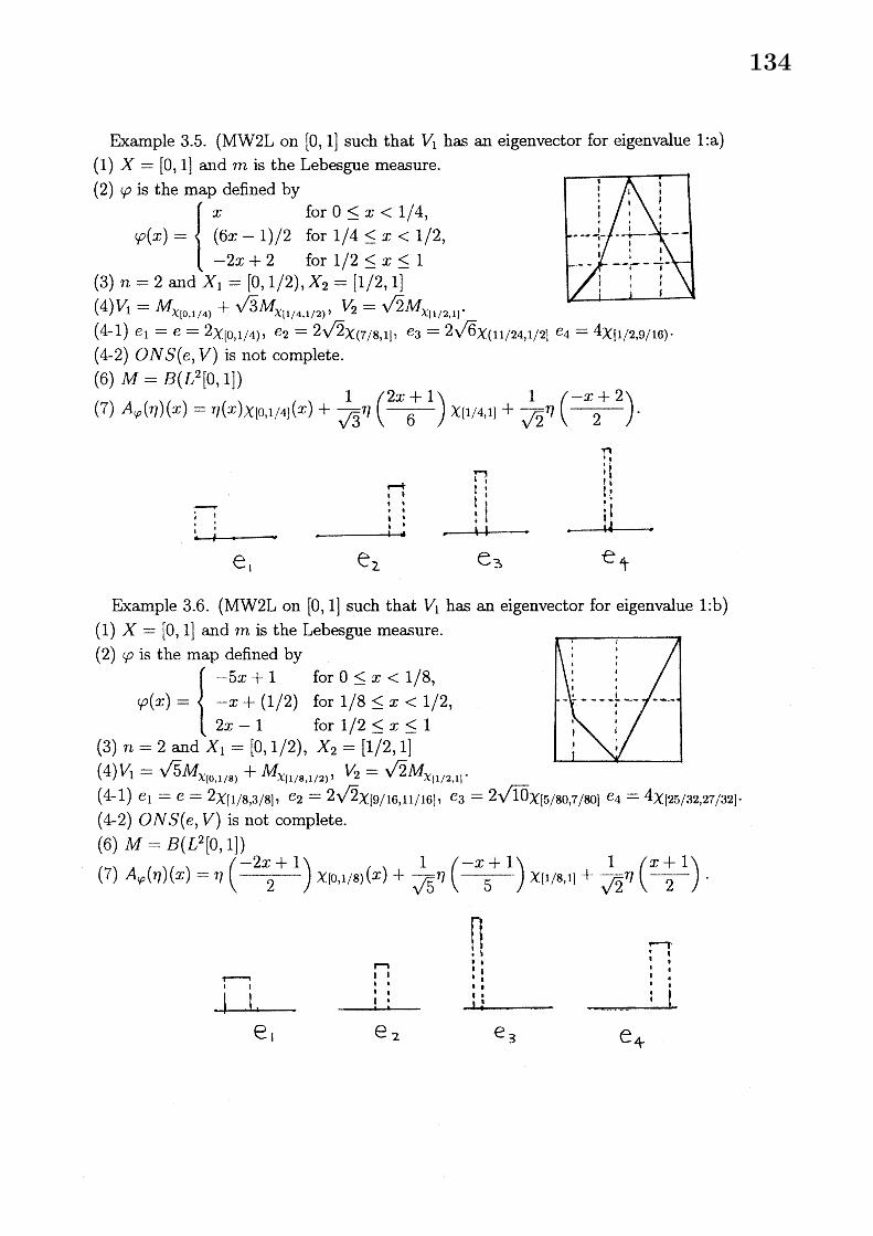
Example 3.5. ( $\mathrm{M}\mathrm{W}2\mathrm{L}$ on $[0,1]$ such that $V_{1}$ has an eigenvector for eigenvalue $1:\mathrm{a}$)(1) $X=[0,1]$(2) $\varphi$ is the $\mathrm{m}$

$\varphi(x)=\{$

(3) $n=2$ and(4) $V_{1}=M_{\lambda_{1}0,1}$

and $m$ is the Lebesgue measure.ap defined by

$x$ for $0\leq x<1/4$ ,$(6x-1)/2$ for $1/4\leq x<1/2$ ,$-2x+2$ for $1/2\leq x\leq 1$

$X_{1}=[0,1/2),$ $X_{2}=[1/2,1]$

$+\sqrt{3}M_{\lambda}\mathrm{l}1/4,1/2)’ V_{2}=\sqrt{2}M_{x_{1}}1/2,1\mathrm{l}$ ./4)

$.’. \ovalbox{\tt\small REJECT}\sim\wedge\sim_{\dagger^{-\frac{1\mathrm{i}}{1}-}}^{\mathrm{I}}..’,arrow--|:|\prime \mathrm{t}11\mathrm{t}|’\dagger-arrow\ulcorner||(\wedge\frac{1}{1}-||\mathrm{I}\}t$

(4-1) $e_{1}=e=2\chi_{[0,1/4)},$ $e_{2}=2\sqrt{2}\chi(\tau/8,11, e_{3}=2\sqrt{6}x_{(11/2}4,1/2]e_{4}=4x[1/2,9/16)$ .(4-2) $ONS(e, V)$ is not complete.(6) $M=B(L^{2}[0,1])$

(7) $A_{\varphi}( \eta)(X)=\eta(x)x\iota 0,1/4](X)+\frac{1}{\sqrt{3}}\eta(\frac{2x+1}{6})x_{11}/4,1]+\frac{1}{\sqrt{2}}\eta(\frac{-x+2}{2})$ .

$\overline{!|1\mathrm{t}.}$

$\underline{\overline{:\iota.|\dagger,}}$ $\underline{!.i.}$

$\mathrm{e}_{1}$$\mathrm{e}_{\mathrm{Z}}$

$\mathrm{e}_{3}$ $\mathrm{e}_{+}$

Example 3.6. ( $\mathrm{M}\mathrm{W}2\mathrm{L}$ on $[0,1]$ such that $V_{1}$ has an eigenvector for eigenvalue $1:\mathrm{b}$ )(1) $X=[0,1]$(2) $\varphi$ is the $\mathrm{m}$

$\varphi(x)=\{$

(3) $n=2$ and(4) $V_{1}=\sqrt{5}M$

and $m$ is the Lebesgue measure.ap defined by

$-5x+1$ for $0\leq x<1/8$ ,$-X+(1/2)$ for $1/8\leq x<1/2$ ,$2x-1$ for $1/2\leq x\leq 1$

$X_{1}=[0,1/2),$ $X_{2}=[1/2,1]$

$x_{|0},1/8)+Mx_{\mathrm{l}1}/8,1/2)’ V_{2}=\sqrt{2}M_{x_{1/}1\mathrm{l}}12,\cdot$

$\ovalbox{\tt\small REJECT}_{l^{-\sim}}^{\vee\sim}-- 1|\dagger^{---}|\mathrm{t}t|||i.’\sim-$

(4-1) $e_{1}=e=2\chi[1/8,3/8],$ $e_{2}=2\sqrt{2}x_{19/1/}16,1161,$ $e_{3}=2\sqrt{10}x_{[5/8}\mathrm{o},7/80]e_{4}=4x_{125}/32,27/32]$.(4-2) $ONS(e, V)$ is not complete.(6) $M=B(L^{2}[\mathrm{o}, 1])$

(7) $A_{\varphi}( \eta)(x)=\eta(\frac{-2x+1}{2})x_{1^{0},1}/8)(x)+\frac{1}{\sqrt{5}}\eta(\frac{-x+1}{5})\chi_{[}1/8,11^{+}\frac{1}{\sqrt{2}}\eta(\frac{x+1}{2})$ .

$..\lceil|||\downarrow|i$

. $\neg \mathrm{l}\dot{\mathrm{t}}\mathrm{t}|$.$|||\iota|\iota 1r\neg$. ”

$|\mathrm{I}$ : $\underline{||.:|}$

$\mathrm{e}_{\mathrm{I}}$ $\mathrm{e}_{2}$$\mathrm{e}_{3}$

$\mathrm{e}_{+}$

134

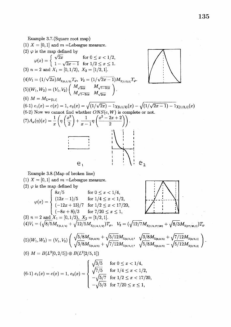
Example $3.7.$ ( $\mathrm{s}_{\mathrm{q}\mathrm{u}}\mathrm{a}\mathrm{r}\mathrm{e}$ root map)(1) $X=[0, \mathrm{I}]$ and $m=\mathrm{L}\mathrm{e}\mathrm{b}\mathrm{e}\mathrm{s}\mathrm{g}\mathrm{u}\mathrm{e}$ measure.(2) $\varphi$ is the $\mathrm{m}$

$\varphi(x)=\{$

(3) $n=2$ and

(4) $V_{1}=(1/\sqrt{2}$

ap defined by$\sqrt{2x}$ for $0\leq x<1/2$ ,$1-\sqrt{2x-1}$ for $1/2\leq x\leq 1$ .

$X_{1}=[0,1/2),$ $X_{2}=[1/2,1]$ .

$x)M_{x_{1^{0}},2}\tau_{\varphi}1/)’ V_{2}=(1/\sqrt{2x-1})M_{\chi_{\mathrm{l}1/1}}\tau_{\varphi}2,1^{\cdot}$

$\ovalbox{\tt\small REJECT}_{\iota}^{1}\iota_{\dagger}||\mathrm{t}11$

(5) $(W_{1}, W2)=(V1, V2)$ .(6) $M=M_{L}\infty[0,1]$

(6-1) $e_{1}(x)=e(x)=1,$ $e_{2}(x)=\sqrt{(1/\sqrt{2x})-1}\chi_{10},1/2)(X)-\sqrt{(1/\sqrt{2x-1})-1}x_{[/}12,11(x)$

(6-2) Now we cannot find whether $ONS(e, W)$ is complete or not.

(7) $A_{\varphi}( \eta)(X)=\frac{1}{x}(\eta(\frac{x^{2}}{2})+\frac{1}{x-1}\eta(\frac{x^{2}-2X+2}{2}))$ .

$\downarrow$

$\underline{||t.}$

$\mathrm{e}_{\iota}$$\mathrm{e}_{\mathrm{z}}$

(5) $(W_{1,2}W)=(V1, V2)(\sqrt{5/8}M_{\chi_{1}0},+\sqrt{5/12}2/5)M\sqrt{3/8}M_{\chi_{12/5})}+\sqrt{7/12}0’ Mx_{|2/1}\chi \mathrm{l}2/5,115,1’$

,$\sqrt{3/8}M_{x_{|\mathrm{O},2}/},+\sqrt{7/12}5)M\sqrt{5/8}M_{\chi_{1^{\mathrm{o}}2})}-/5\sqrt{5/12}Mx_{\mathrm{l}2}/\mathrm{s},1\mathrm{l}\chi_{12}/5,11)$

(6) $M=B(L^{2}[\mathrm{o}, 2/5])\oplus B(L^{2}[2/5,1])$

(6-1) $e_{1}(x)=e(x)=1,$ $e_{2}(x)=\{$

$\sqrt{3/5}$ for $0\leq x<1/4$ ,$\sqrt{7/5}$ for $1/4\leq x<1/2$ ,$-\sqrt{5/7}$ for $1/2\leq x<17/20$ ,$-\sqrt{5/3}$ for $7/20\leq x\leq 1$ ,

135

(6-2) Now we cannot find whether $ONS(e, W)$ is complete or not.

(7) $A_{\varphi}( \eta)(X)=\frac{5}{8}\eta(\frac{5x}{8})x_{10},2/5\rangle(x)+\frac{5}{12}\eta(\frac{5x+1}{12})\chi_{1^{2}}/5,11(x)$

$+ \frac{3}{8}\eta(\frac{-3x+8}{8})x_{10,2}/5)(x)+\frac{7}{12}\eta(\frac{-7x+13}{12})x_{[2/5,1}1(x)$.

$(\tau 3l^{n4}=\mathrm{a}\mathrm{n}\mathrm{Q}\mathrm{A}_{1\mathrm{L}}=\cup, \perp/\angle^{-})\cross\lfloor^{\cup},$ $\perp/\angle),$ $\mathrm{A}_{2}=_{\mathrm{L}^{\perp}}/\angle,$ $\perp\rfloor\cross\lfloor\cup,$ $1/\angle l$ , A3 $=_{\mathrm{L}^{\perp}}/\angle,$ $1\rfloor\cross_{\mathrm{t}^{\perp}}/\vee\angle,$ $1\rfloor,$ $\mathrm{x}_{4}=$

$[0,1/2)\cross[1/2,1]$ .

(4) $V_{1}=2M_{\chi_{1^{0},1}\mathrm{x})}T/2)10,1/2\varphi’ V_{2}=2M_{x_{\mathrm{I}1/2},\mathrm{x}/}T1\mathrm{l}\mathrm{I}\mathrm{O},12)\varphi’ V_{3}=2M_{x_{\mathrm{I}^{\mathrm{o}},1}2}\tau_{\varphi}/|\mathrm{X}\iota 1/2,1|’ V_{4}=2M_{\chi_{\mathrm{I}}/2,1|}T_{\varphi}1/2,11\cross 11^{\cdot}$

(5) $(W_{1}, W_{2}, W_{3}, W_{4})=(V_{1}, V_{2}, V_{3}, V_{4})$

(6) $M=B(L^{2}([\mathrm{o}, 1]\cross[0,1]))$

(6-1) $e_{1}(x,y)=e(x, y)=1((x, y)\in[0,1]\cross[0,1])$ and$e_{2}(x)=x_{[1}\mathrm{o},/2)\cross\iota 0,1/2)-x_{[1}/2,1]\mathrm{X}\iota 0,1/2)+\chi_{1^{0,1}/}2]\cross[1/2,11-x[1/2,1]\cross[1/2,1]$ .(6-2) $ONS(e, W)$ is complete.

(7) $A_{\varphi}( \eta)(X)=\frac{1}{4}(\eta+\eta(1-\frac{x}{2},$ $\frac{x}{2})+\eta(\frac{x}{2},1-\frac{x}{2})+\eta(1-\frac{T}{2},1-\frac{x}{2}))$ .

$\mathrm{e}_{1}$$\mathrm{e}_{\mathit{2}}$

Example 3.10. (Baker’s transformation)(1) $X=[0,1]\cross[0,1]$ and $m=\mathrm{L}\mathrm{e}\mathrm{b}\mathrm{e}\mathrm{s}\mathrm{g}\mathrm{u}\mathrm{e}$ measure.(2) $\varphi$ is the map $\beta$ defined by

136

$\beta(x, y)=\{$$(2x,y/2)$ for $0\leq x<1/2$ ,$(2x-1, (y+1)/2)$ for $1/2\leq x\leq 1$ .

(3) $n=1$ a.n$\mathrm{d}x1=X$

(4) $V_{1}=T_{\beta}$

(4-1) $e_{1}(x,y)=e(x, y)=1$

(4-2) $ONS(e, W)=\{e_{1}\}$ is not complete.(6) $M=B(L^{2}([0,1]\cross[0,1]))$

(7) $A_{\beta}(\eta)(x)=\eta(\beta(x))$

$\mathrm{e}_{t}$

Remark. Baker’s transformation is strong-mixing but $\{(\alpha_{V}^{*})^{n}(\omega_{\zeta})\}_{n=1}^{\infty}$ does not convergesto $\omega_{e}$ in the norm topology in $M_{*}$ .

Example $3.11.$ ( $\mathrm{U}\dot{\mathrm{m}}\mathrm{l}\mathrm{a}\mathrm{t}\mathrm{e}\mathrm{r}\mathrm{a}\mathrm{l}$ shift map)(1) $X= \prod_{n=1}^{\infty}\{1,2\}$ and $m=\mathrm{u}\mathrm{s}\mathrm{u}\mathrm{a}\mathrm{l}$ measure.(2) $\varphi$ is the map $\sigma$ defined by

$\sigma((_{X_{\mathrm{l}}x\tau_{\text{ノ}}},2,3, \ldots))=(X_{2,3,4}X_{J}X, \ldots)$ ,(3) $n=2$ and $X_{1}=X(1)=\{(x_{n})_{n=1}^{\infty}\in X|x_{1}=1\},$ $x_{2}=X(2)=\{(x_{n})_{n=}^{\infty}1\in X|x1=2\}$

(4) $V_{1}=\sqrt{2}MX(1)\tau_{\sigma}$ , $V_{1}=\sqrt{2}MX(2)\tau_{\sigma}$ .

(5) $(W_{1}, W_{2})=(V_{1}, V2)(1/\sqrt{2}1/\sqrt{2}-1/\sqrt{2}1/\sqrt{2})$ .(6) $M=B(L2(x))$(6-1) $e(X)=1(x\in X)$ and $e_{1}=e,$ $e_{2}=x\mathrm{x}(1)e_{1}-\chi X(2)e1$ .(6-2) $ONS(e, W)$ is complete.(7) $A_{\sigma}( \eta)(_{X})=\frac{1}{2}(\eta(\gamma_{1})+\eta(\gamma 2))$ ,where $\gamma_{1}((x_{1},x_{2},x_{3}, \ldots))=(1,x_{1},x_{2}, \ldots)$ and $\gamma 2((X1,X2)X3,$ $\ldots))=(2, x_{1}, X_{2}, \ldots)$ .

137

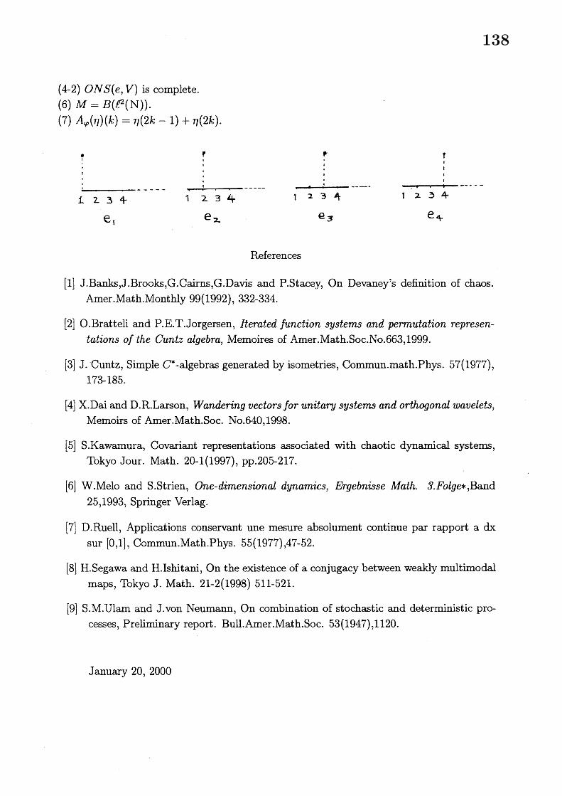
(4-2) $ONS(e, V)$ is complete.(6) $M=B(\ell 2(\mathrm{N}))$ .(7) $A_{\varphi}(\eta)(k)=\eta(2k-1)+\eta(2k)$ .

$|$

. ’ $p$$\gamma$

$\mathrm{t}$

$t$

$\iota$ 1$\mathrm{r}$ .

$\mathfrak{l}$

’’ 1$arrow—–$ $\underline{11}-----$ $.\underline{\iota}-----$

$f$. $\mathrm{Z}3+$ 1 2. 3 $*$ 1 2 3 4 $\uparrow$ $\mathrm{z}$ $3+$

$\mathrm{e}_{\mathrm{f}}$

$\mathrm{e}_{2}$. $\mathrm{e}_{3}$ $\mathrm{e}_{+}$

References

[1] J.Banks,J.Brooks,G.Cairns,G.Davis and P.Stacey, On Devaney’s definition of chaos.Amer.Math.Monthly 99(1992), 332-334.

[2] O.Bratteli and P.E.T.Jorgersen, Iterated function systems and permutation represen-tations of the Cuntz algebra, Memoires of Amer.Math.Soc.No.663,1999.

[3] J. Cuntz, Simple $C^{*}$-algebras generated by isometries, Commun.math.Phys. 57(1977),173-185.

[4] X.Dai and D.R.Larson, Wandering vectors for unitary system8 and orthogonal wavelet8,Memoirs of Amer.Math.Soc. No.640,1998.

[5] S.Kawamura, Covariant representations associated with chaotic dynamical systems,Tokyo Jour. Math. 20-1 (1997), pp.205-217.

[6] W.Melo and S.Strien, One-dimensiond $dynamiCs_{y}$ Ergebnisse Math. $\mathit{3}.Fo\iota_{ge*},\mathrm{B}\mathrm{a}\mathrm{n}\mathrm{d}$

25,1993, Springer Verlag.

[7] D.Ruell, Applications conservant une mesure absolument continue par rapport a dxsur [0,1], Commun.Math.Phys. 55(1977),47-52.

[8] H.Segawa and H.Ishitani, On the existence of a conjugacy between weakly multimodalmaps, Tokyo J. Math. 21-2(1998) 511-521.

[9] S.M.Ulam and J.von Neumann, On combination of stochastic and deterministic pro-cesses, Preliminary report. Bull.Amer.Math.Soc. 53(1947),1120.

January 20, 2000

138