development of parametric robust control design … 数式処理第13 巻第2 号2007 control...

数式処理 J.JSSAC (2007)Vol. 13, No. 2, pp. 3 - 25

奨励賞論文

Development ofParametric Robust Control Design Toolbox

Noriko Hyodo ∗

AlphaOmega Inc.

(Received 2007/1/15)

Abstract

A lot of important control system design problems are regarded as parametric and non-convex opti-mization problems. Parametric robust control design toolbox solves these robust control problems andvisualize the feasible parameter regions via a parameter space approach based on symbolic-numericcomputation. This paper shows a method of solving robust control system design problems by usingsymbolic-numeric computation and description of parametric robust control design toolbox.

1 IntroductionControl system design is to find out feasible parameters to be designed for which a target systemsatisfies given control design specifications. A lot of important control system design problemsare regarded as parametric and non-convex optimization problems, and of course to solve theseproblems only by using numeric computation is difficult. Recently, there has been an increasinginterest in the application of computer algebra to control system analysis and design.

We have been developing the parametric robust control design toolbox. This toolbox solves therobust control design problems by parameter space approach based on symbolic-numeric compu-tation, and visualize the feasible parameter regions of robust control design problems. By usingsymbolic computation, this toolbox solves the robust control problems exactly. This toolbox usesquantifier elimination(QE) by symbolic computation.

2 Robust controller design by a parameter space approachA parameter space approach is known to control community as an effective method for robustcontrol synthesis and multi-objective design of fixed-structure controllers. Multi-objective robustcontrol problem is one of main concerns in control theory. But it often the case that these robust

∗[email protected]

c© 2007 Japan Society for Symbolic and Algebraic Computation

4 数式処理第 13巻第 2号 2007

control problems are regarded as nonlinear and non-convex optimization problems. We have pro-posed a method with a software tool for parametric robust control synthesis by symbolic-numericcomputation which can solve above problems. The method is based on a parameter space approachaccomplished by using QE. This section shows the algorithm, methods and solving procedures ofparameter space approach that are used in parametric robust control design toolbox.

2.1 Design procedure

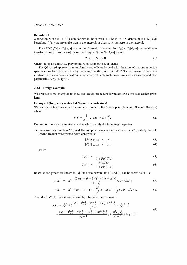
K(s) P (s)r e u y

− +

Fig. 1: A feedback control system

Now let us consider a feedback control system as shown in Fig.1, and propose a scheme forfixed-structure robust controller synthesis based on a parameter space approach as follows:

1. According to the characteristics of the plant and also design requirements, determine the struc-ture of a class of controllers K and select the design parameters in K . For instance, when thePI-controller K(s) = k + m

s is chosen, k and m are the parameters to be designed.

2. Reduce the given specifications φi to the equivalent first-order formulas ψi.

3. Compute the admissible regions of the design parameters for all specifications φi by applyingQE to the first-order formulas ψi derived from φi.

4. Superpose the admissible regions in the parameter space. Then we can take appropriate param-eters from the intersections by considering other specifications.

In Step 2, most of important design specifications for robust control such as frequency re-stricted H∞ norm constraints, stability (gain/phase) margin and stability radius specifications, andpole location requirements can be recast as sign definite condition (1) by using simple symboliccomputations [6],[8]. This is beneficial to achieve Step 3 efficiently.

In Step 3, a specialized QE algorithm using Sturm-Habicht sequence [2], which is more efficientthan a general QE algorithm based on cylindrical algebraic decomposition, can be applied forsolving a sign definite condition [1]. By using specialized QE, nonlinear and non-convex problemscould be solved exactly. QE-based method provides us an exact and whole feasible regions of thedesign parameters.

2.2 Sign definite conditionIn this toolbox, selected specifications are reduced to the equivalent first-order formulas that iscalled sign definite condition(SDC). This is a definition of sign definite condition(see [6] for de-tails).

J.JSSAC Vol. 13, No. 2, 2007 5

Definition 1A function f (x) : R 7→ R is sign definite in the interval x ∈ [a, b], a < b, denote f (x) ∈ N0[a, b]hereafter, if f (x) preserves the sign in the interval, or does not cross zero in the interval.

Then SDC f (x) ∈ N0[a, b] can be transformed to the condition f (z) ∈ N0[0,∞] by the bilineartransformation z = −(x − a)/(x − b). Put simply, f (z) ∈ N0[0,∞] means

∀z > 0, f (z) > 0 (1)

where f (z) is an univariate polynomial with parametric coefficients.The QE-based approach can uniformly and efficiently deal with the most of important design

specifications for robust control by reducing specifications into SDC. Though some of the spec-ifications are non-convex constraints, we can deal with such non-convex cases exactly and alsoparametrically by using QE.

2.2.1 Design examples

We propose some examples to show our design procedure for parametric controller design prob-lems.

Example 2 (frequency restricted H∞-norm constraints)We consider a feedback control system as shown in Fig.1 with plant P(s) and PI-controller C(s)where

P(s) =1

s − 1, C(s) = k +

ms. (2)

Our aim is to obtain parameters k and m which satisfy the following properties:

• the sensitivity function S (s) and the complementary sensitivity function T (s) satisfy the fol-lowing frequency restricted norm constraints:

‖S (s)‖[0,ωs] < γs, (3)‖T (s)‖[ωt ,∞] < γt, (4)

where

S (s) =1

1 + P(s)C(s), (5)

T (s) =P(s)C(s)

1 + P(s)C(s). (6)

Based on the procedure shown in [6], the norm constraints (3) and (4) can be recast as SDCs.

fs(x) = x2 +(2mγ2

s − (k − 1)2γ2s + 1)x + m2γ2

s

−1 + γ2s

∈ N0[0, ω2s], (7)

ft(x) = x2 + (2m − (k − 1)2 +k2

γ2t

)x + m2(1 − 1γ2

t) ∈ N0[ω2

t ,∞]. (8)

Then the SDC (7) and (8) are reduced by a bilinear transformation

fs(z) = γ4sz3 + (

((k − 1)2γ2s − 2mγ2

s − 1)ω4s + m2γ2

s

γ2s − 1

− γ4sω

2s)z2

− ((k − 1)2γ2s − 2mγ2

s − 1)ω2s + 2m2ω2

sγ2s

γ2s − 1

z +m2ω4

sγ2s

γ2s − 1

∈ N0[0,∞],(9)


ft(z) = z2 + (2m − (k − 1)2 +k2

γ2t− 2ωt)z + ω4

t − ω2t (2m − (k − 1)2 +

k2

γ2t

)

+ m2(1 − 1γ2

t) ∈ N0[0,∞].

(10)

By using QE to solve SDC (9) and (10), we obtain feasible regions. Then we can get the feasibleregions of controller parameters so that the system (2) satisfies the mixed sensitivity specification.

Example 3 (Gain margin constraint)Gain margin constraint can be reduced to a sign definite condition as follows (see [8]). Consider atransfer function G(s) and decompose G( jω) as

G( jω) =gr(ω) + jg j(ω)

d(ω)(11)

where gr(ω), g j(ω) and d(ω) are polynomials in ω.As shown in [8], G(s) holds the gain margin (γm, γ

M) iff the following system of equations f1(ω, t) = gr(ω) − d(ω)t = 0f2(ω) = g j(ω) = 0

is not satisfied in ω ∈ R, t ∈ [−1/γm,−1/γM]. One can obtain a polynomial fg(t) by eliminating ωfrom f1, f2. Then the condition that G(s) holds the gain margin (γm, γ

M) can be reduced to a signdefinite condition, that is, fg(t) is sign definite in t ∈ [−1/γm,−1/γM]. By bilinear transformation,we can get the fg(z) ∈ [0,∞].

Example 4 (Phase margin constraint)Phase margin constraint can be reduced to a sign definite condition as follows (see [8]). As thein the case of gain margin constraint, consider a transfer function G(s) and decompose G( jω) (see(11)).

As shown in [8], G(s) holds the phase margin φ iff the following system of equations f1(ω) = g2r (ω) + g2

j (ω) − d2(ω) = 0

f2(ω, t) = gr(ω) − d(ω)t = 0

is not satisfied in ω ∈ R, t ∈ [−1, cos(−π+ φ)]. One can obtain a polynomial fp(t) by eliminating ωfrom f1, f2. Then the condition that G(s) holds the phase margin φ can be reduced to a sign definitecondition, that is, fp(t) is sign definite in t ∈ [−1, cos(−π + φ)]. By bilinear transformation, we canget the fp(z) ∈ [0,∞].

Example 5 (Pole location(Wedge shape))For the wedge shape region, x + jy ∈ D can be expressed as x = ω

y = m(ω − t), ω ∈ R, t ∈ [b,∞].

Let us consider how to assign all roots of a characteristic polynomial p(s) in the specified regionD ∈ C. This is equivalent to

p(s) , 0, ∀s ∈ D

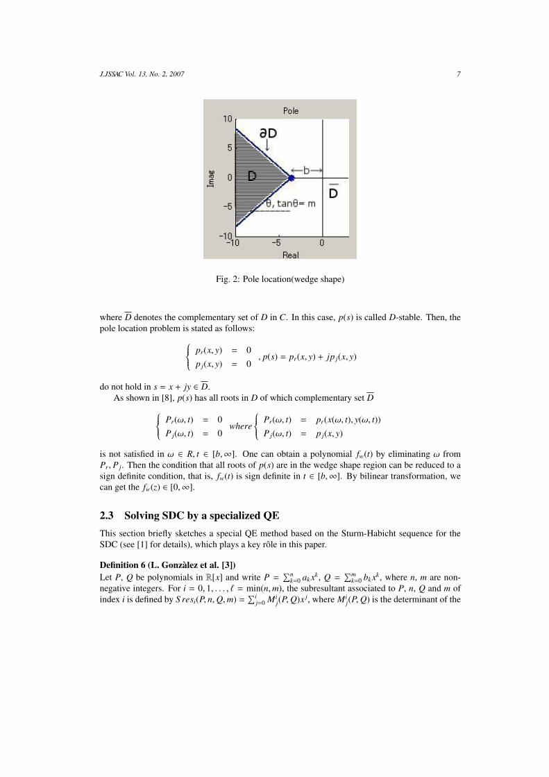
J.JSSAC Vol. 13, No. 2, 2007 7

Fig. 2: Pole location(wedge shape)

where D denotes the complementary set of D in C. In this case, p(s) is called D-stable. Then, thepole location problem is stated as follows: pr(x, y) = 0

p j(x, y) = 0, p(s) = pr(x, y) + jp j(x, y)

do not hold in s = x + jy ∈ D.As shown in [8], p(s) has all roots in D of which complementary set D Pr(ω, t) = 0

P j(ω, t) = 0where

Pr(ω, t) = pr(x(ω, t), y(ω, t))P j(ω, t) = p j(x, y)

is not satisfied in ω ∈ R, t ∈ [b,∞]. One can obtain a polynomial fw(t) by eliminating ω fromPr, P j. Then the condition that all roots of p(s) are in the wedge shape region can be reduced to asign definite condition, that is, fw(t) is sign definite in t ∈ [b,∞]. By bilinear transformation, wecan get the fw(z) ∈ [0,∞].

2.3 Solving SDC by a specialized QEThis section briefly sketches a special QE method based on the Sturm-Habicht sequence for theSDC (see [1] for details), which plays a key rôle in this paper.

Definition 6 (L. Gonzàlez et al. [3])Let P, Q be polynomials in R[x] and write P =

∑nk=0 ak xk, Q =

∑mk=0 bk xk, where n, m are non-

negative integers. For i = 0, 1, . . . , ` = min(n,m), the subresultant associated to P, n, Q and m ofindex i is defined by S resi(P, n,Q,m) =

∑ij=0 Mi

j(P,Q)x j, where Mij(P,Q) is the determinant of the


matrix composed by the columns 1, 2, . . . , n + m − 2i − 1 and n + m − i − j in the matrix

si(P, n,Q,m) :=

n+m−i︷︸︸︷

an . . . a0

. . .. . .

an . . . a0

bm . . . b0

. . .. . .

bm . . . b0

m − i

n − i

Let v = n + m − 1 and δk = (−1)k(k+1)

2 . The Sturm-Habicht sequence associated to P and Q is thendefined as the list of polynomials {S H j(P,Q)} j=0,...,v+1 given by

S Hv+1(P,Q) = P ,

S Hv(P,Q) = P′Q ,

S H j(P,Q) = δv− j · S res j(P, p, P′Q, v)for j = 0, 1, . . . , v − 1 ,

where P′ = dPdx . In particular, {S H j(P, 1)} j=0,...,v+1 is called the Sturm-Habicht sequence of P. Here

it is simply denoted by {S H j(P)}.

The Sturm-Habicht sequence can be used for real root counting, just like the Sturm sequence.Moreover it has favourable properties in terms of specialization and computational complexity (see[3, 4] for details).

Theorem 7 (González-Vega et al. [4])Let P(x) ∈ R[x] and

{g0(x), . . . , gk(x)}be a set of polynomials obtained from {S H j(P(x))} by deleting the identically zero polynomials.Let α, β ∈ R ∪ {−∞,+∞} and α < β. Define WS H(P;α) as the number of sign variations on{g0(α), . . . , gk(α)}. Then, WS H(P;α, β) := WS H(P;α)−WS H(P; β) gives the number of real roots ofP in [α, β].

Denote the principal j-th Sturm-Habicht coefficient of S H j( f ), i.e., the coefficient of degree jof S H j( f ), by st j( f ) and a constant term of S H j( f ) by ct j( f ) for all j. Then,

WS H( f ; 0,+∞) = WS H( f ; 0) −WS H( f ;+∞)= V

({ctn( f ), . . . , ct0( f )}

)− V({stn( f ), . . . , st0( f )}

), (12)

where V({ai})

stands for the number of sign changes over the sequence {ai}.The SDC holds if and only if both WS H ( f ; 0, +∞) = 0 and stn( f ) > 0 hold.Hence an equivalent condition to the SDC can be obtained through the following combinatorial

procedure:

1. Consider all (at most) 32n−1 possible sign combinations over the polynomials cti( f ),sti( f ) since ct0( f ) = st0( f ), stn( f ) > 0, stn−1( f ) > 0.

J.JSSAC Vol. 13, No. 2, 2007 9

2. Choose all sign conditions that satisfy WS H( f ; 0, +∞) = 0 by (12).

3. Construct semi-algebraic sets generated by cti( f ), sti( f ) for the selected sign conditions andcombine them as a union.

The obtained condition is of the form of a union of semi-algebraic sets, so called disjunctivenormal form. (The obtained result is expected to contain many empty sets. Some impossible signcombinations can be pruned beforehand (see [1]).)

3 Parametric robust control design toolboxOur parametric robust control design toolbox is a GUI-based parametric robust control toolbox.And this toolbox is also based on symbolic quantifier elimination cooperating with numerical sim-ulation.

To use Maple/MATLAB as a platform has the advantage that Maple packages are automaticallyincorporated into MATLAB by using “MATLAB Extended Symbolic Math Toolbox". The QEsolver used in our toolbox is a Maple package called “SyNRAC”, which is a symbolic-numerictoolbox for solving real algebraic constraints [9]. Our toolbox provides visualization facilities (ofbode diagram, nyquist plot and pole location) for

• open-loop analysis, and

• controller synthesis.

Those are shown by using numerical computation.

3.1 General appearanceCurrent version of our toolbox supports controller synthesis in terms of following specifications:

• H∞ norm constraints (sensitivity/complementary sensitivity functions)

• Hurwitz stability

• stability (gain/phase) margin specification

• pole location requirement

This toolbox can deal with not only a single-objective controller synthesis but also multi-objectivecontroller synthesis among the above specifications based on a parameter space approach accom-plished by quantifier elimination.

And current version of our parametric robust control design toolbox has four windows:

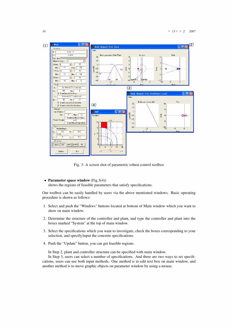
• Main window (Fig.3(1))has some edit field, controller, plant, specifications, and parameters.

• Control synthesis window (Fig.3(2))shows Bode diagram (for sensitivity function and complementary sensitivity function) andNyquist plot and Pole/Zero Location for closed-loop transfer function, and users change speci-fications to manipulate graphic objects on the control synthesis window.

• Open-loop window (Fig.3(3))shows Bode diagram and Pole/Zero Location for open-loop transfer function.

10 数式処理第 13巻第 2号 2007

Fig. 3: A screen shot of parametric robust control toolbox

• Parameter space window (Fig.3(4))shows the regions of feasible parameters that satisfy specifications.

Our toolbox can be easily handled by users via the above mentioned windows. Basic operatingprocedure is shown as follows:

1. Select and push the “Windiws" buttons located at bottom of Main window which you want toshow on main window.

2. Determine the structure of the controller and plant, and type the controller and plant into theboxes marked “System" at the top of main window.

3. Select the specifications which you want to investigate, check the boxes corresponding to yourselection, and specify/input the concrete specifications.

4. Push the “Update" button, you can get feasible regions.

In Step 2, plant and controller structure can be specified with main window.In Step 3, users can select a number of specifications. And there are two ways to set specifi-

cations, users can use both input methods. One method is to edit text box on main window, andanother method is to move graphic objects on parameter window by using a mouse.

J.JSSAC Vol. 13, No. 2, 2007 11

In Step 4, feasible regions are computed and shown on parameter region window. The tool-box shows feasible region which satisfy each specifications. Fig.3(4) is shown a superposition offeasible regions of sensitivity, complementary sensitivity and Hurwitz stability.

If users click or drag with the mouse on parameter region window, parameter values are re-flected in system, users can look see the behavior of bode and nyquist diagram and pole assignmenton parameter window.

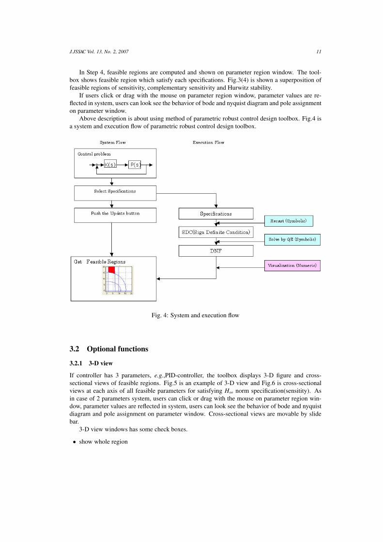
Above description is about using method of parametric robust control design toolbox. Fig.4 isa system and execution flow of parametric robust control design toolbox.

Fig. 4: System and execution flow

3.2 Optional functions

3.2.1 3-D view

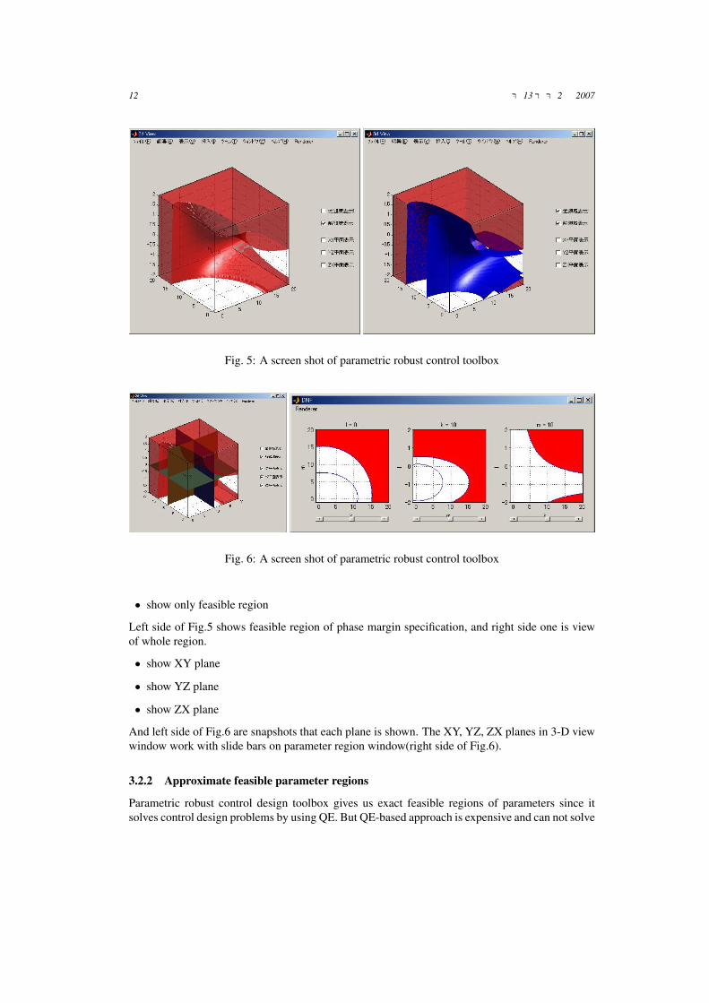
If controller has 3 parameters, e.g.,PID-controller, the toolbox displays 3-D figure and cross-sectional views of feasible regions. Fig.5 is an example of 3-D view and Fig.6 is cross-sectionalviews at each axis of all feasible parameters for satisfying H∞ norm specification(sensitity). Asin case of 2 parameters system, users can click or drag with the mouse on parameter region win-dow, parameter values are reflected in system, users can look see the behavior of bode and nyquistdiagram and pole assignment on parameter window. Cross-sectional views are movable by slidebar.

3-D view windows has some check boxes.

• show whole region

12 数式処理第 13巻第 2号 2007



• show only feasible region

Left side of Fig.5 shows feasible region of phase margin specification, and right side one is viewof whole region.

• show XY plane

• show YZ plane

• show ZX plane

And left side of Fig.6 are snapshots that each plane is shown. The XY, YZ, ZX planes in 3-D viewwindow work with slide bars on parameter region window(right side of Fig.6).

3.2.2 Approximate feasible parameter regions

Parametric robust control design toolbox gives us exact feasible regions of parameters since itsolves control design problems by using QE. But QE-based approach is expensive and can not solve

J.JSSAC Vol. 13, No. 2, 2007 13

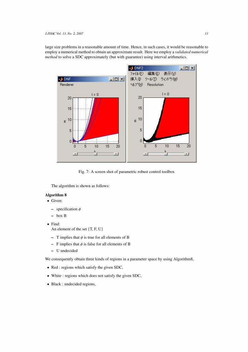
large size problems in a reasonable amount of time. Hence, in such cases, it would be reasonable toemploy a numerical method to obtain an approximate result. Here we employ a validated numericalmethod to solve a SDC approximately (but with guarantee) using interval arithmetics.


The algorithm is shown as follows:

Algorithm 8• Given:

– specification φ

– box B

• Find:An element of the set {T, F, U}

– T implies that φ is true for all elements of B

– F implies that φ is false for all elements of B

– U undecided

We consequently obtain three kinds of regions in a parameter space by using Algorithm8,

• Red : regions which satisfy the given SDC,

• White : regions which does not satisfy the given SDC,

• Black : undecided regions,

14 数式処理第 13巻第 2号 2007

which are composed by a set of boxes. One can first specify accuracy (fineness of a smallest box)when we use this function. In other words, this is a box decomposition of a parameter space withrespect to a given SDC to the specified accuracy. See the right side figure of Fig.7 for example.

4 ConclusionWe have been developing a parametric robust control design toolbox that is based on MATLAB andfor robust parametric control via a parameter space approach based on symbolic-numeric computa-tion. By using specialized QE, nonlinear and non-convex problems could be solved exactly, userscan get feasible parameter areas instead of feasible parameter point. This toolbox can treat not onlysingle objective problems but also multi-objective problems, we can check the feasible regions thatis superposed feasible regions of each problem. And our toolbox can be easily handled because thetoolbox is a GUI-based toolbox, and can show the feasible parameter areas by visualization. Forthose reason, this toolbox is very helpful in education and actual engineering fields.

5 AcknowledgmentsThis work has been supported in part by CREST of JST(Japan Science and Technology Agency).And I am deeply grateful to Mr.Myunghoon Hong, Mr.Hitoshi Yanami, Mr.Hirokazu Anai andProf. Shinji Hara for their cooperation.

A AppendixIn this section, we show the detailed usage of parametric robust control design toolbox.

A.1 How to use the toolbox

A.1.1 Basic function

Current version of parametric robust control design toolbox has four windows:

• Main window (Fig.8(1))has some edit field, controller, plant, specifications, and parameters.

• Control synthesis window (Fig.8(2))shows Bode diagram (for sensitivity function and complementary sensitivity function) andNyquist plot and Pole/Zero Location for closed-loop transfer function, and users change speci-fications to manipulate graphic objects on the control synthesis window.

• Open-loop window (Fig.8(3))shows Bode diagram and Pole/Zero Location for open-loop transfer function.

• Parameter space window (Fig.8(4))shows the regions of feasible parameters that satisfy spec-ifications.

Basic operating procedure is shown as follows:

J.JSSAC Vol. 13, No. 2, 2007 15

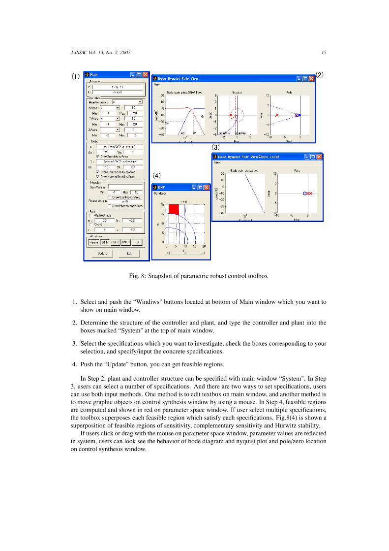
Fig. 8: Snapshot of parametric robust control toolbox

1. Select and push the “Windiws" buttons located at bottom of Main window which you want toshow on main window.

2. Determine the structure of the controller and plant, and type the controller and plant into theboxes marked “System" at the top of main window.

3. Select the specifications which you want to investigate, check the boxes corresponding to yourselection, and specify/input the concrete specifications.

4. Push the “Update" button, you can get feasible regions.

In Step 2, plant and controller structure can be specified with main window “System". In Step3, users can select a number of specifications. And there are two ways to set specifications, userscan use both input methods. One method is to edit textbox on main window, and another method isto move graphic objects on control synthesis window by using a mouse. In Step 4, feasible regionsare computed and shown in red on parameter space window. If user select multiple specifications,the toolbox superposes each feasible region which satisfy each specifications. Fig.8(4) is shown asuperposition of feasible regions of sensitivity, complementary sensitivity and Hurwitz stability.

If users click or drag with the mouse on parameter space window, parameter values are reflectedin system, users can look see the behavior of bode diagram and nyquist plot and pole/zero locationon control synthesis window.

16 数式処理第 13巻第 2号 2007

A.2 Description of window and how to use each window

A.2.1 Main window

Fig.8(1) is main window of parametric robust control toolbox. Users can do as follows on mainwindow.

• Input plant and controller functions.

• Select specifications.

• Select windows that users want look see.

A.2.2 System section

Fig. 9: System section

System section(Fig.9) is for inputting plant and controller functions. Users can use variable sand parameters k,m, l.

A.2.3 Variable section

Fig. 10: Variable section

Variable section(Fig.10) is for assign variables and parameter area, and show/assign parametervalues that are selected. This toolbox show feasible areas with k on x-axis, m on y-axis and l onz-axis.

1. Value of parameter k that is specified now on the parameter space window. This value is editableby not only keyboard input but also to click or drag on the parameter space window.

2. Minimum number of area of x-axis of parameter space window.

J.JSSAC Vol. 13, No. 2, 2007 17

3. Maximum number of area of x-axis of parameter space window.

4. Value of parameter m that is specified now on the parameter space window. This value iseditable by not only keyboard input but also to click or drag on the parameter space window.

5. Minimum number of area of y-axis of parameter space window.

6. Maximum number of area of y-axis of parameter space window.

7. Value of parameter l that is specified now on the parameter space window. This value is editableby not only keyboard input but also to click or drag on the parameter space window.

8. Minimum number of area of z-axis of parameter space window.

9. Maximum number of area of z-axis of parameter space window.

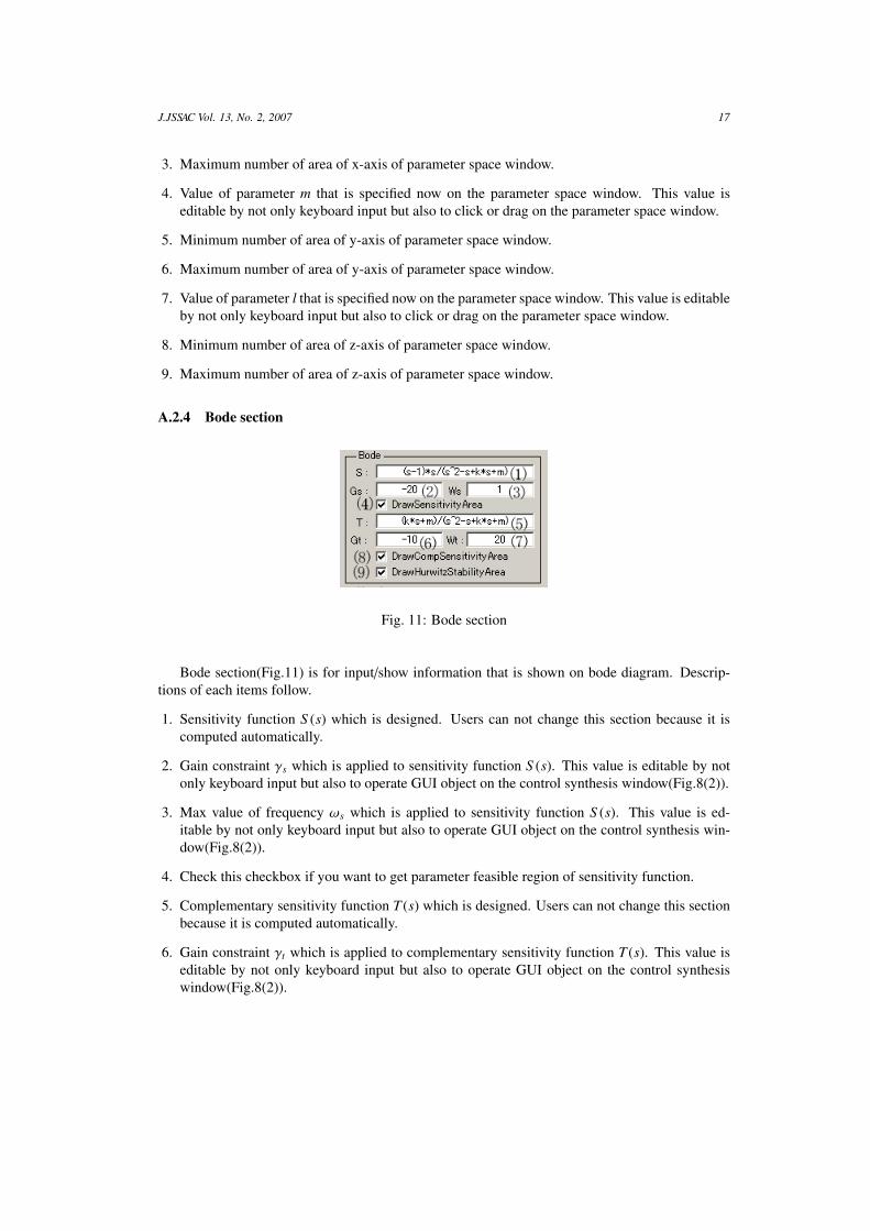
A.2.4 Bode section

Fig. 11: Bode section

Bode section(Fig.11) is for input/show information that is shown on bode diagram. Descrip-tions of each items follow.

1. Sensitivity function S (s) which is designed. Users can not change this section because it iscomputed automatically.

2. Gain constraint γs which is applied to sensitivity function S (s). This value is editable by notonly keyboard input but also to operate GUI object on the control synthesis window(Fig.8(2)).

3. Max value of frequency ωs which is applied to sensitivity function S (s). This value is ed-itable by not only keyboard input but also to operate GUI object on the control synthesis win-dow(Fig.8(2)).

4. Check this checkbox if you want to get parameter feasible region of sensitivity function.

5. Complementary sensitivity function T (s) which is designed. Users can not change this sectionbecause it is computed automatically.

6. Gain constraint γt which is applied to complementary sensitivity function T (s). This value iseditable by not only keyboard input but also to operate GUI object on the control synthesiswindow(Fig.8(2)).

18 数式処理第 13巻第 2号 2007

7. Minimum value of frequency ωt which is applied to complementary sensitivity function T (s).This value is editable by not only keyboard input but also to operate GUI object on the controlsynthesis window(Fig.8(2)).

8. Check this checkbox if you want to get parameter feasible region of complementary sensitivityfunction.

9. Check this checkbox if you want to get parameter feasible region of Hurwitz stability of controlsynthesis.

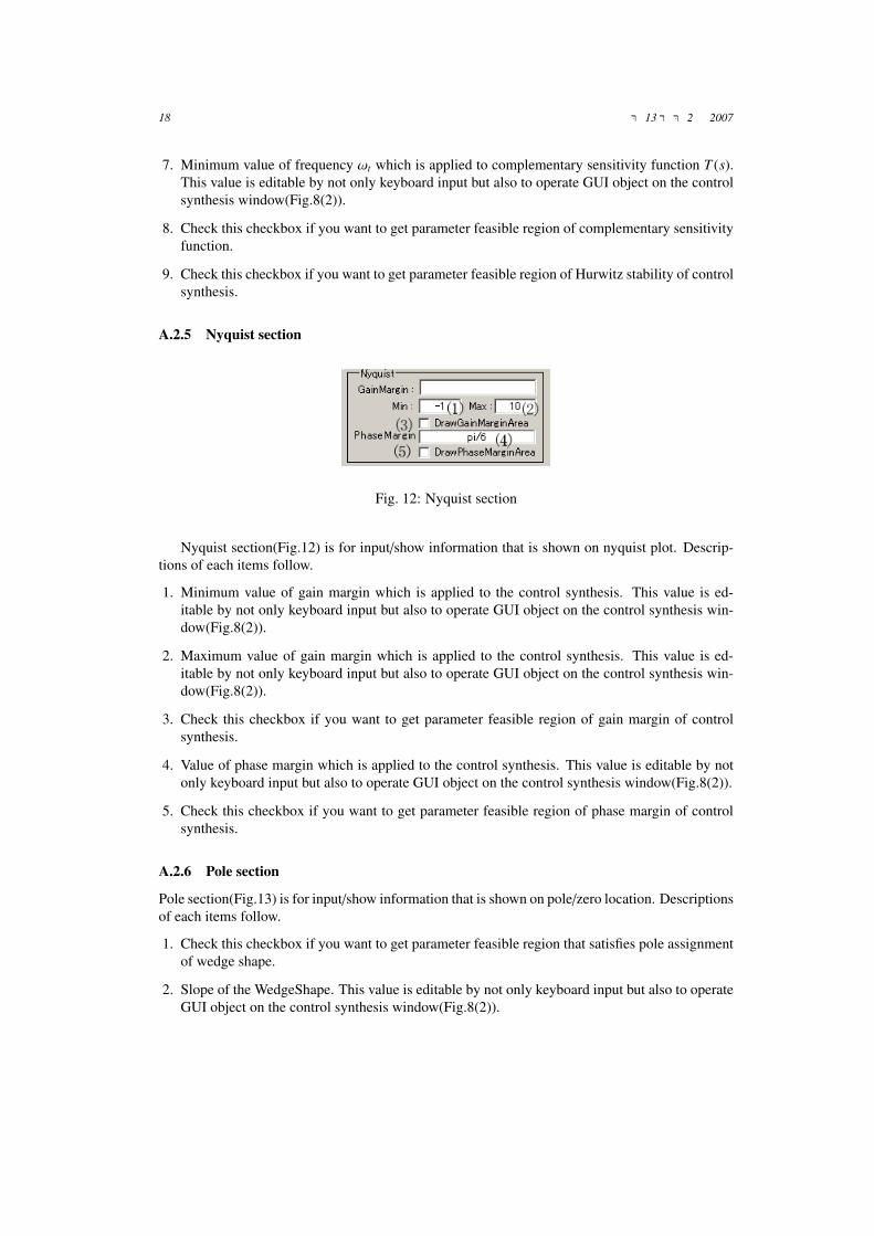
A.2.5 Nyquist section

Fig. 12: Nyquist section

Nyquist section(Fig.12) is for input/show information that is shown on nyquist plot. Descrip-tions of each items follow.

1. Minimum value of gain margin which is applied to the control synthesis. This value is ed-itable by not only keyboard input but also to operate GUI object on the control synthesis win-dow(Fig.8(2)).

2. Maximum value of gain margin which is applied to the control synthesis. This value is ed-itable by not only keyboard input but also to operate GUI object on the control synthesis win-dow(Fig.8(2)).

3. Check this checkbox if you want to get parameter feasible region of gain margin of controlsynthesis.

4. Value of phase margin which is applied to the control synthesis. This value is editable by notonly keyboard input but also to operate GUI object on the control synthesis window(Fig.8(2)).

5. Check this checkbox if you want to get parameter feasible region of phase margin of controlsynthesis.

A.2.6 Pole section

Pole section(Fig.13) is for input/show information that is shown on pole/zero location. Descriptionsof each items follow.

1. Check this checkbox if you want to get parameter feasible region that satisfies pole assignmentof wedge shape.

2. Slope of the WedgeShape. This value is editable by not only keyboard input but also to operateGUI object on the control synthesis window(Fig.8(2)).

J.JSSAC Vol. 13, No. 2, 2007 19

Fig. 13: Pole section

3. Distance from origin to WedgeShape. This value is editable by not only keyboard input butalso to operate GUI object on the control synthesis window(Fig.8(2)).

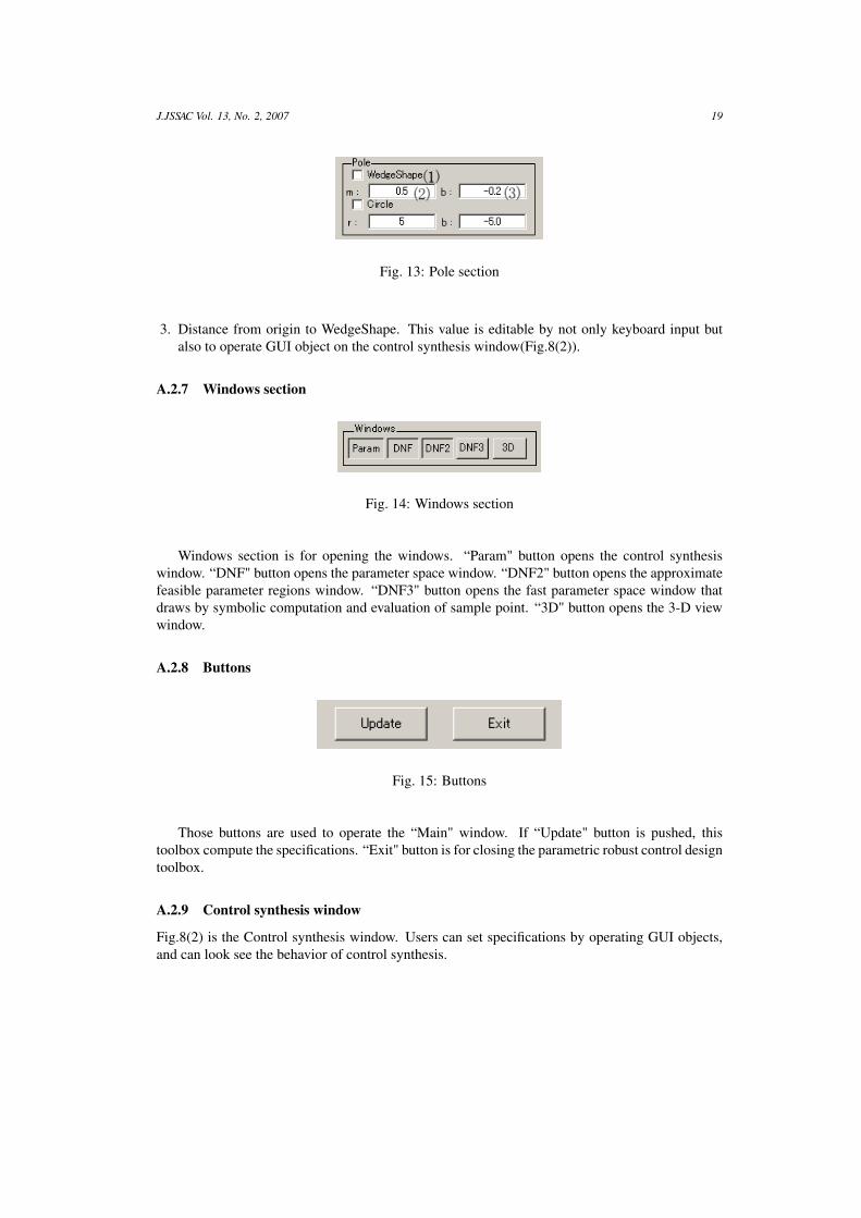
A.2.7 Windows section

Fig. 14: Windows section

Windows section is for opening the windows. “Param" button opens the control synthesiswindow. “DNF" button opens the parameter space window. “DNF2" button opens the approximatefeasible parameter regions window. “DNF3" button opens the fast parameter space window thatdraws by symbolic computation and evaluation of sample point. “3D" button opens the 3-D viewwindow.

A.2.8 Buttons

Fig. 15: Buttons

Those buttons are used to operate the “Main" window. If “Update" button is pushed, thistoolbox compute the specifications. “Exit" button is for closing the parametric robust control designtoolbox.

A.2.9 Control synthesis window

Fig.8(2) is the Control synthesis window. Users can set specifications by operating GUI objects,and can look see the behavior of control synthesis.

20 数式処理第 13巻第 2号 2007

A.2.10 Bode diagram

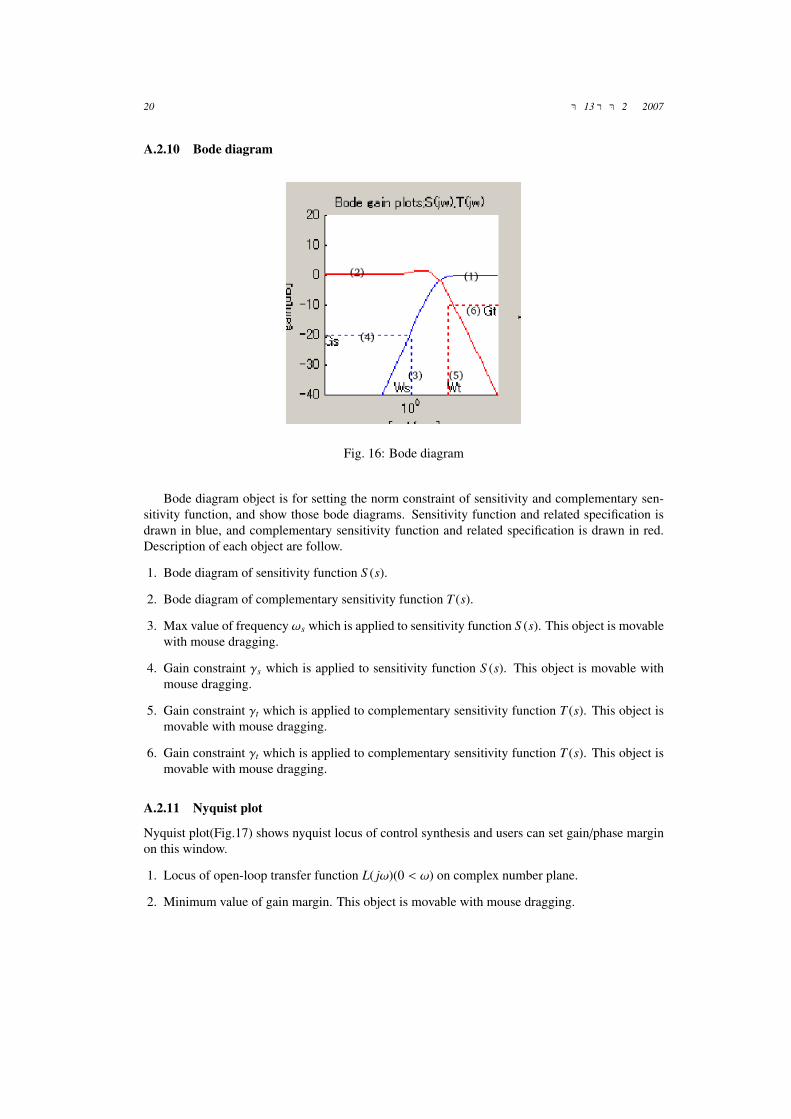
Fig. 16: Bode diagram

Bode diagram object is for setting the norm constraint of sensitivity and complementary sen-sitivity function, and show those bode diagrams. Sensitivity function and related specification isdrawn in blue, and complementary sensitivity function and related specification is drawn in red.Description of each object are follow.

1. Bode diagram of sensitivity function S (s).

2. Bode diagram of complementary sensitivity function T (s).

3. Max value of frequency ωs which is applied to sensitivity function S (s). This object is movablewith mouse dragging.

4. Gain constraint γs which is applied to sensitivity function S (s). This object is movable withmouse dragging.

5. Gain constraint γt which is applied to complementary sensitivity function T (s). This object ismovable with mouse dragging.

6. Gain constraint γt which is applied to complementary sensitivity function T (s). This object ismovable with mouse dragging.

A.2.11 Nyquist plot

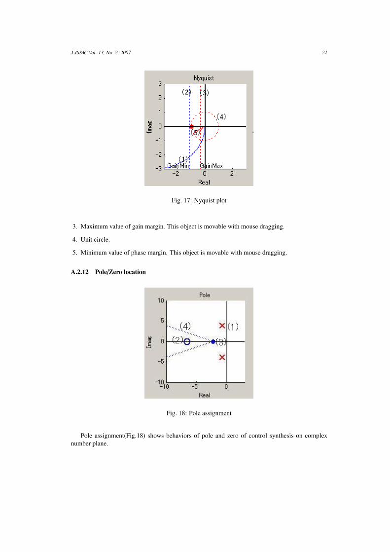
Nyquist plot(Fig.17) shows nyquist locus of control synthesis and users can set gain/phase marginon this window.

1. Locus of open-loop transfer function L( jω)(0 < ω) on complex number plane.

2. Minimum value of gain margin. This object is movable with mouse dragging.

J.JSSAC Vol. 13, No. 2, 2007 21

Fig. 17: Nyquist plot

3. Maximum value of gain margin. This object is movable with mouse dragging.

4. Unit circle.

5. Minimum value of phase margin. This object is movable with mouse dragging.

A.2.12 Pole/Zero location

Fig. 18: Pole assignment

Pole assignment(Fig.18) shows behaviors of pole and zero of control synthesis on complexnumber plane.

22 数式処理第 13巻第 2号 2007

1. Pole of control synthesis. If pole are in right half plane, control synthesis become unstable.

2. Zero of control synthesis. It negate pole of control synthesis.

3. Distance from origin to WedgeShape. This object is movable with mouse dragging.

4. Slope of the WedgeShape. This object is movable with mouse dragging.

A.2.13 Parameter space window

Parameter space window(Fig.19) shows feasible regions which satisfy the specifications that se-lected on the main window.

Fig. 19: Parameter space window

1. Border lines from specifications which are selected by user on main window.

2. Feasible parameter region which satisfy all selected specifications. This region colors in red.

3. Slide bar for changing parameter value which is interfaced with 3D view. This object is movablewith mouse clicking/dragging.

If users click or drag with the mouse on parameter region window, parameter values are reflectedin system, users can look see the behavior of control synthesis on control synthesis window.

J.JSSAC Vol. 13, No. 2, 2007 23

A.2.14 Optional functions

A.2.15 3-D view

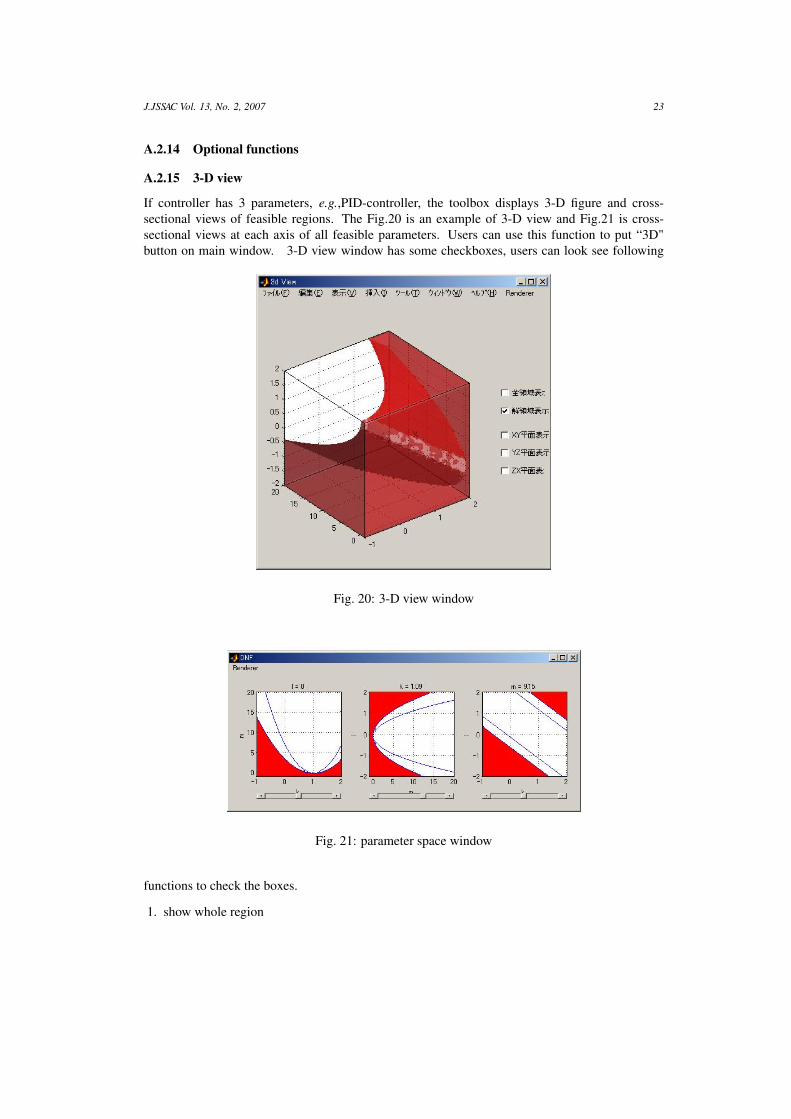
If controller has 3 parameters, e.g.,PID-controller, the toolbox displays 3-D figure and cross-sectional views of feasible regions. The Fig.20 is an example of 3-D view and Fig.21 is cross-sectional views at each axis of all feasible parameters. Users can use this function to put “3D"button on main window. 3-D view window has some checkboxes, users can look see following

Fig. 20: 3-D view window

Fig. 21: parameter space window

functions to check the boxes.

1. show whole region

24 数式処理第 13巻第 2号 2007

2. show only feasible region

3. show XY plane

4. show YZ plane

5. show ZX plane

And “Tools" which is menu of 3-D view window has some functions that operate 3-D objects,“Zoom in", “Zoom out", “3-D rotation", “Remove camera", etc. As in the case of 2 parameterssystem, users can click or drag with the mouse on parameter region window(right side of 20),parameter values are reflected in system, users can look see the behavior of bode and nyquistdiagram and pole assignment on parameter window. Cross-sectional views are movable by slidebar.

A.2.16 Approximate feasible parameter regions

Parametric robust control design toolbox us exact feasible regions of parameters since it solvescontrol design problems by using QE. But QE-based approach is expensive and can not solve largesize problems in a reasonable amount of time. Hence, in such cases, it would be reasonable toemploy a numerical method to obtain an approximate result. Here we employ a validated numericalmethod to solve a SDC approximately (but with guarantee) using interval arithmetics. Users canuse this function to put “DNF2" button on main window.

Fig. 22: Approximate feasible parameter regions

Users can select a drawing resolution “low", “mid", “high" from “Resolution" menu. Same asparameter space window, red area satisfy the selected specifications, and white area does not satisfythe selected specifications. The area that painted in black is unclear area that satisfy or not satisfythe specification under selected resolution. And the function that users can look see the behaviorof control synthesis is not implemented in this function.

J.JSSAC Vol. 13, No. 2, 2007 25

References[1] H. Anai and S. Hara. Fixed-structure robust controller synthesis based on sign definite con-

dition by a special quantifier elimination. In Proceedings of American Control Conference2000, pages 1312–1316, 2000.

[2] H. Anai, H. Yanami, K. Sakabe, and S. Hara, “Fixed-structure robust controller synthesisbased on symbolic-numeric computation: design and algorithms with a CACSD toolbox,”Proceedings of CCA/ISIC/CACSD 2004 (Taipei, Taiwan), pp 1540–1545, 2004.

[3] L. Gonzàlez, H. Lombardi, T. Recio, and M.-F. Roy. Sturm-Habicht sequence. In Proceedingsof the ACM SIGSAM 1989 International Symposium on Symbolic and Algebraic Computation,pages 136–146. ACM-Press, 1989.

[4] L. González-Vega, T. Recio, H. Lombardi, and M.-F. Roy. Sturm-Habicht sequences deter-minants and real roots of univariate polynomials. In B.F. Caviness and J.R. Johnson, editors,Quantifier Elimination and Cylindrical Algebraic Decomposition, Texts and Monographs inSymbolic Computation, pages 300–316. Springer, Wien, New York, 1998.

[5] K. Sakabe, H. Yanami, H. Anai and S. Hara, “MATLAB toolbox for robust control synthesisby symbolic computation” Proceedings of SICE Annual Conference 2004 (Sapporo, Japan),pp. 1968–1973, 2004.

[6] S.Hara, T.Kimura and R.Kondo, “Parameter space design for H∞ control(in Japanese),” Trans.of SICE, vol.27,no.6,pp. 714–716, 1991.

[7] S.Hara, T.Kimura and R.Kondo. “H∞ control system design by a parameter space approach”In Proceedings of MTNS-91(Koube, Japan), pp. 287–292, 1991.

[8] T.Kimura and S.Hara. “A Robust Control System Design by a Parameter Space ApproachBased on Sign Definite Condition” In Proceedings of Korean Automatic Control Confer-ence(KACC), pp. 1533–1538, 1991.

[9] H.Anai and H.Yanami. “SyNRAC: A Maple-package for solving real algebraic constraints”In Proceedings of International Workshop on Computer Algebra Systems and their Applica-tions(CASA) 2003 (Saint Petersburg, Russian Federation), P.M.A. Sloot et al. (Eds.):ICCS2003, LNCS2657.Springer, pp. 828–837, 2003.

[10] Noriko Hyodo, Myunghoon Hong, Hitoshi Yanami, Hirokazu Anai, Shinji Hara. “Develop-ment of a MATLAB toolbox for parametric robust control — new algorithms and functions—” In Proceedings of SICE Annual Conference 2006 (Busan, Korea), pp. 2856–2861, 2006.

development of parametric robust control design … 数式処理第13 巻第2 号2007 control...

Documents