engineering physics laboratory … manuals phy-10… · engineering physics laboratory engineering...
TRANSCRIPT
ENGINEERING PHYSICS LABORATORY ENGINEERING PHYSICS LABORATORY ENGINEERING PHYSICS LABORATORY ENGINEERING PHYSICS LABORATORY
EXPERIMENTSEXPERIMENTSEXPERIMENTSEXPERIMENTS MANUALMANUALMANUALMANUAL
CONTENTS:
Instruction for Laboratory ……3
Experiment 1: Measurement of basic constants: Length, Weight & Time. ……4
Experiment 2: To study Newton’s Law (1st, 2nd and 3rd Law). .....11
Experiment 3: Current balance/ force acting on a current carrying …..22
Conductor.
Experiment 4: Magnetic field of paired coils in a Helmholtz arrangement. …..25
Experiment 5: Interference & diffraction of Light by Slits. …..31
Experiment 6: Interference by Fresnel’s biprism. .….37
Experiment 7: Cauchy’s constant using Prism. .….41
Experiment 8: To find wavelength of white light by using Plane
Transmission Diffraction Grating. …..46
Experiment 9: Polarization (Malus’s Law) …..52
Experiment 10: Electron Diffraction (Dual nature of Electron) …..57
Experiment 11: Photoelectric effect (Plank’s Constant) …..62
Experiment 12: Coupled Pendulum …..71

Page 2
INSTRUCTION FOR LABORATORY Specific Instructions 1. Assessment in the course is based on (i) Your performance in the laboratory class (ii) Your laboratory report and (iii) The end-semester examination. The Physics laboratory course will be done as follows:
Internal assessment (50 Marks) Examination (50 Marks) Experiment performance
Internal viva Others Experiment performance
Examination viva
30 15 5 30 20 2. A prior study about the experiment is essential for good performance in the class. Read the instruction manual carefully before coming to the lab class. If you come unprepared to the lab; your performance would be accordingly affected. 3. You are expected to perform the experiment, complete the calculations and data analysis, and submit the report of every experiment on the same day within the laboratory slot assigned for it. 4. You must bring with you the following material to the lab: report sheets pen, pencil, small scale, instruction manual, graph sheets, calculator and a file cover and any other stationary item required. The PENCIL is to be used only for graph. Data should be recorded with the PEN. 5 At least one set of observation should be signed by the faculty / instructor. An unsigned observation data will be awarded ZERO. 6. It is important to estimate the maximum possible error of the results using the given Apparatus/data. 7. Each graph should be well documented; abscissa and ordinate along with the units should be mentioned clearly. The title of the graph should be stated on the top of each graph paper. 8. You are expected to give a careful thought on the precautions to be observed in handling any equipment and conducting the experiment. In case of any doubt you should feel free to interact with the instructors. 9. Report must be prepared in the following format: (i) Name, Roll No., lab group, date of experiment. (ii) Objective of the experiment, working formula only , meaning of symbols and the Schematic diagram of the experimental setup. 10. Other Required equipments (e.g., Spectral filter etc.) will be issued prior to the experiment. The students are supposed to return the equipments on the same day after the completion of the experiment.

Page 3
EXPERIMENT 1:
MEASUREMENT OF BASIC CONSTANTS: LENGTH, WEIGHT AND TIME
OBJECT: 1. Determination of the volume of tubes with the caliper gauge. 2. Determination of the thickness of wires cubes and plates with the micrometer. 3. Determination of the thickness of plates and the radius of curvature of watch glasses with the spherometer. 4. Determination of the weight of different articles with highest possible accuracy with a manual precision balance. 5. Determination of the frequency and time period of the pendulum. PRINCIPLE AND TASK: Caliper gauges, micrometers and spherometers are used for the accurate measurement of lengths, thicknesses, diameters and curvatures. A mechanical balance is used for weight determinations; a decade counter is used for accurate time measurements. Measuring procedures, accuracy of measurement and reading accuracy are demonstrated.
Fig. 1: Experimental set-up: Measurement of basic constants: length, weight, and time
Page 4
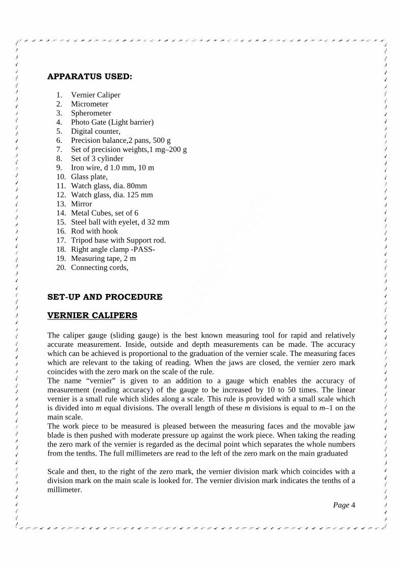
APPARATUS USED:
1. Vernier Caliper 2. Micrometer 3. Spherometer 4. Photo Gate (Light barrier) 5. Digital counter, 6. Precision balance,2 pans, 500 g 7. Set of precision weights,1 mg–200 g 8. Set of 3 cylinder 9. Iron wire, d 1.0 mm, 10 m 10. Glass plate, 11. Watch glass, dia. 80mm 12. Watch glass, dia. 125 mm 13. Mirror 14. Metal Cubes, set of 6 15. Steel ball with eyelet, d 32 mm 16. Rod with hook 17. Tripod base with Support rod. 18. Right angle clamp -PASS- 19. Measuring tape, 2 m 20. Connecting cords,
SET-UP AND PROCEDURE VERNIER CALIPERS
The caliper gauge (sliding gauge) is the best known measuring tool for rapid and relatively accurate measurement. Inside, outside and depth measurements can be made. The accuracy which can be achieved is proportional to the graduation of the vernier scale. The measuring faces which are relevant to the taking of reading. When the jaws are closed, the vernier zero mark coincides with the zero mark on the scale of the rule. The name “vernier” is given to an addition to a gauge which enables the accuracy of measurement (reading accuracy) of the gauge to be increased by 10 to 50 times. The linear vernier is a small rule which slides along a scale. This rule is provided with a small scale which is divided into m equal divisions. The overall length of these m divisions is equal to m–1 on the main scale. The work piece to be measured is pleased between the measuring faces and the movable jaw blade is then pushed with moderate pressure up against the work piece. When taking the reading the zero mark of the vernier is regarded as the decimal point which separates the whole numbers from the tenths. The full millimeters are read to the left of the zero mark on the main graduated Scale and then, to the right of the zero mark, the vernier division mark which coincides with a division mark on the main scale is looked for. The vernier division mark indicates the tenths of a millimeter.
Page 5
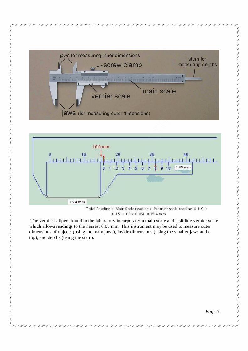
The vernier calipers found in the laboratory incorporates a main scale and a sliding vernier scale which allows readings to the nearest 0.05 mm. This instrument may be used to measure outer dimensions of objects (using the main jaws), inside dimensions (using the smaller jaws at the top), and depths (using the stem).

Page 6
MICROMETER SCREW GAUGE The micrometer screw gauge is used to measure even smaller dimensions than the vernier calipers. The micrometer screw gauge also uses an auxiliary scale (measuring hundredths of a millimeter) which is marked on a rotary thimble. Basically it is a screw with an accurately constant pitch (the amount by which the thimble moves forward or backward for one complete revolution). The micrometers in our laboratory have a pitch of 0.50 mm (two full turns are required to close the jaws by 1.00 mm). The rotating thimble is subdivided into 50 equal divisions. The thimble passes through a frame that carries a millimeter scale graduated to 0.5 mm. The jaws can be adjusted by rotating the thimble using the small ratchet knob. This includes a friction clutch which prevents too much tension being applied. The thimble must be rotated through two revolutions to open the jaws by 1 mm.
In order to measure an object, the object is placed between the jaws and the thimble is rotated using the ratchet until the object is secured. Note that the ratchet knob must be used to secure the object firmly between the jaws, otherwise the instrument could be damaged or give an inconsistent reading. The manufacturer recommends 3 clicks of the ratchet before taking the reading. The lock may be used to ensure that the thimble does not rotate while you take the reading.
The first significant figure is taken from the last graduation showing on the sleeve directly to the left of the revolving thimble. Note that an additional half scale division (0.5 mm) must be included if the mark below the main scale is visible between the thimble and the main scale division on the sleeve. The remaining two significant figures (hundredths of a millimeter) are taken directly from the thimble opposite the main scale.
The reading is 7.38 mm

Page 7
NOTE: Taking a zero reading
Whenever you use a vernier calipers or a micrometer screw gauge you must always take a zero reading i.e. a reading with the instrument closed. This is because when you close your calipers, you will see that very often (not always) it does not read zero. Only then open the jaws and place the object to be measured firmly between the jaws and take the open reading. Your actual measurement will then be the difference between your open reading and your zero reading.
SPHEROMETER
BASIC PRINCIPLES The spherometer consists of a tripod with three steel legs that tap er into points forming the vertices of an equilateral triangle, each side of which measures 50 mm. A micrometer screw with a pointed tip passes through the centre of the tripod. A vertical scale shows the height h of the micrometer tip above or below the surface on which the legs of the spherometer rest. The displacement of the micrometer tip can be read to a precision of 1µm using a Vernier scale on a disc that rotates along with the micrometer screw.
The relation between the distance of the legs from the centre of the spherometer a, the unknown radius of curvature R and the height of curvature h is given by the equation:
R2 = r2 + (R-h)2 From the above equation, the value of R can be determined by transposition: R = (r2 +h2) / 2.h The value for the distance r can be calculated from the length s which is the length of each side of the equilateral triangle formed by the legs of the spherometer: r = s / √3 The equation for determine R is as follows: R = s2/ 6.h + h/2

Page 8
DIGITAL COUNTER
The electronic counter / timer is able to measure time, frequencies, rates and periods as well as counting events or pulses from a Geiger tube. When counting events, it is possible to set certain fixed periods of time for the count. In addition, an arbitrary time period anywhere between 1s and 99999s can be programmed. Counting can be triggered (started or stopped) either by a signal to the input terminals or manually by means of a switch. OPERATION:
1. Time measurement (Time that a light barrier is obscured)
• Connect socket out start and in stop together using experiment leads. • Connect a light barrier (Photo gate) to socket A.
The period to be measured is the length of time that a moving body takes to move through the light beam (Photo gate). Its entry into the beam obscures the receptor and starts the timer. When body exits the beam the receptor detects the light again and the timer is stopped.
2. Periods of a Pendulum
• Set the selector to the symbol pendulum TA.
• Apply an input signal to terminal or connect a light barrier (Photo gate) to socket A.
The time to be measured is the number of milliseconds between successive low to high (L/H) edges detected at terminal or three interruptions to the light beam detected at terminal A.

Page 9
3. Counting Periods
Fixed Periods: • Set the selector switch to the desired period (NA1/10/60s). • Apply an input signal to terminal instartcount or connect a photo gate to terminal
A.
• Start counting by pressing the start button.
The equipment counts L/H edges at terminal pulses from a Geiger tube connected to terminal or interruptions to a light barrier connected to terminal A.
Programmable Time Periods:
• Set the selector switch to the symbol NA (hand).
• Press the start button to set tens, hundreds, thousands or ten thousands of seconds (incremented by pressing the button).
• The stop has a similar effect but causes the times to be decremented.
• Confirm the period by pressing Reset. The display will flash briefly then reset to 0.
• Pressing start activates the counter input and gate led lights, indicating readiness to count.
4. Frequency Measurement • Set the selector to fA (HZ or kHZ).
• Apply an input signal to terminal IN STRATCOUNT. • Start measurement by pressing start. The gate led lights indicating readiness to
count.

Page 10
EXPERIMENT 2 (A):
NEWTON’S 1st LAW AIM/ OBJECT: To study the Newton’s first law “An object at rest will remain at rest. An object in motion will remain in motion”. APPARATUS USED:
1. PAS car Dynamics System 2. Motion Sensor 3. Hover Puck 4. Discover Friction Accessory 5. Physics String 6. Computer Interface 7. Science Workshop
INTRODUCTION: The purpose of this experiment is to determine how external forces influence an object's motion. The following objects are pushed briefly: a Hover Puck, a Cart and a Friction Tray. The resulting velocity is measured with a Motion Sensor. An analysis of this motion yields Newton's 1st Law. THEORY: Students may be familiar with the following definition of inertia - also know as Newton's 1st Law: "An object at rest will remain at rest. An object in motion will remain in motion." However, how does a scientist quantify the statement above? Specifically, what affects the object's speed and direction? These are all questions best left for direct investigation... SET-UP for Science Workshop Sensors
Page 11
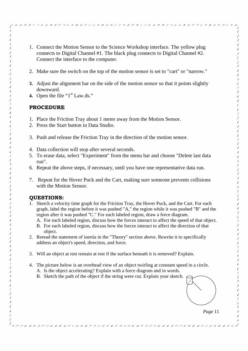
1. Connect the Motion Sensor to the Science Workshop interface. The yellow plug connects to Digital Channel #1. The black plug connects to Digital Channel #2. Connect the interface to the computer.
2. Make sure the switch on the top of the motion sensor is set to "cart" or "narrow." 3. Adjust the alignment bar on the side of the motion sensor so that it points slightly
downward. 4. Open the file “1st Law.ds.” PROCEDURE 1. Place the Friction Tray about 1 meter away from the Motion Sensor. 2. Press the Start button in Data Studio.
3. Push and release the Friction Tray in the direction of the motion sensor.
4. Data collection will stop after several seconds. 5. To erase data, select "Experiment" from the menu bar and choose "Delete last data
run". 6. Repeat the above steps, if necessary, until you have one representative data run.
7. Repeat for the Hover Puck and the Cart, making sure someone prevents collisions
with the Motion Sensor. QUESTIONS: 1. Sketch a velocity time graph for the Friction Tray, the Hover Puck, and the Cart. For each
graph, label the region before it was pushed "A," the region while it was pushed "B" and the region after it was pushed "C." For each labeled region, draw a force diagram. A. For each labeled region, discuss how the forces interact to affect the speed of that object. B. For each labeled region, discuss how the forces interact to affect the direction of that
object. 2. Reread the statement of inertia in the "Theory" section above. Rewrite it to specifically
address an object's speed, direction, and force. 3. Will an object at rest remain at rest if the surface beneath it is removed? Explain.
4. The picture below is an overhead view of an object twirling at constant speed in a circle.
A. Is the object accelerating? Explain with a force diagram and in words. B. Sketch the path of the object if the string were cut. Explain your sketch.
Page 12
EXPERIMENT 2 (B):
NEWTON’S 2ND LAW
AIM/ OBJECT: To study the Newton’s second law “F = ma”. APPARATUS USED:
1. PAS car Dynamics System 2. Motion Sensor 3. Force Sensor 4. Smart Pulley with Clamp 5. Mass and Hanger Set 6. Physics String 7. Adjustable Feet (Optional) 8. Computer Interface 9. Science Workshop
INTRODUCTION The purpose of this experiment is to determine Newton’s 2nd Law. A modified version of Atwood’s machine is set up with a mass tied to string that hangs over a pulley at the end of a table. The other end of the string is tied to a Force Sensor mounted on a cart. A Motion Sensor records the velocity of the cart. THEORY
The acceleration a of a body is parallel and directly proportional to the net force F acting on the body, is in the direction of the net force, and is inversely proportional to the mass m of the body, i.e., F = ma.
The following equation is Newton’s 2nd Law: Σ F = ma F represents the forces acting upon a mass, m; and a represents the resulting acceleration. Imagine an object in space pulled in opposite directions by two equal forces. The sum of these forces, therefore, equals zero. According to Newton’s 2nd Law, the mass will not accelerate. If, however, the forces are not equal, then the object will accelerate in the same direction as the net force.

Page 13
In this lab, the acceleration must be measured from a velocity-time graph. Since acceleration is defined as the change in the velocity per unit time, then the slope of the velocity-time graph equals the acceleration. Flat Track with Hanging Mass In this lab exercise, a cart is attached by a piece of string to another mass which is hung over the table supporting the cart track by a pulley so that as the hanging mass falls, it pulls the cart along the track. For this kind of problem, it is useful to draw a diagram of the forces acting on each of the masses involved in the problem. The experimental setup is shown in Figure. The forces acting on the cart and hanging mass are labelled in Figure. Free-body diagrams of the forces on the cart and hanging mass are provided.
Figure: Forces on Dynamics Cart with Hanging Mass

Page 14
Since force is a vector quantity, it is necessary to decide what are the positive and negative directions so that each force can be labeled as being either positive or negative. A useful rule is to say that the direction of motion is the positive direction. This direction is indicated in both Figures 1 and 2. With this convention in place, equations for the total force acting on each object can be written down. For the cart, this equation is,
ΣFcartx = T = MC aC In this equation, Fcartx is the total force on the cart in the horizontal, or x, direction, T is the tension in the string, which always pulls away from the mass in the direction of the string, MC is the mass of the dynamics cart, and aC is the acceleration of the cart in the horizontal direction. Since we do not expect the cart to lift o® of the air track or collapse into the track, we can say that there is no net force acting in the vertical, or y, direction. This means that the normal force, n, must be balanced by the weight of the cart, Mcg, so that n = Mcg. To solve for the acceleration of the cart, from Equation 2, we need to know the tension in the string, T. To obtain the tension in the string, consider the forces acting on the hanging mass. From the forces illustrated in Figure 2, the following equation can be written down using Newton's second law, ΣFH = mH g - T = mH aH: In this equation, all of the variables have the same meaning with the addition that FH is the total force on the hanging weight, mH is the mass of the hanging weight, and aH is the acceleration of the hanging weight. Since both the hanging mass and the dynamics cart are connected by the same piece of string, which is assumed not to stretch, the same tension acts on both. This tension is responsible for accelerating the cart. For the tension to be the same on both the dynamics cart and on the hanging mass, the acceleration of each must also be the same. To demonstrate that this is correct, consider what would happen if the acceleration was not the same for both. For example, if the dynamics cart was to accelerate progressively faster than the hanging mass, then the string would go limp resulting in no tension in the string. If the hanging mass was to accelerate progressively faster than the dynamics cart, then the string would snap maximizing the hanger's fall due to gravity. Since the string connecting the two neither loosens nor breaks, the tension acting on each object must be the same, and the acceleration of each mass must also be the same. This will be examined during the lab exercise. The variable for tension, T is used in both equations 2 and 3 indicating a certain understanding of tension acting on both the cart and hanging mass. Since the acceleration is the same for both, the two accelerations, aC and aH, can be replaced by a single variable for the acceleration, a. Equations 2 and 3 can be rewritten as, Mca = T;
mHa = mHg – T Substituting the tension T in Equation 5 with the tension T from Equation 4, and solving for the acceleration (which is the same for both the hanging mass and the cart) gives,

Page 15
SET-UP for Science Workshop Sensors
1. Connect the Motion Sensor to the Science Workshop interface. The yellow plug connects to
Digital Channel #1. The black plug connects to Digital Channel #2. Make sure the switch on the top of the motion sensor is set to "cart" or "narrow."
2. Connect the Force Sensor to Analog Channel #A. Connect the interface to the computer. 3. Using the long thumbscrew, attach the Force Sensor to the cart. 4. Place the Motion Sensor on one end of the track as in the picture above. Adjust the alignment
knob on the side of the motion sensor so that it points parallel to the track. 5. Level the track. 6. Optional: Use adjustable feet on both ends to level the track.
Attach the Motion Sensor to the end of the track as shown at right.
7. Clamp the pulley to the other end of the track. Place this end over
the edge of the table. 8. Wrap one end of a one meter length of string around the notch of the mass hanger. 9. Place the Cart/Force Sensor assembly on the track. Tie the other end of the string to the hook
of the Force Sensor. Hang the mass hanger over the pulley. 10. Level the string by adjusting the pulley. 11. Open the file “2nd Law.ds.”

Page 16
PROCEDURE 1. With no tension on the string, press the "TARE" or "ZERO" button on the Force Sensor. 2. Pull the cart back as far as possible without allowing the mass hanger to contact the pulley. 3. Simultaneously press the START button at the top of Data Studio and release the cart.
Prevent the cart from colliding with the pulley. 4. Make sure the Force Sensor’s cord does not impede the cart’s motion. 5. Data recording will stop automatically. 6. Using the cursor, highlight only the section of the velocity graph that corresponds to the
intended motion. Press the Fit button and select “Linear Fit.” Enter the value of the acceleration into the data table.
7. Using the cursor, highlight only the section of the force graph that corresponds to the accelerated motion. The legend displays the mean force for this highlighted section. Enter the value of the mean force into the data table.
8. Go to the EXPERIMENT menu and select "Delete all Data Runs." 9. Repeat the previous steps until a total of 4 data runs are collected. Each time increase the
mass by 5 grams. 10. Observe the Force v Acceleration graph. Press the Fit button and select “Linear Fit.” Record
the values of the slope and vertical intercept. 11. Find the mass in kilograms of the Cart and Force Sensor. OBSERVATION TABLE: S.No. Mass (m) Used
for generate Force
Calculated Force (m X g) in Newton’s
Measured Force ( F) in Newton’s
Measured Acceleration a (dv/dt) m/s2
% Error
1. 05gm 2. 10gm 3. 15gm 4. 20gm 5. 25gm 6. 30gm 7. 35gm 8. 40gm 9. 45gm 10. 50gm

Page 17
DATA PROCESSING
Plot a graph between Measured Force F and acceleration a. and its compare with the calculated force and acceleration graph.
ANALYSIS What is the nature of the relationship between these two variables? What does this tell us about how changes in the acceleration will affect the force acting on a car? QUESTIONS 1. What physical property does the slope of the Force vs Acceleration graph represent? Explain.
2. What physical property does the vertical intercept represent?
3. Write a linear equation for the Force v Acceleration graph.
4. In your linear equation, would you expect the vertical intercept to equal zero? Explain.
5. Draw a force diagram of the cart as it moves down the track. What can be said about the sum of the forces on the cart? What can be said of the motion of the cart?

Page 18
EXPERIMENT 2 (C):
NEWTON'S 3RD LAW
AIM/ OBJECT: To study the Newton’s third law "For every action there is an equal and opposite reaction." APPARATUS USED:
1 PAS car Dynamics System 2 Force Sensor 3 Computer Interface 4 Data Studio Software
INTRODUCTION The purpose of this experiment is to determine the relationship between interacting forces. Two Force Sensors are used to measure the paired forces in a rubber band tug-o-war and the paired forces in a collision of two carts. THEORY Students may be familiar with the following definition of Newton's 3rd Law: When two bodies interact by exerting force on each other, these action and reaction forces are equal in magnitude, but opposite in direction. "For every action there is an equal and opposite reaction." However, how does the statement above manifest itself in physical interactions? Specifically, what determines the magnitude and direction of the forces? These are all questions best left for direct investigation... Part 1 SET-UP for Science Workshop Sensors
1. Connect one Force Sensor to analog channel A of the Science Workshop interface. Connect
the other Force Sensor to analog channel B. Connect the interface to the computer. 2. With nothing connected to the Force Sensors, press the "ZERO" or "TARE" buttons on the
Force Sensors. 3. Attach the hooks of the Force Sensors to the ends of a long rubber band as in the picture
above. 4. Open the file “3rd Law Tug-O-War.ds.”

Page 19
PART 1 PROCEDURE
1. Press the Start button in Data Studio. 2. Play a small-scale game of tug-o-war with neither Person A nor Person B winning.
3. Data Collection will end after several seconds.
4. If necessary to delete unwanted data, click the "Experiment" button and select "Delete all
data runs."
5. Record the direction and magnitude of the: A. Force of person A on Person B (FAB) B. Force of person B on Person A (FBA)
6. Repeat steps 1-5 above with Person A winning. 7. Repeat steps 1-5 above with Person B winning.
Part 2 SET-UP for Science Workshop Sensors
1. Remove the hooks from the Force Sensors. Replace them with the rubber bumpers. 2. Using long thumbscrews, attach the Force Sensors to the carts as in the picture above. Place
the carts on the track. 3. With nothing connected to the Force Sensors, press the "ZERO" or "TARE" buttons on the
Force Sensors. 4. Open the file “3rd Law Collision.ds.”

Page 20
Part 2 Procedure 1. Place an extra mass on one of the carts such that its mass is at least double that of the other
cart. 2. Place the more massive cart stationary in the middle of the track.
3. Press the Start button in Data Studio. 4. With the rubber bumpers facing each other, briefly and gently push the other cart into the
stationary cart. 5. Data collection will end after several seconds. 6. If necessary to delete unwanted data, click on the "Experiment" menu and select "Delete all
data runs." 7. Record the direction and magnitude of the forces. 8. Remove the extra mass and repeat the procedures above. QUESTIONS 1. Review the force-time graphs from Part 1. Draw force diagrams for each sensor. For the
force of sensor "A" on sensor "B," use the label "FAB." For the force of sensor "B" on sensor "A," use the label "FBA."
2. Write a statement that relates the two forces in Part 1. Make sure your statement includes the direction of the forces.
3. Review the force-time graphs from Part 2. Draw force diagrams for each sensor. For the
force of sensor "A" on sensor "B," use the label "FAB." For the force of sensor "B" on sensor "A," use the label "FBA."
4. Write a statement that relates the two forces in Part 2. Make sure your statement includes the
direction of the forces. 5. The relationships observed in this lab involved forces in contact with each other. Would the
statements you developed in questions 2 and 4 still apply to paired forces not in contact with each other? Explain. Hint: Imagine an apple falling to the earth. Draw force diagrams for the apple and the earth.
A large vehicle collides with a small ball. Which object experiences the greater force? Draw force diagrams for each and explain.

Page 21
EXPERIMENT 3: CURRENT BALANCE
AIM / OBJECT: To study the force acting on a current carrying conductor in a magnetic field and verify the Lorentz equation F= I (L X B). APPARATUS USED:
1 Power Supply 0-24V AC/DC 2 Cent –o-Gram Balance 3 Magnet (6Pc) 4 Different length Wires (Set of 6) 5 Pan With Pan Bow 6 Pan Support 7 Connecting Cords
INTRODUCTION A current carrying wire in a magnetic field experiences a force that is usually referred to as a magnetic force. The magnitude and direction of this force depend on four variables:
(i) The magnitude of the current(I) (ii) The length of wire (L) (iii)The strength of the magnetic field (B) and (iv) The angle between the field and the wire (Ө).
This magnetic force can be described mathematically by the vector cross product:
F= I (L X B) Or in scalar terms F = ILB Sin Ө

Page 22
1: FORCE VERSUS CURRENT PROCEDURE:
1. Set up the apparatus. 2. Determine the mass of the magnet holder and magnets with no current flowing. Record
this value in the column under Mass in table format. 3. Set the current to 0.5Amp. Determine the new mass of the magnet assembly. Record this
value under mass. 4. Subtract the mass value with the current flowing from the value with no current flowing.
Record this difference as the force. 5. Increase the current in 0.5amp increments to a maximum of 0.5amp, each time repeating
steps 2-4. DATA PROCESSING
Plot a graph of Force (vertical axis) vs Current (horizontal axis). ANALYSIS What is the nature of the relationship between these two variables? What does this tell us about how changes in the current will affect the force acting on a wire that is inside a magnetic field? OBSERVATION:
Current I (amps)
Mass m1 (gram)
Mass m2 (gram)
Change in Mass (∆M= m2-m1)
Force F = (∆m X g) in Newton’s
0.0 0.5 1.0 1.5 2.0 2.5 3.0 3.5 4.0 4.5 5.0
Note: 1. we use balance readings in grams, if we use actual force simply multiply grams by 0.0098 Newton/gm in Newton’s or by 980 dyne/gm in dynes.
2. The Lorentz Force is applied to an electric charge that moves through a magnetic field. It
is perpendicular to the direction of the charge and the direction of the magnetic field. The direction of the force is demonstrated by the Right Hand Rule.

Page 23
2: FORCE VERSUS LENGTH OF WIRE PROCEDURE:
1. Set up the apparatus. 2. Determine the length of the conductive foil on the current Loop. Record this value in the
column under Length in table format. 3. With no current flowing, determine the mass of the magnet assembly. Record this value
on the line at the top of the table. 4. Set the current to 2.0 amps. Determine the new mass of the magnet assembly. Record
this value under mass in table. 5. Subtract the mass that you measured with no current flowing from the mass that you
measured with current flowing. Record this difference as the force. 6. Turn the current off. Remove the current Loop and repeat it with another wire Loop.
Repeat steps 2-5. ANALYSIS What is the nature of the relationship between these two variables? What does this tell us about how changes in the length of a current carrying wire will affect the force that it feels when it is in a magnetic field? OBSERVATION Mass with I=0: ______________gram. Current = 2.0 amp (Constant)
Length (mm) Mass m1 (gram)
Mass m2 (gram)
Change in Mass (∆M= m2-m1)
Force F = (∆m X g) in Newton’s
SF 40 (12mm) SF 37 (22mm) SF 39 (32mm) SF 38 (42mm) SF 41 (64mm) SF 42 (84mm)
DATA PROCESSING
Plot a graph of Force (vertical axis) vs Length (horizontal axis).

Page 24
R
x
EXPERIMENT 4:
MAGNETIC FIELDS OF COILSMAGNETIC FIELDS OF COILSMAGNETIC FIELDS OF COILSMAGNETIC FIELDS OF COILS
AIM/ OBJECT: To study the magnetic field of paired coils in Helmholtz arrangement and to determine the magnetic field between coils when separation R/2, R and 2R. APPARATUS USED: 1 Helmholtz Coil Base 2 Field Coil (2) 3 Primary and Secondary Coils 4 Patch Cords (set of 5) 5 Patch Cords (set of 5) 6 60 cm Optics Bench 7 Dynamics Track Mount 8 20 g hooked mass (Hooked Mass Set) 9 Small Base and Support Rod (2) 10 Optics Bench Rod Clamps (2) 11 DC Power Supply 12 Digital Multimeter 13 Magnetic Field Sensor 14 Rotary Motion Sensor 15 Science Workshop 500 or 750 Interface 16 Data Studio Software
INTRODUCTION The magnetic fields of various coils are plotted versus position as the Magnetic Field Sensor is passed through the coils, guided by a track. The position is recorded by a string attached to the Magnetic Field Sensor that passes over the Rotary Motion Sensor pulley to a hanging mass. It is particularly interesting to compare the field from Helmholtz coils at the proper separation of the coil radius to the field from coils separated at less than or more than the coil radius. The magnetic field inside a solenoid can be examined in both the radial and axial directions. THEORY Single Coil For a coil of wire having radius R and N turns of wire, the magnetic field along the perpendicular axis through the center of the coil is given by
( )2
322
2
2 Rx
NIRB o
+=
µ (1)
Figure 1: Single Coil

Page 25
R
x
R
R
Two Coils
Figure 2: Two Coils with Arbitrary Separation For two coils, the total magnetic field is the sum of the magnetic fields from each of the coils.
x
Rxd
NIRx
Rxd
NIRBBB oo ˆ
2
ˆ
2
2
3
22
2
2
3
22
2
21
+
+
+
+
−
=+= µµvvv (2)
For Helmholtz coils, the coil separation (d) equals the radius (R) of the coils. This coil separation gives a uniform magnetic field between the coils. Plugging in x = 0 gives the magnetic field at a point on the x-axis centered between the two coils:
xR
NIB o ˆ
125
8µ=v
(3)
Figure 3: Helmholtz Coils Solenoid For a solenoid with n turns per unit length, the magnetic field is nIB oµ= . (4)
The direction of the field is straight down the axis of the solenoid.
Figure 4: Solenoid
R R
d
x
B1 B2 x

Page 26
SET UP: 1. Attach a single coil to the Helmholtz Base. Connect the DC power supply directly across
the coil (not across the coil's internal resistor). To measure the current through the coil, connect the digital ammeter in series with the power supply and the coil. See Figure 5.
Figure 5: Single Coil Setup 2. Pass the optics track through the coil and support the two ends of the track with the
support rods. Level the track and adjust the height so the Magnetic Field Sensor probe will pass through the center of the coil when it is pushed along the surface of the track.
3. Attach the Rotary Motion Sensor to the track using the bracket. Cut a piece of thread
long enough to reach from the floor to the track. Tape one end of the thread to the side of the Magnetic Field Sensor and pass the other end of the thread over the middle step of the Rotary Motion Sensor pulley and attach the 20-g mass. Place the Magnetic Field Sensor in the center of the track and adjust the position of the Rotary Motion Sensor so the thread is aligned with the middle step pulley.
4. Plug the Magnetic Field Sensor into Channel A of the Science Workshop 500 interface.
Plug the Rotary Motion Sensor into Channels 1 and 2. Note that the Rotary Motion Sensor plugs can be reversed in Channels 1 and 2 to change which direction of rotation is positive.
5. Turn on the DC power supply and adjust the voltage so about 1 Amp flows through the
coil. Turn the DC power supply off at the switch. 6. Open the Data Studio program called "Mag. Field Coils".

Page 27
SINGLE COIL PROCEDURE 1. Find the radius of the coil by measuring the diameter from the center of the windings on
one side across to the center of the windings on the other side. 2. Set the Magnetic Field Sensor switch on Axial and x10 gain. With the DC power supply
off, set the Magnetic Field Sensor in the middle of the track about 15 cm from the coil. Press the tare button.
3. Turn on the DC power supply. Click on START in DataStudio and slowly move the
Magnetic Field Sensor along the center of the track, keeping the probe parallel to the track, until the end of the sensor is about 15 cm past the coil. Then click on STOP.
4. Use the Smart Cursor on the graph to measure the position of the peak. Click on the Data
Studio calculator and enter the peak position in for the constant (c) in the equation for the distance. This will center the peak on zero on the graph.
5. Click on FIT at the top of the graph and choose User Fit. Type in the theoretical equation
for the magnetic field and enter in the current, the coil radius, and number of turns in the coil.
6. Does the theoretical equation fit everywhere? If not, why not? HELMHOLTZ COILS PROCEDURE 1. Attach a second coil to the Helmholtz Base at a distance from the other coil equal to the
radius of the coil. Make sure the coils are parallel to each other. See Figure 6. Figure 6: Helmholtz Coils

Page 28
2. Connect the second coil in series with the first coil. See Figure 7. Figure 7: Helmholtz Wiring 3. Set the Magnetic Field Sensor switch on Axial and x10 gain. With the DC power supply
off, set the Magnetic Field Sensor in the middle of the track about 15 cm before from the middle of the first and second coil. Press the tare button.
4. Turn on the DC power supply. Click on START in Data Studio and slowly move the
Magnetic Field Sensor along the center of the track, keeping the probe parallel to the track, until the end of the sensor is about 15 cm past from the middle of the first and second coil. Then click on STOP.
5. Use the Smart Cursor on the graph to measure the position of the center of the peak.
Click on the Data Studio calculator and enter the peak position in for the constant (c) in the equation for the distance. This will center the peak on zero on the graph.
6. Click on the annotation button at the top of the graph and put a note showing the position
of each coil on the graph. Is the magnetic field strength constant between the coils? 7. Calculate the theoretical value for the magnetic field between the coils and compare it to
the measured value on the graph. 8. Now change the separation between the coils to two times the radius of the coils.
Repeat steps 3 through 6. 9. Now change the separation between the coils to half the radius of the coils. Repeat
steps 3 through 6.

Page 29
OBSERVATION: Make the observation table in position and magnetic field when the coils separation is equal to R (Radius of coil is 10.2 cm).
S.No. Position X in Cm Magnetic Field (Gauss)
Make the observation table in position and magnetic field when the coils separation is equal to R/2 (Radius of coil is 10.2 cm).
S.No. Position X in Cm Magnetic Field (Gauss)
Make the observation table in position and magnetic field when the coils separation is equal to 2 R (Radius of coil is 10.2 cm).
S.No. Position X in Cm Magnetic Field (Gauss)
DATA PROCESSING: Plot a Graph between position and magnetic field when coils separation is R Plot a Graph between position and magnetic field when coils separation is R/2 Plot a Graph between position and magnetic field when coils separation is 2R

Page 30
EXPERIMENT 5:
INTERFERENCE & INTERFERENCE & INTERFERENCE & INTERFERENCE & DIFFRACTION OF LIGHTDIFFRACTION OF LIGHTDIFFRACTION OF LIGHTDIFFRACTION OF LIGHT
AIM / OBJECT: To study the interference and diffraction pattern of light by using slits. APPARATUS USED: 1 Basic Optics Track, 1.2 m 2 Basic Optics Slit Accessory 3 Basic Optics Diode Laser 4 Aperture Bracket 5 Linear Translator 6 Light Sensor 7 Rotary Motion Sensor 8 Science Workshop 500 or 750 Interface 9 Data Studio
INTRODUCTION The distances between the central maximum and the diffraction minima for a single slit are measured by scanning the laser pattern with a Light Sensor and plotting light intensity versus distance. Also, the distance between interference maxima for two or more slits is measured. These measurements are compared to theoretical values. Differences and similarities between interference and diffraction patterns are examined. THEORY: DIFFRACTION When diffraction of light occurs as it passes through a slit, the angle to the minima (dark spot) in the diffraction pattern is given by
a sin Θ = m’λ (m’=1,2,3, …) (1) Where "a" is the slit width, θ is the angle from the center of the pattern to the minimum, λ is the wavelength of the light, and m' is the order (1 for the first minimum, 2 for the second minimum ...counting from the center out). In Figure 1, the laser light pattern is shown just below the computer intensity versus position graph. The angle theta is measured from the center of the single slit to the first minimum, so m' equals one for the situation shown in the diagram. Figure 1: Single-Slit Diffraction
Page 31
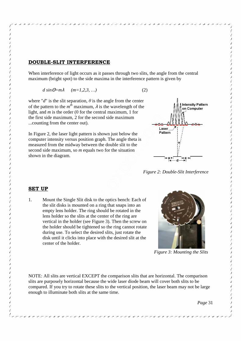
DOUBLE-SLIT INTERFERENCE When interference of light occurs as it passes through two slits, the angle from the central maximum (bright spot) to the side maxima in the interference pattern is given by d sinΘ=mλ (m=1,2,3, …) (2) where "d" is the slit separation, θ is the angle from the center of the pattern to the mth maximum, λ is the wavelength of the light, and m is the order (0 for the central maximum, 1 for the first side maximum, 2 for the second side maximum ...counting from the center out). In Figure 2, the laser light pattern is shown just below the computer intensity versus position graph. The angle theta is measured from the midway between the double slit to the second side maximum, so m equals two for the situation shown in the diagram. Figure 2: Double-Slit Interference SET UP 1. Mount the Single Slit disk to the optics bench: Each of
the slit disks is mounted on a ring that snaps into an empty lens holder. The ring should be rotated in the lens holder so the slits at the center of the ring are vertical in the holder (see Figure 3). Then the screw on the holder should be tightened so the ring cannot rotate during use. To select the desired slits, just rotate the disk until it clicks into place with the desired slit at the center of the holder.
NOTE: All slits are vertical EXCEPT the comparison slits that are horizontal. The comparison slits are purposely horizontal because the wide laser diode beam will cover both slits to be compared. If you try to rotate these slits to the vertical position, the laser beam may not be large enough to illuminate both slits at the same time.
Figure 3: Mounting the Slits
Page 32
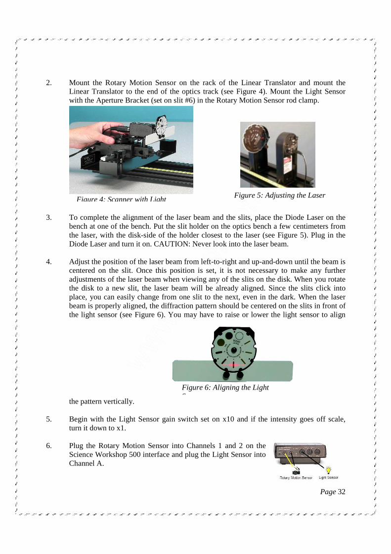
2. Mount the Rotary Motion Sensor on the rack of the Linear Translator and mount the
Linear Translator to the end of the optics track (see Figure 4). Mount the Light Sensor with the Aperture Bracket (set on slit #6) in the Rotary Motion Sensor rod clamp.
3. To complete the alignment of the laser beam and the slits, place the Diode Laser on the
bench at one of the bench. Put the slit holder on the optics bench a few centimeters from the laser, with the disk-side of the holder closest to the laser (see Figure 5). Plug in the Diode Laser and turn it on. CAUTION: Never look into the laser beam.
4. Adjust the position of the laser beam from left-to-right and up-and-down until the beam is
centered on the slit. Once this position is set, it is not necessary to make any further adjustments of the laser beam when viewing any of the slits on the disk. When you rotate the disk to a new slit, the laser beam will be already aligned. Since the slits click into place, you can easily change from one slit to the next, even in the dark. When the laser beam is properly aligned, the diffraction pattern should be centered on the slits in front of the light sensor (see Figure 6). You may have to raise or lower the light sensor to align
the pattern vertically. 5. Begin with the Light Sensor gain switch set on x10 and if the intensity goes off scale,
turn it down to x1. 6. Plug the Rotary Motion Sensor into Channels 1 and 2 on the
Science Workshop 500 interface and plug the Light Sensor into Channel A.
Figure 6: Aligning the Light Sensor
Figure 5: Adjusting the Laser Figure 4: Scanner with Light
Page 33
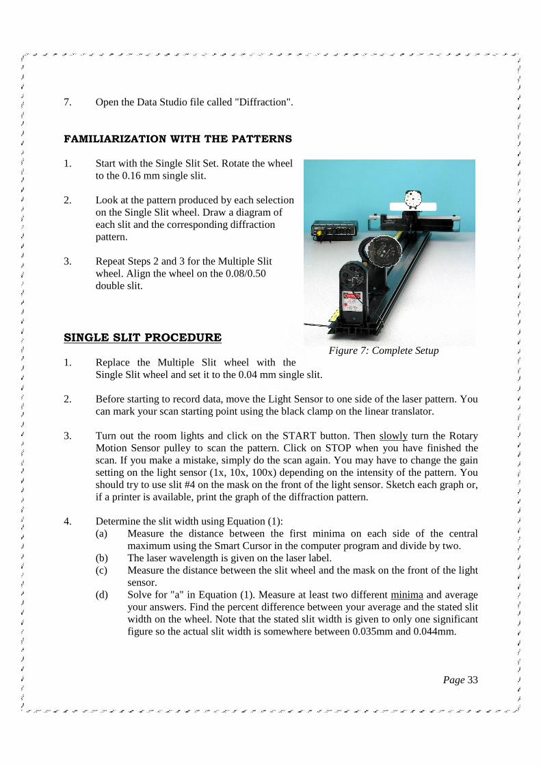
7. Open the Data Studio file called "Diffraction". FAMILIARIZATION WITH THE PATTERNS
1. Start with the Single Slit Set. Rotate the wheel
to the 0.16 mm single slit. 2. Look at the pattern produced by each selection
on the Single Slit wheel. Draw a diagram of each slit and the corresponding diffraction pattern.
3. Repeat Steps 2 and 3 for the Multiple Slit
wheel. Align the wheel on the 0.08/0.50 double slit.
SINGLE SLIT PROCEDURE 1. Replace the Multiple Slit wheel with the
Single Slit wheel and set it to the 0.04 mm single slit. 2. Before starting to record data, move the Light Sensor to one side of the laser pattern. You
can mark your scan starting point using the black clamp on the linear translator. 3. Turn out the room lights and click on the START button. Then slowly turn the Rotary
Motion Sensor pulley to scan the pattern. Click on STOP when you have finished the scan. If you make a mistake, simply do the scan again. You may have to change the gain setting on the light sensor (1x, 10x, 100x) depending on the intensity of the pattern. You should try to use slit #4 on the mask on the front of the light sensor. Sketch each graph or, if a printer is available, print the graph of the diffraction pattern.
4. Determine the slit width using Equation (1): (a) Measure the distance between the first minima on each side of the central
maximum using the Smart Cursor in the computer program and divide by two. (b) The laser wavelength is given on the laser label. (c) Measure the distance between the slit wheel and the mask on the front of the light
sensor. (d) Solve for "a" in Equation (1). Measure at least two different minima and average
your answers. Find the percent difference between your average and the stated slit width on the wheel. Note that the stated slit width is given to only one significant figure so the actual slit width is somewhere between 0.035mm and 0.044mm.
Figure 7: Complete Setup

Page 34
DOUBLE SLIT PROCEDURE 1. Replace the single slit disk with the multiple slit disk.
Set the multiple slit disk on the double slit with slit separation 0.25 mm (d) and slit width 0.04 mm (a).
2. Set the Light Sensor Aperture Bracket to slit #4. 3. Before starting to record data, move the Light Sensor to
one side of the laser pattern, up against the linear translator stop. 4. Turn out the room lights and click the START button. Then slowly turn the Rotary
Motion Sensor pulley to scan the pattern. Click STOP when you have finished the scan. You may have to change the gain setting on the light sensor (1x, 10x, 100x) depending on the intensity of the pattern. To get the most detail, use the smallest slit possible on the Light Sensor mask.
5. Use the magnifier to enlarge the central maximum and the first side maxima. Use the
Smart tool to measure the distance between the central maximum and the first side maxima.
6. Measure the distance between the central maximum and the second and third side
maxima. Also measure the distance from the central maximum to the first minimum in the DIFFRACTION (not interference) pattern.
7. Determine the slit separation using Equation (2): (a) Measure the distance between the slit wheel and the mask on the front of the light
sensor. (b) Solve for "d" in Equation (2). Determine "d" using the first, second, and third
maxima and find the average "d". Find the percent difference between your average and the stated slit separation on the wheel.
8. Determine the slit width using Equation (1) and the distance between the central
maximum and the first minimum in the diffraction pattern (not interference pattern). Is this the slit width given on the wheel?
9. Repeat Steps 2 through 8 for the interference patterns for the double slits (a/d = 0.04/0.50
mm).
Page 35
OBSERVATION: Make the observation table in position and Light intensity for single slit.
S.No. Position (in cm) Light Intensity (% max)
Make the observation table in position and Light intensity for Double slit.
S.No. Position (in cm) Light Intensity (% max)
DATA PROCESSING: Plot a Graph between position (horizontal axis) and Light Intensity (vertical axis) for Single slit. And Plot a Graph between position (horizontal axis) and Light Intensity (vertical axis) for Double slit. QUESTIONS 1. What physical quantity is the same for the single slit and the double slit? 2. How does the distance from the central maximum to the first minimum in the single-slit
pattern compare to the distance from the central maximum to the first diffraction minimum in the double-slit pattern?
3. What physical quantity determines where the amplitude of the interference peaks goes to zero?
4. In theory, how many interference maxima should be in the central envelope for a double slit with d = 0.25 mm and a = 0.04 mm?

Page 36
EXPERIMENT 6:
INTERFERENCEINTERFERENCEINTERFERENCEINTERFERENCE BY FRESNEL’S BIPRISMBY FRESNEL’S BIPRISMBY FRESNEL’S BIPRISMBY FRESNEL’S BIPRISM
AIMS/OBJECT: To Study the interference by Fresnel’s biprism and find out the fringe width β. APPARATUS USED: 1 Basic Optics Track, 1.2 m 2 Basic Optics Slit 3 Basic Optics Diode Laser 4 Bi-Prism 5 Aperture Bracket 6 Linear Translator 7 Light Sensor 8 Rotary Motion Sensor 9 Science Workshop 500 or 750 Interface 10 Data Studio 11. Computer set.
INTRODUCTION: While the results of Young’s double slit experiment quite clearly indicate interference and the wave nature of light, when the experiment was first done objections were raised that the results were not conclusive since there could have been diffraction effects from the edge of the slits. To counter this, Augustine Fresnel proposed a series of interference experiments that would have no diffracting edges. The most notable of these is the Fresnel Biprism, where two virtual sources are created by refraction through a biprism. The interference of two coherent light sources occurs when waves of equal amplitude of meet. They produce an interference pattern, consisting of a succession of bright and dark fringes called intensity minima and maxima. PRINCIPLE: The Fresnel biprism is a prism which has one of its angles slightly less than two right angles and two equal small base angles. It acts like two very thin prisms placed base to base. When rays from a slit, , illuminated by a monochromatic light, such as sodium light are made to be incident on the plane face of the biprism (PQR), the emergent rays from the two halves of the biprism appear to diverge from two coherent virtual sources, S1 and S2. If a screen (AB) is placed with its plane perpendicular to the plane containing the slit and the common base of the biprism, the emergent beams of light overlap on the screen producing alternate dark and bright fringes.

Page 37
If d is the distance between the two virtual sources S1 and S2, D is the distance between the slit and the screen, and λ is the wavelength of the monochromatic radiation, then the fringe width, β, i.e., the distance between two consecutive dark or bright fringes is given by β = λ D / d.
FORMULA USED: The wavelength of monochromatic light is given by the formula in the case of Bi-prism experiment.
λ = β . (d / D)

Page 38
Where λ = Wavelength of given source (650 nm) β = Fringe width d = distance between two virtual sources D = distance between slit and screen PROCEDURE 1. Mount the gadgets on the optical bench.
2. Study all the movements on each stand.
3. Ensure that all the pieces are aligned at roughly the same height
4. Adjust the slit width to get the best compromise between brightness and sharpness of the fringe
pattern.
5. Open data studio software and click for interference & diff. Make a graph between position and
light intensity
6. Without disturbing the positions of the slit, biprism and the screen sense the pattern in form of
graph between position and light intensity.
7. Measure the distance d between two virtual sources.
8. Measure the fringe width or distance between two consecutive dark or bright fringes.
9. Using formula calculate wavelength and fringe width β.

Page 39
OBSERVATION:
Make the observation table in position and Light intensity.
S.No. Position (in cm) Light Intensity I (% max)
DATA PROCESSING: Plot a Graph between position (horizontal axis) and Light Intensity (vertical axis). And get the distance (d) between two virtual sources. CALCULATION: λ = β . (d / D) RESULTS: The fringe width β = …………mm CONCLUSION: Thus this experiment demonstrates how the Fresnel Biprism can be used to demonstrate Fringes obtained due to interference and can be used to calculate the fringe width and also the refractive index of a thin transparent plastic sheet. Adjustments must be made carefully before proceeding with the experiment to avoid errors.

Page 40
EXPERIMENT 7:
CAUCHY’S CONSTANT USING PRISMCAUCHY’S CONSTANT USING PRISMCAUCHY’S CONSTANT USING PRISMCAUCHY’S CONSTANT USING PRISM
AIMS/OBJECT: 1. To determine the refractive indices of a glass prism at various wavelength of mercury light. 2. To plot the dispersion curve for the given glass prism and calculate the Dispersive power of the prism. 3. To obtain the coefficient in Cauchy’s equation from the graph of n vs (1/λ2). APPARATUS:
1 Prism spectrometer 2 Prism 3 Prism clamp 4 Reading lens 5 Spectral lamp with spectral power supply
PRINCIPLE: The most general form of Cauchy's equation is n = A + B / λ2 + C/ λ4 +……………
where n is the refractive index, λ is the wavelength, A, B, C, etc., are coefficients that can be determined for a material by fitting the equation to measured refractive indices at known wavelengths. The coefficients are usually quoted for λ as the vacuum wavelength in micrometers. Usually, it is sufficient to use a two-term form of the equation:
n = A + B / λ2
Where the coefficients A and B are determined specifically for this form of the equation.
This is known as Cauchy’s equation, the constant A is called the coefficient of refraction and B is known as the coefficient of dispersion. Note that the coefficient of refraction is different from the index of refraction. Cauchy’s equation is an approximation and applies reasonably well to many non-absorbing materials, in the optical region. When a parallel beam goes through the prism getting refracted twice, the emergent beam bends through some angle with respect to the incident beam. This angle is called the angle of deviation. It changes with the angle of incidence and is minimum when the incident and emergent beams make equal angles with the corresponding refracting surfaces.
Apex angle A
D Angle of minimum deviation

Page 41
The angle of minimum deviation D is related to the angle of prism A and the refractive index n of the material of the prism as A narrow beam of light from a spectral line source, which emits visible radiation of characteristic and known wavelengths, is made incident on the prism. By measuring the minimum deviation corresponding to each wavelength we may establish the dependence of n upon λ. The dispersive power of a material is defined by the equation ω = (nB –nR) / (nY- 1) Where nB , nR and nY are refractive endices of material for blue, red, and yellow lights respectively. The reciprocal of the dispersive power is called dispersive index and it lies between 20 and 60 for most optical glasses.
PROCEDURE:
� Adjustment of the spectrometer:
• Locate which is collimator and which is telescope. The one next to the lamp is collimator. Adjust the spectrometer if needed. Take care not to play with any knob or screw without reason. The spectrometer is reasonably adjusted and you may only have to perform the checks to ensure it. Check the following. Look at the slit through the collimator. It should be clear sharp, rectangular in shape. You can increase or decrease the slit width to get this. It should be narrow but the whole rectangular area should be well illuminated.
Now bring the telescope in line with the collimator and look at the slit through the telescope. It should be a sharp image at the centre of the field of view.
• Level the prism table using a sprit level and three screws provided on the table if
necessary.
• See how the prism table can be rotated of locked. Also see how the telescope can be rotated and the angle can be measured using vernier scale given.
Sin {(A+D) / 2} n = Sin (A/2)

Page 42
� The measurement of the refracting angle A of the prism
• Place the prism on its triangular base so that its refracting edge is at the center of the prism table and points towards the collimator.
• Turn the prism table such that about half of the light falls on each refracting face. Lock the prism table. You should be able to see the image of the slit with naked eye on reflection from either face of the prism.
• Now rotate the telescope to receive the reflected light on one side of the prism. Do the same on the other side. If the instrument is correctly leveled the images from both sides fall at the center of the telescope cross wire. If necessary, adjust the entrance slit width of the collimator to sharpen the image.
• Bring one edge of the slit image into coincidence with the intersection of the crosswire and lock the telescope. Record the reading using the vernier. Do the same on the other side. Use the same vernier each time.
From these measurements, calculate the refracting angle A of the prism. � Angle of minimum deviation and its measurement: • Put the prism on the prism table such that the center of the base of the prism is at the
center of the prism table. Rotate the prism table so that the beam from the collimator falls on one of the refracting surfaces and emerges through the other. The spectral lines should be visible with the unaided eye. Locate the spectrum with the telescope. On emergence you will see slit images of different colours at different angles. The whole thing is called a spectrum. Select a particular line in the spectrum for observation and note its colour and the corresponding wavelength in your observation table. Lock the platform. If necessary, adjust the entrance slit width of the collimator to sharpen the spectrum so that it is as bright as possible. Now rotate the prism table slowly in steps and each time rotate the telescope to receive the selected line at the cross wire. The telescope should come closer to the direct path. If it goes away from the direct path, rotate the prism table in opposite direction. You cannot bring the line closer to the direct path beyond a point. As you rotate the prism table in either direction at this stage, the image will move away from the direct path. This turning point is the position of minimum deviation for that particular wavelength.
S Collimator Telescope Prism 2A Measurement of Prism angle

Page 43
If you lock the telescope in this position, disturb the prism table a little bit, and gradually rotate it to bring it back to the original position and continue in the same sense, the successive view that you will see in the telescope are like that shown in fig.
Slit image image just
reaches centre image recedes cross wire 1 2 3 4 5
• Determine this position very carefully by using the fine adjustment screws on the
telescope. Record the reading at the vernier. Res determine this position for the same line several times and take the average minimum deviation position Dj.
• Repeat the same procedure for all the spectral lines that can be seen clearly record all observations carefully.
• Remove the prism and rotate the telescope to bring it directly opposite to the collimator in a straight line. Center the slit image in the cross wire and record this position using the vernier. You may take several readings to get an average value of this zero point position. Do the angle of minimum deviation (D) for the jth spectral line ׀Dj-D0׀.
OBSERVATION: Table for the angle (A) of the Prism.
S. No.
Vernier
Telescope reading for reflection from first face
Telescope reading for reflection from first face
Difference a-b =2A
Mean value of 2A
A
Mean A degrees M.S V.S Total
(a) M.S V.S Total
(b) 1 V1
V2
2 V1
V2

Page 44
Table for the angle of Minimum deviation the Prism. S. No.
Colour
Vernier
Dispersed image Telescope in minimum deviation position
Telescope reading for Direct image
Difference a – b
Mean δm deviation (Degree) M.S V.S Total
(a) M.S V.S Total
(b) 1 Violet V1
V2 2 Blue V1
V2 3 Green V1
V2 4 Yellow V1
V2 5 Red V1
V2 Colour Wavelength
λ (in µm) 1 / λ2
Angle of Deviation
Index of Refraction (n)
Red 0.6273 Yellow 0.5798 Green 0.5477 Blue 0.4385 Violet 0.4051 CALCULATION: Make necessary calculations for the refractive index n. DATA PROCESSING: Plot graph between n vs 1/λ2. Find a best straight line fit to the graph. Calculate the slope and the y-intercept QUESTIONS:
1. On what factor does the angle of deviation depend when a beam of light passes through a prism?
2. Why is it necessary to make the beam parallel by passing through the collimator?
Page 45
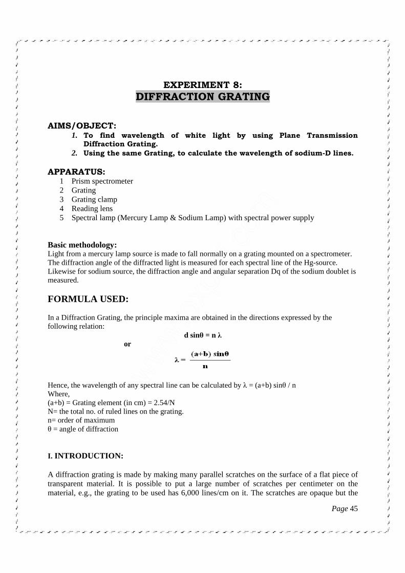
EXPERIMENT 8:
DIFFRACTION GRATING
AIMS/OBJECT:
1. To find wavelength of white light by using Plane Transmission Diffraction Grating.
2. Using the same Grating, to calculate the wavelength of sodium-D lines. APPARATUS:
1 Prism spectrometer 2 Grating 3 Grating clamp 4 Reading lens 5 Spectral lamp (Mercury Lamp & Sodium Lamp) with spectral power supply
Basic methodology: Light from a mercury lamp source is made to fall normally on a grating mounted on a spectrometer. The diffraction angle of the diffracted light is measured for each spectral line of the Hg-source. Likewise for sodium source, the diffraction angle and angular separation Dq of the sodium doublet is measured.
FORMULA USED: In a Diffraction Grating, the principle maxima are obtained in the directions expressed by the following relation:
d sinθ = n λ or
Hence, the wavelength of any spectral line can be calculated by λ = (a+b) sinθ / n Where, (a+b) = Grating element (in cm) = 2.54/N N= the total no. of ruled lines on the grating. n= order of maximum θ = angle of diffraction I. INTRODUCTION: A diffraction grating is made by making many parallel scratches on the surface of a flat piece of transparent material. It is possible to put a large number of scratches per centimeter on the material, e.g., the grating to be used has 6,000 lines/cm on it. The scratches are opaque but the

Page 46
areas between the scratches can transmit light. Thus, a diffraction grating becomes a multitude of parallel slit sources when light falls upon it.
A parallel bundle of rays falls on the grating. Rays and wave fronts form an orthogonal set so the wave fronts are perpendicular to the rays and parallel to the grating as shown. Utilizing Huygens' Principle, which is that every point on a wavefront acts like a new source, each transparent slit becomes a new source so cylindrical wave fronts spread out from each. These wave fronts interfere either constructively or destructively depending on how the peaks and valleys of the waves are related. If a peak falls on a valley consistently (called destructive interference), then the waves cancel and no light exists at that point. On the other hand, if peaks fall on peaks and valleys fall on valleys consistently (called constructive interference), then the light is made brighter at that point.
Consider two rays which emerge making an angle with the straight through line. Constructive interference (brightness) will occur if the difference in their two path lengths is an integral multiple of their wavelength () i.e., difference = n where n = 1, 2, 3, ... Now, a triangle is formed, as indicated in the diagram, for which
n = d sin( ) and this is known as the DIFFRACTION GRATING EQUATION . In this formula is the angle of emergence (called deviation, D, for the prism) at which a wavelength will be bright, d is the distance between slits (note that d = 1 / N if N, called the grating constant, is the number of lines per unit length) and n is the "order number", a positive integer (n = 1, 2, 3, ...) representing the repetition of the spectrum.
Thus, the colors present in the light from the source incident on the grating would emerge each at a different angle since each has a different wavelength . Furthermore, a complete spectrum would be observed for n = 1 and another complete spectrum for n = 2, etc., but at larger angles.

Page 47
Also, the triangle formed by rays to the left of 0o is identical to the triangle formed by rays to the right of 0o but the angles R and L (Right and Left) would be the same only if the grating is perpendicular to the incident beam. This perpendicularity is inconvenient to achieve so, in practice, R and L are both measured and their average is used as in the grating equation.
Sodium D lines The sodium doublet is responsible for the bright yellow light from a sodium lamp. The doublet arises from the 3p®3s transition, in the sodium atom. The 3p level splits into two closely spaced level with an energy spacing of 0.0021 eV.
The splitting occurs due to the spin orbit effect. This can be crudely thought of as arising due to the Internal magnetic field produced by the electron’s circulation around the nucleus and the splitting takes place anologus to the Zeeman Effect. Fig. 4 shows the 3p and 3s levels their splitting and the radiative transition that produces the sodium doublets or D lines.
PROCEDURE
Measuring
1. CAUTION: The diffraction grating is a photographic reproduction and should NOT be touched. The deeper recess in the holder is intended to protect it from damage. Therefore, the glass is on the shallow side of the holder and the grating is on the deep side.
2. Place the grating on the center of the table with its scratches running vertically, and with the base material (glass) facing the light source.
3. Rotate the table to make the grating perpendicular to the incident beam by eye. This is not critical since the average of R and L accommodates a minor misalignment.

Page 48
4. Affirm maximum brightness for the straight through beam by adjusting the source-slit alignment. At this step, the slit should be narrow, perhaps a few times wider than the hairline. Search for the spectrum by moving the telescope to one side or the other. This spectrum should look much like that observed with the prism except that the order of the colors as you move away from zero degrees is reversed.
5. Search for the second- and third-order spectra. Do not measure the higher-order angles, but record the order of colors away from zero degrees.
6. For each of the seven colors in the mercury spectrum, measure the angles R and L to the nearest tenth of a degree by placing the hairline on the stationary side of the slit.
PART B: To measure the wavelength of second sodium light (D2) In first order spectrum of sodium measure the angular position qL of yellow 1 (D1) on the left side. Use the micrometer screw to turn the telescope to align the crosswire at the second yellow line (D2) and read its angular position qL. Likewise measure qR on the RHS for D1 and D2. Method to make light fall normal to the grating surface: a) First mount grating approximately normal to the collimator. See the slit through telescope and take reading from one side of vernier window. Note down the reading. b) Add or subtract (whichever is convenient) 900 from reading taken in step (a) and put telescope to this position. In this position telescope is approximately perpendicular to the collimator. c) Now rotate prism table until the slit is visible on the cross-wire of the telescope. At this position the incident light from the collimator falls at an angle 450 with the plane of the grating. Note down this reading. d) Next add or subtract 45o to step (c) reading and rotate the prism table so as to obtain this reading on the same window. In this situation, light incident in the grating surface is perpendicular.

Page 49
OBSERVATION: No. of ruling per inch on grating = ……….. Least count of spectrometer = …………. Reading of Telescope for direct image =………. Reading of telescope after rotating it through 900 = ……. Reading of circular scale when reflected image is obtained on cross wire = …… Reading after the rotating prism table through 450 or 1350 = Table for the angle of Diffraction. Order of Spectrum
Colour
Vernier
Spectrum on Left side Reading of Telescope
Spectrum on Right side Reading of Telescope
Difference 2θ= a – b
Mean (Degree) M.S V.S Total
(a) M.S V.S Total
(b) 1
Violet V1 V2
Blue V1 V2
Green V1 V2
Yellow V1 V2
Red V1 V2
2
Violet V1 V2 Blue V1 V2 Green V1 V2 Yellow V1 V2 Red V1 V2
CALCULATION : The wavelength of spectral lines is calculated by
(A) For I order spectrum:
(B) For II order spectrum:
RESULT: The wavelength of spectral lines are …………..in nm (all colour for I order) The wavelength of spectral lines are …………..in nm (all colour for II order)

Page 50
ERROR ANALYSIS:
For all colour PRECAUTIONS: 1. The experiment should be performed in a dark room. 2. Micrometer screw should be used for fine adjustment of the telescope. For fine adjustment the telescope should be first licked by means of the head screw. 3. The directions of rotation of the micrometer screw should be maintained otherwise the play in the micrometer spindle might lead to errors. 4. The spectral lams (mercury source) attain their full illuminating power after being warmed up for about 5 minutes; observation should be taken after 5 minutes. 5. One of the essential precautions for the success of this experiment is to set the grating normal to the incident rays (see below). Small variation on the angle of incident causes correspondingly large error in the angle of diffraction. If the exact normally is not observed, one find that the angle of diffraction measured on the left and on the right are not exactly equal. Read both the verniers to eliminate any errors due to no coincidence of the center of the circular sale with the axis of rotation of the telescope or table.

Page 51
EXPERIMENT 9:
POLARIZATIONPOLARIZATIONPOLARIZATIONPOLARIZATION
AIM / OBJECT: To study the Polarization of light (Malus’s Law). Malus law of polarization is verified by showing that the intensity of light passed through two polarizers depends on the square of the cosine of the angle between the two polarization axes. APPRATUS USED:
1 Polarization Analyzer 2 Basic Optics Bench (60 cm) 3 Aperture Bracket 4 Red Diode Laser 5 Light Sensor 6 Rotary Motion Sensor 7 Science Workshop 500 Interface 8 Data Studio Software
INTRODUCTION Laser light (peak wavelength = 650 nm) is passed through two polarizers. As the second polarizer (the analyzer) is rotated by hand, the relative light intensity is recorded as a function of the angle between the axes of polarization of the two polarizers. The angle is obtained using a Rotary Motion Sensor that is coupled to the polarizer with a drive belt. The plot of light intensity versus angle can be fitted to the square of the cosine of the angle. THEORY A polarizer only allows light which is vibrating in a particular plane to pass through it. This plane forms the "axis" of polarization. Unpolarized light vibrates in all planes perpendicular to the direction of propagation. If unpolarized light is incident upon an "ideal" polarizer, only half of the light intensity will be transmitted through the polarizer.
Figure 1: Light Transmitted through Two Polarizers

Page 52
The transmitted light is polarized in one plane. If this polarized light is incident upon a second polarizer, the axis of which is oriented such that it is perpendicular to the plane of polarization of the incident light, no light will be transmitted through the second polarizer. See Fig.1. However, if the second polarizer is oriented at an angle not perpendicular to the axis of the first polarizer, there will be some component of the electric field of the polarized light that lies in the same direction as the axis of the second polarizer, and thus some light will be transmitted through the second polarizer.
U n po lari zed E -f i e ld
E o ����
E E����
P o lar ize r #1 P o lar ize r #2
Figure 2: Component of the Electric Field
If the polarized electric field is called E0 after it passes through the first polarizer, the component, E, after the field passes through the second polarizer which is at an angle φ with respect to the first polarizer is E0cosφ (see Fig.2). Since the intensity of the light varies as the square of the electric field, the light intensity transmitted through the second filter is given by
φ2cosoII = (1)
SET UP
Figure 3: Equipment Components Figure 4: Interface with Sensors
Page 53
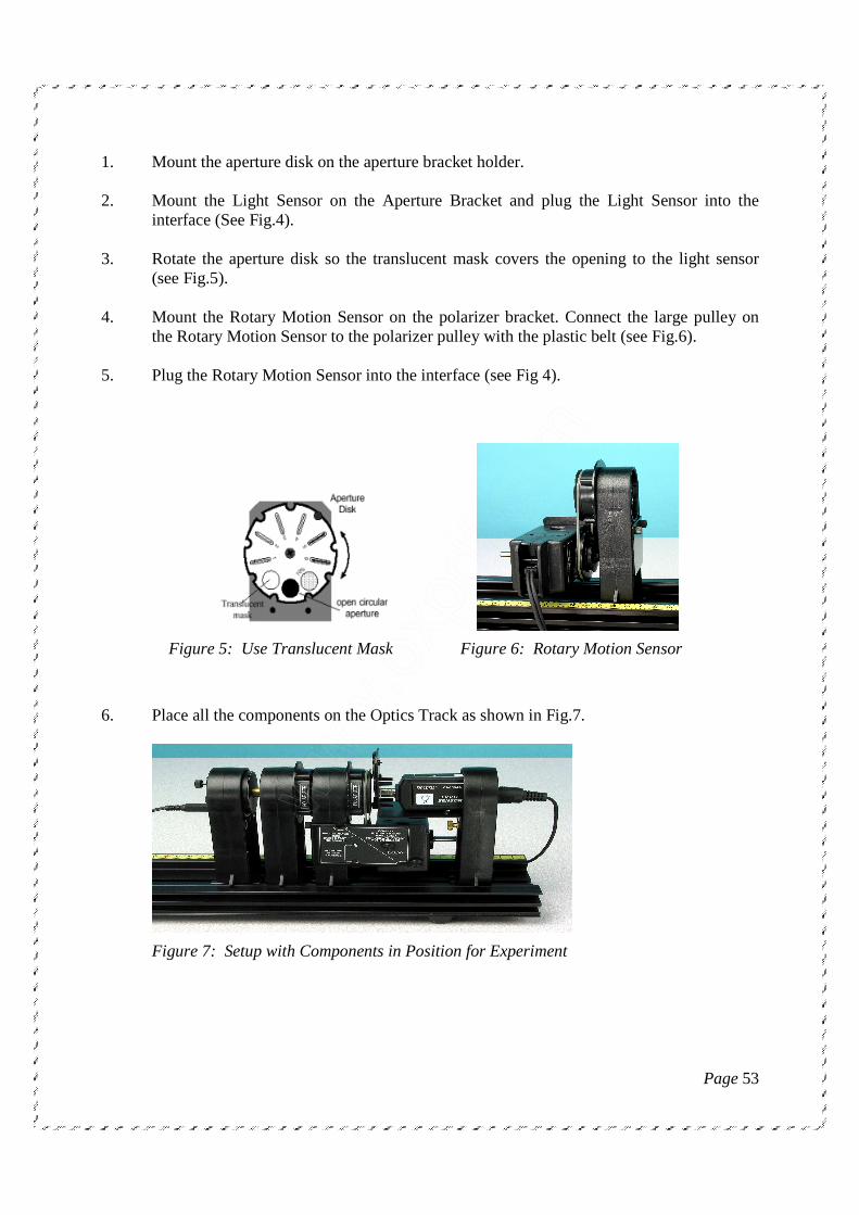
1. Mount the aperture disk on the aperture bracket holder. 2. Mount the Light Sensor on the Aperture Bracket and plug the Light Sensor into the
interface (See Fig.4). 3. Rotate the aperture disk so the translucent mask covers the opening to the light sensor
(see Fig.5). 4. Mount the Rotary Motion Sensor on the polarizer bracket. Connect the large pulley on
the Rotary Motion Sensor to the polarizer pulley with the plastic belt (see Fig.6). 5. Plug the Rotary Motion Sensor into the interface (see Fig 4).
Figure 5: Use Translucent Mask Figure 6: Rotary Motion Sensor
6. Place all the components on the Optics Track as shown in Fig.7.
Figure 7: Setup with Components in Position for Experiment

Page 54
PROCEDURE FOR 2 POLARIZERS In the first two procedure steps, the polarizers are aligned to allow the maximum amount of light through. 1. Since the laser light is already polarized, the first polarizer must be aligned with the
laser's axis of polarization. First remove the holder with the polarizer and Rotary Motion Sensor from the track. Slide all the components on the track close together and dim the room lights. Click START and then rotate the polarizer that does not have the Rotary Motion Sensor until the light intensity on the graph is at its maximum. You may have to use the button in the upper left on the graph to expand the graph scale while taking data to see the detail.
2. To allow the maximum intensity of light through both polarizers, replace the holder with
the polarizer and Rotary Motion Sensor on the track, press Start, and then rotate polarizer that does have the Rotary Motion Sensor until the light intensity on the graph is at its maximum (see Fig. 8).
Figure8: Rotate the Polarizer That Has the Rotary Motion Sensor
3. If the maximum exceeds 4.5 V, decrease the gain on the switch on the light sensor. If the
maximum is less than 0.5 V, increase the gain on the switch on the light sensor. 4. Press Start and slowly rotate the polarizer which has the Rotary Motion Sensor through
180 degrees. Then press Stop.

Page 55
OBSERVATION:
Make the observation table in Angular position and Light intensity.
S.No. Angular Position θ (in Degree) Light Intensity I (% max)
DATA PROCESSING: Plot a Graph between Angular position (horizontal axis) and Light Intensity (vertical axis). CALCULATION: Make necessary calculations for verify the Malus’s Law. ANALYSIS 1. Click on the Fit button on the graph. Choose the User-Defined Fit and write an equation
(Acos(x)^2) with constants you can adjust to make the curve fit your data. 2. Try a cos3(φ) fit and then try a cos4(φ) fit. Does either of these fit better than your
original fit? Does the equation that best fits your data match theory? If not, why not?

Page 56
EXPERIMENT 10:
ELECTRON DIFFRACTIONELECTRON DIFFRACTIONELECTRON DIFFRACTIONELECTRON DIFFRACTION
AIM/ OBJECT: To study the Electron diffraction and verify the de-Broglie equation. APPARATUS USED:
1. High voltage Power Supply (U33010-230)
2. Tube Holder S (U185001)
3. Connecting cords
THEORY The electron diffraction tube illustrates the wave nature of electrons by allowing observation of interference caused by a beam of electrons passing through a polycrystalline graphite target on a fluorescent screen (Debye-Scherer diffraction). The wavelength of electrons can be calculated for various anode voltages from the radius of the diffracted rings and the distance between the crystal layers in the graphite. The tube also confirms the de-Broglie hypothesis. The electron diffraction tube is highly evacuated tube with an electron gun consisting of a pure tungsten heater filament (4) and a cylindrical anode (5) all contained in a clear glass bulb. The electrons emitted by the heated cathode are constrained to a narrow beam by an aperture and are then focused by means of an electron optical system. The resulting tight, monochromatic beam then passes through a micro mesh nickel grating situated at the aperture of the gun. Onto this grid, a thin layer of polycrystalline graphitized carbon has been deposited by vaporization. This layer affects the electrons in the beam much like a diffraction grating. The result of this diffraction is seen in the form of an image comprising two concentric rings that become visible
1 2 3 4 5 6 7 8 Electron Diffraction Tube S U18571
1 Guide pin
2 Connection pin
3 Cathode
4 Heater Filament
5 Anode
6 Focusing electrode
7 Polycrystalline
graphite grating
8 Fluorescent screen

Page 57
on the fluorescent screen. A spot resulting from the undeflected electron beam continues to be visible at the centre of the rings. A magnet is also supplied with the tube. This allows the direction of the electron beam to be changed, which may be necessary if the graphite target has slight damage as a result of the manufacturing process due to later overheating.
TECHNICAL DATA Filament voltage: ≤ 7.5 V AC/DC Anode voltage: 0- 5000V DC Anode current: typ. 0.15mA bei 4000V DC Lattice constant of graphite: d10 = 0.213 nm d11 = 0.123 nm Dimensions: Distance from graphite target To fluorescent screen: 135 mm approx. Fluorescent screen: 100 mm dia. approx. Glass bulb: 130 mm dia approx. Total length: 260 mm dia. approx. OPERATION
1. Setting up the electron diffraction tube in the tube holder. Press tube gently into the stock of the holder and push until the pins are fully inserted. Take note of the unique position of the guide pin.
2. Removing the electron diffraction tube from the tube holder. To remove the tube, apply pressure with the middle finger on the guide pin and the thumb on the tail stock until the pins loosen, then pull out the tube.
GENERAL INSTRUCTIONS The graphite foil on the diffraction grating is only a few layers of molecules thick and any current greater 0.2 mA can cause its destruction. The anode voltage and the graphite target itself should be monitored throughout the experiment. If the graphite target starts to glow or the emission current rises above 0.2 mA, the anode must immediately be disconnected from its power supply. If the diffraction rings are not satisfactorily visible, the electron beam can be redirection by a magnet so that it passes through an undamaged region of the target.

Page 58
EXPERIMENT INSTRUCTIONS
• Set the experiment as in fig 2. • Apply the heater voltage and wait about one minute for the heater temperature to achieve
thermal stability. • Apply an anode voltage of 4 KV. • Determine the diameter D of the diffraction rings.
• Two diffraction rings appear on the fluorescent screen centered on the undeflected beam
in the middle. The two rings correspond to Bragg reflections from atoms in the layers of the graphite crystal lattice.
• Changing the anode voltage causes the rings to change in diameter. Reducing the voltage
makes the rings wider. This supports de-Broglie’s postulate that the wavelength increases as momentum is reduced.
From Bragg’s equation: λ = 2.d.SinӨ Tan 2Ө = D/ 2L Where: λ = wave length of the electrons Ө = glancing angle of the diffraction ring d = lattice plane spacing in graphite L = distance between sample and screen D = diameter D of the diffraction ring R = radius of the diffraction ring
From De-Broglie’s equation: λ = h / p e.V = p2 / 2.m
Where: h = Plank’s constant p = momentum of electron m = mass of electron e = electron charge V= applied voltage
λ = d. R /L
λ = h /√ 2.m.e.V
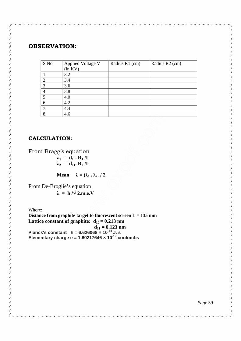
Page 59
OBSERVATION:
S.No. Applied Voltage V
(in KV) Radius R1 (cm) Radius R2 (cm)
1. 3.2 2. 3.4 3. 3.6 4. 3.8 5. 4.0 6. 4.2 7. 4.4 8. 4.6
CALCULATION: From Bragg’s equation
λ1 = d10. R1 /L λ2 = d11. R2 /L Mean λ = (λ1 + λ2) / 2
From De-Broglie’s equation
λ = h /√ 2.m.e.V
Where: Distance from graphite target to fluorescent screen L = 135 mm Lattice constant of graphite: d10 = 0.213 nm d11 = 0.123 nm Planck's constant h = 6.626068 × 10 -34 J. s Elementary charge e = 1.60217646 × 10 -19 coulombs

Page 60
2Ө D L
Fig:1 Schematic representation to Debye Scherrer diffraction
UA UF Fig:2 Circuit diagram for the diffraction tube
F3 F4 C5 G7
U33010 _ +
I

Page 61
EXPERIMENT 11:
PHOTOELECTRIC EFFECTPHOTOELECTRIC EFFECTPHOTOELECTRIC EFFECTPHOTOELECTRIC EFFECT
AIM / OBJECT:
Measuring and Calculating Plank's Constant (h). Plot a graph of Stopping Potential versus frequency and use a linear best fit curve to determine the slope. The slope is the ratio of h/e so Planck's constant (h) is found by multiplying this value by the charge of an electron (e =1.602 x 10⁻¹⁹ C) APPRATUS USED:
1. Photoelectric Effect Apparatus 2. Optical Filters Box 3. Mercury Light Source Enclosure 4. Base 5. Photodiode Enclosure 6. Power Supply
INTRODUCTION: The photoelectric effect is the emission of electrons from the surface of a metal when electromagnetic radiation (such as visible or ultraviolet light) of the right frequency shines on the metal. At the time of its discovery, the classical wave model for light predicted that the energy of the emitted electrons would increase as the intensity (brightness) of the light increased. Instead it was discovered that the energy of the emitted electrons was directly proportional to the frequency of the incident light, and that no electrons would be emitted if the light source was not above a certain threshold frequency. Lower energy electrons were emitted when light with relatively low frequency was incident on the metal, and higher energy electrons were emitted when light with relatively high frequency was incident on the metal. The AP-8209 Photoelectric Effect Apparatus consists of a mercury light source enclosure, a photodiode tube enclosure, a base, the photoelectric effect test instrument, miscellaneous cords and cables, a power supply for the mercury light source and the test instrument, and a box of apertures, filters, caps, and alignment screws. The apparatus has several important features:
• The current amplifier has high sensitivity and is very stable in order to improve the accuracy of the measurement.
• The photoelectric tube has low levels of dark current and anode reverse current. • The optical filters are of high quality in order to avoid an error due to interference
between different spectral lines.
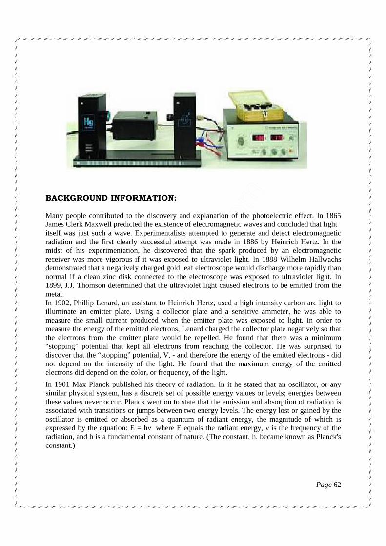
Page 62
BACKGROUND INFORMATION: Many people contributed to the discovery and explanation of the photoelectric effect. In 1865 James Clerk Maxwell predicted the existence of electromagnetic waves and concluded that light itself was just such a wave. Experimentalists attempted to generate and detect electromagnetic radiation and the first clearly successful attempt was made in 1886 by Heinrich Hertz. In the midst of his experimentation, he discovered that the spark produced by an electromagnetic receiver was more vigorous if it was exposed to ultraviolet light. In 1888 Wilhelm Hallwachs demonstrated that a negatively charged gold leaf electroscope would discharge more rapidly than normal if a clean zinc disk connected to the electroscope was exposed to ultraviolet light. In 1899, J.J. Thomson determined that the ultraviolet light caused electrons to be emitted from the metal. In 1902, Phillip Lenard, an assistant to Heinrich Hertz, used a high intensity carbon arc light to illuminate an emitter plate. Using a collector plate and a sensitive ammeter, he was able to measure the small current produced when the emitter plate was exposed to light. In order to measure the energy of the emitted electrons, Lenard charged the collector plate negatively so that the electrons from the emitter plate would be repelled. He found that there was a minimum “stopping” potential that kept all electrons from reaching the collector. He was surprised to discover that the “stopping” potential, V, - and therefore the energy of the emitted electrons - did not depend on the intensity of the light. He found that the maximum energy of the emitted electrons did depend on the color, or frequency, of the light.
In 1901 Max Planck published his theory of radiation. In it he stated that an oscillator, or any similar physical system, has a discrete set of possible energy values or levels; energies between these values never occur. Planck went on to state that the emission and absorption of radiation is associated with transitions or jumps between two energy levels. The energy lost or gained by the oscillator is emitted or absorbed as a quantum of radiant energy, the magnitude of which is expressed by the equation: E = hν where E equals the radiant energy, ν is the frequency of the radiation, and h is a fundamental constant of nature. (The constant, h, became known as Planck's constant.)
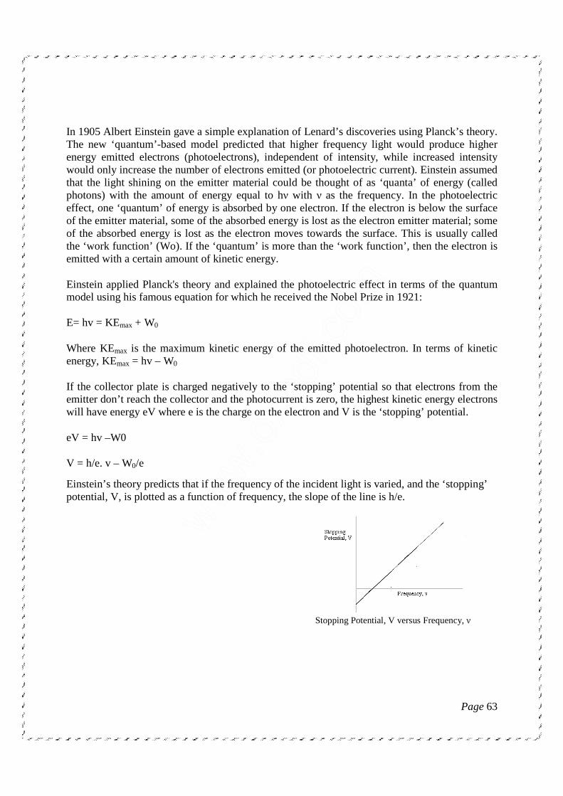
Page 63
In 1905 Albert Einstein gave a simple explanation of Lenard’s discoveries using Planck’s theory. The new ‘quantum’-based model predicted that higher frequency light would produce higher energy emitted electrons (photoelectrons), independent of intensity, while increased intensity would only increase the number of electrons emitted (or photoelectric current). Einstein assumed that the light shining on the emitter material could be thought of as ‘quanta’ of energy (called photons) with the amount of energy equal to hν with ν as the frequency. In the photoelectric effect, one ‘quantum’ of energy is absorbed by one electron. If the electron is below the surface of the emitter material, some of the absorbed energy is lost as the electron emitter material; some of the absorbed energy is lost as the electron moves towards the surface. This is usually called the ‘work function’ (Wo). If the ‘quantum’ is more than the ‘work function’, then the electron is emitted with a certain amount of kinetic energy.
Einstein applied Planck's theory and explained the photoelectric effect in terms of the quantum model using his famous equation for which he received the Nobel Prize in 1921:
E= hv = KEmax + W0
Where KEmax is the maximum kinetic energy of the emitted photoelectron. In terms of kinetic energy, KEmax = hv – W0
If the collector plate is charged negatively to the ‘stopping’ potential so that electrons from the emitter don’t reach the collector and the photocurrent is zero, the highest kinetic energy electrons will have energy eV where e is the charge on the electron and V is the ‘stopping’ potential.
eV = hv –W0
V = h/e. v – W0/e
Einstein’s theory predicts that if the frequency of the incident light is varied, and the ‘stopping’ potential, V, is plotted as a function of frequency, the slope of the line is h/e.
Stopping Potential, V versus Frequency, ν

Page 64
PRINCIPLE OF EXPERIMENT:
When incident light shines on the cathode (K), photoelectrons are emitted and transferred to the anode (A).This constitutes a photocurrent. By changing the voltage between the Anode and Cathode, and measuring the photocurrent, you can determination of the current-voltage curves of the photoelectric tube. The photocurrent is zero when the voltage between the cathode and anode is equal to the stopping potential. The slope of a plot of stopping potential versus frequency is the value of the ratio h/e.
The basic facts of the photoelectric effect experiments are as follows:
• For a given frequency (colour) of light, if the voltage between the cathode and anode,VAK, is equal to the stopping potential, V, the photocurrent is zero.
• When the voltage between the cathode and anode is greater than the stopping voltage, the photocurrent will increase quickly and eventually reach saturation. The saturated current is proportional to the intensity of the incident light. See Figure 2.
• Light of different frequencies (colors) have different stopping potentials. See Figure 3.
• The slope of a plot of stopping potential versus frequency is the value of the ratio, h/e. See Figure 1.
• The photoelectric effect is almost instantaneous. Once the light shines on the cathode, photoelectrons will be emitted in less than a nanosecond.

Page 65
BASIC SETUP Install the Mercury Lamp in the Mercury Light Source Enclosure • Use a Phillips head screwdriver to remove the four small screws that hold the back plate on to the Mercury Light Source enclosure. •Use a small flat-blade screwdriver to pry the back panel off of the enclosure.
•Screw the mercury lamp into the socket inside the enclosure. •Replace the back panel and screws on the enclosure. Alignment screws The Mercury Light Source has two small alignment screws on opposite corners of its base. The Photodiode enclosure has slightly larger alignment screws installed along the midline of its base. Mount the Enclosures on the Base Place the Mercury Light Source enclosure on the base so that the alignment screws go into the matching alignment holes on the base, and the position indicator arrow on the side of the enclosure is aligned with 0 mm on the edge of the base. Place the Photodiode enclosure on the base so that the alignment screws go into the matching alignment holes on the slot in the base, and the position indicator arrow on the side of the enclosure is aligned with 400 mm on the edge of the base Connect Cords and Cables Note: Before connecting any cords or cables, be sure that both switches on the h/e Power Supply are in the OFF position. •Connect the power cord from the Mercury Light Source enclosure into the receptacle labeled “POWER OUTPUT FOR MERCURY ~220V” on the side of the h/e Power Supply. •Connect the special DIN-plug-to-DIN-plug power cable between the port on the back of the Photoelectric Effect Apparatus labeled “POWER SUPPLY” and the port on the h/e Power Supply labeled “POWER OUTPUT FOR APPARATUS”. Screw the knurled rings on the plug ends of the cable onto the threaded section of each port. •Connect the special BNC-plug-to-BNC-plug cable between the port marked “K” on the Photodiode Enclosure and the port marked “K” on the back of the Photoelectric Effect Apparatus. Screw the knurled rings on the plug ends of the cable onto the threaded section of each port.
Note: Do not touch the glass envelope of the mercury lamp. Oil and moisture from the skin may diminish the lamp’s performance. Use gloves, a clean cloth, or a paper towel to handle the mercury lamp.

Page 66
•Connect the red banana-plug patch cord between the port marked “A” on the Photodiode enclosure and the port marked “A” on the back of the Photoelectric Effect Apparatus. •Connect the blue banana-plug patch cord between the port marked with the ‘down arrow’ (symbol for GROUND) on the Photodiode enclosure and the port marked with the ‘down arrow’ (GROUND) on the back of the photoelectric Effect Apparatus. •Connect the power cord between the port on the side of the h/e Power Supply labeled “POWER INPUT ~110V” and an appropriate electrical outlet (Note: For the 220 volt model, connect the cord between the port labeled “POWER INPUT ~220V” and an appropriate electrical outlet.) Note: These three cords will be disconnected during calibration. You do not need to turn off the power from power supply when you disconnect and then reconnect these three cords. h/e Photoelectric Effect Apparatus The h/e Photoelectric Effect Apparatus has four knobs, three buttons and two digital displays on its front panel, and four ports (labeled A, K, ‘down arrow’, and POWER SUPPLY) on its back panel. The apparatus measures the photocurrent through the photodiode tube and the voltage across the photodiode tube.
• Current Range switch: Sets the current range for the instrument’s current amplifier (10-8 to 10-13 A).
• Ammeter: Displays the photocurrent through the photodiode tube. • Voltmeter: Displays potential across the photodiode tube. • Voltage Range switch: Sets the voltage range as -2 to +30 V for plotting current-voltage
characteristics and -2 to +2 V for measuring the stopping potential. • Power switch: Turns the power to the instrument ON or OFF. • Voltage Adjust: Sets the potential across the photodiode tube for both voltage ranges. • Current Calibration: Sets the current through the instrument to zero. • Phototube Signal switch: Sets the signal from the photodiode tube to CALIBRATION or
MEASURE. Measurement Accuracy Two factors may affect the measurement accuracy. First, the photocurrent is extremely small. Second, because of the cathode dark current and the anode reverse current, the voltage when the photocurrent is zero is not exactly the stopping potential. (For more information, see Experiments in Modern Physics by A. Melissinos, copyright 1966, Harcourt Brace Jovanovich, publishers.) The apparatus has a very sensitive and stable current amplifier so that the small photocurrent can be measured accurately. The photodiode tube has a low level of dark current and anode reverse voltage. In addition, because stopping potential versus frequency is plotted for several spectral lines and the slope of stopping potential versus frequency is used to calculate Planck’s constant, the slope method gives an accurate result even if the stopping potential is not exactly accurate.

Page 67
MEASURING AND CALCULATING PLANCK’S CONSTANT, h PREPARATION BEFORE MEASUREMENT
3. Cover the window of the Mercury Light Source enclosure with the Mercury Lamp Cap from the Optical Filters box. Cover the window of the Photodiode enclosure with the Photodiode Cap from the Optical Filters box.
4. On the h/e Power Supply, turn on POWER and MERCURY LAMP. On the Photoelectric Effect Apparatus, push in the POWER button to the ON position.
5. Allow the light source and the apparatus to warm up for 20 minutes.
6. On the apparatus, set the VOLTAGE to –2 — +2 V. Turn the CURRENT RANGES
switch to 10-13 7. To set the current amplifier to zero, first disconnect the ‘A’, ‘K’, and ‘down arrow’
(GROUND) cables from the back panel of the apparatus. 8. Press the PHOTOTUBE SIGNAL button in to CALIBRATION. 9. Adjust the CURRENT CALIBRATION knob until the current is zero. 10. Press the PHOTOTUBE SIGNAL button to MEASURE. 11. Reconnect the ‘A’, ‘K’, and ‘down arrow’ (GROUND) cables to the back of the
apparatus.
MEASUREMENT
1. Uncover the window of the Photodiode enclosure. Place the 4 mm diameter aperture
and the 365 nm filter onto the window of the enclosure. (See the sidebar note.)
2. Uncover the window of the Mercury Light Source. Spectral lines of 365 nm wavelength will shine on the cathode in the phototube.
3. Adjust the VOLTAGE ADJUST knob until the current on the ammeter is zero.
4. Record the magnitude of the stopping potential for the 365nm wavelength in table1.
5. Cover the window of the mercury light source.
6. Replace the 365 nm filter with the 405 nm filter.
Note: It is very important to allow the light source and apparatus to warm up for 10 minutes prior to making any measurements.

Page 68
7. Uncover the window of the Mercury Light Source. Spectral lines of 405 nm wavelength will shine on the cathode in the phototube.
8. Adjust the VOLTAGE ADJUST knob until the current on the ammeter is zero.
9. Record the magnitude of the stopping potential for the 405 nm wavelength in Table 1.
10. Cover the window of the Mercury Light Source.
11. Repeat the measurement procedure for the other filters. Record the magnitude of the
stopping potential for each wavelength in Table 1.
OBSERVATION TABLE
Observation for Stopping Potential of Spectral Lines, 4 mm diameter aperture. S.No. Wavelength, λ (nm) Frequency
ν = c/ λ, (x 1014 Hz) Stopping Potential, V (Volt)
1. 365.0 8.214 2. 405.0 7.408 3. 436.0 6.879 4. 546.0 5.490 5. 577.0 5.196
Repeat observation for 2 mm and 8 mm diameter apertures.
CALCULATION
1. Plot a graph of Stopping Potential (V) versus Frequency (x 1014 Hz).
2. Find the slope of the best-fit line through the data points on the Stopping Potential
(V) versus Frequency (x 1014 Hz) graph. Note: The slope is the ratio of h/e, so Planck’s constant, h, is the product of the charge of the electron (e = 1.602 x10⁻¹⁹ C) and the slope of the best-fit line. According to the theory of linear regression, the slope of the Stopping Potential versus Frequency graph can be calculated using the following equation:

Page 69
where
3. Record the calculated slope and use it to calculate the value of Planck’s constant, h. Slope = ……………………….. h = e x slope = …………………………
4. Estimate the error in the slope and round your result to the appropriate value. Compare your calculated value of h to the accepted value, h0, 6.626 x 10⁻³⁴ J s.
h - h0 Percent difference = x 100
h0
5. Record your percent difference ______________________ QUESTIONS
1. How does your calculated value of h compare to the accepted value? 2. What do you think may account for the difference – if any – between your calculated
value of h and the accepted value? 3. How can you find the value of the Work Function from the graph of Stopping Potential
versus Frequency? Extension Repeat the data measurement and analysis procedure for the other two apertures in the OPTICAL FILTERS box Table 2: .Stopping Potential of Spectral Lines, 2 mm diameter Aperture Table 3: .Stopping Potential of Spectral Lines, 8 mm diameter Aperture.
Questions 1. How does your calculated value of h for each different aperture compare to the accepted
value,h0, 6.626 x 10⁻³⁴ J s? 2. How does light intensity affect the Stopping potential?

Page 70
EXPERIMENT EXPERIMENT EXPERIMENT EXPERIMENT 11112222::::
COUPLED PENDULUMCOUPLED PENDULUMCOUPLED PENDULUMCOUPLED PENDULUM
AIMS/ OBJECT: Study of coupled oscillations. APPARATUS USED:
1. Pendulum rods 2. Stop watch 3. Helical spring with two eyelets, 3N/m 4. Table clamps 5. Universal clamps 6. Stainless steel rods, 1000mm
PRINCIPLE: For oscillation of two coupled pendulums, the oscillation energy is transferred from one pendulum to other and back again. If the two pendulums are identical and the oscillation is started from a position where one is suspended in its rest position while the other is at a point of maximum deflection, then all the energy in the system is transferred between the pendulums. i.e. one pendulum always comes to rest while the other is swinging at its maximum amplitude. The time between two such occurrences of rest for one pendulum or more generally, the time between any two instances of minimum amplitude is referred to as the beat period. T. The oscillation of two identical coupled pendulums can be regarded as a superimposition of two natural oscillations. These natural oscillations can be observed when the both pendulums are fully in phase or fully out of phase. In the first case both pendulums vibrate at the frequency that they would if the coupling to the other pendulum were not present at all. In the second case, the effect of the coupling is at a maximum and the inherent frequency is greater. All other oscillations can be described by superimposing these two natural oscillations. The equation of motion for the pendulums (for small angles of deflection φ1 and φ2) takes the form: L. φ1 + g. φ1+k.( φ1 - φ2) =0 L. φ2 + g. φ2+k.( φ2 – φ1) =0 Where: g : acceleration due to gravity, L : length of pendulum, k : coupling constant φ1 = φ2= φ -φ1 = φ2= φ φ1 φ2 φ φ -φ φ General coupled oscillation Coupled oscillation in phase Coupled oscillation out of phase

Page 71
For the motions ϕ+ = ϕ1 + ϕ2 and ϕ-− = ϕ1 – ϕ2 (initially chosen arbitrarily) the equation of motion is as follows: L.ϕ+ +g. ϕ+ =0 L.ϕ- +(g+2k). ϕ- =0 (2) The solutions ϕ+ =a+ cos (ω+t) + b+sin(ω+t) ϕ- =a-cos (ω-t) + b-sin (ω-t) (3) give rise to angular frequencies ω+ = √ g/L and ω- = √ (g+2k)/L (4) Corresponding to the natural frequencies for in phase or out of phase motion (ϕ+ = 0 for out of phase motion and ϕ– = 0 for in-phase motion). The deflection of the pendulums can be calculated from the sum or the difference of the two motions, leading to the solutions ϕ1 = ½ (a+cos(ω+t) + b+sin(ω+t) + a-cos(ω-t) + b-sin(ω-t)) ϕ2 = ½ (a+cos(ω+t) + b+sin(ω+t) - a-cos(ω-t) - b-sin(ω-t)) (5) Parameters a+, a–, b+ and b– are arbitrary coefficients that can be calculated from the initial conditions for the two pendulums at time t = 0. The easiest case to interpret is where pendulum 1 is deflected by an angle ϕ0 from its rest position and released at time 0 while pendulum 2 remains in its rest position. ϕ1 = ½ (ϕ0.cos (ω+t) + ϕ0.sin (ω-t) ϕ2 = ½ (ϕ0.cos (ω+t) - ϕ0.sin (ω-t) (6) After rearranging the equations they take the form ϕ1 = ϕ0.cos (ωΔt). cos (ωt) ϕ1 = ϕ0.sin (ωΔt). cos (ωt) (7) With ωΔ = (ω- - ω+)/2 ω = (ω+ + ω-)/2 (8) This corresponds to an oscillation of both pendulums at identical angular frequency ω, where the amplitudes are modulated at an angular frequency ω∆. This kind of modulation results in beats. In the situation described, the amplitude of the beats arrives at a maximum since the overall amplitude falls to a minimum at zero.

Page 72
Fig. 2: Set-up for recording and evaluating the oscillation of two identical pendulums coupled together by a spring
The set-up is illustrated in Fig. 2.
• Clamp two stand rods of 1000 mm length to a bench so that they are about 15 cm apart.
• Attach a short stand rod between them as a horizontal cross member to lend the set-up more stability.
• Attach the angle sensors to the top of the vertical rods using universal clamps.
• Attach bobs to the end of the pendulum rods.
• Suspend the pendulum rods from the angle sensors (there are grooves in the angle sensors to accommodate the hinge pins of the pendulum rods).
• Attach the spring via the holes in the pendulum rods. These are about 40 cm from the fulcrum of the pendulum.
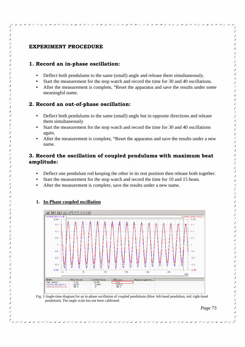
Page 73
EXPERIMENT PROCEDURE 1. Record an in-phase oscillation:
• Deflect both pendulums to the same (small) angle and release them simultaneously. • Start the measurement for the stop watch and record the time for 30 and 40 oscillations. • After the measurement is complete, “Reset the apparatus and save the results under some
meaningful name. 2. Record an out-of-phase oscillation:
• Deflect both pendulums to the same (small) angle but in opposite directions and release them simultaneously
• Start the measurement for the stop watch and record the time for 30 and 40 oscillations again.
• After the measurement is complete, “Reset the apparatus and save the results under a new name.
3. Record the oscillation of coupled pendulums with maximum beat amplitude:
• Deflect one pendulum rod keeping the other in its rest position then release both together. • Start the measurement for the stop watch and record the time for 10 and 15 beats. • After the measurement is complete, save the results under a new name.
1. In-Phase coupled oscillation
Fig. 3 Angle-time diagram for an in-phase oscillation of coupled pendulums (blue: left-hand pendulum, red: right-hand pendulum). The angle scale has not been calibrated.

Page 74
2. Out of Phase coupled oscillation
Fig. 4 Angle-time diagram for an out-of-phase oscillation of coupled pendulums (blue: left-hand pendulum, red: right-hand pendulum). The angle scale has not been calibrated.
3. Oscillation of coupled pendulums with maximum beat amplitude
Fig. 5 Angle-time diagram for an oscillation of coupled pendulums with maximum beat amplitude (blue: left-hand pendulum, red: right-hand pendulum). The angle scale has not been calibrated.
Fig. 6: Magnified view of one beat period in the oscillation of coupled pendulums with maximum beat amplitude (blue: left-hand pendulum, red: right-hand pendulum). The angle scale has not been calibrated.
Page 75
EVALUATION 1. Determine the period of oscillation for coupled pendulums oscillating in phase
• Open the data entry for the in-phase oscillation. • Calculate the time period in in-phase (T+). • And determine the frequency (ω+).
The period of the oscillation is the time divided by the number of complete oscillations included in that time T+ = total time / no. of complete oscillations 2. Determine the period of oscillation for coupled pendulums oscillating out of phase
• Open the data entry for the out-of-phase oscillation and proceed exactly as before. • Calculate the time period in out-phase (T-). • And determine the frequency (ω-).
The period of the oscillation is the time divided by the number of complete oscillations included in that time T– = total time / no. of complete oscillations 3. Determine the period of oscillation for coupled pendulums oscillating with maximum beat amplitude
• Open the data entry for the oscillation with the maximum beat amplitude. • Calculate the time period in beat (T∆). • And determine the frequency (ωΔ).
The period of the maximum beat amplitude is the time divided by the number of periods of the beat oscillation included in that time T∆ = 4. Compare the measurements for the two periods with the values as calculated from the intrinsic periods: For a coupled oscillation with a period T, where the beat amplitude is at its maximum, the expression below follows from equation (8): T = 2. [(T+.T-)/(T++T-) ] = 1,681s (9)

Page 76
Compare this with the measured value of T = 1.685 s. The beat period T∆ can also be calculated in a similar way. It should be noted, however, that this is usually defined to be the time between successive points where the pendulums stop still at the rest position. This actually represents only half the period of the underlying cosine or sine modulation term in equation (7). T∆ = (T+.T-) / (T+-T-) = 26 s (10) Compare this answer with the measured value of T∆ = 25 s . The difference of about one second between the calculated and measured values may seem to be quite large at first glance but it is due to the calculation being highly sensitive to differences between the intrinsic oscillation periods. If the intrinsic periods of the two pendulums differ by as little as 4 milliseconds, which roughly correspond to the maximum measurement accuracy achievable for the intrinsic oscillation periods in this experiment, it leads to a difference of a whole second in the beat period. 5. Determine the spring constant of the spring coupling the two pendulums The spring constant D of the spring coupling the pendulums is related to the coupling constant k as follows: D = k. (L /d2) .m (11) (d: distance between the point at which the spring is connected to the pendulum and the fulcrum of the pendulum) If the coupling is weak (k << g) the spring constant has little influence on the period of the out-of-phase oscillation but has a major influence on the beat period. Thus to calculate the spring constant, we relate it to the beat period by substituting equation (4) into (8) and rearranging to give k. K = 2. L. (ω∆
2 – ω∆ ω+) (12) Now the angular frequencies are replaced by the periods and substituted into equation (11) to give: D = (L /d2) .m. g/2.{2. (T+/ T∆) + (T+
2/ T∆2)} = 3, 5 N/m (13)