fit department of electrical engineering seminarmy.fit.edu/seces/slides/44.pdf · fit department of...
TRANSCRIPT
FIT Department of Electrical
Engineering Seminar
Adrian M. Peter, PhD([email protected])
Academic Collaborators:Anand Rangarajan
University of Florida
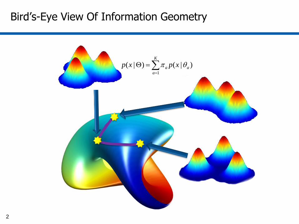
Bird’s-Eye View Of Information Geometry
K
a
aa xpxp1
)|()|(
2
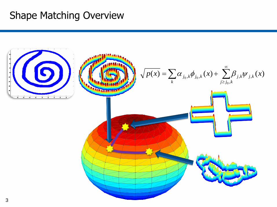
Shape Matching Overview
k kjj
kjkjkjkj xxxp,
,,,,
0
00)()()(
3

Agenda
Information Geometry
• Introduction
• Generalized Metrics
Wavelet Densities
• Maximum Likelihood Estimation
• Shape L’ÂneRouge
Applications
• Text Mining, Cyber
• Future Research
4
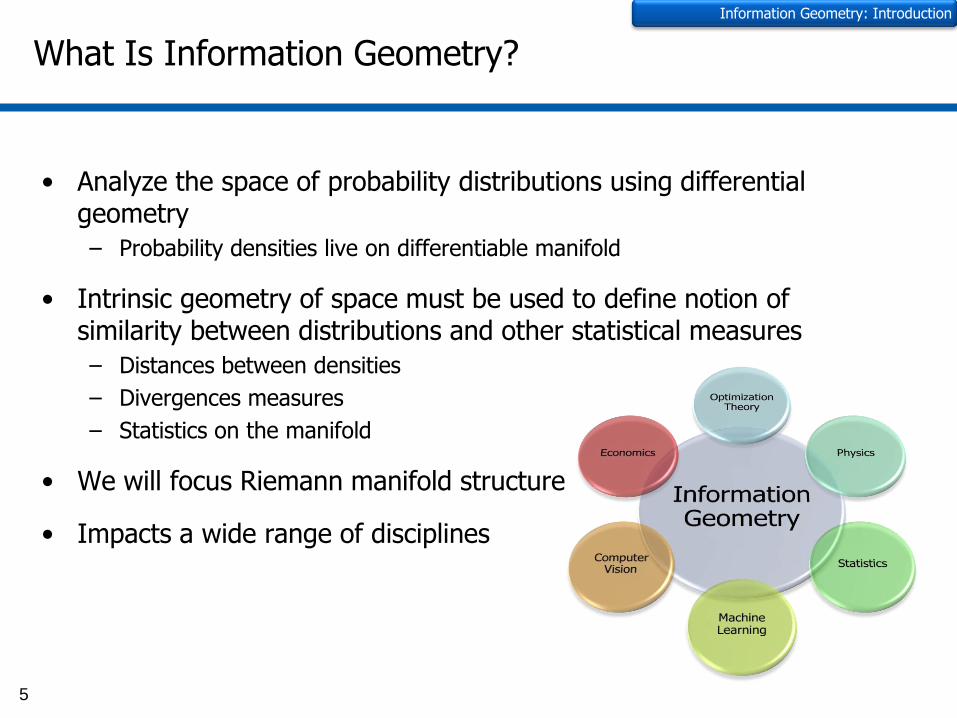
What Is Information Geometry?
• Analyze the space of probability distributions using differential geometry
– Probability densities live on differentiable manifold
• Intrinsic geometry of space must be used to define notion of similarity between distributions and other statistical measures
– Distances between densities
– Divergences measures
– Statistics on the manifold
• We will focus Riemann manifold structure
• Impacts a wide range of disciplines
5
Information Geometry: Introduction

Modus Operandi: Assume Flatness
• Euclidean space assumption dominates scientific landscape
• What happens when the elements of analysis live on curved space?
6
Information Geometry: Introduction
22212 dddddsT
1
2
1d
2d
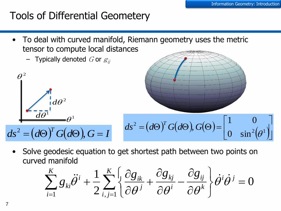
Tools of Differential Geometery
• To deal with curved manifold, Riemann geometry uses the metric tensor to compute local distances
– Typically denoted G or gij
• Solve geodesic equation to get shortest path between two points on curved manifold
7
Information Geometry: Introduction
IGdGddsT
,2
1
2
1d
2d
12
2
sin0
01 ,
GdGdds
T
1 , 1
10
2
K Kkj iji i jik
kik j i ki i j
g gE gg
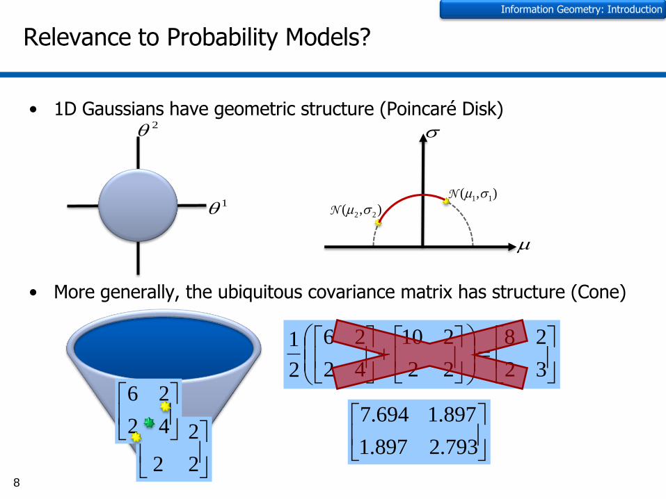
• 1D Gaussians have geometric structure (Poincaré Disk)
• More generally, the ubiquitous covariance matrix has structure (Cone)
32
28
22
210
42
26
2
1
22
210
42
26
Relevance to Probability Models?
8
Information Geometry: Introduction
1
2
793.2897.1
897.1694.7
),( 11 N
),( 22 N

Information Metrics
• Rao [3] established that Fisher information matrix was a Riemannian metric between densities of parametric families
• Model parameters are local coordinates of the manifold
For GMM
Probabilistic Manifold Dim = 2K
log ( | ) log ( | )( ) ( | )ij i j
p pg p d
x Θ x Θ
Θ x Θ x
Information Geometry: Introduction
K
a
aa xpxp1
,11 )|()|(
K
a
aa xpxp1
,22 )|()|(
2
3
1
3
2
2
1
2
2
1
1
1
6
5
4
3
2
1

Why Fisher Information Matrix?
• Close relationship to KL-divergence
• Invariance under “smooth” mappings of input space random variable (covariant under transformations of parameters)
• Cramér–Rao: lower bound on the variance of an unbiased parameter estimator
10
Information Geometry: Introduction
GppKL T
2
1)(||)(
)()(
)|()|(J ,)(
ygxg
xpypxfy
ijij
iii G 1)ˆ(Var

Beyond Fisher Information
• Do we always have to use the Fisher information matrix?
• Computational difficulties with Fisher-Rao metric tensor
– Not possible to get closed-form
• Our motivation - simple form of the metric tensor (also valid Riemannian metric):
• For Gaussian mixtures, above form enables separable 1D Gaussian integrations and closed-form solutions
– Note: closed-form is for gij not geodesic
– Only means of mixture components considered as coordinates for manifold (i.e. fixed covariances)
( | ) ( | )( )ij i j
p pg d
x Θ x Θ
Θ x
Information Geometry: Generalized Metrics

Generalized Entropy Leads To New Metrics
• Generalized φ-entropy (Burbea and Rao [1])
• Under this generalized entropy, the metric tensor becomes
• Setting φ(p)=p log(p) results in the Shannon entropy and consequently the Fisher information matrix
2R
( ) ( )H p p d x
( ) ( )ij i j
p pg p d
Θ x
Information Geometry: Generalized Metrics

α -Order Entropy Metrics
• Havrda and Charvát [2] α-order entropy uses
• We let α=2, which results in
• Still in early stages of investigating properties of new metric
• Door is open for development of more application specific information metrics
1( ) ( 1) ( ), 1p p p
1( ) 1
2p
Information Geometry: Generalized Metrics
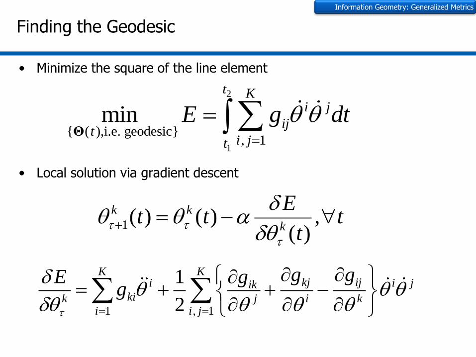
Finding the Geodesic
• Minimize the square of the line element
• Local solution via gradient descent
2
1
{ ( ),i.e. geodesic}, 1
min
t Ki j
ijt
i jt
E g dt
Θ
1( ) ( ) ,( )
k k
k
Et t t
t
1 , 1
10
2
K Kkj iji i jik
kik j i ki i j
g gE gg
Information Geometry: Generalized Metrics
Wavelet Density Estimation

Wavelet Representations
• Wavelets can approximate any f∊ℒ2, i.e.
• Only work with compactly supported, orthogonal basis families: Haar, Daubechies, Symlets, Coiflets
Wavelet Densities: Maximum Likelihood Estimation
k kjj
kjkjkjkj xxxf,
,,,,
0
00)()()(
Translation index Resolution level
Father Mother
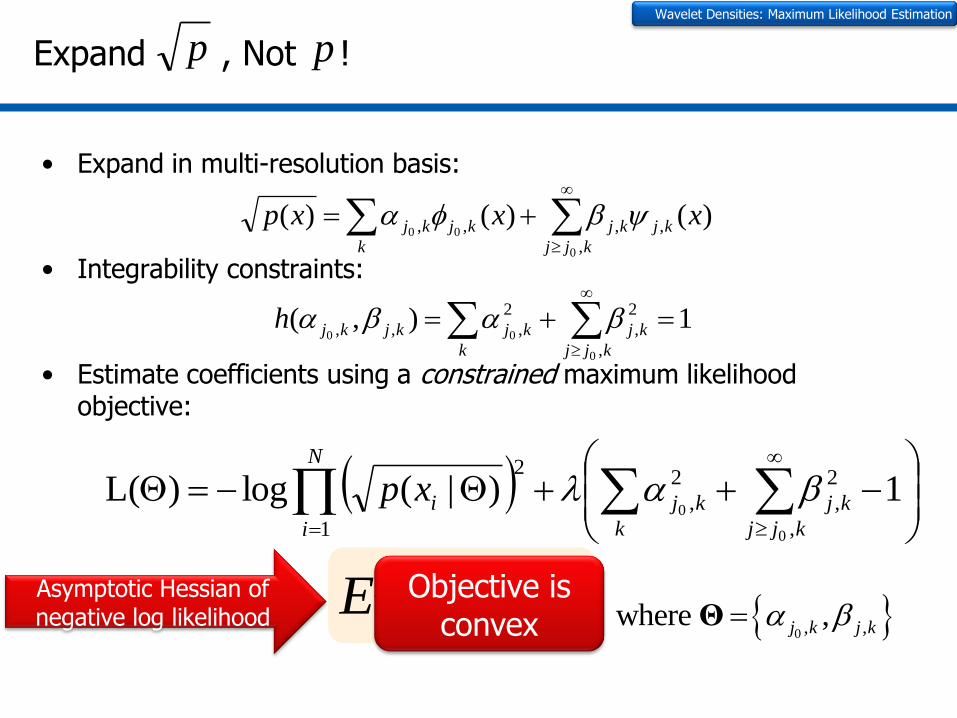
Expand , Not !
• Expand in multi-resolution basis:
• Integrability constraints:
• Estimate coefficients using a constrained maximum likelihood objective:
Wavelet Densities: Maximum Likelihood Estimation
p p
k kjj
kjkjkjkj xxxp,
,,,,
0
00)()()(
1),(,
2
,
2
,,,
0
00
k kjj
kjkjkjkjh
0 , ,where ,j k j k Θ
1)|(log)(L,
2
,
2
,
1
2
0
0
k kjj
kjkj
N
i
ixp
IH 4LEAsymptotic Hessian of negative log likelihood
Objective is convex

Modified Newton’s Method for L(Θ)
• General form
• Implemented by solving
• Iterative update equations
• Good convergence properties.
Wavelet Densities: Maximum Likelihood Estimation
hh
hT
LL
1
1
1
0
H
B
hdh
yhdT
LB
y
d
1
1
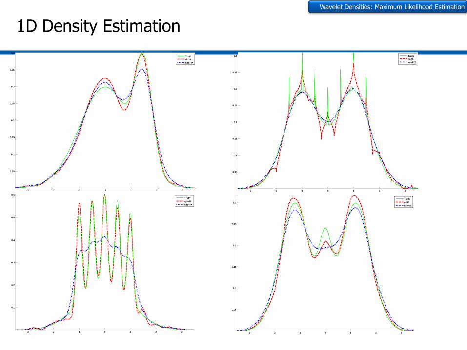
1D Density Estimation
-3 -2 -1 0 1 2 3
0.1
0.2
0.3
0.4
0.5
0.6
Best claw using sym10, Level = 2 error type: ISE
Truth
sym10
kdeFIX
-3 -2 -1 0 1 2 3
0.05
0.1
0.15
0.2
0.25
0.3
Best tri using coif3, Level = 1 error type: ISE
Truth
coif3
kdeFIX
-3 -2 -1 0 1 2 3
0.05
0.1
0.15
0.2
0.25
0.3
0.35
0.4
Best skewedBi using db10, Level = 1 error type: ISE
Truth
db10
kdeFIX
-3 -2 -1 0 1 2 3
0.05
0.1
0.15
0.2
0.25
0.3
0.35
0.4
Best dblClaw using coif1, Level = 2 error type: ISE
Truth
coif1
kdeFIX
Wavelet Densities: Maximum Likelihood Estimation

2D Density Estimation
Density WDE KDE
Basis ISE Fixed BW ISE
Variable BW ISE
Bimodal SYM7 6.773E-03 1.752E-02 8.114E-03
Trimodal COIF2 6.439E-03 6.621E-03 1.037E-02
Kurtotic COIF4 6.739E-03 8.050E-03 7.470E-03
Quadrimodal COIF5 3.977E-04 1.516E-03 3.098E-03
Skewed SYM10 4.561E-03 8.166E-03 5.102E-03
Wavelet Densities: Maximum Likelihood Estimation
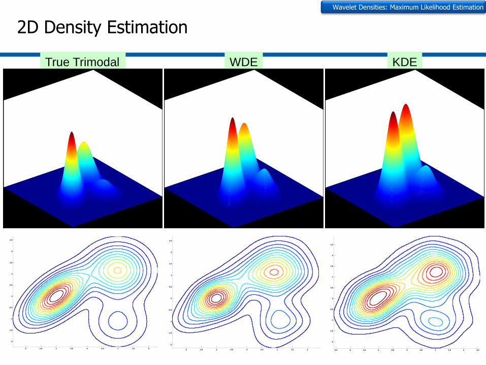
2D Density Estimation
WDE
-2 -1.5 -1 -0.5 0 0.5 1 1.5 2
-2
-1.5
-1
-0.5
0
0.5
1
1.5
2
2.5
KDE
-2.5 -2 -1.5 -1 -0.5 0 0.5 1 1.5 2 2.5
-2
-1.5
-1
-0.5
0
0.5
1
1.5
2
2.5
True Trimodal
-2 -1.5 -1 -0.5 0 0.5 1 1.5 2
-2
-1.5
-1
-0.5
0
0.5
1
1.5
2
2.5
Wavelet Densities: Maximum Likelihood Estimation

Image and Shape Applications
• Mutual information based registration (images from [22])
• Shape alignment using Hellinger divergence
Wavelet Densities: Maximum Likelihood Estimation
k kjj
kjkjkjkj
H dxppppD
,
)2(
,
)1(
,
)2(
,
)1(
,
2
2111
0
00
),(

Shape L’Âne RougeShape Matching With Sliding Wavelets

Shape L’Âne Rouge: Sliding Wavelets
Wavelet Densities: Shape L’Âne Rouge
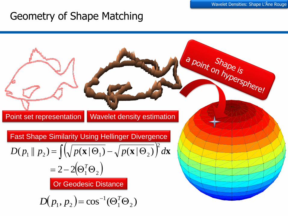
Geometry of Shape Matching
Wavelet density estimationPoint set representation
Wavelet Densities: Shape L’Âne Rouge
Or Geodesic Distance
)(cos, 21
1
21 TppD
Fast Shape Similarity Using Hellinger Divergence
21
2
2121
22
)|()|()||(
T
dppppD xxx
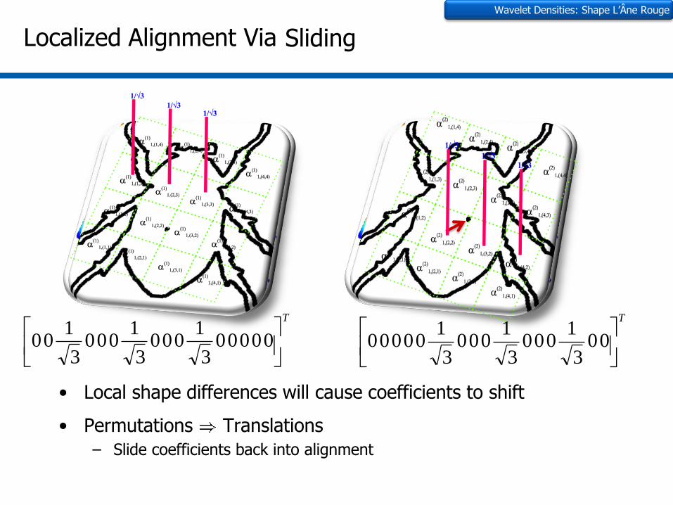
Localized Alignment Via
• Local shape differences will cause coefficients to shift
• Permutations Translations
– Slide coefficients back into alignment
Wavelet Densities: Shape L’Âne Rouge
Sliding
T
00000
3
1000
3
1000
3
100
T
00
3
1000
3
1000
3
100000
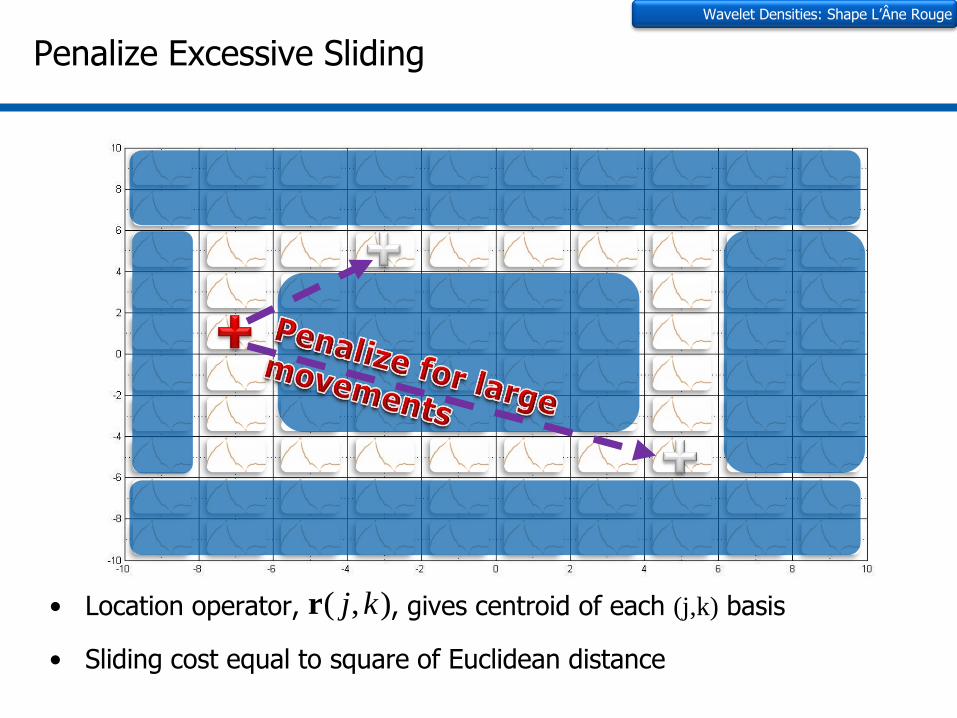
Penalize Excessive Sliding
• Location operator, , gives centroid of each (j,k) basis
• Sliding cost equal to square of Euclidean distance
Wavelet Densities: Shape L’Âne Rouge
),( kjr

Sliding Objective
• Objective minimizes over penalized permutation assignments
• Solve via linear assignment using cost matrix
– where Θi is vectorized list of ith shape’s coefficients and D is the matrix of
distances between basis locations.
Wavelet Densities: Shape L’Âne Rouge
kjj
kjkj
kj
kjkjE,
)2(
)(,
)1(
,
,
)2(
)(,
)1(
,
00
00
kjkj
kjkjkjkj,
2
,
2
00 ),(,),(,0
rrrr
DC T 21

Effects of λ
Wavelet Densities: Shape L’Âne Rouge
λ=10 λ=500 λ=1000
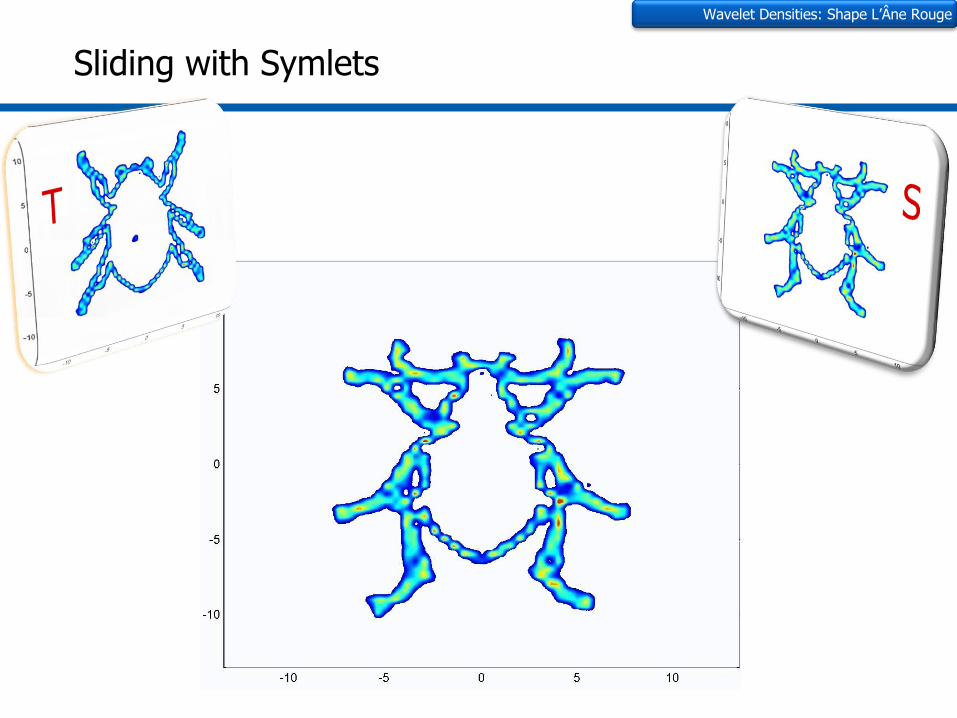
Sliding with Symlets
Wavelet Densities: Shape L’Âne Rouge

Recognition Results on MPEG-7 DB
Wavelet Densities: Shape L’Âne Rouge
• All recognition rates are based on MPEG-7 bulls-eye criterion
• D2 shape distributions (Osada et al. [11]) only at 59.3%

Related Work
• A few methods are reporting rates above 85%
– Shape-trees: 87.7% (Felzenszwalb-Schwartz [9], CVPR 2007)
– IDSC+EMD-L1: 86.56% (Ling-Okada [16], PAMI 2007)
– Hierarchical Procrustes: 86.35% (McNeill-Vijayakumar [8], CVPR 2006)
– IDSC + DP: 86.4% (Ling-Jacobs [7], CVPR 2005)
Wavelet Densities: Shape L’Âne Rouge
Criterion ST, HP, IDSC Shape L’ÂneRouge
No topologicalrestrictions
Large number ofpoints per shape
Computationally efficient
Accuracy
Applications of Information Geometry

Document Classification
• Carter et al. [17]
34
Information Geometry: Applications
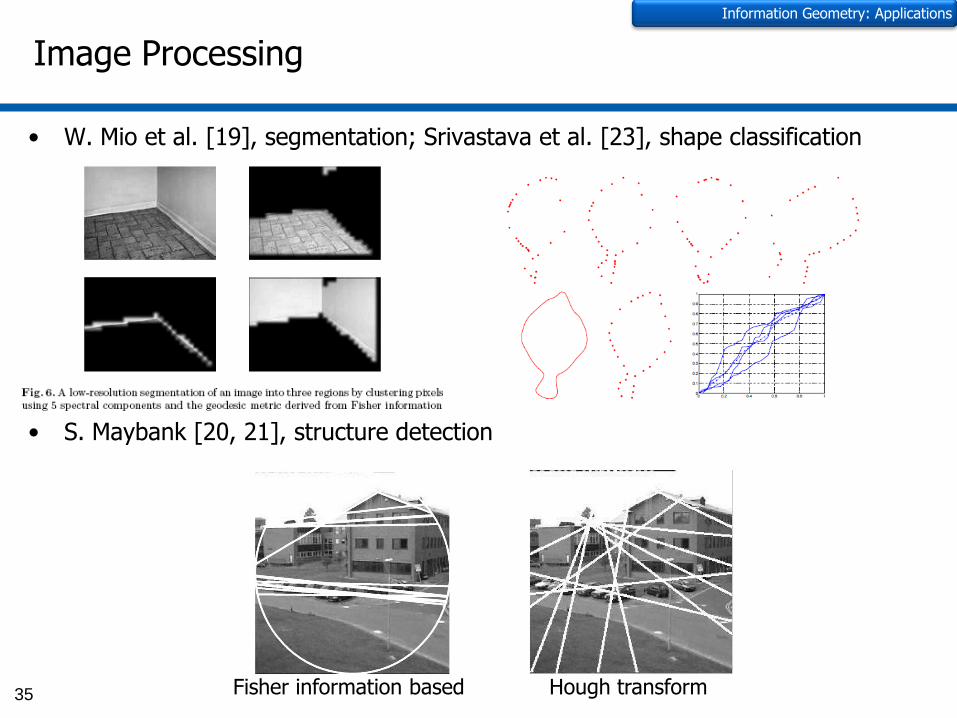
• W. Mio et al. [19], segmentation; Srivastava et al. [23], shape classification
• S. Maybank [20, 21], structure detection
Image Processing
35 Fisher information based Hough transform
Information Geometry: Applications
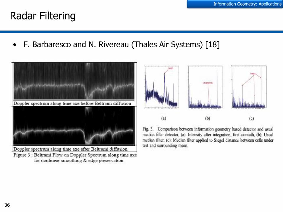
Radar Filtering
• F. Barbaresco and N. Rivereau (Thales Air Systems) [18]
36
Information Geometry: Applications
Current Investigations
• Cyber
– Return Oriented Programming attacks
– Exfiltration
• Semantic document matching
– Massive data clustering in a cloud environment (Hadoop)
• Incremental clustering of email content
– Complex Event Processing paradigm of doing clustering “on the wire”
• Signals intelligence
– Emitter identification
• Information Fusion
– Utilizing product manifold between families of distributions
37

Future Explorations for Research
• Look at connections with quantum mechanics
– Wave function’s related to model
• Derivation of other information metrics
• Modern computational approaches to numerically finding geodesics
– Employ GPUs
• Revisit probabilistic machine techniques to look at geometric implications
– Geodesic training of Markov Models?
• Collaborate with a variety of other disciplines 38
1)(2
dxx
p
Summary
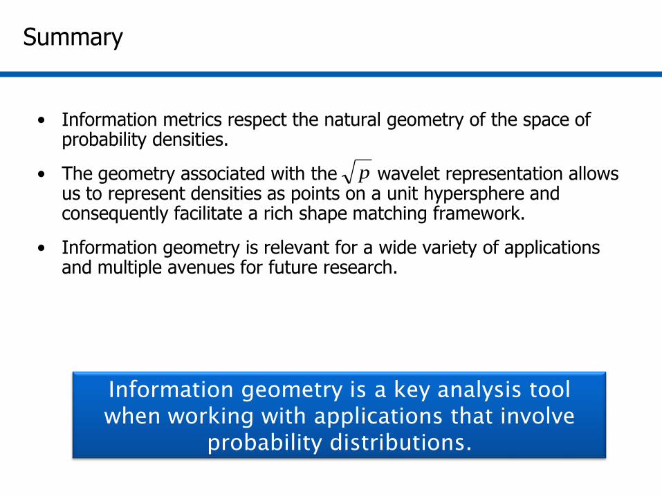
• Information metrics respect the natural geometry of the space of probability densities.
• The geometry associated with the wavelet representation allows us to represent densities as points on a unit hypersphere and consequently facilitate a rich shape matching framework.
• Information geometry is relevant for a wide variety of applications and multiple avenues for future research.
Information geometry is a key analysis tool
when working with applications that involve
probability distributions.
p
Relevant Publications for Shape Matching
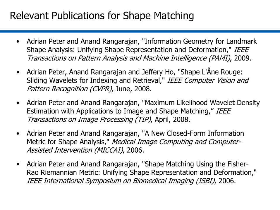
• Adrian Peter and Anand Rangarajan, "Information Geometry for Landmark Shape Analysis: Unifying Shape Representation and Deformation," IEEE Transactions on Pattern Analysis and Machine Intelligence (PAMI), 2009.
• Adrian Peter, Anand Rangarajan and Jeffery Ho, "Shape L'Âne Rouge: Sliding Wavelets for Indexing and Retrieval," IEEE Computer Vision and Pattern Recognition (CVPR), June, 2008.
• Adrian Peter and Anand Rangarajan, "Maximum Likelihood Wavelet Density Estimation with Applications to Image and Shape Matching,” IEEE Transactions on Image Processing (TIP), April, 2008.
• Adrian Peter and Anand Rangarajan, "A New Closed-Form Information Metric for Shape Analysis," Medical Image Computing and Computer-Assisted Intervention (MICCAI), 2006.
• Adrian Peter and Anand Rangarajan, "Shape Matching Using the Fisher-Rao Riemannian Metric: Unifying Shape Representation and Deformation," IEEE International Symposium on Biomedical Imaging (ISBI), 2006.

42

43
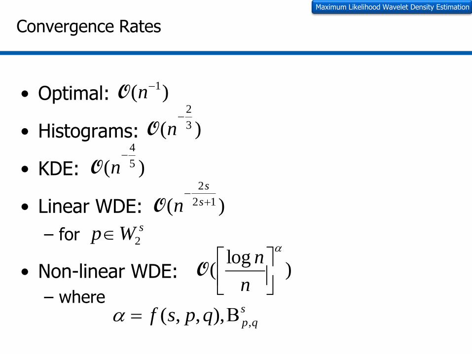
Convergence Rates
• Optimal:
• Histograms:
• KDE:
• Linear WDE:
– for
• Non-linear WDE:
– where
Maximum Likelihood Wavelet Density Estimation
)( 1nO
)( 3
2
nO
)( 5
4
nO
)( 12
2
s
s
nOsWp 2
)log
(
n
nO
s
qpqpsf ,),,,(

Why Fisher Information Matrix?
• Close relationship to KL-divergence
• Invariance under “smooth” mappings of input space random variable (covariant under transformations of parameters)
45
Information Geometry: Introduction
GppKL T
2
1)(||)(
dyypyp
g
dxypyp
dxxpxp
g
xpypxfy
jiij
ji
jiij
)|()|(4~
J)|()|(
4
)|()|(4
)|()|(J ,)(
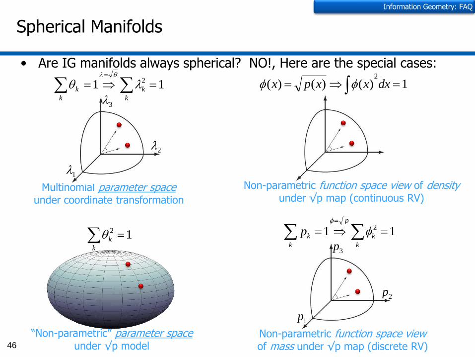
Spherical Manifolds
• Are IG manifolds always spherical? NO!, Here are the special cases:
46
12 k
k
“Non-parametric” parameter spaceunder √p model
Multinomial parameter spaceunder coordinate transformation
11 2
k
k
k
k
1
2
3
Information Geometry: FAQ
11 2
k
k
p
k
kp
1p
2p
3p
Non-parametric function space viewof mass under √p map (discrete RV)
1)()()(2
dxxxpx
Non-parametric function space view of densityunder √p map (continuous RV)

Model Selection

How Do We Select the Number of Levels?
• In the wavelet expansion of we need set j0 (starting level) and j1
(ending level)
• Balasubramanian [32] proposed geometric approach by analyzing the posterior of a model class
• The model selection criterion is
Model Selection: The Stochastic Complexity on Hyperspheres
p
k
j
kjj
kjkjkjkj xxxp1
0
00
,
,,,, )()()(
)(
)|()()()|(
Ep
dEpppEp
M
M
)ˆ(det
)ˆ(~detln
2
1)(detln)
2ln(
2)ˆ|(ln)M(
ij
ij
ijg
gdg
NkEpSC
ML fit Scales with
parameters and
samples.
Volume of model
class manifold
Ratio of expected Fisher
to empirical Fisher
)M(
)M(ln)ˆ|(ln)M(
ˆV
VEpSC
Total volume of manifold
Volume of distinguishable distributions around ML

Connections to MDL
• Volume around MLE
• Last term of razor disappears
• This simplification leads to
N
g
gI
ij
ij,1
)ˆ(~det
)ˆ(det)(
dgNk
EpMDLSC ij )(detln)2
ln(2
)ˆ|(ln)M(
2
1
2
ˆ)ˆ(~det
)ˆ(det2)(
ij
ij
k
g
g
NV
M
Model Selection: Stochastic Complexity on Hyperspheres

Geometric Intuition
Space of distributions Counting volumes
Model Selection: Stochastic Complexity on Hyperspheres

MDL for Wavelet Densities on the Unit Hypersphere
Model Selection: Stochastic Complexity on Hyperspheres
Space of distributions
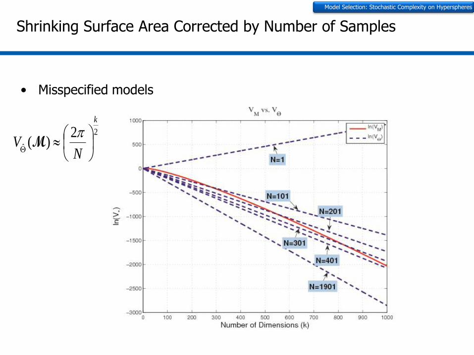
Shrinking Surface Area Corrected by Number of Samples
• Misspecified models
V
MV
MVV MVV
V
MV
2
ˆ
2)(
k
NV
M
Model Selection: Stochastic Complexity on Hyperspheres

Nested Subspaces Lead to Simpler Model Selection
• Hypersphere dimensionality remains the same with MRA
• It is sufficient to search over j0, using only scaling functions for density
estimation.
• MDL is invariant to MRA, however sparsity not considered.
k2
k
2
k
2
k
4
k
4
k
Model Selection: Stochastic Complexity on Hyperspheres
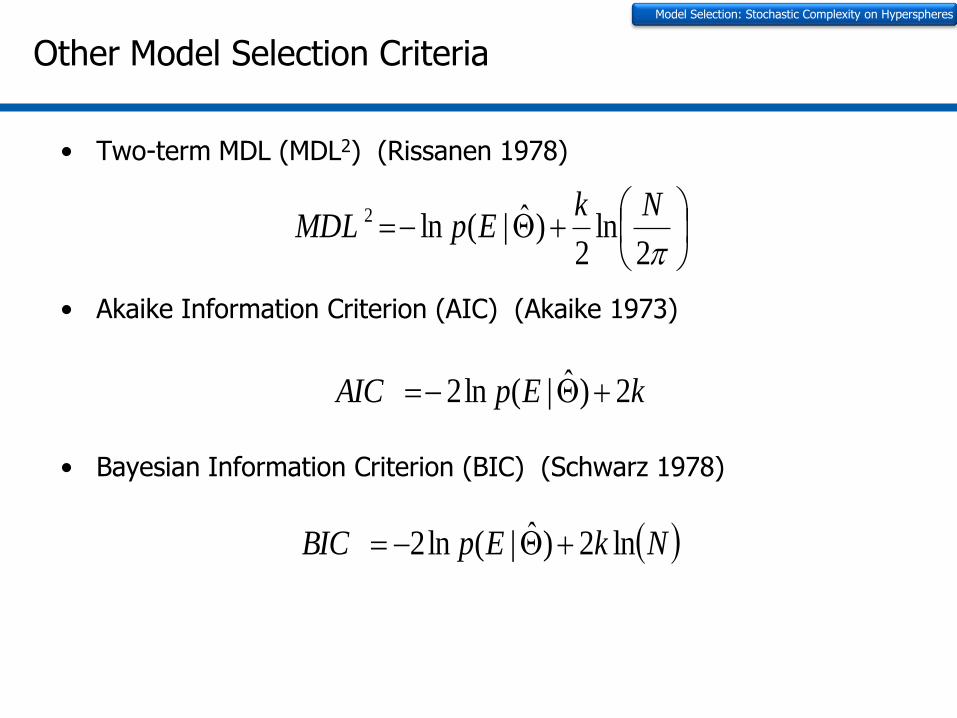
Other Model Selection Criteria
• Two-term MDL (MDL2) (Rissanen 1978)
• Akaike Information Criterion (AIC) (Akaike 1973)
• Bayesian Information Criterion (BIC) (Schwarz 1978)
2ln
2)ˆ|(ln2 Nk
EpMDL
kEpAIC 2)ˆ|(ln2
NkEpBIC ln2)ˆ|(ln2
Model Selection: Stochastic Complexity on Hyperspheres
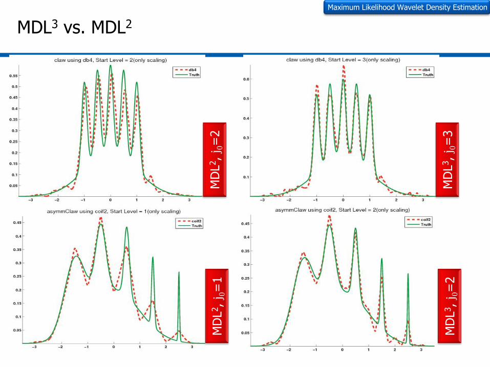
MDL3 vs. MDL2
Maximum Likelihood Wavelet Density Estimation
MD
L2,
j 0=
2
MD
L3,
j 0=
3
MD
L2,
j 0=
1
MD
L3,
j 0=
2

MDL3 vs. BIC and MSE
Maximum Likelihood Wavelet Density Estimation
BIC
, j 0=
0
MD
L3,
j 0=
1
MSE,
j 0=
4
MD
L3,
j 0=
2
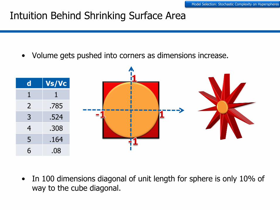
Intuition Behind Shrinking Surface Area
• Volume gets pushed into corners as dimensions increase.
• In 100 dimensions diagonal of unit length for sphere is only 10% of way to the cube diagonal.
d Vs/Vc
1 1
2 .785
3 .524
4 .308
5 .164
6 .08
Model Selection: Stochastic Complexity on Hyperspheres
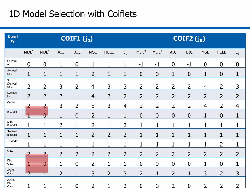
1D Model Selection with Coiflets
Density COIF1 (j0) COIF2 (j0)
MDL3 MDL2 AIC BIC MSE HELL L1 MDL3 MDL2 AIC BIC MSE HELL L1
Gaussian 0 0 1 0 1 1 1 -1 -1 0 -1 0 0 0Skewed Uni. 1 1 1 1 2 1 1 0 0 1 0 1 0 1Str. Skewed Uni. 2 2 3 2 4 3 3 2 2 2 2 4 2 3KurtoticUni. 2 2 2 1 4 2 2 2 2 2 2 2 2 2Outlier
2 2 3 2 5 3 4 2 2 2 2 4 2 4Bimodal
1 0 1 0 2 1 1 0 0 0 0 1 0 1Sep. Bimodal 1 1 2 1 2 1 2 1 1 1 1 1 1 1Skewed Bimodal 1 1 1 1 2 2 2 1 1 1 1 1 1 1Trimodal
1 1 1 1 1 1 1 1 1 1 1 1 2 1Claw
2 2 2 2 2 2 2 2 2 2 2 2 2 2Dbl. Claw 1 0 1 0 2 1 1 0 0 0 0 1 0 1Asym. Claw 2 1 2 1 3 2 3 2 1 2 1 3 2 3Asym. Dbl. Claw 1 1 1 0 2 1 2 0 0 2 0 2 2 2

2D Model Selection with Haar
Shape j0=-3 j0=-2 j0=-1 j0=0 j0=1 j0=2
MDL3, AIC
MDL2, BIC

References1. Burbea, J., Rao, R.: Entropy differential metric, distance and divergence measures in probability spaces: A unified approach. Journal of
Multivariate Analysis 12 (1982) 575–596
2. Havrda, M.E., Charvát, F.: Quantification method of classification processes: Concept of structural -entropy. Kybernetica 3 (1967) 30–35
3. Rao, C.: Information and accuracy attainable in estimation of statistical parameters. Bulletin of the Calcutta Mathematical Society 37 (1945) 81–91
4. A. Pinheiro and B. Vidakovic, “Estimating the square root of a densityvia compactly supported wavelets,” vol. 25, no. 4, pp. 399–415, 1997.
5. S. Penev and L. Dechevsky, “On non-negative wavelet-based density estimators,” Journal of Nonparametric Statistics, vol. 7, pp. 365–394.
6. D. Donoho, I. Johnstone, G. Kerkyacharian, and D. Picard, “Density estimation by wavelet thresholding,” Ann. Statist., vol. 24(2), pp. 508–539, 1996.
7. H. Ling and D. Jacobs. Using the inner-distance for classification of articulated shapes. In CVPR, 2005.
8. G. McNeill and S. Vijayakumar. Hierarchical procrustes matching for shape retrieval. In CVPR, 2006.
9. P.F. Felzenszwalb and J.D. Schwartz. Hierarchical Matching of Deformable Shapes. In CVPR, 2007.
10. Vijay Balasubramanian: Statistical Inference, Occam's Razor, and Statistical Mechanics on the Space of Probability Distributions. Neural Computation 9(2): 349-368 (1997)
11. R. Osada, T. Funkhouser, B. Chazelle, and D. Dobkin, “Shape distributions,” ACM Trans. on Graphics, no. 4, pp. 807–832, 2004.
12. G. Schwarz, Estimating the dimension of a model, The Annals of Statistics, vol. 6, no. 2, pp. 461464, 1978.
13. H. Akaike, Information theory and an extension of the maximum likelihood principle, in Proc. 2nd International Symposium on Information Theory, B. N. Petrov and F. Csaki, Eds., 1973, pp. 267281.
14. J. Rissanen, Modeling by shortest data description, Automatica, vol. 14, pp. 465471, 1978.
15. R. Jonker and A. Volgenant, A shortest augmenting path algorithm for dense and sparse linear assignment problems, Computing, vol. 38, pp. 325-340, 1987.
16. H. Ling and K. Okada, An Efficient Earth Mover's Distance Algorithm for Robust Histogram Comparison, PAMI, pp 840-853, 2007.
17. K. Carter, R. Raich, and A. Hero III, FINE: Information Embedding for Document Classification, ICASSP, 2008.
18. F. Barbaresco and N. Rivereau, Diffusive CFAR and its Extension for Doppler and Polarimetric Data, International Conference on Radar Systems, 2007.
19. W. Mio, D. Badlyans, X. Liu, A Computational Approach to Fisher Information with Applications to Image Analysis, EMMCVPR, 2005.
20. S. Maybank, Detection of Image Structures Using the Fisher Information and the Rao Metric, PAMI, 2004.
21. Ferryman, J. M. 2001 PETS’2001 database. (Available at http://www.visualsurveillance.org/PETS2001.)
22. BrainWeb database, http://www.bic.mni.mcgill.ca/brainweb/
23. Riemannian Analysis of Probability Density Functions with Applications in Vision , CVPR 2007.