Fluid-structure partitioned procedures based

on Robin transmission conditions

Santiago Badia a,b,∗, Fabio Nobile c, Christian Vergara c

aCIMNE, Universitat Politecnica de Catalunya, Jordi Girona 1-3, Edifici C1,08034 Barcelona, Spain

bComputational Mathematics and Algorithms, MS-1320, Sandia NationalLaboratories, Albuquerque, NM 87185-1320

cMOX - Dipartimento di Matematica “F. Brioschi” - Politecnico di Milano,Piazza Leonardo da Vinci 32, 20133 Milano, Italy

Abstract

In this article we design new partitioned procedures for fluid-structure interactionproblems, based on Robin-type transmission conditions. The choice of the coefficientin the Robin conditions is justified via simplified models. The strategy is effectivewhenever an incompressible fluid interacts with a relatively thin membrane, as inhaemodynamics applications. We analyze theoretically the new iterative procedureson a model problem, which represents a simplified blood-vessel system. In particular,the Robin-Neumann scheme exhibits enhanced convergence properties with respectto the existing partitioned procedures and does not need any relaxation. The Robin-

Robin scheme can further improve convergence if optimally tuned. The theoreticalresults are confirmed by numerical experimentation.

Key words: Fluid-structure interaction, partitioned procedures, transmissionconditions, Robin boundary conditions, added-mass effect, haemodynamics.

1 Introduction

In the last three decades, there has been an increasing interest in the sim-ulation of fluid-structure interaction (FSI) problems that appear in several

∗ Corresponding author.Email addresses: sbadia@cimne.upc.edu (Santiago Badia),

fabio.nobile@polimi.it (Fabio Nobile), christian.vergara@polimi.it(Christian Vergara).

Preprint submitted to Journal of Computational Physics 9 July 2007

engineering and life science applications. We consider in this work the situ-ation of an incompressible Newtonian fluid interacting with e relatively thinstructure. Such situation appears for instance in haemodynamics applicationswhen studying the interaction between blood and arterial wall. The numericalapproximation of this type of heterogeneous systems is challenging. They arecoupled and highly nonlinear problems with the following peculiarities:

(1) The position of the fluid-structure interface is an unknown of the coupledproblem. It introduces a geometrical nonlinearity.

(2) The convective term of the fluid problem is nonlinear and, in case of usingan ALE formulation (introduced in Sect. 2), also depends on the velocityof the fluid domain.

(3) The fluid and structure subproblems are coupled through transmissionconditions which state the continuity of velocity and normal stresses onthe fluid-structure interface.

In this paper, we focus on algorithms based on subsequent solutions of fluidand structure sub-problems (partitioned procedures). Every sub-problem issolved separately, allowing the reuse of existing codes/methods. This is themain reason why partitioned procedures are so popular, see, e.g, [16,2,14,10,13].

In order to enforce continuity of velocity and normal stresses at the interface(condition (3)) one could consider loosely coupled strategies, which solve thefluid and the structure only once (or just few times) per time step and donot satisfy exactly the coupling transmission conditions. As a consequence,the work exchanged between the two sub-problems is not perfectly balancedand this may induce instabilities in the numerical scheme. For example, itwas shown in [3] (see also [9]) that an explicit coupling is unstable in thoseapplications where the added mass effect is important, as in haemodynam-ics. Alternatively, one can treat implicitly (strongly) the coupling conditionsat each time step, leading to a fully coupled, monolithic system of nonlin-ear equations. Several strategies have been proposed to solve such monolithicproblem. In particular, one could consider Picard or Newton iterations over thenonlinear FSI system, to handle both nonlinearities (1) and (2) (implicit strat-egy, see, e.g., [14,8]), or treat the interface position and the convective termin an explicit way by extrapolation from previous time steps (semi-implicitalgorithm, see, e.g., [7,15,1]). In this way, no iterations are needed within eachtime step.

Whatever strategy is adopted, a sequence of linearized FSI problems (implic-itly coupled through condition (3)) has to be solved. Each of these problemscan then be solved in a partitioned way via sub-iterations between the fluidand structure sub-problems until convergence. Several iterative procedureshave been investigated so far, see e.g. [12,5,13]. In all these approaches, thework exchanged between the two sub-problems is perfectly balanced in each

2

time step and the numerical scheme is stable. The price to pay is a relativelylarge number of sub-iterations, particularly in those cases where the addedmass is important. Up to now, the computational cost remains extremelyhigh.

The need to reduce the computational cost for those fluid-structure simula-tions where it is necessary to treat implicitely the transmission conditions hasmotivated this work. In particular, we start from the Dirichlet-Neumann (DN)partitioned procedure, in which the fluid problem is solved with a Dirichletboundary condition at the interface (the structure velocity at the previoussub-iteration) and the structure with a Neumann boundary condition at theinterface (the fluid normal stress just computed). This is the standard nomen-clature for partitioned procedures: the first kind of transmission conditionsrefers to the fluid sub-problem while the second one refers to the structuresub-problem. This scheme is very easy to implement, yet, as shown in [3], itoften needs a large relaxation to converge and a quite high number of iterationswhen fluid and structure densities are comparable.

This paper proposes new partitioned procedures based on Robin transmissionconditions (linear combinations of the Dirichlet and Neumann transmissionconditions), applicable to those FSI problems where the fluid and the struc-ture have the same spatial dimension (say d = 2, 3). We introduce the generalRobin-Robin algorithm, which generates a whole family of partitioned proce-dures that includes the classical DN and other new algorithms, such as theRobin-Dirichlet (RD), the Robin-Neumann (RN), the Dirichlet-Robin (DR)and the Neumann-Robin (NR) schemes. At the algebraic level, all these al-gorithms can be interpreted as suitable block Gauss-Seidel iterations on themonolythic FSI system.

The use of Robin trasmission conditions is motivated by introducing simpli-fied models for the fluid and the structure (see [3],[15]). In particular, in [15]a simple membrane model for a thin (d− 1)−dimensional structure has beenderived, under the assumption of normal displacements. It was shown thatthis model can be embedded into the fluid problem leading to a Robin bound-ary condition. Hence, the original FSI problem is reduced to a single fluidproblem. For FSI problems in which the structure is d-dimensional, the pre-vious considerations motivate the construction of iterative procedures basedon Robin transmission conditions applied to the fluid sub-problem. The sim-plified model introduced in [15] also provides an estimate for the coefficientappearing in the Robin condition.

On the other hand, in [3] a simplified fluid model was considered, based on theassumption of inviscid fluid. It was shown that this model can be embeddedinto a d− 1 dimensional structure equation, by introducing a suitable “addedmass” operator. In this work we consider the case of a d dimensional structure

3

and show that this embedding procedure leads to a generalized Robin bound-ary condition. Upon approximating the added-mass operator with a multiple ofthe identity operator, the previous condition reduces to a “standard” Robincondition. This motivates the construction of iterative procedures based onRobin trasmission conditions applied to the structure sub-problem, as well.Again, the simplified model introduced in [3] also provides an estimate for thecoefficient appearing in the Robin condition.

We study the convergence of the RD and RN strategies on the model FSIproblem proposed in [3] and extend the results given in [3] for the DN scheme.In particular, we provide the range of the relaxation parameter for which con-vergence is guaranteed. This theoretical analysis allows us to compare theefficiency of the different schemes and to understand the dependence of theconvergence on different physical and numerical parameters. Our results indi-cate that, unlike the DN strategy, the RN scheme converges always withoutrelaxation and independently of the added-mass effect.

Our preliminary numerical results presented in Sect. 6 show that the Robin-Neumann scheme features excellent convergence properties in comparision tothe classical Dirichlet-Neumann approach. Moreover, the results confirm thatconvergence is almost independent of the added-mass effect. For these reasonswe propose the Robin-Neumann scheme as a valid alternative to the Dirichlet-Neumann scheme for problems where the added-mass effect is significant.Among the other schemes, the Robin-Robin algorithm features even betterconvergence properties provided that the coefficient appearing in the Robincondition for the structure is properly chosen; the Dirichlet-Robin schemefeatures the same properties of the DN, while the Robin-Dirichlet and theNeumann-Robin scheme are very slow.

The outline of the paper is as follows. In Sect. 2 we introduce the fluid-structureinteraction problem at the continuous level. In Sect. 2.1 we provide a suit-able time discretization of the problem. In Sect. 3 we introduce the classicalDirichlet-Neumann and the new Robin-Robin partitioned procedures. Sect.3.1 and 3.2 are devoted to the two simplified models used to provide suitablecoefficients for the Robin boundary conditions. In Sect. 4 we introduce thealgebraic counterpart of the FSI problem and we interpret the partitionedprocedures as a block Gauss-Seidel iterative solver. The convergence analysisof the DN, RN and RD schemes is carried out in Sect. 5. A meaningful set ofnumerical experiments are presented in Sect. 6, that confirm all the theoreticalresults obtained in Sect. 5. Finally, in Sect. 7 we draw some conclusions.

4

2 Problem setting

Let us consider an heterogeneous mechanical system which covers a boundedand moving domain Ωt ⊂ R

d (d=2, 3, being the space dimension), where there denotes time. This domain is divided into a sub-domain Ωt

s occupiedby an elastic structure and its complement Ωt

f occupied by the fluid. Thefluid-structure interface Σt is the common boundary between Ωt

s and Ωtf , i.e.

Σt = ∂Ωts ∩ ∂Ωt

s. Furthermore, nf is the outward normal to Ωtf on Σt and

ns = −nf is its counterpart for the structure domain. The initial configurationΩ0 at t = 0 is considered as the reference one.

In order to describe the evolution of the whole domain Ωt we define two familiesof mappings:

L : Ω0s × (0, T ) −→ Ωt

s, (x0, t) 7→ x = L(x0, t)

andA : Ω0

f × (0, T ) −→ Ωtf , (x0, t) 7→ x = A(x0, t).

The map Lt = L(·, t) tracks the solid domain in time and At = A(·, t) does thesame with the fluid domain. The combination of these two mappings definean homeomorphism over Ωt under the following continuity condition on theinterface:

Lt = At on Σt, ∀t ∈ (0, T ). (1)

We adopt a purely Lagrangian approach to describe the structure kinematics.Therefore, the solid mapping is straightforwardly determined by

Lt(x0) = x0 + η(x0, t),

where η denotes the displacement of the solid medium with respect to thereference configuration.

The fluid problem is stated in an Arbitrary Lagrangian-Eulerian (ALE) frame-work (see e.g. [11,6]). The fluid domain mapping At is defined by an appro-priate extension of its value on the interface, which is given by condition (1):

At(x0) = x0 + Ext(η(x0, t)|Σ0). (2)

A classical choice is to consider a harmonic extension operator in the referencedomain. In general, this mapping does not track the fluid particles.

For any function g : Ω0s × (0, T ) −→ R defined in the reference solid configu-

ration, we denote by g = g (Lt)−1 its counterpart in the current domain:

g : Ωts × (0, T ) −→ R, g(x, t) = g((Lt)−1(x), t).

5

An analogous notation is adopted fo rthe fluid domain: given f : Ωtf×(0, T ) −→

R defined in the current fluid configuration, we denote by f = f At its coun-terpart in the reference fluid domain:

f : Ω0f × (0, T ) −→ R, f(x0, t) = f(At(x0), t).

We define the ALE time derivative as follows:

∂tf |x0: Ωt

f × (0, T ) −→ R, ∂tf |x0(x, t) = ∂tf (At)−1(x).

Moreover, we calculate the fluid domain velocity w as

w(x, t) = ∂tx|x0= ∂tA

t (At)−1(x).

Then, owing to (2), we have

w(x0, t) = Ext(∂tη(x0, t)|Σ0),

provided that the extension operator chosen interchanges with the time deriva-tives.

The solid is assumed to be an elastic material, characterized by a constitutivelaw relating the Cauchy stress tensor T s to the deformation gradient F (η) =I + ∇η. Moreover, we assume the fluid to be homogeneous, Newtonian andincompressible. We indicate with T f its Cauchy stress tensor:

T f(u, p) = −pI + 2µG(u),

where p is the pressure, µ the dynamic viscosity and

G(u) =1

2(∇u + (∇u)T )

is the strain rate tensor.

In order to write the fluid problem in ALE form, let us apply the chain ruleto the velocity time derivative:

∂tu|x0= ∂tu + w · ∇u,

where ∂tu is the partial time derivative in the spatial frame (Eulerian deriva-tive).

Then, the fluid-structure problem in strong form reads:

1. Fluid-structure problem. Find the fluid velocity u, pressure p and the struc-

6

ture displacement η such that

ρf∂tu|x0+ ρf (u − w) · ∇u −∇ · T f = f f in Ωt

f × (0, T ), (3a)

∇ · u = 0 in Ωtf × (0, T ), (3b)

ρs∂ttη −∇ · T s = f s in Ω0s × (0, T ), (3c)

u = ∂tη on Σt × (0, T ), (3d)

T s · ns + T f · nf = 0 on Σt × (0, T ). (3e)

2. Geometry problem. Find the fluid domain displacement

At(x0) = x0 + Ext(η|Σ0), w = ∂tAt (At)−1, Ωt

f = At(Ω0f). (4)

Here, ρf and ρs are the fluid and structure densities and f f and f s the forcingterms. Two transmission conditions are enforced at the interface: the conti-nuity of fluid and structure velocities (3d), due to the adherence condition,and the continuity of stresses (3e), expressing the action-reaction principle.The fluid and structure problems are also coupled by the geometrical condi-tion (4), leading to a highly nonlinear problem. Finally, system (3)-(4) has tobe endowed with suitable boundary conditions on ∂Ωt \ Σt and initial condi-tions. Since the choice of boundary and initial conditions is not essential inthe forecoming discussion, they will not be detailed here.

2.1 The time discrete system

In this section we discretize in time system (3)-(4). Let ∆t be the time stepsize and tn = n∆t for n = 0, . . . , N . We denote by zn the approximationof a time dependent function z at time level tn. Let us define the backwarddifference operator δt as δtz

n+1 = (zn+1 − zn)/∆t. The discrete ALE derivativeis evaluated by the following expression:

δtzn+1|x0

= (zn+1 − zn An (An+1)−1)/∆t.

We consider a backward Euler scheme for the time discretization of the fluidproblem and an implicit first order BDF scheme for the structure problem.Observe, however, that all the partitioned procedures proposed in this workcan be easily extended to other time marching schemes.

In order to treat the nonlinearity given by the convective term and by the fluiddomain, we detail two strategies; the semi-implict and the implicit algorithms(see e.g. [1,15]). In the first case, we use suitable extrapolations Ω∗

f , u∗ andw∗ of the fluid domain, fluid velocity and fluid domain velocity, respectively,obtaining the following algorithm:

7

Semi-implicit algorithm

Given un, ηn, ηn−1 and Ωnf , for each n

1. Build a suitable extrapolation Ω∗

f of the domain Ωn+1f .

2. Solve the linearized FSI problem

ρfδtun+1 + ρf(u

∗ − w∗) · ∇un+1 −∇ · T n+1f = fn+1

f in Ω∗

f , (5a)

∇ · un+1 = 0 in Ω∗

f , (5b)

ρsδttηn+1 −∇ · T

n+1

s = fn+1

s in Ωs0, (5c)

un+1 = δtηn+1 on Σ∗, (5d)

T n+1s · ns + T n+1

f · nf = 0 on Σ∗, (5e)

3. Update the fluid domain

An+1(x0) = x0 + Ext(ηn+1|Σ0),

wn+1 = δtAn+1 (An+1)−1, Ωn+1

f = An+1(Ω0f ),

where we have set δtt(·) = δt(δt(·)). A simple choice is given by the first orderextrapolations Ω∗

f = Ωnf , u∗ = un and w∗ = wn.

A second possibility is to treat implicitely the fluid domain and the convectiveterm and to embed the previous fluid-structure scheme into a fixed-point loopon the position of the FS interface Σ∗. Indicating with i the sub-iterationsindex, we obtain the following:

Implicit algorithm

Given un, ηn, ηn−1 and Ωnf , for i = 0, 1, . . . do until convergence

1. Solve the linearized FSI problem

ρfδtun+1i+1 + ρf (u

n+1i − wn+1

i ) · ∇un+1i+1 −∇ · T n+1

f,i+1 = fn+1f in Ωn+1

f,i ,

(6a)

∇ · un+1i+1 = 0 in Ωn+1

f,i ,

(6b)

ρsδttηn+1i+1 −∇ · T

n+1

s,i+1 = fn+1

s in Ωs0, (6c)

un+1i+1 = δtη

n+1i+1 on Σn+1

i ,(6d)

T n+1s,i+1 · ns + T n+1

f,i+1 · nf = 0 on Σn+1i .

(6e)

8

2. Update the fluid domain

An+1i+1 (x0) = x0 + Ext(ηn+1

i+1 |Σ0),

wn+1i+1 = δtA

n+1i+1 (An+1

i+1 )−1, Ωn+1f,i+1 = An+1

i+1 (Ω0f ).

System (5) (as well as every fixed-point iteration of (6)) is a fully coupled andlinearized fluid-structure problem, where the transmission conditions (5d)-(5e)are kept implicit.

Our goal is then to devise partitioned procedures for the solution of such alinearized problem. Partitioned strategies capable of splitting the linear FSIproblem into two separate sub-problems are very appeling from a compu-tational point of view, since they allow one to reuse codes that have beendeveloped for each field separately. This is the motivation of the partitionedprocedures introduced in the next section.

3 Robin-Robin partitioned procedures

Partitioned procedures have been introduced in order to solve the linearizedfluid-structure system by separate evaluations of fluid and structure sub-problems. These iterative algorithms can be motivated from a domain decom-position viewpoint (see e.g. [5]). The most widely used partitioned procedure isthe Dirichlet-Neumann (DN) technique, that consists in solving the fluid sub-problem with a Dirichlet boundary condition and the structure sub-problemwith a Neumann boundary condition. We recall it briefly here. To lighten thenotation we omit here and in what follows the temporal index n. Referring tothe semi-implicit scheme, system (5), and indicating with k the sub-iterationindex, the DN algorithm reads:

Dirichlet-Neumann algorithm

Given ηn, ηn−1, un and the current iteration ηk, find the next iteration ηk+1,uk+1 and pk+1 such that,

1. Fluid problem (Dirichlet boundary condition)

ρfδtuk+1 + ρf (u

∗ − w∗) · ∇uk+1 −∇ · T k+1f = f f in Ω∗

f ,

∇ · uk+1 = 0 in Ω∗

f ,

uk+1 = δtηk on Σ∗.

9

2. Structure problem (Neumann boundary condition)

ρsδttηk+1 −∇ · T

k+1

s = f s in Ωs0,

T k+1s · ns = −T k+1

f · nf on Σ∗.

Once convergence is achieved, the geometry problem is solved and the newdomain updated. Obviously, the order in which the two sub-problems aresolved can be reversed.

Remark 1 The same strategy can be applied in the implicit case to solve thelinearized FSI problem (6). This leads to a two nested loops algorithm. Wepoint out that the intarnal loop does not need to be solved to full accuracy andin general it is enough to reduce the initial residual by a given factor.

Alternatively, one could decide to perform only one iteration in the internalloop, which would lead to the “classical” non-linear DN (fixed-point) algorithm,considered for example in [14,12,5].

Unfortunately, the convergence properties of this algorithm deteriorate forcertain classes of problems, like the blood-vessel system. This phenomenon isrelated to the added-mass effect. Roughly speaking, this effect becomes criticalwhen fluid and structure densities are of the same order or when the domainis very slender. We refer to [3] for a discussion on the added-mass effect inthe frame of partitioned procedures. The straightforward alternative to DNis the Neumann-Dirichlet (ND) partitioned procedure. However, this schemehas even worse numerical properties. In [5] a Neumann-Neumann algorithmwas also proposed for haemodynamics problems. Yet the results obtained didnot improve substantially those obtained with a simple DN algorithm. As aconclussion, the existing partitioned procedures are not suitable for some in-teresting FSI problems, as those encountered in haemodynamics applications.

At this point, let us consider a linear combination of the continuity of velocitiesand stresses conditions that leads to a new set of transmission conditionsof Robin type. These new transmission conditions lead to a new family ofpartitioned procedures, introduced with the aim of getting better convergenceproperties.

In particular, referring to the semi-implicit case, we replace (5d)-(5e) by thefollowing set of (equivalent) transmission conditions

αfun+1 + T n+1

f · nf = αfδtηn+1 − T n+1

s · ns on Σ∗,

αs

∆tηn+1 + T n+1

s · ns = αs

∆tηn + αsu

n+1 − T n+1f · nf on Σ∗,

(7)

10

where the combination parameters must satisfy αf 6= −αs. Moreover, to havewell-posed sub-problems we will assume αf , αs > 0. By doing this, we are re-placing Dirichlet and Neumann boundary conditions by two Robin boundaryconditions on the FSI interface. Let us introduce now the Robin-Robin (RR)algorithm for the solution of system (5), omitting for the sake of simplicitythe time index n+ 1:

Robin-Robin algorithm

Given ηn, ηn−1, un and the current iteration ηk, find the next iteration ηk+1, uk+1

and pk+1 such that,

1. Fluid problem (Robin boundary condition)

ρfδtuk+1 + ρf (u

∗ − w∗) · ∇uk+1 −∇ · T k+1f = f f in Ω∗

f ,

(8a)

∇ · uk+1 = 0 in Ω∗

f ,

(8b)

αfuk+1 + T k+1

f · nf = αfδtηk − T k

s · ns on Σ∗.

(8c)

2. Structure problem (Robin boundary condition)

ρsδttηk+1 −∇ · T

k+1

s = f s in Ωs0, (9a)

αs

∆tηk+1 + T k+1

s · ns =αs

∆tηn + αsu

k+1 − T k+1f · nf on Σ∗. (9b)

The RR partitioned procedure can be applied to the implicit system (6) aswell, as described in Remark 1.

The Robin-Robin algorithm generates a family of partitioned procedures. In-deed, the classical DN and ND algorithms can be recovered with appropriatevalues of the combination parameters. We can also consider the particularcases αf = 0 or αs = 0, leading to the Neumann-Robin and the Robin-

Neumann schemes, respectively. Dirichlet-Robin and Robin-Dirichlet schemesare obtained taking (conceptually) αf = ∞ and αs = ∞, respectively. Wesummarize all these methods in Table 1, where p.b.v. stands for “positive andbounded value”.

At this point, the main issue is the evaluation of suitable combination param-eters αf and αs that will improve the convergence properties of the classicalDN scheme. In the next section we provide a way to estimate such parameters,based on two simplified models for the fluid and for the structure problems.

11

Table 1Family of partitioned procedure generated by Robin transmission conditions.

Algorithm αf αs

Dirichlet-Neumann ∞ 0

Neumann-Dirichlet 0 ∞

Robin-Dirichlet p.b.v. ∞

Dirichlet-Robin ∞ p.b.v.

Robin-Neumann p.b.v. 0

Neumann-Robin 0 p.b.v.

Robin-Robin p.b.v. p.b.v.

3.1 Simplified structure model

We consider the membrane model proposed in [15] as a simplified model for thestructure. We point out that this is a lower dimensional model describing thestructure as a (d−1)-dimensional manifold coinciding with Σ0. Following [15],the reference position Σ0 of the membrane is identified by a regular mapping

φ : ω ⊂ R2 → Σ0 ⊂ R

3, φ = φ(ξ1, ξ2), ∀(ξ1, ξ2) ∈ ω.

Under the hypothesis of small deformations, negligible bending terms andonly normal displacement, the structure model reduces to the simple scalarequation (inertial-algebraic model)

ρsHs∂2η

∂t2+ βη = fs − nf · (T f · nf ) in Σt × (0, T ), (10)

where η and fs are the normal components of the structure displacement andbody force (in the direction nf), respectively, and β is the algebraic parameter

β = β(ξ1, ξ2) =HsE

1 − ν2(4ρ2

1 − 2(1 − ν)ρ2),

where E and ν are the Young modulus and the Poisson coefficient of thematerial at hand, Hs is the thickness of the structure and ρ1 and ρ2 are themean and Gaussian curvature of Σ0. Then, setting u = u·nf and Tf = nf ·(T f ·nf) and owing to (5d) (or (6d)), the fluid-structure interaction problem (5)(or (6)) is reduced to a fluid problem supplemented with a Robin transmissioncondition at the interface for the normal component of the velocity, namely

(ρsHs

∆t+β∆t

)un+1+T n+1

f = fn+1s +

(ρsHs

∆t2−β

)ηn−

ρsHs

∆t2ηn−1 on Σ∗. (11)

12

In the case of a membrane structure and for an inertial-algebraic law the fulfill-ment of the interface conditions (5d)-(5e) is guaranteed in just one iterationbetween the fluid and structure problems (in fact, the structure problem isnot explicitely solved since it is embedded in the fluid one thanks to (11)). Inthe case of a d dimensional structure and for more general structure models,whose behaviour, however, is similar to the one predicted by (10), the previ-ous derivation suggests the use of Robin trasmission condition as in (8c) withcoefficient

αf =ρsHs

∆t+ β∆t (12)

inferred from (11). We observe that this value is easily computed, since itdepends on the physical and geometrical properties of the structure at handand on the time step.

We point out that (11) prescribes a boundary condition at the interface in thenormal direction only. However, for easiness of implementation we propose touse a Robin boundary condition with the same coefficient αf also in tangentialdirections as written in (8c).

3.2 Simplified fluid model

The motivation of this section is to derive a simplified fluid model that wouldallow us to quantify the added mass effect on the structure. Our goal is tofind an algebraic operator relating the fluid normal stress at the interface tothe structure acceleration. Unfortunately, the operator describing the addedmass effect is not algebraic and its approximation by an algebraic relationshipis not evident.

We consider the simplified fluid model proposed in [3]. In particular, the fluid isdescribed by a linear incompressible inviscid model, imposing at the interfacethe structure velocity. We also assume small displacements for the structure,which implies that the fluid domain can be kept fixed. We denote by η = η ·nf

the displacement of the structure in the direction nf and again u = u · nf .Let us consider the following simplified model:

ρf∂tu + ∇p = 0 in Ωf × (0, T ),

∇ · u = 0 in Ωf × (0, T ),

u = ∂tη on Σ × (0, T ),

(13)

with suitable boundary conditions on ∂Ωf \Σ and initial conditions. The time

13

discretization of (13) using backward Euler at time step n+ 1 reads

ρfδtun+1 + ∇pn+1 = 0 in Ωf , (14a)

∇ · un+1 = 0 in Ωf , (14b)

un+1 = δtηn+1 on Σ. (14c)

In this system, the value of the pressure on the interface can be written as afunction of the imposed interface acceleration

pn+1 = −ρfM(δtun+1) + pn+1 on Σ,

where pn+1 takes into account non-homogeneous boundary conditions on ∂Ωf \Σ and M : H−1/2(Σ) → H1/2(Σ) stands for the added-mass operator. Observethat this operator, relating the interface pressure and acceleration is not al-gebraic. We refer to Section 5 for a detailed description of this operator. Forthis simplified problem, the stress exerted by the fluid on the structure in thenormal direction is simply pn+1 and the continuity of normal stresses at theinterface becomes

T n+1s = T n+1

f = ρfM(δtun+1) − pn+1 = ρfM(δttη

n+1) − pn+1,

where we have set Tf = nf ·(T f ·nf) and Ts = ns ·(T s ·ns). From the previousrelationship we obtain the following generalized Robin boundary condition forthe structure in the normal direction

ρfM

∆t2ηn+1 · ns + ns · (T

n+1s · ns) =

ρfM

∆t2(2ηn − ηn−1) · ns − pn+1ns. (15)

Condition (15) embeds the fluid problem into the structure problem. Thus,the interface condition is again satisfied in just one iteration. The generalizedRobin condition (15) can be obtained from (9b) by taking αs = (ρf/∆t

2)M(·).In order to obtain a “classical” Robin condition, we propose to approximatethe operator M by γµmaxI, where µmax is the maximum eigenvalue of theadded-mass operator, I is the identity operator and γ is a coefficent suitablychosen, getting

αs = γρfµmax

∆t. (16)

In the case of a fluid governed by the Navier-Stokes equations, the embeddingof the fluid problem into the structure one is not an easy task. However, wepropose to use again partitioned procedures with Robin boundary conditionsas in (9b) with the coefficient (16) based on the approximation of the added-mass operator using its largest eigenvalue.

Although the choice (16) is only heuristic, the numerical tests presented inSect. 6 reveal that this is a very reasonable choice. The scaling factor γ has tobe tuned to obtain good convergence properties. Yet, the tuned value seems

14

to be very robust and pratically independent of ρf , Deltat and some geomet-rical parameters defining the physical domain (and then µmax). This indicatesthat formula (16) captures the correct dependence of the coefficient αs on thephysical parameters of the problems.

We point out that the analytical evaluation of µmax is not straightforwardfor a general geometry and we have to resort to a numerical approximation.However, as we will show in Section 5, it is possible to provide an analiticalexpression of µmax for particular geometries.

Finally, as for the simplified structure model, we propose to apply the Robintransmission condition on the structure, with parameter αs given by (16), onboth the normal and tangential directions, for easiness of implementation.

4 Block Gauss-Seidel interpretation

In this section we motivate the partitioned procedures introduced above froman algebraic point of view. We have only considered the semi-implicit case forthe sake of simplicity, but the extension to the implicit case is straightforward.The fully coupled algebraic FSI system is obtained by writing the weak formof the semi-discrete FSI problem (5) and discretizing it in space using thefinite element method. In particular, let us introduce a triangulation of thefluid and structure domains and assume that the two meshes are conformingon the fluid-structure interface Σt. Moreover, we consider suitable finite ele-ment spaces with Lagrangian basis functions, so that the degrees of freedomcorrespond to nodal values of the solution. We skip the details and refer to [1]for a detailed discussion. We end up with the following linear system:

AXn+1 = bn+1, (17)

15

where

A =

Cff Gf CfΣ 0 0

Df 0 DΣ 0 0

0 0 MΣ −MΣ/∆t 0

CΣf GΣ CΣΣ SΣΣ SΣs

0 0 0 SsΣ Sss

, (18)

Xn+1 =

Un+1f

Pn+1

Un+1Σ

Dn+1Σ

Dn+1s

, bn+1 =

bn+1f

0

−MΣ/∆tDnΣ

bn+1Σ

bn+1s

. (19)

Here, Un+1f is the vector of nodal values of the fluid velocity on the interior

nodes, Un+1Σ are the fluid velocity nodal values on the interface, Pn+1 is the

vector of (interior and interface) nodal values for the pressure. Finally, Dn+1s

and Dn+1Σ are the vectors of structure displacements related to interior and

interface nodes, respectively. On the other hand, the right hand side bn+1 ac-counts for external forces and other terms related to the time discretizationscheme. The first two rows are the fully discrete versions of the momentum andmass conservation equations for the fluid. The third equation states the con-tinuity of velocities on the interface and is the algebraic counterpart of (5d).We have indicated by MΣ the interface mass matrix, which is invertible. Thefourth row enforces continuity of stresses in a weak form. Finally, the fifth rowis the structure problem in the internal nodes. If non-conforming meshes areconsidered, the third and fourth row should be modified accordingly by intro-ducing a projection (or interpolation) matrix between the interface structuredisplacement and fluid velocity finite element spaces (see, e.g. [14]).

All the partitioned procedures introduced so far can be written as a blockGauss-Seidel (GS) iterative solver for the preconditioned system

PAXn+1 = Pbn+1,

where P is a suitable preconditioning matrix which will be detailed later. We

16

consider the following partition of the unknowns vector Xn+1 into

Xn+1f =

Un+1f

Pn+1

Un+1Σ

, Xn+1

s =

Dn+1

Σ

Dn+1s

.

This choice splits the FSI system into “fluid” and “structure” blocks. This isthe only choice that allows modularity of FSI codes. Let us denote the blocksof PA and Pbn+1 as

PA =:

Bff Bfs

Bsf Bss

, Pbn+1 =:

(Pbn+1)f

(Pbn+1)s

.

Therefore, omitting for the sake of simplicity the time index n + 1, an abstractblock Gauss-Seidel procedure for the solution of the fluid-structure system (17)at time step n+ 1 consists of: given Xk, do until convergence

BffXk+1f = (Pb)f −BfsX

kf ,

BssXk+1s = (Pb)s − BsfX

k+1f .

We supplement this iterative procedure with the following stopping criterion

‖rk+1‖

‖r0‖:=

‖b− AXk+1‖

‖b− AX0‖< ε, (20)

for a suitable tolerance ε. Criterion (20) requires to evaluate the residual ofthe FSI monolithic system (17).

In this frame we can recover the DN, ND and RR partitioned procedures, bydesigning the respective preconditioning matrices. For instance, for the DNalgorithm, the preconditioning matrix is the identity matrix. In this case, it iseasy to show that the residual reduces to

rk+1D := −MΣU k+1

Σ +MΣδtDk+1Σ , (21)

that is, we have to check that the continuity of the velocity at the interfaceis satisfied up to a given tolerance. We point out that, since we start witha Dirichlet problem, the continuity of the stresses is exactly satisfied at eachsub-iteration. On the contrary, if we consider the re-ordered system in whichthe structure is solved first, the stopping criterion changes and the residualbecomes

rk+1N := bΣ − CΣfU

k+1f −GΣP k+1 − CΣΣU k+1

Σ

− SΣΣDk+1Σ − SΣsD

k+1s . (22)

17

The new Robin-type partitioned procedures introduced in this article can beobtained using a preconditioning matrix

PRR =

I 0 0 0 0

0 I 0 0 0

0 0 αfI I 0

0 0 −αsI I 0

0 0 0 0 I

, (23)

where I stands for the identity matrices for the unknown arrays. We point outthat these identity matrices have different dimensions but are not distinguishedfor the sake of simplicity. The residual in this case is a combination of (21)and (22),

rk+1 = αfrk+1D + rk+1

N .

From (23) we can easily obtain the different methods of Table 1 using theappropriate values of αf and αs.

5 Analysis of a model problem

In this section we analyze the convergence of the Robin-Dirichlet and Robin-Neumann iterative procedures and compare them with the more traditionalDirichlet-Neumann algorithm. In order to simplify the analysis, we considerthe meaningful fluid-structure interaction (FSI) test problem suggested in[3] for the analysis of Dirichlet-Neumann and Neumann-Dirichlet algorithms,based on the simplified fluid model reported in Sect. 3.2. In particular, weconsider a FSI system in which the fluid problem is two-dimensional and thestructure problem one-dimensional. For the structure we consider the general-ized string model and the independent rings model (see e.g. [18,15]). This testproblem is a fair approximation of a blood-vessel system. The geometrical def-inition and notations are the same as in [3]. In particular, referring to Fig. 1,the fluid domain Ωf is a rectangle and Σ is the part of its boundary on whichthe structure is located. The continuous fluid-structure problem consists of:

18

Ωf

Σ

Γ

Γ

Γ1 2

3

L

R

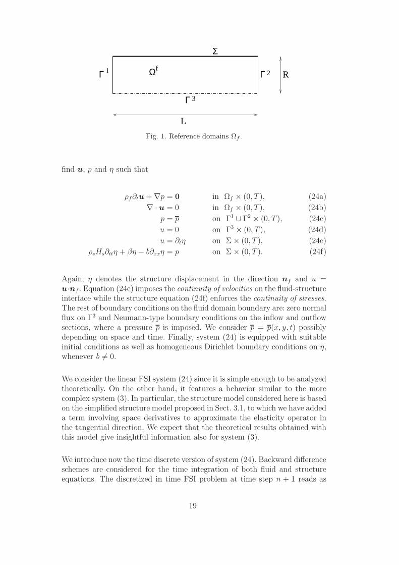
Fig. 1. Reference domains Ωf .

find u, p and η such that

ρf∂tu + ∇p = 0 in Ωf × (0, T ), (24a)

∇ · u = 0 in Ωf × (0, T ), (24b)

p = p on Γ1 ∪ Γ2 × (0, T ), (24c)

u = 0 on Γ3 × (0, T ), (24d)

u = ∂tη on Σ × (0, T ), (24e)

ρsHs∂ttη + βη − b∂xxη = p on Σ × (0, T ). (24f)

Again, η denotes the structure displacement in the direction nf and u =u·nf . Equation (24e) imposes the continuity of velocities on the fluid-structureinterface while the structure equation (24f) enforces the continuity of stresses.The rest of boundary conditions on the fluid domain boundary are: zero normalflux on Γ3 and Neumann-type boundary conditions on the inflow and outflowsections, where a pressure p is imposed. We consider p = p(x, y, t) possiblydepending on space and time. Finally, system (24) is equipped with suitableinitial conditions as well as homogeneous Dirichlet boundary conditions on η,whenever b 6= 0.

We consider the linear FSI system (24) since it is simple enough to be analyzedtheoretically. On the other hand, it features a behavior similar to the morecomplex system (3). In particular, the structure model considered here is basedon the simplified structure model proposed in Sect. 3.1, to which we have addeda term involving space derivatives to approximate the elasticity operator inthe tangential direction. We expect that the theoretical results obtained withthis model give insightful information also for system (3).

We introduce now the time discrete version of system (24). Backward differenceschemes are considered for the time integration of both fluid and structureequations. The discretized in time FSI problem at time step n + 1 reads as

19

follows: given ηn and un, find ηn+1, un+1 and pn+1 such that

ρfδtun+1 + ∇pn+1 = 0 in Ωf , (25a)

∇ · un+1 = 0 in Ωf , (25b)

pn+1 = pn+1 on Γ1 ∪ Γ2, (25c)

un+1 = 0 on Γ3, (25d)

un+1 = δtηn+1 on Σ, (25e)

ρsHsδttηn+1 + βηn+1 − b∂xxη

n+1 = pn+1 on Σ, (25f)

Assuming that the solution is regular enough, the fluid problem (25a)-(25e)can be reformulated only in terms of the pressure, obtaining the followingPoisson problem:

−∆pn+1 = 0 in Ωf , (26a)

pn+1 = pn+1 on Γ1 ∪ Γ2, (26b)

∂pn+1

∂n= 0 on Γ3, (26c)

∂pn+1

∂n= −ρfδtu

n+1 on Σ. (26d)

Let us introduce the solution pn+1 of the problem

−∆pn+1 = 0 in Ωf , (27a)

pn+1 = pn+1 on Γ1 ∪ Γ2, (27b)

∂pn+1

∂n= 0 on Γ3, (27c)

∂pn+1

∂n= 0 on Σ, (27d)

and the added-mass operator

M : H−1/2(Σ) → H1/2(Σ)

γ 7→ q|Σ,

which consists of: given γ ∈ H−1/2(Σ), find q ∈ H1(Ωf ) such that

−∆q = 0 in Ωf , (28a)

q = 0 on Γ1 ∪ Γ2, (28b)

∂q

∂n= 0 on Γ3, (28c)

∂q

∂n= γ on Σ. (28d)

and extract the value of the solution q on Σ. It can be proved that M(·) isa self-adjoint operator on L2(Σ) (see [3]). Then, the pressure pn+1 solution of

20

(26) on the interface Σ is given by

pn+1 = pn+1 − ρfM(δtun+1) on Σ. (29)

This relation holds for any (un+1, pn+1) satisfying (25a)-(25d), independentlyof the type of boundary condition taken on Σ for the fluid problem. Therefore,(29) holds for all the partitioned algorithms considered in this section.

In what follows, we will consider the Dirichlet-Neumann, the Robin-Dirichletand the Robin-Neumann algorithms. We will show that all of them can bewritten as fixed point algorithms on the variable ηn+1. We will also investigatethe convergence rates of such algorithms according to the following definition:

Definition 1 Let ηn+1 be the exact solution of the monolithic problem (25)and ηn+1,k the k − th iterate of the fixed point algorithm corresponding toeither DN, RD or RN algorithm. Given a relaxation parameter ω, we definethe asymptotic converge factor σ(ω) as the smallest positive number for which

‖ηn+1,k+1 − ηn+1‖L2(Σ) ≤ σ(ω)‖ηn+1,k − ηn+1‖L2(Σ)

holds for any possible solution ηn+1.

From now on, for the sake of clarity, we omit the temporal index n + 1, thatwill be understood.

To analyze the fixed point algorithms we will decompose η on the L2 orthonor-

mal basisgi(x) =

√2L

sin( iπxL

)∞

i=1, that is

η =∞∑

i=1

ηigi. (30)

Observe that the functions gi are both eigenfunctions of the added-mass op-erator (see [3]) with corresponding eigenvalues

µi =L

iπ tanh( iπRL

), i = 1, . . . ,∞, (31)

and eigenfunctions of the Laplace operator L = −∂xx on Σ, with correspondingeigenvalues

λi =(iπ

L

)2

.

In particular, we point out that the values λi increase with i and λi → ∞when i→ ∞, whereas the values µi decrese with i and µi → 0 when i→ ∞.

As we will show, for all three algorithms, the Fourier coefficients ηi satisfy thefixed point equation

ηk+1i = (1 − ωγi)η

ki + f(p, ηn, ηn−1,un), i = 1, . . . ,∞, (32)

21

for a suitable f and γi > 0. Hence, the following resut that applies for a generalRichardson algorithm (see e.g. [17]) can be used:

Lemma 1 For those algorithms that can be written in form (32), we have:

(1) the algorithm converges for

0 < ω <2

supi γi;

(2) there exists an optimal choice

ωopt =2

supi γi + infi γi

such that

σopt = σ(ωopt) =supi γi − infi γi

supi γi + infi γi

is minimal.

5.1 The Robin-Dirichlet algorithm

We begin by analyzing the Robin-Dirichlet algorithm for the proposed sim-plified problem. A Robin boundary condition for the fluid problem on Σ canbe easily obtained applying ρsHsδt(·) to (25e) and substituting the result in(25f). Then, (25e) is replaced by:

−ρsHsδtu+ p = βη − b∂xxη on Σ,

which can be written equivalently as

(β∆t2 + ρsHs)δtu− p = −βηn + b∂xxη − β∆tun on Σ.

Observe that this condition is consistent with the general Robin condition(7)a with the choice αf = ρsHs/∆t + β∆t. At this point, we can define theRobin-Dirichlet algorithm supplemented with a relaxation technique. For timestep n + 1 and iteration k + 1 with k > 0, the method consists of: given ηn,un and ηk, find ηk+1, uk+1 and pk+1 such that,

1. Fluid problem (Robin boundary condition)

ρfδtuk+1 + ∇pk+1 = 0, in Ωf , (33a)

∇ · uk+1 = 0 in Ωf , (33b)

pk+1 = p on Γ1 ∪ Γ2, (33c)

uk+1 = 0 on Γ3, (33d)

(β∆t2 + ρsHs)δtuk+1 − pk+1 = −βηn + b∂xxη

k − β∆tun on Σ. (33e)

22

2. Structure problem (Dirichlet boundary condition)

ηk+1 = ∆tuk+1 + ηn on Σ. (33f)

3. Relaxation step

ηk+1 = ωηk+1 + (1 − ω)ηk. (33g)

The relaxation parameter ω might be necessary to guarantee convergence ofthe method. We observe that for this simple case the structural equation isnever explicitly solved. This is due to the fact that the structure problem isa d − 1-dimensional manifold coupled via a Dirichlet boundary condition tothe fluid. We point out that the algorithm given by (33) coincides with theRobin-based scheme proposed in [15]. In the next theorem we analyze theconvergence properties of system (33).

Theorem 1 The Robin-Dirichlet iterative algorithm (33) applied to the FSItest problem (25) never converges to the monolithic solution, when b 6= 0, forany choice of ω > 0. Indeed, we have ωopt = 0 and σopt = 1. On the otherhand, when b = 0, the algorithm converges in just one iteration.

Proof . Substituting (29) in (33e) and thanks to (33f), we obtain

−ρfM(δttηk+1) + p = (β∆t2 + ρsHs)δttη

k+1 − b∂xxηk + βηn + β∆tun.

Due to the orthogonality of the basis gj∞

j=0, by multiplying the latter equalityby gi and integrating over Σ, we obtain

(ρfµi + β∆t2 + ρsHs)δttηk+1i = −bλiη

ki + p− βηn

i − β∆tuni .

The previous equation together with (33g) leads to:

1

ω(ρsHs + ρfµi + β∆t2)ηk+1

i =(

1 − ω

ω(ρsHs + ρfµi + β∆t2) − bλi∆t

2)ηk

i + f(pi, ηni , η

n−1i , un

i ),

for a suitable f . We have then,

ηk+1i =

(1 − ω

(1 +

bλi∆t2

ρsHs + ρfµi + β∆t2

))ηk

i + f(pi, ηni , η

n−1i , un

i )

and therefore we obtain (32) with

γi = 1 +bλi∆t

2

ρsHs + ρfµi + β∆t2. (34)

23

By noticing that the function γi increases with i, we have, for b 6= 0,

infiγi = γmin = 1 +

bλmin∆t2

ρsHs + ρfµmax + β∆t2,

supiγi = 1 +

b supi λi∆t2

ρsHs + ρf infi µi + β∆t2= +∞.

Therefore owing to Lemma 1, we can state that the algorithm never converges.

Otherwise, if b = 0, that is for the independent rings model, from (34) weobtain γi ≡ 0 and therefore, from Lemma 1, ωopt = 1 and σopt = 0. Thismeans that in this case RD scheme converges in exactly 1 iteration. This isnot surprising, since for b = 0 the RD algorithm coincides with the monolithicproblem (see [15]).

Remark 2 When considering discrete versions of the operators M and L,for instance by means of a finite elements discretization, we expect the discreteeigenvalues λi, µi to behave as

λmax = C1h−2, µmin = C2h, (35)

where h is the space discretization parameter on Σ. Therefore, we expect that

γmin ≃ 1 +bλmin∆t2

ρsHs + ρf µmax + β∆t2,

γmax ≃ 1 +bλmax∆t

2

ρsHs + ρf µmin + β∆t2,

obtaining, from Lemma 1 and owing to (35), that convergence should be reachedfor

0 < ω .2(ρsHs + C2ρfh+ β∆t2)

ρsHs + C2ρfh+ β∆t2 + C1b∆t2h−2.

Moreover, the best convergence rate is

σopt ≃

C1b∆t2h−2

ρsHs+C2ρf h+β∆t2− λminb∆t2

ρsHs+µmaxρf+β∆t2

2 + C1b∆t2h−2

ρsHs+C2ρf h+β∆t2+ λminb∆t2

ρsHs+µmaxρf +β∆t2

and therefore σopt < 1, that is, in practical computations, convergence is alwayspossible. In particular, if we satisfy a “CFL-like” condition ∆t ≃ kh and takethe limit ∆t→ 0, we observe that

σopt ≃C1kb

2ρsHs + C1kb.

24

We expect, then, the convergence to be fast if C1b << ρsHs and slow when theelasticity term dominates over the inertial one. This result is expected since inthe RD algorithm we treat explicitly the elastic term and implicitly the inertialterm.

5.2 The Robin-Neumann algorithm

In this section we prove convergence results for the Robin-Neumann algorithm,the most promising of the partitioned procedures designed in this work. Theonly difference with respect to system (33) is in the structure step, which doesinvolve the solution of the structural equation. As we will prove below, thisfact has a dramatic impact on the convergence properties of the algorithm(with respect to the Robin-Dirichlet method). For time step n + 1 and itera-tion k + 1 with k > 0, the Robin-Neumann method consists of: given ηn, un

and ηk, find ηk+1, uk+1 and pk+1 such that,

1. Fluid problem (33a)-(33e) (Robin boundary condition)2. Structure problem (Neumann boundary condition)

ρsHsδttηk+1 + βηk+1 − b∂xxη

k+1 = pk+1 on Σ. (36)

3. Relaxation step (33g).

The next theorem is devoted to the stability properties of this method.

Theorem 2 The Robin-Neumann iterative algorithm (33a)-(33e), (36), (33g)applied to the FSI test problem (25) converges to the monolithic solution underthe following condition for the relaxation parameter:

0 < ω < 2. (37)

Moreover, the convergence rate for ω = 1 is given by

σ(1) =1

1 +(

β∆t2+ρsHs

ρf µi+ β∆t2+ρsHs

bλi∆t2+ (β∆t2+ρsHs)2

bρf µiλi∆t2

) , (38)

whereas the best convergence rate is characterized by

σopt =1

1 + 2(

β∆t2+ρsHs

ρf µi+ β∆t2+ρsHs

bλi∆t2+ (β∆t2+ρsHs)2

bρf µiλi∆t2

) (39)

for a suitable index i = argmin(1 + β∆t2+ρsHs

ρf µi

)(1 + β∆t2+ρsHs

bλi∆t2

).

25

Proof . This result can be proved following the same lines as in the previoustheorem. From (29), we know that

M−1(pk+1 − p) = −ρfδtuk+1.

Invoking this equality in (33e) we get

(β∆t2 + ρsHs

ρfM−1 + I

)pk+1 = −b∂xxη

k + f(p, ηn,un), (40)

for a suitable f and where I is the identity operator. On the other hand, thevalue of pk+1 is determined by (36):

pk+1 = ρsHsδttηk+1 + βηk+1 − b∂xxη

k+1. (41)

Combining (40) and (41), we obtain:

(β∆t2 + ρsHs

ρfM−1 + I

) (ρsHsδttη

k+1 + βηk+1 − b∂xxηk+1

)

= −b∂xxηk + f(p, ηn,un). (42)

As above, we can use the decomposition (30) and write the previous equationfor every component ηk+1

i . Let us define the following value:

ψi =(β∆t2 + ρsHs

ρfµi+ 1

) (ρsHs

∆t2+ β + bλi

).

It allows us to write (42) in form (32) with

γi = 1 −bλi

ψi.

We observe that 0 < γi ≤ 1 and it is not monotone in general. In particular,it reaches its maximum for i → ∞ (where γi → 1) and its minimum for asuitable index i depending on the parameters of the problem. Then, owing toLemma 1 and rearranging, we obtain (37) and (39). Moreover, if ω = 1, from(32) we obtain σ(1) = maxi |1 − γi| = 1 − γi, leading to (38).

Remark 3 When b = 0 the RN scheme coincides with the monolithic prob-lem. Indeed, from (39) it follows that ωopt = 1 and σopt = 0 and then RNconverges in just one iteration. On the other hand, when b 6= 0 and ∆t → 0,the convergence gets faster and faster.

From (39), we observe that the convergence rate gets worse if the ratio ρs/ρf

decreases or if the elastic term b increases. However, due to the presence ofthree terms in the bracket in (39), the value of σopt is in any case far from 1,and therefore it seems that the RN scheme is not too sensible to the variation

26

of b and to the added-mass effect, as the numerical results in Sect. 6 confirm.The same considerations holds when using ω = 1, since σ(1) exhibits the samedependence on the parameters.

5.3 The Dirichlet-Neumann algorithm

In this section, we extend the results shown in [3], concerning the convergenceof the DN algorithm, to the generalized string model. Moreover, we providealso for this scheme the optimal values of the asymptotic converge factor. Inparticular, we have the following

Theorem 3 The Dirichlet-Neumann iterative algorithm applied to the FSItest problem (25) converges to the monolithic solution under the followingcondition on the relaxation parameter:

0 < ω ≤2

1 +µmaxρf

ρsHs+β∆t2+λminb∆t2

. (43)

Moreover, the best convergence rate is characterized by

σopt =1

1 + 2ρsHs+β∆t2+bλmin∆t2

µmaxρf

. (44)

Proof . In this case we can write the algorithm in form (32) with

γi = 1 +ρfµi

ρsHs + β∆t2 + b∆t2λi.

By noticing that the function γi decreases with i, owing to Lemma 1 we obtain(43) and (44).

From (44), we observe that the convergence rate gets worse if b decreases.Moreover, it depends heavily on the ratio ρs/ρf , that is the DN scheme isvery sensible to the added-mass effect, as already pointed out in [3] and as thenumerical results confirm.

6 Numerical results

In this section we present some numerical results with the aim of testing thealgorithms proposed in the previous sections. As pointed out in Section 2.1,we call semi-implicit the algorithms in which we do not update in the loopneither the convective term nor the fluid domain, otherwise we refer to them

27

as implicit. In particular, in Section 6.1 we test the performance of the semi-implicit Robin-Dirichlet (ERD) and Robin-Neumann (ERN) algorithms, incomparison with the semi-implicit Dirichlet-Neumann scheme (EDN). More-over, we test the implicit Robin-Neumann algorithm (IRN). In Section 6.2 wedetail the performance of the semi-implicit Robin-Robin, Dirichlet-Robin andNeumann-Robin algorithms.

For the structure, we consider the following equation of linear elasticity

ρs∂ttη − c∇ · (∇η + (∇η)t) − λ∇ · ((∇ · η)I) + βη = f s,

where I is the identity operator, c = E/(1+ ν), λ = νE/((1+ ν)(1−2ν)) andβ = E/(1− ν2)R2, where E is the Young modulus, ν the Poisson ratio and Rthe radius of the fluid domain. The reaction terms stand for the transversalmembrane effects that appear when the structure is written in axisymmetricform.

All the numerical simulations are performed in a rectangular domain both forthe fluid and for the two structures, whose size is 6 × 1 cm and 6 × 0.1 cm,respectively (see Fig. 2). We use a 2D Finite Element Code written in Matlab

Ω

Ω

Ω

f0

0s

s0

Fig. 2. Computational fluid and structure domains.

at MOX - Dipartimento di Matematica - Politecnico di Milano and at CMCS -EPFL - Lausanne. Moreover, we consider P1isoP2 and P1 elements for the fluidand P1 element for the structure and a space discretization step h = 0.02 cm.In all the cases we use the residual normalized on the initial one as stoppingcriterion (see Sect. 4), with a tolerance equal to 10−4.

We set µ = 0.035 cm2/s and ρf = 1 g/cm2 and, unless otherwise specified, weconsider the following other values: ∆t = 10−3s, ρs = 1.1 g/cm2, c = 1.15 ·106 dyne, λ = 1.7 ·106 dyne, β = 4 ·106 dyne/cm2 (corresponding to the valuesE = 0.158MPa and ν = 0.37) and the thickness of the structure Hs = 0.1 cm.

6.1 The Robin-Neumann and the Robin-Dirichlet schemes

In this section we study the performance of the Robin-Neumann and theRobin-Dirichlet schemes. When we prescribe a Robin boundary condition

28

for the fluid, an optimal choice for the parameter αf , as (12) suggests, isnaturally given by the simplified model for the structure equation, that isαf = Hsρs/∆t+ β∆t. This value is directly computable, hence very useful inpractical computations.

Let us start with the semi-implicit case. In Fig. 3 we show the solution com-puted with the ERN scheme, which, of course, is the same as the one computedwith the semi-implicit monolithic scheme (EM), up to the employed tolerance.In particular, this figure shows average quantities on a radial section of themean pressure (top), the flow rate (middle), and the fluid domain radius (bot-tom), as a function of the axial coordinate.

0 2 4 6

0

2000

4000

6000

8000

10000

axial coordinate [cm]

mean

pres

sure

[dyne

/cm2 ]

0 2 4 6

0

2000

4000

6000

8000

axial coordinate [cm]

mean

pres

sure

[dyne

/cm2 ]

0 2 4 6

0

1000

2000

3000

4000

5000

axial coordinate [cm]

mean

pres

sure

[dyne

/cm2 ]

0 2 4 6

0

5

10

15

20

25

axial coordinate [cm]

flow

rate [

cm2 /s]

0 2 4 6

0

5

10

15

axial coordinate [cm]

flow

rate [

cm2 /s]

0 2 4 6

0

5

10

15

axial coordinate [cm]

flow

rate [

cm2 /s]

0 2 4 6

1

1.01

1.02

1.03

1.04

1.05

1.06

axial coordinate [cm]

fluid

doma

in rad

ius [c

m]

0 2 4 61

1.01

1.02

1.03

axial coordinate [cm]

fluid

doma

in rad

ius [c

m]

0 2 4 6

1

1.005

1.01

1.015

1.02

1.025

axial coordinate [cm]

fluid

doma

in rad

ius [c

m]

t = 0.004 s, t = 0.008 s, t = 0.012 s

Fig. 3. ERN scheme. Mean pressure (top), flow rate (middle) and fluid domainradius (bottom) at three time instants.

Fig. 4 shows the structure displacement, obtained with the ERN scheme, inthe deformed domain at three different instants. In Tab. 2 we show the av-

0 1 2 3 4 5 6

0.5

0.52

0.54

0.56

0.58

0.6

0.62

0.64

0.66

0.68

0.7

0

0.01

0.02

0 1 2 3 4 5 6

0.5

0.52

0.54

0.56

0.58

0.6

0.62

0.64

0.66

0.68

0.7

5

10

15

x 10−3

0 1 2 3 4 5 6

0.5

0.52

0.54

0.56

0.58

0.6

0.62

0.64

0.66

0.68

0.7

0

5

10

x 10−3

Fig. 4. Displacement of the structure - ERN scheme - t = 0.004 s (left), t = 0.008 s(middle) and at t = 0.012 s (right).

erage number of iterations in the first 12 time steps, employed by the ERN,ERD and EDN schemes, in three cases: without relaxation (ω = 1), with anoptimally tuned relaxation parameter (ωopt) and using an Aitken relaxationprocedure (see [4]). First of all, we point out that ERN is the only algorithmthat converges without relaxation. This is a very interesting feature of thisscheme. Moreover, ERN is always much faster than EDN. This is confirmed

29

also by Fig. 5 that plots the errors on several quantities, measured in the L∞

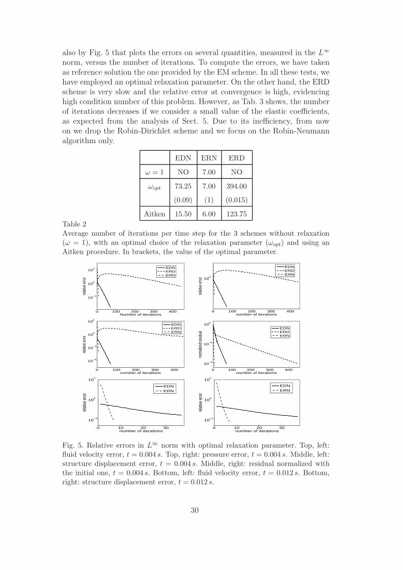
norm, versus the number of iterations. To compute the errors, we have takenas reference solution the one provided by the EM scheme. In all these tests, wehave employed an optimal relaxation parameter. On the other hand, the ERDscheme is very slow and the relative error at convergence is high, evidencinghigh condition number of this problem. However, as Tab. 3 shows, the numberof iterations decreases if we consider a small value of the elastic coefficients,as expected from the analysis of Sect. 5. Due to its inefficiency, from nowon we drop the Robin-Dirichlet scheme and we focus on the Robin-Neumannalgorithm only.

EDN ERN ERD

ω = 1 NO 7.00 NO

ωopt 73.25 7.00 394.00

(0.09) (1) (0.015)

Aitken 15.50 6.00 123.75

Table 2Average number of iterations per time step for the 3 schemes without relaxation(ω = 1), with an optimal choice of the relaxation parameter (ωopt) and using anAitken procedure. In brackets, the value of the optimal parameter.

0 100 200 300 400

10−2

100

102

Number of iterations

relat

ive er

ror

EDNERDERN

0 100 200 300 400

100

number of iterations

relat

ive e

rror

EDNERDERN

0 100 200 300 400

10−4

10−2

100

102

number of iterations

relat

ive er

ror

EDNERDERN

0 100 200 300 400

10−4

10−2

100

number of iterations

norm

alize

d res

idual

EDNERDERN

0 10 20 30

10−2

100

102

number of iterations

relat

ive er

ror

EDNERN

0 10 20 30

10−2

100

102

number of iterations

relat

ive er

ror

EDNERN

Fig. 5. Relative errors in L∞ norm with optimal relaxation parameter. Top, left:fluid velocity error, t = 0.004 s. Top, right: pressure error, t = 0.004 s. Middle, left:structure displacement error, t = 0.004 s. Middle, right: residual normalized withthe initial one, t = 0.004 s. Bottom, left: fluid velocity error, t = 0.012 s. Bottom,right: structure displacement error, t = 0.012 s.

30

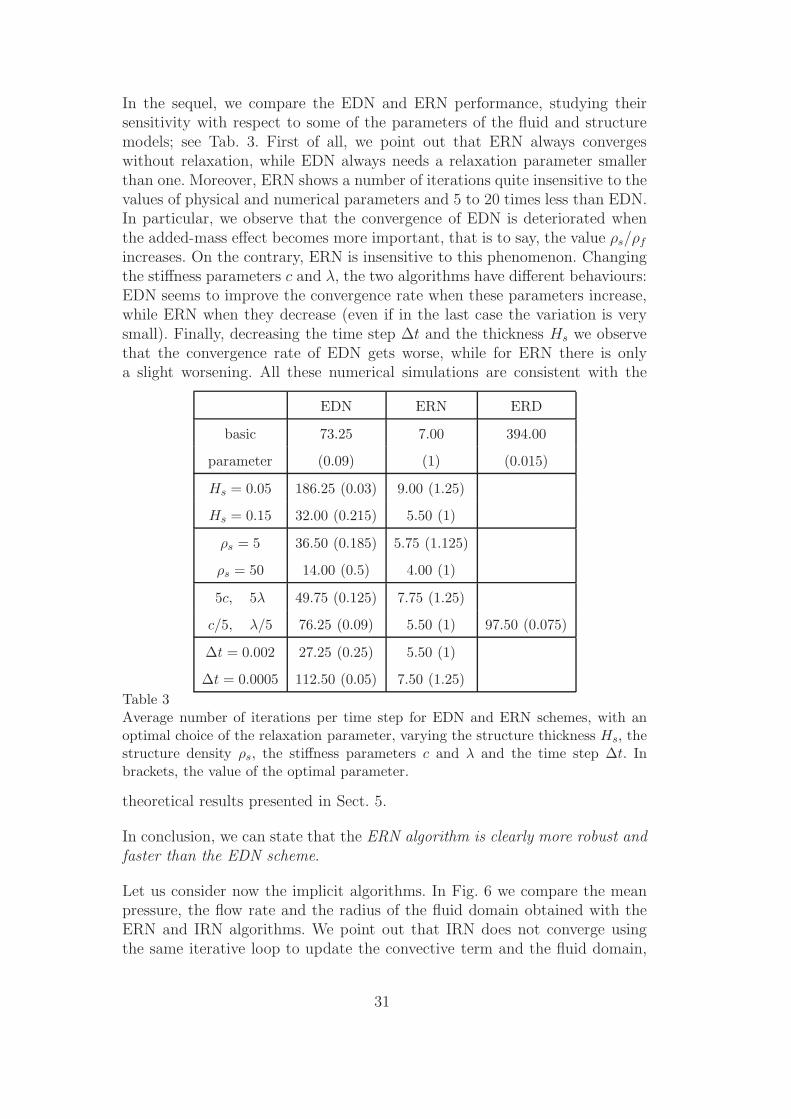
In the sequel, we compare the EDN and ERN performance, studying theirsensitivity with respect to some of the parameters of the fluid and structuremodels; see Tab. 3. First of all, we point out that ERN always convergeswithout relaxation, while EDN always needs a relaxation parameter smallerthan one. Moreover, ERN shows a number of iterations quite insensitive to thevalues of physical and numerical parameters and 5 to 20 times less than EDN.In particular, we observe that the convergence of EDN is deteriorated whenthe added-mass effect becomes more important, that is to say, the value ρs/ρf

increases. On the contrary, ERN is insensitive to this phenomenon. Changingthe stiffness parameters c and λ, the two algorithms have different behaviours:EDN seems to improve the convergence rate when these parameters increase,while ERN when they decrease (even if in the last case the variation is verysmall). Finally, decreasing the time step ∆t and the thickness Hs we observethat the convergence rate of EDN gets worse, while for ERN there is onlya slight worsening. All these numerical simulations are consistent with the

EDN ERN ERD

basic 73.25 7.00 394.00

parameter (0.09) (1) (0.015)

Hs = 0.05 186.25 (0.03) 9.00 (1.25)

Hs = 0.15 32.00 (0.215) 5.50 (1)

ρs = 5 36.50 (0.185) 5.75 (1.125)

ρs = 50 14.00 (0.5) 4.00 (1)

5c, 5λ 49.75 (0.125) 7.75 (1.25)

c/5, λ/5 76.25 (0.09) 5.50 (1) 97.50 (0.075)

∆t = 0.002 27.25 (0.25) 5.50 (1)

∆t = 0.0005 112.50 (0.05) 7.50 (1.25)

Table 3Average number of iterations per time step for EDN and ERN schemes, with anoptimal choice of the relaxation parameter, varying the structure thickness Hs, thestructure density ρs, the stiffness parameters c and λ and the time step ∆t. Inbrackets, the value of the optimal parameter.

theoretical results presented in Sect. 5.

In conclusion, we can state that the ERN algorithm is clearly more robust andfaster than the EDN scheme.

Let us consider now the implicit algorithms. In Fig. 6 we compare the meanpressure, the flow rate and the radius of the fluid domain obtained with theERN and IRN algorithms. We point out that IRN does not converge usingthe same iterative loop to update the convective term and the fluid domain,

31

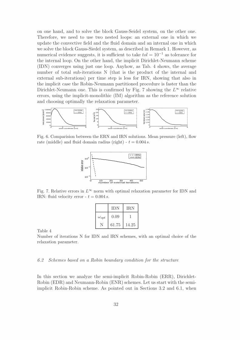
on one hand, and to solve the block Gauss-Seidel system, on the other one.Therefore, we need to use two nested loops: an external one in which weupdate the convective field and the fluid domain and an internal one in whichwe solve the block Gauss-Siedel system, as described in Remark 1. However, asnumerical evidence suggests, it is sufficient to take tol = 10−1 as tolerance forthe internal loop. On the other hand, the implicit Dirichlet-Neumann scheme(IDN) converges using just one loop. Anyhow, as Tab. 4 shows, the averagenumber of total sub-iterations N (that is the product of the internal andexternal sub-iterations) per time step is less for IRN, showing that also inthe implicit case the Robin-Neumann partitioned procedure is faster than theDirichlet-Neumann one. This is confirmed by Fig. 7 showing the L∞ relativeerrors, using the implicit-monolithic (IM) algorithm as the reference solutionand choosing optimally the relaxation parameter.

0 2 4 60

2000

4000

6000

8000

10000

axial coordinate [cm]

mean

pres

sure

[dyne

/cm2 ]

ERNIRN

0 2 4 6

0

5

10

15

20

25

axial coordinate [cm]

flow

rate [

cm2 /s]

ERNIRN

0 2 4 6

1

1.01

1.02

1.03

1.04

1.05

1.06

axial coordinate [cm]

fluid

doma

in ra

dius [

cm]

ERNIRN

Fig. 6. Comparision between the ERN and IRN solutions. Mean pressure (left), flowrate (middle) and fluid domain radius (right) - t = 0.004 s.

0 10 20 30 40 50

10−4

10−2

100

number of external iterations

relati

ve er

ror

IRNIDN

Fig. 7. Relative errors in L∞ norm with optimal relaxation parameter for IDN andIRN: fluid velocity error - t = 0.004 s.

IDN IRN

ωopt 0.09 1

N 61.75 14.25

Table 4Number of iterations N for IDN and IRN schemes, with an optimal choice of therelaxation parameter.

6.2 Schemes based on a Robin boundary condition for the structure

In this section we analyze the semi-implicit Robin-Robin (ERR), Dirichlet-Robin (EDR) and Neumann-Robin (ENR) schemes. Let us start with the semi-implicit Robin-Robin scheme. As pointed out in Sections 3.2 and 6.1, when

32

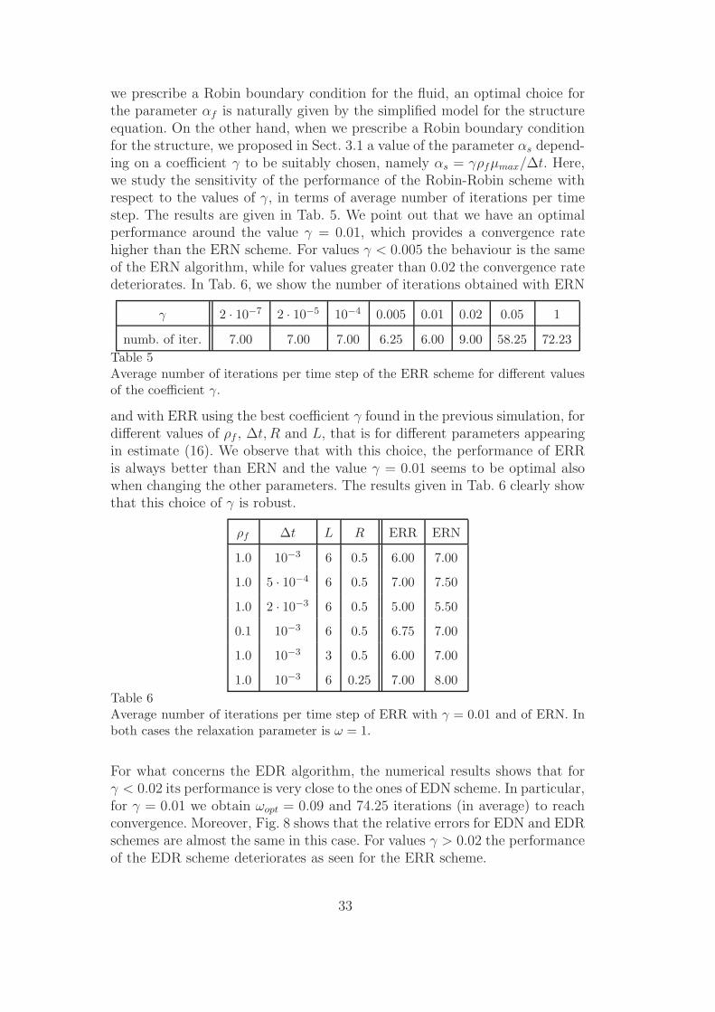
we prescribe a Robin boundary condition for the fluid, an optimal choice forthe parameter αf is naturally given by the simplified model for the structureequation. On the other hand, when we prescribe a Robin boundary conditionfor the structure, we proposed in Sect. 3.1 a value of the parameter αs depend-ing on a coefficient γ to be suitably chosen, namely αs = γρfµmax/∆t. Here,we study the sensitivity of the performance of the Robin-Robin scheme withrespect to the values of γ, in terms of average number of iterations per timestep. The results are given in Tab. 5. We point out that we have an optimalperformance around the value γ = 0.01, which provides a convergence ratehigher than the ERN scheme. For values γ < 0.005 the behaviour is the sameof the ERN algorithm, while for values greater than 0.02 the convergence ratedeteriorates. In Tab. 6, we show the number of iterations obtained with ERN

γ 2 · 10−7 2 · 10−5 10−4 0.005 0.01 0.02 0.05 1

numb. of iter. 7.00 7.00 7.00 6.25 6.00 9.00 58.25 72.23

Table 5Average number of iterations per time step of the ERR scheme for different valuesof the coefficient γ.

and with ERR using the best coefficient γ found in the previous simulation, fordifferent values of ρf , ∆t, R and L, that is for different parameters appearingin estimate (16). We observe that with this choice, the performance of ERRis always better than ERN and the value γ = 0.01 seems to be optimal alsowhen changing the other parameters. The results given in Tab. 6 clearly showthat this choice of γ is robust.

ρf ∆t L R ERR ERN

1.0 10−3 6 0.5 6.00 7.00

1.0 5 · 10−4 6 0.5 7.00 7.50

1.0 2 · 10−3 6 0.5 5.00 5.50

0.1 10−3 6 0.5 6.75 7.00

1.0 10−3 3 0.5 6.00 7.00

1.0 10−3 6 0.25 7.00 8.00

Table 6Average number of iterations per time step of ERR with γ = 0.01 and of ERN. Inboth cases the relaxation parameter is ω = 1.

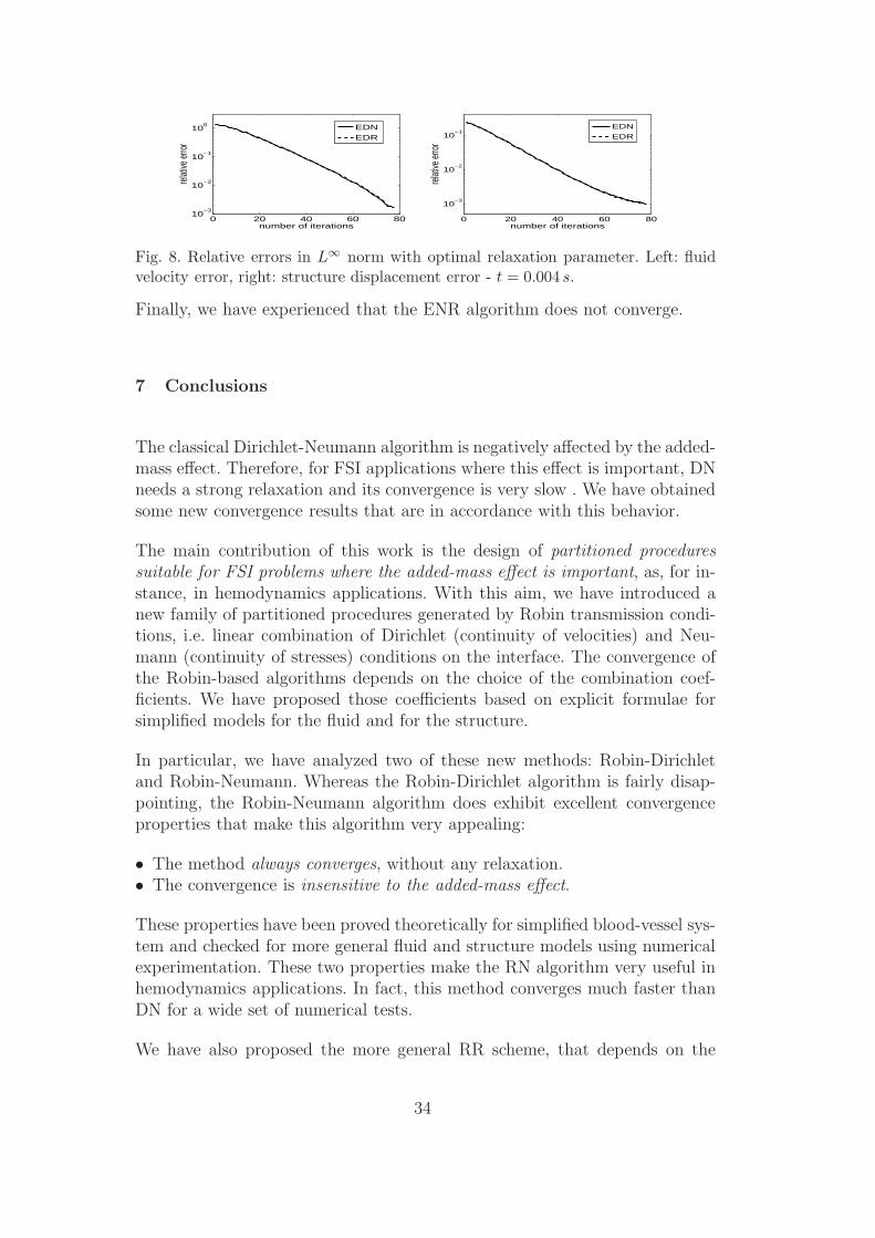
For what concerns the EDR algorithm, the numerical results shows that forγ < 0.02 its performance is very close to the ones of EDN scheme. In particular,for γ = 0.01 we obtain ωopt = 0.09 and 74.25 iterations (in average) to reachconvergence. Moreover, Fig. 8 shows that the relative errors for EDN and EDRschemes are almost the same in this case. For values γ > 0.02 the performanceof the EDR scheme deteriorates as seen for the ERR scheme.

33

0 20 40 60 8010

−3

10−2

10−1

100

number of iterations

relat

ive er

ror

EDNEDR

0 20 40 60 80

10−3

10−2

10−1

number of iterations

relat

ive er

ror

EDN

EDR

Fig. 8. Relative errors in L∞ norm with optimal relaxation parameter. Left: fluidvelocity error, right: structure displacement error - t = 0.004 s.

Finally, we have experienced that the ENR algorithm does not converge.

7 Conclusions

The classical Dirichlet-Neumann algorithm is negatively affected by the added-mass effect. Therefore, for FSI applications where this effect is important, DNneeds a strong relaxation and its convergence is very slow . We have obtainedsome new convergence results that are in accordance with this behavior.

The main contribution of this work is the design of partitioned proceduressuitable for FSI problems where the added-mass effect is important, as, for in-stance, in hemodynamics applications. With this aim, we have introduced anew family of partitioned procedures generated by Robin transmission condi-tions, i.e. linear combination of Dirichlet (continuity of velocities) and Neu-mann (continuity of stresses) conditions on the interface. The convergence ofthe Robin-based algorithms depends on the choice of the combination coef-ficients. We have proposed those coefficients based on explicit formulae forsimplified models for the fluid and for the structure.

In particular, we have analyzed two of these new methods: Robin-Dirichletand Robin-Neumann. Whereas the Robin-Dirichlet algorithm is fairly disap-pointing, the Robin-Neumann algorithm does exhibit excellent convergenceproperties that make this algorithm very appealing:

• The method always converges, without any relaxation.• The convergence is insensitive to the added-mass effect.

These properties have been proved theoretically for simplified blood-vessel sys-tem and checked for more general fluid and structure models using numericalexperimentation. These two properties make the RN algorithm very useful inhemodynamics applications. In fact, this method converges much faster thanDN for a wide set of numerical tests.

We have also proposed the more general RR scheme, that depends on the

34

scaling factor γ. By suitably tuning this coefficient, we obtain convergenceproperties for the RR scheme even better than those of the RN algorithm.Moreover, the tuned value seems to be very robust and pratically independentof some of the parameters defining the problem at hand.

Even though we have not considered this point in this article, the use of aRobin transmission condition for the fluid system allows to solve FSI prob-lems with enclosed fluid domains (balloon-type problems). The DN algorithmis useless in these cases because the fluid sub-problem is confined (Dirich-let boundary conditions on the whole fluid boundary). Furthermore, thoseDirichlet boundary conditions for the fluid are obtained from the structuresub-problem and do not satisfy

∫

∂Ωf

u · nf = 0

in general. Thus, the null divergence constraint cannot be fulfilled, leading tounphysical results. The application of RN to this kind of problems will be thesubject of a future work.

Acknowledgments

The authors gratefully acknowledge Annalisa Quaini for her suggestions. Thefirst author acknowledges the support of the European Community throughthe Marie Curie contract NanoSim (MOIF-CT-2006-039522). The second andthird authors acknowledge the Italian grant PRIN 2005 “Numerical Model-ing for Scientific Computing and Advanced Applications”. The third authoralso acknowledges the support of Fondazione Cariplo, Milan, Italy, under theproject “Modellistica Matematica di Materiali Microstrutturati per Disposi-tivi a Rilascio di Farmaco”.

References

[1] S. Badia, A. Quaini, and A. Quarteroni. Splitting methods based onalgebraic factorization for fluid-structure interaction. MOX Report n. 03/2007,Submitted.

[2] K. J. Bathe, H. Zhang, and M.H. Wang. Finite element analysis ofincompressible and compressible fluid flows with free surfaces and structuralinteractions. Comp. Struct., 56:193–213, 1995.

[3] P. Causin, J.F. Gerbeau, and F. Nobile. Added-mass effect in the designof partitioned algorithms for fluid-structure problems. Computer Methods inApplied Mechanics and Engineering, 194(42-44):4506–4527, 2005.

35

[4] S. Deparis. Numerical analysis of axisymmetric flows and methods for fluid-structure interaction arising in blood flow simulation. PhD thesis, EcolePolytechnique Federale de Lausanne, 2004.

[5] S. Deparis, M. Discacciati, G. Fourestey, and A. Quarteroni. Fluid-structurealgorithms based on Steklov-Poincare operators. Computer Methods in AppliedMechanics and Engineering, 195(41-43):5797–5812, 2006.

[6] J. Donea. An arbitrary Lagrangian-Eulerian finite element method for transientdynamic fluid-structure interaction. Computer Methods in Applied Mechanicsand Engineering, 33:689–723, 1982.

[7] M.A. Fernandez, J.F. Gerbeau, and C. Grandmont. A projection semi-implicitscheme for the coupling of an elastic structure with an incompressible fluid.International Journal for Numerical Methods in Engineering, 69(4):794–821,2007.

[8] M.A. Fernandez and M. Moubachir. A Newton method using exact Jacobiansfor solving fluid-structure coupling. Computers & Structures, 83(2-3):127–142,2005.

[9] C. Forster, W. Wall, and E. Ramm. Artificial added mass instabilities insequential staggered coupling of nonlinear structures and incompressible viscousflow. Computer Methods in Applied Mechanics and Engineering, 196(7):1278–1293, 2007.

[10] J. F. Gerbeau and M. Vidrascu. A quasi-newton algorithm based on a reducedmodel for fluid-structure interactions problems in blood flows. Math. Model.Num. Anal., 37(4):631–648, 2003.

[11] T. J. R. Hughes, W. K. Liu, and T. K. Zimmermann. Lagrangian-Eulerianfinite element formulation for incompressible viscous flows. Computer Methodsin Applied Mechanics and Engineering, 29(3):329–349, 1981.

[12] P. Le Tallec and J. Mouro. Fluid structure interaction with large structuraldisplacements. Computer Methods in Applied Mechanics and Engineering,190:3039–3067, 2001.

[13] H.G. Matthies and J. Steindorf. Partitioned but strongly coupled iterationschemes for nonlinear fluid-structure interaction. Computers & Structures,80:1991–1999, 2002.

[14] F. Nobile. Numerical Approximation of Fluid-Structure Interaction problemswith application to Haemodynamics. PhD thesis, Ecole Polytechnique Federalede Lausanne, 2001.

[15] F. Nobile and C. Vergara. An effective fluid-structure interaction formulationfor vascular dynamics by generalized robin conditions. MOX Report n. 01/2007,Accepted for pubblication on SIAM J. Sc. Comp.

[16] S. Piperno and C. Farhat. Design of efficient partitioned procedures for transientsolution of aerolastic problems. Rev. Eur. Elements Finis, 9(6-7):655–680, 2000.

36

[17] A. Quarteroni, R. Sacco, and F. Saleri. Numerical mathematics. Springer Berlin,2000.

[18] A. Quarteroni, M. Tuveri, and A. Veneziani. Computational vascular fluiddynamics: Problems, models and methods. Computing and Visualisation inScience, 2:163–197, 2000.

37