fluids 2 lecture 2 - wordpress.com · • no tutorial week 3 ‐3rd october 2013 –this thursday....

ENG2038M – Fluid Mechanics 2

Lecture 2Flow classifications and continuity

Dr Tim Gough: [email protected]


General information 1

• Laboratory classes – these are still being allocated.

• For those allocated in group 2J1 (Civil Eng.) the week 4 laboratory is postponed (tutor in Belfast). Please watch your email.

• No tutorial week 3 ‐ 3rd October 2013 – this Thursday. Attempt tutorial based on examples from today’s lecture.

• As per usual, any problems email [email protected]

• On email while here:

www.esrf.eu


• Is Blackboard working yet?

• Currently 137 students registered on e‐vision.

• If yes, good. If no, then continue to use http://skeddanblog.wordpress.com/

• Please also continue to watch email for announcements.

• Questions?

General information 2


Lecture 1 recap

Elastic solids Newtonian fluids

Dynamic viscosity Kinematic viscosity


Lecture 1 recap

Bernoulli• Ps is static pressure = gh

• is dynamic pressure

Reynolds number is the ratio of inertial to viscous forces in a flow

where: is density in kg/m3

V is velocity in m/sL is a length in m is viscosity in Pa.s


If Re < 2000 the flow is laminar

If 2000 < Re < 4000 the flow is transitional

If Re > 4000 the flow is turbulent• For pipe flow only!

Lecture 1 recap


Fluid Flow


Fluid flow

• The motion of a fluid is usually extremely complex.

• Studies of fluids at rest, or in equilibrium, are simplified by the absence of shear forces within the fluid.

• When a fluid flows over a surface or other boundary, whether at rest or in motion, the velocity of the fluid in contact with the boundary must be the same as that of the boundary and a velocity gradient is created at right angles to the boundary.


Fluid flow

• The resulting change of velocity from layer to layer of fluid flowing parallel to the boundary gives rise to shear stresses in the fluid.

• If an individual particle of fluid is coloured, or otherwise rendered visible, it will describe a pathline.

• A pathline is the trace showing the position of the particle at successive intervals of time from a given point.

• If instead of colouring an individual particle, the flow pattern is made visible by injecting a stream of dye (liquid) or smoke (gas) the result will be a streakline (or filament line) which gives an instantaneous picture of the positions of all particles that have passed through the point at which the dye (or smoke) was injected.

• Since the flow may change with time a pathline and a streaklineneed not be the same.


Fluid flow• When choosing a dye or other tracer it is clearly very important to

match the density and other physical properties as closely as possible to the carrier fluid (isokinetic).

• Streamlines are curves that are everywhere tangential to the velocity vector.


Streaklines


Streaklines

Flow around an aerofoil – very low velocity


Uniform and steady flows


Uniform and steady flows

• Conditions in a body of fluid can vary from point to point and, at any given point, can vary from one moment of time to the next.

• Flow is described as uniform if the velocity at a given instant is the same in magnitude and direction at every point in the fluid.

• If, at a given instant, the velocity changes from point to point, the flow is described as non‐uniform.

• A steady flow is one in which the velocity, pressure and cross‐section of the stream may vary from point to point but do not vary with time.

• If, at any given point, conditions do change with time, the flow is described as unsteady.


Four possible types of flow1. Steady uniform flow

Conditions do not change with position or time. The velocity and cross sectional area of the stream of fluid are the same at each cross section.

Pipe flow – could be laminar or turbulent


2. Steady non‐uniform flow

Conditions change from point to point but not with time. The velocity and cross‐sectional area of the stream may vary from cross‐section to cross‐section but, for each cross‐section, they will not vary with time.

Four possible types of flow

Flow through tapering pipe


Four possible types of flow3. Unsteady uniform flow

At a given instant of time the velocity at every point is the same, but the velocity will change with time.

Start up flow of molten LDPE


Four possible types of flow4. Unsteady non‐uniform flow

The cross‐sectional area and velocity vary from point to point and also change with time.

Wave travelling along a channel


Viscous and inviscid flows



• When a real fluid flows past a boundary, the fluid immediately in contact with the boundary will have the same velocity as the boundary.

• Further away from the boundary (or wall) perpendicularly the effects of the boundary diminish.

• Eventually the effects of the boundary become negligible.

• Since the effects of the boundary are due to the viscosity of the fluid, the flow near to the boundary is known as a viscous flow.

• Well away from the boundary the flow can be treated as being inviscid(or non‐viscous).

• The region near to the boundary is known as the boundary layer –about which more later.



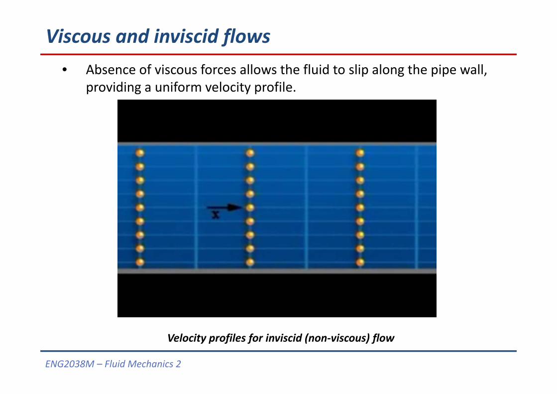
Velocity profiles for inviscid (non‐viscous) flow

• Absence of viscous forces allows the fluid to slip along the pipe wall, providing a uniform velocity profile.



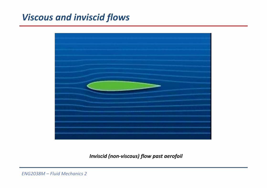
Inviscid (non‐viscous) flow past aerofoil


Viscous and inviscid flows• With viscosity involved, if the velocity at the wall is zero (no‐slip) then

we must have a velocity profile near the wall.

Velocity profiles for viscous flow


Viscous flow over flat plate

The flow away from the walls can be treated as inviscid.But near the walls the viscosity is important.


Viscous flow over flat plate

• The region where viscous effects dominate is called the boundary layer (about which more later).


Boundary layers over a flat plate

ENG2038M – Fluid Mechanics 2ENG2038M – Fluid Mechanics 2

Discharge and mean velocity



• The total quantity of fluid flowing in time past any particular cross‐section of a stream is called the discharge or flow at that section.

• It can be expressed either in terms of:

• Mass flowrate (kg/s) or

• Volumetric flowrate, Q (m3/s)

• Clearly we can move between the two flowrates, for an incompressible fluid using the simple relation:


b) Turbulent flow

VVr

a) Laminar flow

Discharge and mean velocity• In an ideal fluid, where there is no friction, the velocity, V, would be

the same at every point across the cross section.

• If the cross section has an area A then we can say that the volume passing would be V x A, i.e.

• In a real fluid however the velocity at the wall is the same as that of the wall (see the no‐slip condition later)

rr

R



• If V is the velocity at any radius r, the flow Q through an annular element of radius r and thickness r will be:

2

Hence:

/

In many problems we simply assume a constant velocity equal to the mean velocity to give:

b) Turbulent flow

Vrr

R

Vr

a) Laminar flow


Continuity of flow


Continuity of flow

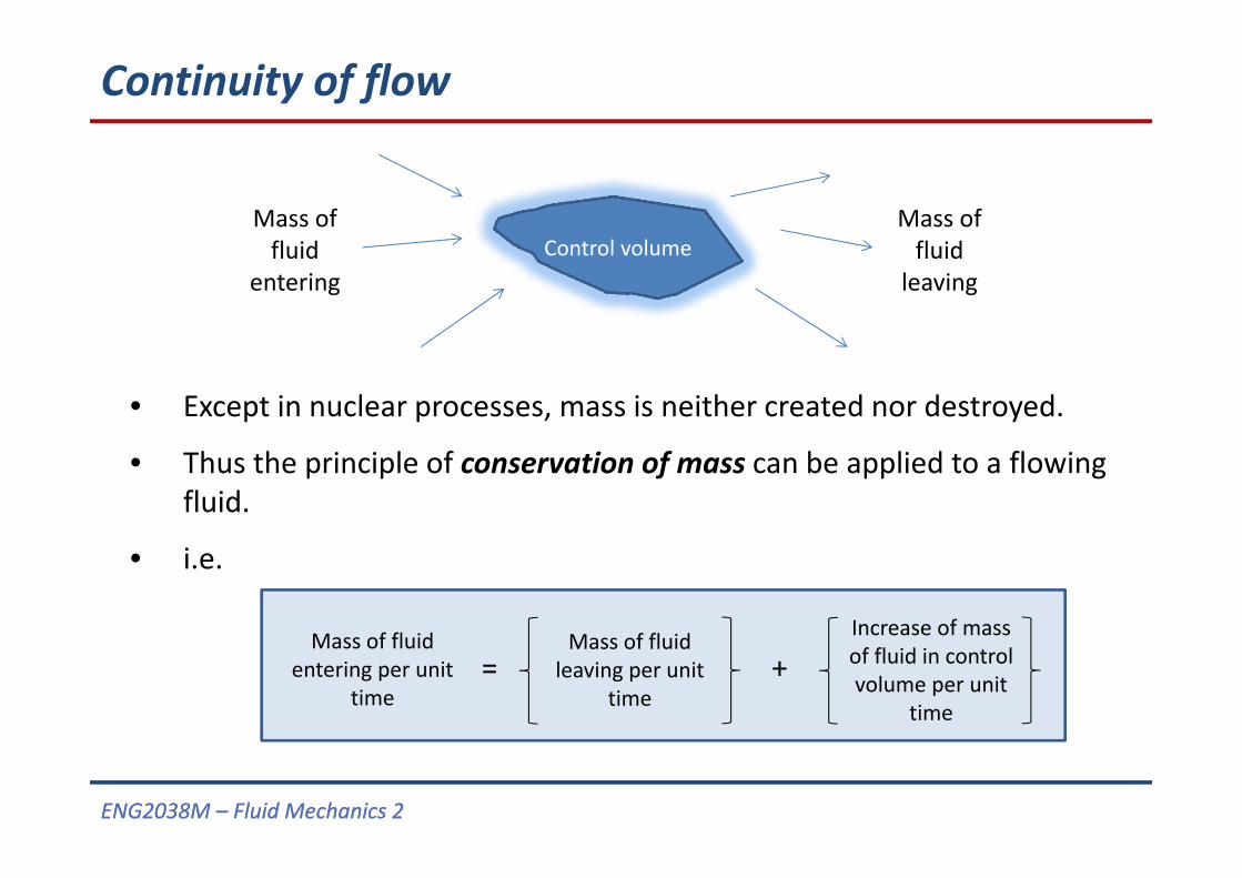
Control volumeMass of fluid

entering

Mass of fluid

leaving

• Except in nuclear processes, mass is neither created nor destroyed.

• Thus the principle of conservation of mass can be applied to a flowing fluid.

• i.e.

Mass of fluid entering per unit

time=

Mass of fluid leaving per unit

time+

Increase of mass of fluid in control volume per unit

time


Continuity of flow• For steady flow we can write:

Mass of fluid entering per unit

time=

Mass of fluid leaving per unit

time

12

Area = A1Velocity = V1Density = 1

Area = A2Velocity = V2Density = 2

• For a streamtube (no fluid crosses boundary):


Continuity of flow

• This is the equation of continuity for the flow of a compressible fluid through a streamtube.

• For flow of a real fluid through a pipe or conduit we can use the mean velocity, again:

• Or for an incompressible fluid where 1 = 2 this reduces to:


Continuity of flow – example 1Branched pipes


Continuity of flow – example 1Water flows from point A to point B through a pipe of 50 mm diameter. At B the pipe expands to a diameter of 75 mm until point C. At C the pipe splits into branches CD and CE. Branch E has a diameter of 30 mm. The mean velocity of the flow in BC is 2 m/s and in CD is 1.5 m/s and the flowrate in CD is twice that in CE. Assuming no frictional losses, calculate:

a) The flowrates through AB, BC, CD and CEb) The velocity of the flows in AB and CE andc) The diameter of the pipe for branch CD.


Continuity of flow – example 1

450 10

4 1.96 10

475 10

4 4.42 10

430 10

4 7.07 10



1.96 10

4.42 10

7.07 10

2 4.42 10 . /

• By continuity,. /

• And,2 3 8.84 10 /


1.96 10

4.42 10

7.07 10


8.84 10 /

8.84 10 /

3 8.84 10 / so8.84 10

3 . /

• And,2 2 2.95 10 . /

• Now,so

2.95 107.07 10 . /



• Similarly,so

8.84 101.96 10 . /

• And,so

5.90 101.5 3.93 10

44 4 3.93 10

5 10 .


Continuity of flow ‐ exampleQ3 = 2Q4 = ?

= 1.5 m/sd3 = ?

AB C

E

D

Q1 = ?= ?

d1 = 50 mm

Q2 = ?= 2 m/s

d2 = 75 mm

Q4 = 0.5Q3 = ?= ?

d4 = 30 mm

Q1 = Q2 = 8.84 x 10‐3 m3/s

Q4 = 2.95 x 10‐3 m3/s

Q3 = 5.9 x 10‐3 m3/s

V1 = 4.51 m/s

• V4 = 4.17 m/s

• D3 = 7.07 cm


Continuity of flow – example 2Porous walls


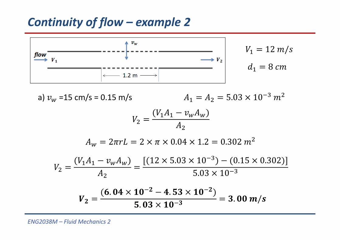
Continuity of flow – example 2Water flowing through an 8 cm diameter pipe enters a porous section which allows a radial velocity through the wall surfaces for a distance of 1.2 metres. If the entrance average velocity is 12 m/s, find the exit average velocity if:

a) is 15 cm/s out of the pipe walls and

b) is 10 cm/s into the pipe.

flow

1.2 m



12 / 80.084 5.03 10

• By continuity,

so

• Rearranging:



a) =15 cm/s = 0.15 m/s 5.03 10

2 2 0.04 1.2 0.302

12 5.03 10 0.15 0.3025.03 10

12 /

8

. .. . /



b) = ‐10 cm/s = ‐0.10 m/s 5.03 10

2 2 0.04 1.2 0.302

12 5.03 10 0.10 0.3025.03 10

12 /

8

. /


Continuity of flow – example 3Surge tank



Surge tank

• A surge tank may be attached to a pressurised pipe flow in order to accommodate sudden changes in pressure.

• It can either absorb sudden rises in pressure or quickly provide extra fluid in case of a drop in pressure.

• Used in all branches of engineering.

• Often found on racing cars undergoing high levels of lateral acceleration to ensure that the inlet to the fuel pump is never starved of fuel.



The pipe flow fills a cylindrical surge tank as shown here. At time t = 0, the water depth in the tank is 30 cm. Estimate the time required to fill the remainder of the tank.

flow . /. /

1 m

d = 12 cm

d = 75 cm

• Firstly calculate pipe areas,

0.124 1.13 10

0.754 4.42 10



1.13 10

4.42 10

2.5 / 1.9 /

• By continuity,

• So,

• Rearrange to find ,



1.13 10

4.42 10

2.5 / 1.9 /

2.5 1.13 10 1.9 1.13 104.42 10

0.02825 0.021470.442 0.01534 /

• So,0.01534 0.442 6.78 10 /



• To fill remainder of tank the water has to rise from 30 cm to 1 metre.

0.754 1 0.3 0.3093

6.78 10 /

• So time to fill remainder of tank,

∆.

. .


Continuity of flow – example 4Jet engine


Pratt and Whitney J52 turbojet engine




At cruise conditions, air flows into a jet engine at a steady rate of 30 kg/s. Fuel enters the engine at a steady rate of 0.3 kg/s. The average velocity of the exhaust gases is 500 m/s relative to the engine. If the engine exhaust effective cross‐sectional area is 0.3 m2 estimate the density of the exhaust gases in kg/m3.

Inlet Exit

Combustion

Thrust

AeAirflow

30 / 0.3 / 500 / 0.3



30 /

0.3 /

500 /

0.3

• By continuity,

30 0.3 30.3 /• And,

• Rearrange, .. . /


The End

fluids 2 lecture 2 - wordpress.com · • no tutorial week 3 ‐3rd october 2013 –this thursday....

Documents