Global urban signatures of phenotypic change inanimal and plant populationsMarina Albertia,1, Cristian Correab, John M. Marzluffc, Andrew P. Hendryd,e, Eric P. Palkovacsf, Kiyoko M. Gotandag,Victoria M. Hunta, Travis M. Apgarf, and Yuyu Zhouh

aDepartment of Urban Design and Planning, University of Washington, Seattle, WA 98195; bInstituto de Conservación, Biodiversidad y Territorio,Universidad Austral de Chile, Casilla 567, Valdivia, Chile; cSchool of Environmental and Forest Sciences, University of Washington, Seattle, WA 98195;dRedpath Museum, McGill University, Montreal, QC, Canada H3A0C4; eDepartment of Biology, McGill University, Montreal, QC, Canada H3A0C4;fDepartment of Ecology and Evolutionary Biology, University of California, Santa Cruz, CA 95060; gDepartment of Zoology, University of Cambridge,Cambridge CB2 3EJ, United Kingdom; and hDepartment of Geological and Atmospheric Sciences, Iowa State University, Ames, IA 50011

Edited by Jay S. Golden, Duke University, Durham, NC, and accepted by Editorial Board Member B. L. Turner October 31, 2016 (received for review August2, 2016)

Humans challenge the phenotypic, genetic, and cultural makeup ofspecies by affecting the fitness landscapes on which they evolve.Recent studies show that cities might play a major role in contem-porary evolution by accelerating phenotypic changes in wildlife,including animals, plants, fungi, and other organisms. Many studiesof ecoevolutionary change have focused on anthropogenic drivers,but none of these studies has specifically examined the role thaturbanization plays in ecoevolution or explicitly examined its mecha-nisms. This paper presents evidence on the mechanisms linking urbandevelopment patterns to rapid evolutionary changes for species thatplay important functional roles in communities and ecosystems.Through a metaanalysis of experimental and observational studiesreporting more than 1,600 phenotypic changes in species across mul-tiple regions, we ask whether we can discriminate an urban signatureof phenotypic change beyond the established natural baselines andother anthropogenic signals. We then assess the relative impact offive types of urban disturbances including habitat modifications,biotic interactions, habitat heterogeneity, novel disturbances, and so-cial interactions. Our study shows a clear urban signal; rates of phe-notypic change are greater in urbanizing systems compared withnatural and nonurban anthropogenic systems. By explicitly linkingurban development to traits that affect ecosystem function, we canmap potential ecoevolutionary implications of emerging patterns ofurban agglomerations and uncover insights for maintaining key eco-system functions upon which the sustainability of human well-being depends.

ecoevolution | urbanization | ecosystem function | sustainability |anthropocene

Emerging evidence of phenotypic change on contemporarytimescales challenges the assumption that evolution only oc-

curs over hundreds or thousands of years. Anthropogenic changesin ecological conditions can drive evolutionary change in speciestraits that can alter ecosystem function (1–3). However, the reciprocaland simultaneous outcomes of such interactions have only begun toemerge (4). Despite increasing evidence that humans are majordrivers of microevolution, the role of human activities in suchdynamics is still unclear. Might human-driven evolution lead toecosystem change with consequences for human well-being withincontemporary timescales (5, 6)?To address this question, human-driven phenotypic change

must be considered in the context of global rapid urbanization.In 1950, 30% of the world’s population lived in urban settle-ments (7). By 2014, that figure had risen to 54%, and by 2050 it isexpected to reach 66% (7). By 2030, urban land cover is forecastto increase by 1.2 million km2, almost tripling the global urbanland area of 2000 (8). Urbanization drives systemic changes tosocioecological systems by accelerating rates of interactionsamong people, multiplying connections among distant places, andexpanding the spatial scales and ecological consequences of hu-man activities to global levels (9).

A critical question for sustainability is whether, on an in-creasingly urbanized planet, the expansion and patterns of urbanenvironments accelerate the evolution of ecologically relevanttraits with potential impacts on urban populations via basic eco-system services such as food production, carbon sequestration, andhuman health. In cities, ecoevolutionary changes are occurring atan unprecedented pace. Humans challenge the phenotypic, ge-netic, and cultural makeup of species on the planet by changingthe fitness landscapes on which they evolve. Examples of con-temporary evolution associated with urbanization have beendocumented for many species (1, 5, 6, 10).This paper examines the mechanisms linking urban development

patterns to contemporary evolutionary changes. Through a meta-analysis of experimental and observational studies that report>1,600 phenotypic changes in many species across multiple regions,we investigated the emergence of distinct signatures of urban-drivenphenotypic change. We hypothesize that shifts in the physical andsocioeconomic structure and function of large urban complexes candrive rapid evolution of many species that play important roles incommunities and ecosystems. Thus, urbanization-driven phenotypicchange may, in turn, impact critical aspects of ecosystem function.We ask the following two questions: (i) Is there evidence of an

urban signature of phenotypic change beyond the establishednatural and anthropogenic signals, accelerating rates of pheno-typic change in species across multiple regions? (ii) What are therelative impacts of five types of urban disturbance: habitat modi-fication, biotic interaction, heterogeneity, novel disturbance, andsocial interaction?

Significance

Ecoevolutionary feedbacks on contemporary timescales werehypothesized over half a century ago, but only recently hasevidence begun to emerge. The role that human activity playsin such dynamics is still unclear. Through a metaanalysis of>1,600 phenotypic changes in species across regions and eco-system types, we examine the evidence that the rate of phe-notypic change has an urban signature. Our findings indicategreater phenotypic change in urbanizing systems comparedwith natural and nonurban anthropogenic systems. By explic-itly linking urban development to trait changes that might af-fect ecosystem function, we provide insights into the potentialecoevolutionary implications for maintaining ecosystem func-tion and the sustainability of human well-being.

Author contributions: M.A., C.C., J.M.M., A.P.H., E.P.P., K.M.G., and V.M.H. designed re-search; M.A., A.P.H., E.P.P., K.M.G., V.M.H., T.M.A., and Y.Z. performed research; C.C.analyzed data; and M.A., C.C., J.M.M., A.P.H., E.P.P., K.M.G., and V.M.H. wrote the paper.

The authors declare no conflict of interest.

This article is a PNAS Direct Submission. J.S.G. is a Guest Editor invited by the EditorialBoard.1To whom correspondence should be addressed. Email: malberti@uw.edu.

This article contains supporting information online at www.pnas.org/lookup/suppl/doi:10.1073/pnas.1606034114/-/DCSupplemental.

www.pnas.org/cgi/doi/10.1073/pnas.1606034114 PNAS Early Edition | 1 of 6

SUST

AINABILITY

SCIENCE

EVOLU

TION

SPEC

IALFEATU

RE

Our hypothesis is grounded in the growing evidence that ur-banization is a major driver of contemporary evolution. Urbandevelopment changes habitat structure (i.e., loss of forest coverand connectivity), processes (i.e., biogeochemical and nutrientcycling), and biotic interactions (i.e., predation) (6). Humans incities mediate ecoevolutionary interactions by introducing noveldisturbances and altering habitat heterogeneity. Urban environ-ments can facilitate hybridization by reducing reproductive iso-lation (11). They can also isolate populations through habitatfragmentation (12). In addition to changes in the physical tem-plate, humans in cities modify the availability of resources andtheir variability over time, buffering their effects on communitystructure (12). Complex interactions resulting from changes inhabitat and biotic interactions coupled with emerging spatial andtemporal patterns of resource availability might produce newevolutionary dynamics and feedbacks. Furthermore, in cities, therapid pace of change associated with increasing social interac-tions amplifies the impacts of human agency, both locally and ata distance (telecoupling). Understanding how urban-driven con-temporary evolution affects ecosystem functions will provide in-sights for maintaining biodiversity and achieving global urbansustainability.

ResultsWe discriminated the emergence of distinct signatures of ur-banization by statistically modeling phenotypic change as afunction of urban disturbances, urban proximity, and other po-tentially relevant previously identified variables. Using generalizedlinear mixed-effect models (GLMMs), in an information-theoreticframework to enforce parsimony and acknowledge model un-certainty, we analyzed a modified and georeferenced version ofa database of rates of phenotypic change that has been developedover two decades (5, 13–17). After a series of quality filters, weretained for analyses 89 studies targeting 155 species, 175 studysystems, and >1,600 rates of phenotypic change (Fig. 1) (SI Appendix,Database Filtering).Statistical models including urban variables outperformed

models lacking urban variables, while accounting for anthropo-genic context and other putatively important variables describedbelow. Hendry et al. (15) showed that organisms in an anthro-pogenic context (e.g., pollution, overharvest) had higher rates ofphenotypic change compared with those in a natural context. Itwas unclear whether urban variables would add explanatory powerafter statistically controlling for the anthropogenic context. Ourresults showed that urban variables provide substantial additionalinformation explaining phenotypic change, thus warranting further

consideration (SI Appendix, Gauging the Urban Signature Beyondthe Anthropogenic Context).The multifarious effects of urban agglomerations occur across

multiple spatial scales (9). Hence, we considered both variablesdetermined by location relative to urban agglomerations andurban-driven processes regardless of location. Urban predictorvariables included Urban Disturbance (categorical, seven classesof urban-related mechanisms plus one reference natural state),City Lights (ordinal, ranging from 0 to 1—wildland to city),Anthropogenic Biome (ordinal, ranging from 1 to 6—dense set-tlements to wildlands), and Urbanization (difference in Anthro-pogenic Biome between years 1900 and 2000) (SI Appendix, UrbanDisturbance Classification). Because some phenotypic changes weremeasured from populations at two locations (see Design), contin-uous and ordinal predictor variables were calculated both as meanand Δ (difference) between the two samples underlying a pheno-typic change. This analysis included six urban variables represent-ing a range of possible mechanisms, scales, and proxies of urbandrivers of phenotypic change (Materials and Methods). We alsoincluded three unrelated background variables that may affectphenotypic change (13–15): (i) number of Generations (continuous,log-transformed); (ii) whether the phenotypic change was estimatedfrom a longitudinal or cross-sectional study Design (categori-cal, two classes—allochronic and synchronic); and (iii) whetherthe phenotypic change had a demonstrated genetic basis ornot (labeled GenPhen, categorical, two classes—genotypic andphenotypic).We conducted exploratory multimodel ranking and inference

based on second-order Akaike information criteria (AICc) toevaluate the relative ability of urban and background variablesto statistically explain the absolute magnitude of standardizedphenotypic change, and to assess effect sizes averaged over allpossible models (18). A large model set (512 models) was createdby considering all combinations of the nine explanatory variablesin the fixed part of the GLMM (Materials and Methods and SIAppendix, Materials and Methods—Statistical Analysis). The ran-dom part of all models was held constant, and included a randomintercept per Study System to account for nested data structure,and a previously selected variance function that allowed the re-sidual variance to scale with the expected response. Phenotypicchange (square-rooted) was the response variable, measured asthe absolute magnitude of phenotypic change standardized bycharacter variation, a quantity known as Haldane numerator (19).Top-ranked models consistently included urban variables. For

example, the focal variables Urban Disturbance, City Lights, andAnthrobiome are prevalent in top-ranked models and in the 95%confidence set, whereas, among background variables, Generations

Urban Disturbance:Other: Natural

Habitat Modifica�on Heterogeneity Bio�c Interac�on Social Interac�on Novel Disturbance

Fig. 1. Global distribution of study sys-tems of trait changes in wild populations.Symbols represent Urban Disturbances,wherein each study system is categorizedaccording to its primary driver of pheno-typic trait change. White regions representCity Lights. Background of the Earth in 2012from NASA: earthobservatory.nasa.gov/Features/NightLights/page3.php.

2 of 6 | www.pnas.org/cgi/doi/10.1073/pnas.1606034114 Alberti et al.

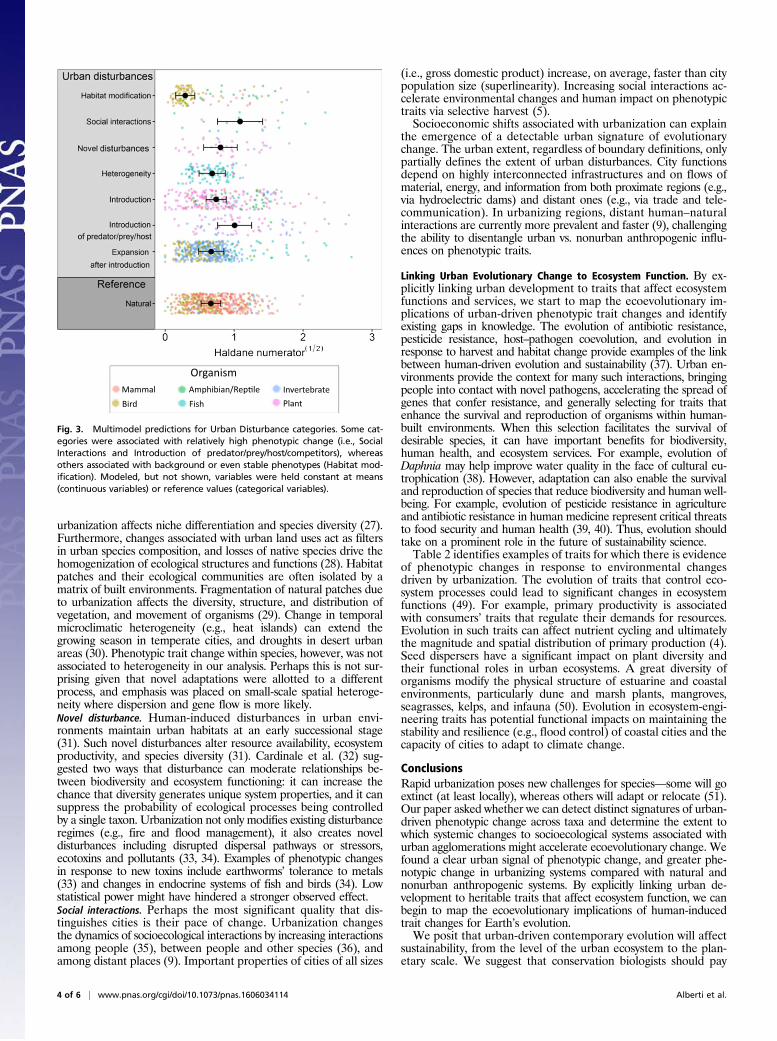
and GenPhen were prevalent (Fig. 2). Model-averaged partial re-gression coefficients (incorporating model uncertainty) revealedseveral strong and many weak effects (Table 1). Among urban-related variables, phenotypic changes estimated from contrasts be-tween urban vs. wild habitats (i.e., Δ City Lights) were higher thancontrasts within either urban or wild habitats. Mean City Lights,however, showed only a marginally significant effect (P < 0.1).Urbanization, inferred from land cover change during the lastcentury (mean Urbanization, with negative scores representing ur-banization) showed a trend with highest rates of phenotypic changein urbanizing locations. This trend was not supported by the effect ofcontemporary land cover (Anthrobiome). Urban Disturbance hadseveral effects. For example, social interactions, and introduction ofpredators, prey, hosts, or competitors, were associated with relativelyhigh phenotypic change. Some effects were counterintuitive, for ex-ample, habitat modification was associated with relatively low phe-notypic change. The effects of Urban Disturbance were furtherillustrated by multimodel predictions made while the effects of othervariables were statistically held constant (Fig. 3). The range of effectsattributed to Urban Disturbance on multimodel predictions weresubstantial compared with those of different combinations of back-ground variables (SI Appendix, Database Filtering).

DiscussionOur results show a clear urban signal of phenotypic change andreveal variable effects of urban disturbance mechanisms. Observedeffects might be due to the multiple challenges that urbanizationposes on adaptation. Multiple influences can increase the totalstrength of selection on a trait, or the number of traits under se-lection (20).

Urban Disturbance Mechanisms. Urban Disturbance representscoupled mechanisms through which urban development affectsnatural processes and evolutionary dynamics. Model predictionshighlight two categories driving the urban signature: social interac-tions and biotic interactions, specifically introduction of predators,prey, hosts, and competitors. Anthropogenic habitat modificationhad a lower than expected impact. The assessment of the effect of

the various urban disturbances should be interpreted cautiouslysince it might reflect the classification of interrelated disturbances,and the nature of species observed in available studies.Habitat modification. Land cover conversion and loss of nativehabitat are major drivers of contemporary evolution. The ob-served counterintuitive lower phenotypic change associated withHabitat Modification relative to the Natural context in our studymay reflect in part the vagility of birds generally, and an over-representation in the database of studies finding stable migrationphenology of European birds in particular. It also might be dueto the fact that habitat modification is captured by other in-terrelated urban disturbance classes and by other variables suchas Δ City Lights that show the expected trend of greater phe-notypic change. Urban-driven habitat modification can affectspecies traits and composition. For example, changes in climate,artificial lighting, and availability of food are all drivers of changein the timing and duration of reproduction in some bird species(21). Changes in productivity—the rate at which energy flowsthrough an ecosystem—might explain species diversity patternsalong the urban–rural gradient (22).Biotic interactions. We determined that introduction of predator,prey, host, or competition contributes to a higher rate of pheno-typic change compared with range expansion after introductionor introduction alone. Urban development creates new oppor-tunities and challenges for species competition and predation,both as exotic species are introduced and as invasive speciesmigrate in, taking advantage of poorly integrated communitiesand patches. This might result in colonization, as more frequentintroductions of exotic species translate into invasions (23). Forexample, McDonnell and Hahs (24) found higher levels of earth-worm biomass and abundance in urban forests compared withrural ones, likely because of introduced species. Urbanizationalso alters the way species distribute and interact (25). Marzluff(25) found that, although diversity still emerges as the balancebetween extinction and colonization, species invasion plays aprominent role.Heterogeneity. At the community level, cities directly and indirectlyaffect phenotypic change by altering spatial and temporal habitatheterogeneity. Increasing evidence supports the hypothesis thaturban regions amplify heterogeneity by the intensity and speed ofhuman-biophysical and social interactions (26). Cities worldwideretain native species, but loss of functional heterogeneity driven by

Importance of predictor

Low

High

Model 1

Model 2Etc.

evitalumuC

ekiak A( thgie

wω

)

0.0

0.2

0.4

0.6

0.8

1.0

Condi�onal probabili�es

Fig. 2. Representation of the AICc model selection table. Rows representmodels sorted by decreasing empirical support (row height represents modelprobability conditional on the full model set). Predictor variables wereshaded if included in a model. Saturation corresponded to estimated vari-able relative importance. Note all high-ranked models contained urban(e.g., Urban Disturbance) and background variables (e.g., Generations).Models with little relative support were omitted for clarity (95% confidenceset displayed).

Table 1. Model-averaged coefficients from the full model setrevealed several strong and many weak effects

Parameter† Estimate SE Z score P value

(Intercept) 0.545 0.097 5.619 0.000***Generations 0.032 0.015 2.22 0.026*Design—Synchronic 0.034 0.065 0.528 0.597GenPhen—Phenotypic 0.104 0.052 2.006 0.045*Mean City Lights 0.056 0.033 1.695 0.090·

Δ City Lights 0.072 0.031 2.344 0.019*Mean Anthrobiome −0.009 0.008 1.141 0.254Δ Anthrobiome −0.002 0.009 0.216 0.829Mean Urbanization −0.014 0.008 1.799 0.072·

U. Dist.—Hetero 0.019 0.097 0.200 0.841U. Dist.—HabMod −0.371 0.046 8.088 0.000***U. Dist.—Novel 0.14 0.136 1.028 0.304U. Dist.—Social 0.425 0.154 2.753 0.006**U. Dist.—Int 0.077 0.073 1.061 0.289U. Dist.—IntEco 0.345 0.126 2.738 0.006**U. Dist.—ExpaInt 0.005 0.09 0.059 0.953

Significance levels: ***P < 0.001, **P < 0.01, *P < 0.05, ·P < 0.1.†Abbreviations: U. Dist., Urban Disturbance; HabMod, habitat modification;Hetero, heterogeneity; and subcategories of biotic interaction: Int, intro-duction; IntEco, introduction of predator/prey/host/competition; Expalnt,range expansion after introduction.

Alberti et al. PNAS Early Edition | 3 of 6

SUST

AINABILITY

SCIENCE

EVOLU

TION

SPEC

IALFEATU

RE

urbanization affects niche differentiation and species diversity (27).Furthermore, changes associated with urban land uses act as filtersin urban species composition, and losses of native species drive thehomogenization of ecological structures and functions (28). Habitatpatches and their ecological communities are often isolated by amatrix of built environments. Fragmentation of natural patches dueto urbanization affects the diversity, structure, and distribution ofvegetation, and movement of organisms (29). Change in temporalmicroclimatic heterogeneity (e.g., heat islands) can extend thegrowing season in temperate cities, and droughts in desert urbanareas (30). Phenotypic trait change within species, however, was notassociated to heterogeneity in our analysis. Perhaps this is not sur-prising given that novel adaptations were allotted to a differentprocess, and emphasis was placed on small-scale spatial heteroge-neity where dispersion and gene flow is more likely.Novel disturbance. Human-induced disturbances in urban envi-ronments maintain urban habitats at an early successional stage(31). Such novel disturbances alter resource availability, ecosystemproductivity, and species diversity (31). Cardinale et al. (32) sug-gested two ways that disturbance can moderate relationships be-tween biodiversity and ecosystem functioning: it can increase thechance that diversity generates unique system properties, and it cansuppress the probability of ecological processes being controlledby a single taxon. Urbanization not only modifies existing disturbanceregimes (e.g., fire and flood management), it also creates noveldisturbances including disrupted dispersal pathways or stressors,ecotoxins and pollutants (33, 34). Examples of phenotypic changesin response to new toxins include earthworms’ tolerance to metals(33) and changes in endocrine systems of fish and birds (34). Lowstatistical power might have hindered a stronger observed effect.Social interactions. Perhaps the most significant quality that dis-tinguishes cities is their pace of change. Urbanization changesthe dynamics of socioecological interactions by increasing interactionsamong people (35), between people and other species (36), andamong distant places (9). Important properties of cities of all sizes

(i.e., gross domestic product) increase, on average, faster than citypopulation size (superlinearity). Increasing social interactions ac-celerate environmental changes and human impact on phenotypictraits via selective harvest (5).Socioeconomic shifts associated with urbanization can explain

the emergence of a detectable urban signature of evolutionarychange. The urban extent, regardless of boundary definitions, onlypartially defines the extent of urban disturbances. City functionsdepend on highly interconnected infrastructures and on flows ofmaterial, energy, and information from both proximate regions (e.g.,via hydroelectric dams) and distant ones (e.g., via trade and tele-communication). In urbanizing regions, distant human–naturalinteractions are currently more prevalent and faster (9), challengingthe ability to disentangle urban vs. nonurban anthropogenic influ-ences on phenotypic traits.

Linking Urban Evolutionary Change to Ecosystem Function. By ex-plicitly linking urban development to traits that affect ecosystemfunctions and services, we start to map the ecoevolutionary im-plications of urban-driven phenotypic trait changes and identifyexisting gaps in knowledge. The evolution of antibiotic resistance,pesticide resistance, host–pathogen coevolution, and evolution inresponse to harvest and habitat change provide examples of the linkbetween human-driven evolution and sustainability (37). Urban en-vironments provide the context for many such interactions, bringingpeople into contact with novel pathogens, accelerating the spread ofgenes that confer resistance, and generally selecting for traits thatenhance the survival and reproduction of organisms within human-built environments. When this selection facilitates the survival ofdesirable species, it can have important benefits for biodiversity,human health, and ecosystem services. For example, evolution ofDaphnia may help improve water quality in the face of cultural eu-trophication (38). However, adaptation can also enable the survivaland reproduction of species that reduce biodiversity and human well-being. For example, evolution of pesticide resistance in agricultureand antibiotic resistance in human medicine represent critical threatsto food security and human health (39, 40). Thus, evolution shouldtake on a prominent role in the future of sustainability science.Table 2 identifies examples of traits for which there is evidence

of phenotypic changes in response to environmental changesdriven by urbanization. The evolution of traits that control eco-system processes could lead to significant changes in ecosystemfunctions (49). For example, primary productivity is associatedwith consumers’ traits that regulate their demands for resources.Evolution in such traits can affect nutrient cycling and ultimatelythe magnitude and spatial distribution of primary production (4).Seed dispersers have a significant impact on plant diversity andtheir functional roles in urban ecosystems. A great diversity oforganisms modify the physical structure of estuarine and coastalenvironments, particularly dune and marsh plants, mangroves,seagrasses, kelps, and infauna (50). Evolution in ecosystem-engi-neering traits has potential functional impacts on maintaining thestability and resilience (e.g., flood control) of coastal cities and thecapacity of cities to adapt to climate change.

ConclusionsRapid urbanization poses new challenges for species—some will goextinct (at least locally), whereas others will adapt or relocate (51).Our paper asked whether we can detect distinct signatures of urban-driven phenotypic change across taxa and determine the extent towhich systemic changes to socioecological systems associated withurban agglomerations might accelerate ecoevolutionary change. Wefound a clear urban signal of phenotypic change, and greater phe-notypic change in urbanizing systems compared with natural andnonurban anthropogenic systems. By explicitly linking urban de-velopment to heritable traits that affect ecosystem function, we canbegin to map the ecoevolutionary implications of human-inducedtrait changes for Earth’s evolution.We posit that urban-driven contemporary evolution will affect

sustainability, from the level of the urban ecosystem to the plan-etary scale. We suggest that conservation biologists should pay

OrganismMammalBird

Amphibian/Rep�leFish

InvertebratePlant

Fig. 3. Multimodel predictions for Urban Disturbance categories. Some cat-egories were associated with relatively high phenotypic change (i.e., SocialInteractions and Introduction of predator/prey/host/competitors), whereasothers associated with background or even stable phenotypes (Habitat mod-ification). Modeled, but not shown, variables were held constant at means(continuous variables) or reference values (categorical variables).

4 of 6 | www.pnas.org/cgi/doi/10.1073/pnas.1606034114 Alberti et al.

increased attention to mechanisms by which the emergent humanhabitat influences population persistence (4). Such understandingwill provide insights for maintaining ecosystem function in thelong term and can direct policy makers toward sustainability so-lutions (37).

Materials and MethodsDatabase on Rates of Phenotypic Change. We improved an existing databaseon rates of phenotypic change (5, 13–17). We added new data published upto August of 2015. Studies were surveyed by searching ISI Web of Science,Google Scholar, and cross-references, using ad hoc keywords (e.g., quanti-tative trait, evolutionary change, rapid evolution, ecoevolutionary, anthro-pogenic change, urban disturbances, and system stability). Studies werescreened (SI Appendix, Database Filtering), and, if selected, phenotypic rateswere extracted (Statistical Analyses) and classified according to qualities ofthe study system including ecological and anthropogenic contexts (5). Eachrow corresponded to one phenotypic change rate estimate and associatedcontextual attributes including type of study: allochronic for longitudinalstudies, or synchronic for cross-sectional studies comparing samples obtainedsynchronously from populations derived from a common ancestral pop-ulation. Rates were classified according to whether phenotypic change couldbe attributed to quantitative genetic effects (Genetic), or could not be dis-tinguished from phenotypic plasticity (Phenotypic). Generations was calcu-lated as the number of years between population samples (or since populationdivergence, if synchronic) divided by expected generation time.

The dataset had a hierarchical structure, with variable numbers ofphenotypic change estimates (from different morphological characters andor populations) within study systems, species, and taxa. Study system wasdefined as population(s) of a species within a geographical region puta-tively exposed to similar environmental effects and high gene flow potential.We evaluated whether study systems were evolving in an anthropo-genic vs. natural context (15), and the effect of Urban Disturbance (seenext section).

Urban Disturbance Classification and Georeferencing.We use the global urbanarea map at 1-km spatial resolution developed by Zhou et al. (52). The mapis based on a cluster-based method to estimate optimal thresholds formapping urban extent using DMSP/OLS NTL to account for regional vari-ations in urban clusters (53). The anthropogenic biome of all samples wasbased on the Anthropogenic Biomes geodataset for the year 2000 (54).

For samples in study systems in which the driver of evolutionary change isanthropogenic, we classify the Urban Disturbance as social interaction, biotic

interaction, habitat modification, heterogeneity, or novel disturbance (6) (SIAppendix, Urban Disturbance Classification). Habitat modification repre-sents changes in climate, modification of the landscape, or pollution. Bioticinteractions stem from introductions, and are subcategorized depending onthe study organism’s ecological role: introduced species vs. species in itsnative range responding to an introduction. Introduced species are furtherdivided into species in a new range following introduction vs. introducedspecies after range expansion. Heterogeneity can refer to heterogeneity inspace or time. Novel disturbances require novel adaptations, for example,rapid evolution of zinc tolerance (42). Social interactions refer to direct orintentional results of human agency. Examples are listed in Table 2.

Statistical Analyses. We used an information-theoretic approach to rankstatistical models and conduct multimodel inference, based on AICc(23, 55). AICc favors model fit (minimizing deviance) while avoidingmodel overfitting (penalizing for the number of estimated parameters,K ), and was the basis for enforcing the parsimony principle given oursample sizes (1,663 rates nested in 175 study systems). The statisticalmodels were GLMMs. The response variable, phenotypic change (square-root transformed), was measured as the absolute magnitude of pheno-typic change standardized by character variation (Haldane numerator;ref. 19, as formulated in ref. 13). The square-root transformation mini-mized patterns in adjusted residuals plots in preliminary analyses. Be-cause the data had a hierarchical structure, study system was alwaysmodeled as a random effect, with combinations of background and urbanvariables (fixed effects):

Hð1=2ÞðiÞ = αjðiÞ + βχ i + «i ,

αj ∼Ν�μ, σ2α

�,

«∼Nð0,fðγÞÞ,

where the indexes i run from 1 to number of observations, and j run from 1 tonumber of study systems, H(1/2) is the response variable (square-root ofHaldane numerator), α is normally distributed with mean μ (overall in-tercept) and variance σ2α, allowing for varying intercepts per study system, βis a vector of partial regression coefficients related to a matrix of explana-tory variables X, and « is the residual error with variance γ, which wasmodeled as follows:

γ= 0.1494*�C + jfittedjP

�2,

where C is a constant by stratum (0.3233 for genetic; 0.1249 for phenotypic),and P is an exponent of absolute fitted values by stratum (2.0754 for genetic;

Table 2. Mapping urban-driven phenotypic trait change to ecosystem function

Urban signatures Ecoevolutionary feedback

Urban Disturbance Mechanism Phenotypic trait Ecosystem function Feedback mechanism Ref.

PhysiologicalNovel Exposure to effluent/heat

from power plantHeat coma temp.

(thermal tolerance) insnails (Physa virgata)

Biodiversity New “physiological races”;colonization

41

Novel Electricity pylons, novelhigh-zinc habitats

Zinc tolerance in plants: Agrostiscapillaris, Agrostis stolonifera, etc.

Primary productivity;biodiversity

Consumer–resourcedynamics

42

MorphologicalHeterogeneity Hydrological connectivity

altered via a fish ladderBody size in brown trout

(Salmo trutta)Nutrient cycling Life history changes 43

Biotic interaction Invasion of a molluskivorouscrab (Carcinus maenas)

Shell thickness (in millimeters) inperiwinkle snail (Littorina obtusta)

Biotic control Trophic interactions 44

Social interaction Long-term selective harvestingof a medicinal plant

Size of American ginseng plants(Panax quinquefolius)

Primary productivity;biodiversity

Consumer–resourcedynamics

45

BehavioralBiotic interaction Introduction to

predator-free islandAntipredator behavior in multiple

species of marsupialsNutrient cycling Allocation of time to

foraging vs. vigilance46

Phenological/life historyHeterogeneity Temporal heterogeneity

in water availabilityFlowering time in field mustard

(Brassica rapa)Primary production Consumer–resource

dynamics47

Habitatmodification

Global climate change Seasonal onset of reproductionin 65 species of migratory birds

Biodiversity;biotic control

Colonization; novelcompetition

48

Documented phenotypic trait changes (see ref.), urban drivers, and hypothesized ecoevolutionary feedback mechanisms.

Alberti et al. PNAS Early Edition | 5 of 6

SUST

AINABILITY

SCIENCE

EVOLU

TION

SPEC

IALFEATU

RE

1.2376 for phenotypic). Hence, the chosen residual variance increased expo-nentially with fitted values, and slightly more so in genetic than phenotypicrates (SI Appendix, Materials and Methods—Statistical Analysis).

We used exploratory multimodel inference to assess the relative impor-tance of predictor variables for phenotypic change, and to make predictionsabout contrasting urban-related scenarios that considered informationcontained in all models. From three background plus six urban variables, wecombined nine predictor variables to form 29 = 512 models, including a nullmodel (intercept only), and excluding interactions. All models were fittedthrough maximum likelihood in the R package nlme (56). Models wereranked according to decreasing values of AICc (57), and further evaluatedusing standard methods after refitting through restricted maximum-likeli-hood estimation (58). Predictor variable relative importance was calculated

by the sum of the Akaike weights of all models containing a particularpredictor variable. Similarly, model-averaged partial regression coefficientswere Akaike-weighted averages of coefficients from all models containing aparticular term (18). Model ranking and inference was conducted in the Rpackage MuMin, version 1.15.6 (55) (SI Appendix, Materials and Methods—Statistical Analysis).

ACKNOWLEDGMENTS. We thank the John D. and Catherine T. MacArthurFoundation for partially supporting the study (Grant 14-106477-000-USP). C.C.was funded by Comisión Nacional de Investigación Científica y Tecnológica-Programa de Atracción e Inserción de Capital Humano Avanzado (CONICYT-PAI) Grant 82130009 and Fondo Nacional de Desarrollo Científico y Tecnológico(FONDECYT) Grant 11150990.

1. Post DM, Palkovacs EP (2009) Eco-evolutionary feedbacks in community and ecosys-tem ecology: Interactions between the ecological theatre and the evolutionary play.Philos Trans R Soc Lond B Biol Sci 364(1523):1629–1640.

2. Pimentel D (1961) Animal population regulation by the genetic feed-back mecha-nism. Am Nat 95(881):65–79.

3. Schoener TW (2011) The newest synthesis: Understanding the interplay of evolu-tionary and ecological dynamics. Science 331(6016):426–429.

4. Matthews B, et al. (2011) Toward an integration of evolutionary biology and eco-system science. Ecol Lett 14(7):690–701.

5. Palkovacs EP, Kinnison MT, Correa C, Dalton CM, Hendry AP (2012) Fates beyondtraits: Ecological consequences of human-induced trait change. Evol Appl 5(2):183–191.

6. Alberti M (2015) Eco-evolutionary dynamics in an urbanizing planet. Trends Ecol Evol30(2):114–126.

7. United Nations, Department of Economic and Social Affairs, Population Division(2014) World Urbanization Prospects: The 2014 Revision: Highlights (ST/ESA/SER.A/352) (Department of Economic and Social Affairs, Population Division, United Na-tions, New York).

8. Seto KC, Güneralp B, Hutyra LR (2012) Global forecasts of urban expansion to 2030and direct impacts on biodiversity and carbon pools. Proc Natl Acad Sci USA 109(40):16083–16088.

9. Liu J, et al. (2013) Framing sustainability in a telecoupled world. Ecol Soc 18(2):26.10. Marzluff JM, Angell T (2005) Cultural coevolution: How the human bond with crows

and ravens extends theory and raises new questions. J Ecol Anthropol 9(1):69–75.11. Hasselman DJ, et al. (2014) Human disturbance causes the formation of a hybrid

swarm between two naturally sympatric fish species. Mol Ecol 23(5):1137–1152.12. Partecke J (2013) Mechanisms of phenotypic responses following colonization of ur-

ban areas: From plastic to genetic adaptation. Avian Urban Ecology: Behavioural andPhysiological Adaptations, eds Gil D, Brumm H (Oxford Univ Press, Oxford, UK), p 131.

13. Hendry AP, Kinnison MT (1999) Perspective: The pace of modern life: Measuring ratesof contemporary microevolution. Evolution 53(6):1637–1653.

14. Kinnison MT, Hendry AP (2001) The pace of modern life II: From rates of contem-porary microevolution to pattern and process. Genetica 112-113:145–164.

15. Hendry AP, Farrugia TJ, Kinnison MT (2008) Human influences on rates of phenotypicchange in wild animal populations. Mol Ecol 17(1):20–29.

16. Crispo E, et al. (2010) The evolution of phenotypic plasticity in response to anthro-pogenic disturbance. Evol Ecol Res 12(1):47–66.

17. Gotanda KM, Correa C, Turcotte MM, Rolshausen G, Hendry AP (2015) Linking mac-rotrends and microrates: Re-evaluating microevolutionary support for Cope’s rule.Evolution 69(5):1345–1354.

18. Anderson DR (2008) Model Based Inference in the Life Sciences: A Primer on Evidence(Springer, New York), 1st Ed.

19. Haldane JB (1949) Suggestions as to quantitative measurement of rates of evolution.Evolution 3(1):51–56.

20. Nosil P, Harmon LJ, Seehausen O (2009) Ecological explanations for (incomplete)speciation. Trends Ecol Evol 24(3):145–156.

21. Winkel W, Hudde H (1997) Long-term trends in reproductive traits of tits (Parusmajor, P. caeruleus) and pied flycatchers Ficedula hypoleuca. J Avian Biol 28(2):187–190.

22. Mittelbach GG, et al. (2001) What is the observed relationship between speciesrichness and productivity? Ecology 82(9):2381–2396.

23. Faeth SH, Warren PS, Shochat E, Marussich WA (2005) Trophic dynamics in urbancommunities. Bioscience 55(5):399–407.

24. McDonnell M, Hahs A (2008) The use of gradient analysis studies in advancing ourunderstanding of the ecology of urbanizing landscapes: Current status and futuredirections. Landsc Ecol 23(10):1143–1155.

25. Marzluff JM (2005) Island biogeography for an urbanizing world: How extinction andcolonization may determine biological diversity in human-dominated landscapes.Urban Ecosyst 8(2):157–177.

26. Pickett STA, et al. (2016) Dynamic heterogeneity: A framework to promote ecologicalintegration and hypothesis generation in urban systems. Urban Ecosyst, in press.

27. Aronson MFJ, et al. (2014) A global analysis of the impacts of urbanization on birdand plant diversity reveals key anthropogenic drivers. Proc R Soc B 281(1780):20133330.

28. Groffman PM, et al. (2014) Ecological homogenization of urban USA. Front EcolEnviron 12(1):74–81.

29. Rebele F (1994) Urban ecology and special features of urban ecosystems. Glob EcolBiogeogr 4(6):173–187.

30. Shochat E, Warren PS, Faeth SH, McIntyre NE, Hope D (2006) From patterns toemerging processes in mechanistic urban ecology. Trends Ecol Evol 21(4):186–191.

31. Pickett STA, Wu J, Cadenasso ML (1999) Patch dynamics and the ecology of disturbedground: A framework for synthesis. Ecosystems of Disturbed Ground, ed Walker LR(Elsevier Science, Amsterdam).

32. Cardinale BJ, Hillebrand H, Charles DF (2006) Geographic patterns of diversity instreams are predicted by a multivariate model of disturbance and productivity. J Ecol94(3):609–618.

33. Kille P, et al. (2013) DNA sequence variation and methylation in an arsenic tolerantearthworm population. Soil Biol Biochem 57:524–532.

34. Shenoy K, Crowley PH (2011) Endocrine disruption of male mating signals: Ecologicaland evolutionary implications. Funct Ecol 25(3):433–448.

35. Bettencourt LMA (2013) The origins of scaling in cities. Science 340(6139):1438–1441.36. Clucas B, Marzluff JM (2012) Attitudes and actions toward birds in urban areas: Hu-

man cultural differences influence bird behavior. Auk 129(1):8–16.37. Carroll SP, et al. (2014) Applying evolutionary biology to address global challenges.

Science 346(6207):1245993.38. Chislock MF, Sarnelle O, Jernigan LM, Wilson AE (2013) Do high concentrations of

microcystin prevent Daphnia control of phytoplankton? Water Res 47(6):1961–1970.39. Gluckman PD, Low FM, Buklijas T, Hanson MA, Beedle AS (2011) How evolutionary

principles improve the understanding of human health and disease. Evol Appl 4(2):249–263.

40. Thrall PH, et al. (2011) Evolution in agriculture: The application of evolutionary ap-proaches to the management of biotic interactions in agro-ecosystems. Evol Appl4(2):200–215.

41. McMahon RF (1976) Effluent-induced interpopulation variation in the thermal tol-erance of Physa virgata Gould. Comp Biochem Physiol A 55(1):23–28.

42. Al-Hiyaly SAK, McNeilly T, Bradshaw AD (1990) The effect of zinc contamination fromelectricity pylons. Contrasting patterns of evolution in five grass species. New Phytol114(2):183–190.

43. Haugen TO, Aass P, Stenseth NC, Vøllestad LA (2008) Changes in selection and evo-lutionary responses in migratory brown trout following the construction of a fishladder. Evol Appl 1(2):319–335.

44. Trussell GC, Smith LD (2000) Induced defenses in response to an invading crabpredator: An explanation of historical and geographic phenotypic change. Proc NatlAcad Sci USA 97(5):2123–2127.

45. McGraw JB (2001) Evidence for decline in stature of American ginseng plants fromherbarium specimens. Biol Conserv 98(1):25–32.

46. Blumstein DT, Daniel JC (2003) Foraging behavior of three Tasmanian macropodidmarsupials in response to present and historical predation threat. Ecography 26(5):585–594.

47. Franks SJ, Sim S, Weis AE (2007) Rapid evolution of flowering time by an annual plantin response to a climate fluctuation. Proc Natl Acad Sci USA 104(4):1278–1282.

48. Jenni L, Kéry M (2003) Timing of autumn bird migration under climate change: Ad-vances in long-distance migrants, delays in short-distance migrants. Proc Biol Sci270(1523):1467–1471.

49. Odling-Smee FJ, Laland KN, Feldman MW (2003) Niche Construction: The NeglectedProcess in Evolution (Princeton Univ Press, Princeton).

50. Bouma TJ, De Vries MB, Herman PMJ (2010) Comparing ecosystem engineering effi-ciency of two plant species with contrasting growth strategies. Ecology 91(9):2696–2704.

51. Marzluff JM (2012) Urban evolutionary ecology. Stud Avian Biol 45:287–308.52. Zhou Y, et al. (2015) A global map of urban extent from nightlights. Environ Res Lett

10(5):54011.53. Zhou Y, et al. (2014) A cluster-based method to map urban area from DMSP/OLS

nightlights. Remote Sens Environ 147:173–185.54. Ellis EC, Ramankutty N (2008) Putting people in the map: Anthropogenic biomes of

the world. Front Ecol Environ 6(8):439–447.55. Barton K (2016) Package “MuMIn”: Multi-Model Inference. R package, Version 1.15.6.

Available at https://cran.r-project.org/web/packages/MuMIn/MuMIn.pdf. AccessedAugust 9, 2016.

56. Pinheiro J, Bates D, DebRoy S, Heisterkamp S, Van Willigen B (2016) Package “nlme.”Available at https://cran.r-project.org/web/packages/nlme/nlme.pdf. Accessed August5, 2016.

57. Burnham KP, Anderson DR (2003) Model Selection and Multimodel Inference: APractical Information-Theoretic Approach (Springer, New York), 2nd Ed.

58. Zuur AF, ed (2009) Mixed Effects Models and Extensions in Ecology with R (Springer,New York).

6 of 6 | www.pnas.org/cgi/doi/10.1073/pnas.1606034114 Alberti et al.

1    

Supporting Information

Global urban signatures of phenotypic change in animal and plant populations

Marina Alberti et al.. (1)  (2)  (3)  (4)  (5)  (6)  (7)  (8)  (9)  (10)  (11)  (12)  (13)  (14)  (15)(16)  (17)  (18)  (19)  (20)  (21)  (22)  (23)  (24)  (25)  (26)  (27)  (28)  (29)  (30)(31)  (32)  (33)  (34)  (35)  (36)  (37)  (38)    (39)    (40)  (41)  (42)  (43)  (44)  (45)  (46)    (47)  (48)  (49)  (50)  (51)  (52)  (53)  (54)  (55)  (56)  (57)  (58)    

Contents 1. Database filtering ........................................................................................................................................................... 1

2. Urban Disturbance Classification .............................................................................................................................. 4

3. Gauging the urban signature beyond the anthropogenic context .............................................................. 5

4. Materials and Methods – Statistical analysis .................................................................................................... 10

1. Database filtering We analyzed a modified and geo-referenced version of a database of rates of phenotypic change (5, 13–17). After a series of quality filters, we retained for analyses 89 suitable studies targeting 155 species, 175 study systems, and >1600 rates of phenotypic change (Figure S1). Since the objective of this study was to conduct exploratory statistical analyses to gauge the potential effects of urbanization on an organism's phenotypic change, we focused on a small subset of the original database for which minimum necessary information was available. We further reduced the data set in an attempt to achieve fair comparisons (i.e., unbiased model coefficient estimates). Thus, the database was subjected to a series of filters before conducting the statistical analyses (Table S1).

We began with version V4.04 of the database, which included >11 thousand rates nested in 379 study systems, and 309 species reported in 146 studies. First, the number of rates was reduced by about half by excluding pairwise allochronic contrasts while retaining the first and last samples of each time series. We did not want the analyses to be dominated by a few, long time series. Then we retained rates measured in the range of [1, 300] generations, which allowed the retention of most rates while focusing exclusively on microevolutionary time. We measured phenotypic change in Haldane numerators (see 4: Materials and Methods), and discarded rows unable to produce that response variable. Haldanes make use of samples’ pooled standard deviations, and cases with extremely heteroscedasticity (F-ratio between samples >25) or very small standard deviations (SD<0.001) were excluded. These cases are commonly produced by insufficient sampling or other sources of error. Many of our analyses involved spatial analyses, and samples lacking geographic coordinates were excluded. A number of samples did have geographic coordinates but nonetheless failed to produce Anthropogenic Biome (Anthrobiome) data. These were also excluded. Finally, we were concerned that Synchronic rates involving samples measured across very different ecological contexts would add substantial noise to our analyses. We retained only rates calculated from samples sharing an ecoregion. Ecoregion, in this case, corresponded to terrestrial ecoregion

2    

(preferred) or marine ecoregion from The Nature Conservancy's terrestrial and marine ecoregion GIS data layers (available at http://maps.tnc.org/gis_data.html) (Table S2).

Table S1: Filters applied to the dataset before conducting statistical analyses. Numbers refer to the sample size for the given variable after filtering.

Sequential filtering Rates Systems Species References

Database_V4.04 (original data source) 11360 379 309 146

Pairwise allochronic comparisons excluded 5318 375 305 142

Generations <1 excluded 5313 375 305 142

Generations >300 excluded 5228 366 302 141

Incomplete for Haldanes excluded 4388 257 201 130

F-ratio between samples >25 excluded 4284 249 193 130

Samples with SD < 0.001 excluded 4274 249 193 129

Non-georeferenced samples excluded 2894 191 169 112

Samples missing Anthrobiome data excluded 2805 185 163 106

Samples from different Ecoregions excluded 1663 175 155 89

Table S2: List of ecoregions detected for locations included in the database. Each location (lat-lon) received one of The Nature Conservancy's terrestrial (preferred) or marine ecoregions (http://maps.tnc.org/files/metadata/TerrEcos.xml). Only rates obtained from samples sharing ecoregion were included in the analyses.

Ecoregion

Boreal Forests/Taiga

Deserts and Xeric Shrublands

Flooded Grasslands and Savannas

Inland Water

Mangroves

Mediterranean Forests, Woodlands and Scrub

3    

Montane Grasslands and Shrublands

Temperate Broadleaf and Mixed Forests

Temperate Conifer Forests

Temperate Grasslands, Savannas, and Shrublands

Temperate Northern Atlantic

Temperate Northern Pacific

Tropical and Subtropical Coniferous Forests

Tropical and Subtropical Grasslands, Savannas, and Shrublands

Tropical and Subtropical Moist Broadleaf Forests

Tundra

Figure S1 Summary of geo-referenced database of phenotypic change experimental and observational studies included in this study. Numbers in the mosaic plot tiles refer to the number of phenotypic rates in specific categories.

4    

2. Urban Disturbance Classification We classified Urban Disturbances for all systems in which the driver of evolutionary change is anthropogenic. For samples in applicable study systems, we then classified the Urban Disturbance as social interaction, biotic interaction (with subcategories for native species responding to introductions vs. introduced species immediately following introduction or expanding its range following an introduction), habitat modification, heterogeneity, or novel disturbance (6). To classify Urban Disturbances, we developed a classification tree (Fig. S2). We defined habitat modification to represent changes due to climate change in general, modification of the landscape, or pollution. Biotic interactions stem from introductions, and are subcategorized depending on the study organism’s ecological role: introduced species, or species in its native range responding to an introduction. Introduced species were further subdivided into instances where the introduced species adapts immediately following introduction, vs. adaptation after range expansion (post introduction). Heterogeneity may refer to micro-habitat or micro-climate, and can refer to heterogeneity in space or time. Novel disturbances were defined as those disturbances to which organisms respond to with novel adaptations, such as the rapid evolution of zinc tolerance (42). Social interactions refer to disturbances with are the direct and intentional result of human agency.

Figure S2 Classification tree for systematic determination of Urban Disturbances.

5    

3. Gauging the urban signature beyond the anthropogenic context In this section we asked if urban variables (main article) could explain phenotypic change while accounting for the previously described effect of anthropogenic context and other putatively important variables (15, see below). Since anthropogenic context (15) is obviously related to urban variables, it was unclear whether urban variables would add explanatory power. To gauge the importance of potential urban effects on phenotypic change while accounting for additional known effects, we conducted a preliminary analysis of potential urban effects on phenotypic change while accounting for additional known effects. The results showed that urban variables provide substantial additional information for explaining phenotypic change, thus warranting further analyses and interpretations of our study. In addition, this approach allowed us to measure the correlations between estimated model coefficients of background variables and putatively informative urban variables, which informed about how redundant variables were in explaining patterns in the data.

We began by creating a set of 19 statistical models divided into two groups: the first group (models #1-3) included important known effects on rates of phenotypic change, namely the effect of variables Context, Generations, Design, and GenPhen (see references in the main article). Henceforth we call these variables background variables, to distinguish them from urban variables (main article). The second group of models included both background variables and urban variables (models #4-19; Table S3). The rationale for including background variables a piori in all models was to ensure that any urban-related signal that might be detected would represent an addition to the current state of knowledge and not a mere topological substitution. This is particularly relevant since the previously known effect of context (anthropogenic associated to higher phenotypic change; 15) is potentially related with the effect of our urban-related variables—especially with Urban Disturbance which essentially is a finer classification of context.

All 19 models were generalized linear mixed-effect models (GLMM), designed to statistically explain phenotypic change measured as Haldane numerator(1/2), and were fitted to our dataset through maximum likelihood (ML) in the R package nlme (56). All models had the same variance structure function (varComb(varIdent(form= ~ 1|GenPhen), varPower(form= ~fitted(.)))) that allowed for the residual error to increase with fitted values (power = 1.0514) after a slight intercept shift per GenPhen group (phenotypic = 1.0000; genotypic = 0.0854). (This variance structure was chosen amongst 19 alternatives (not shown), following the approach described in Supplementary Information, 4. Materials and Methods – Statistical analysis.) All models also had the same random effect of Study system in order to account for the nested structure of the data. Models were ranked according to decreasing values of second-order Akaike Information Critera AICc (57), and further evaluated using standard methods after re-fitting through REML estimation (58).

We found a consistent supremacy of models that included urban variables while accounting for the effect of background variables. In fact, every one of the models with any relative support included at least one urban variable (Wt > 0.00 in Table S3). In particular, every top-ranked model

6    

included Urban Disturbance, and three urbanization proxies (Mean Urbanization, Mean Anthrobiome and Delta Anthrobiome) also contributed. Despite the 95% confidence set including only five models, no model received a particularly high weight, indicating high model uncertainty.

As mentioned earlier, there was a logical association between Context (15) and our urban variables. Therefore, model coefficients were expected to be confounded to some extent due to predictor collinearity. It is therefore noteworthy that despite the inclusion of Context in every model, there was still substantial empirical support for at least some focal urban-related variables. Closer examination of the top-ranked model serves to illustrate these points. The AICc-best model (m11; Table S3) included the fixed effects of four background and two urban predictor variables (Urban Disturbance and City Light), in addition to the random effect of Study system, and a residual variance structure described above. The random effect of Study system was moderate with a correlation between two observations from the same study system, or intraclass correlation coefficient (ICC) of 0.116. Nevertheless this effect was highly significant suggesting that it is, at least partially, capturing the nested structure of our data set (LRT, Chi-squared = 632.7056, P < 0.0001). This model (m11) received approximately four-fold empirical support compared to that of m1, which was similar but devoid of urban variables (evidence ratio, Em1, m11 = 4.21). This translates in a highly significant improvement of model fit through the joint inclusion of urban variables Urban Disturbance and Mean City Lights (LRT, m1 vs. m11, Chi-squared = 91.951, P <0.0001). Furthermore, the ANOVA table of the fixed effects of m11 reveals a very rich structure with all terms being significant or marginally so (Table S4). Urban Disturbance accounted for a significant fraction of the variation in phenotypic change, yet the predicted effect of Urban Disturbance appears confounded by Context (Fig. S3). This is also evident from the relatively high correlations between estimated partial regression coefficients of Urban Disturbance and Context (Fig. S4), which caused troublesome variance inflation factors (VIFs > 3, 58)

In conclusion, at least some of the urban variables contributed substantial novel information to explaining the patterns of contemporary phenotypic change found in nature. As expected, the effect of urban disturbance was confounded by the effect of anthropogenic context due to collinearity, but this did not preclude the former variable from receiving strong empirical support. In order to gain additional insights about the effect of urbanization, subsequent analyses (main article) were conducted omitting the correlated and confounding anthropogenic context variable.

7    

Table S3. Model selection table (top seven models).

ID Fixed terms K LL AICc ΔAICc Wt Cum. Wt

m11 ABCDGI 17 -417.40 869.16 0.00 0.24 0.24

m14 ABCDGL 17 -417.47 869.32 0.15 0.22 0.46

m4 ABCDG 16 -418.67 869.66 0.50 0.19 0.64

m13 ABCDGK 17 -417.76 869.90 0.73 0.16 0.81

m17 ABCDGKL 18 -416.90 870.23 1.06 0.14 0.95

m12 ABCDGJ 17 -419.16 872.70 3.53 0.04 0.99

m16 ABCDGHI 18 -419.90 876.22 7.06 0.01 0.99

Notes: Models were sorted by increasing values of second-order Akaike information criterion (AICc), and only the top-seven models (out of 19) were listed (i.e., those with Wt > 0.00). Fixed terms definitions: Context (A), Design (B), Generations (C), GenPhen (D), interaction Generations:GenPhen (E), interaction Context:Generations (F), Urban Disturbance (G), Delta City Lights (H), Mean City Lights (I), Mean Urbanization (J), Delta Antthrobiome (K), Mean Anthrobiome (L). Other variables are: K, number of parameter estimates; LL, log-likelihood; Wt, conditional model probability or Akaike weight (model likelihood of model i divided by the sum of model likelihoods); and Cum. Wt, cumulative Akaike weight.

Table S4. Anova table of the AICc-best model (m11).

Fixed term Num DF Den DF F-value p-value

GenPhen 1 1485 12.122 0.001

Context 1 167 64.870 0.000

Design 1 1485 10.332 0.001

Generations 1 1485 53.893 0.000

Urban Disturbance 7 167 16.261 0.000

Mean City Lights 1 1485 2.936 0.087

8    

Fig. S3. Predictive effects of Urban Disturbance. Mean expected values (and 95% CI) of phenotypic change predicted from the best fitting model (blue), or a modified version of the model with Context removed (see model terms in Table S1). Note how model predictions are conditional on the inclusion of Context, owing to collinearity issues. Terms not plotted were set to constant means or reference values. Urban Disturbance categories in the x-axis were organized in ascending order of mean predictive discrepancies between models.

9    

Fig. S4. Correlations between partial regression coefficients of the top model (m11). Positive and negative correlations were represented by cold and warm colors, respectively. Note how high correlations were observed between parameter estimates of Context and Urban Disturbance due to collinearity issue. Key for model parameter abbreviations: Urban Disturbance (U. Dist.), habitat modification (HabMod), heterogeneity (Hetero), introduction (Int), introduction of predator/prey/host/competition (IntEco), range expansion after introduction (ExpaInt).

10    

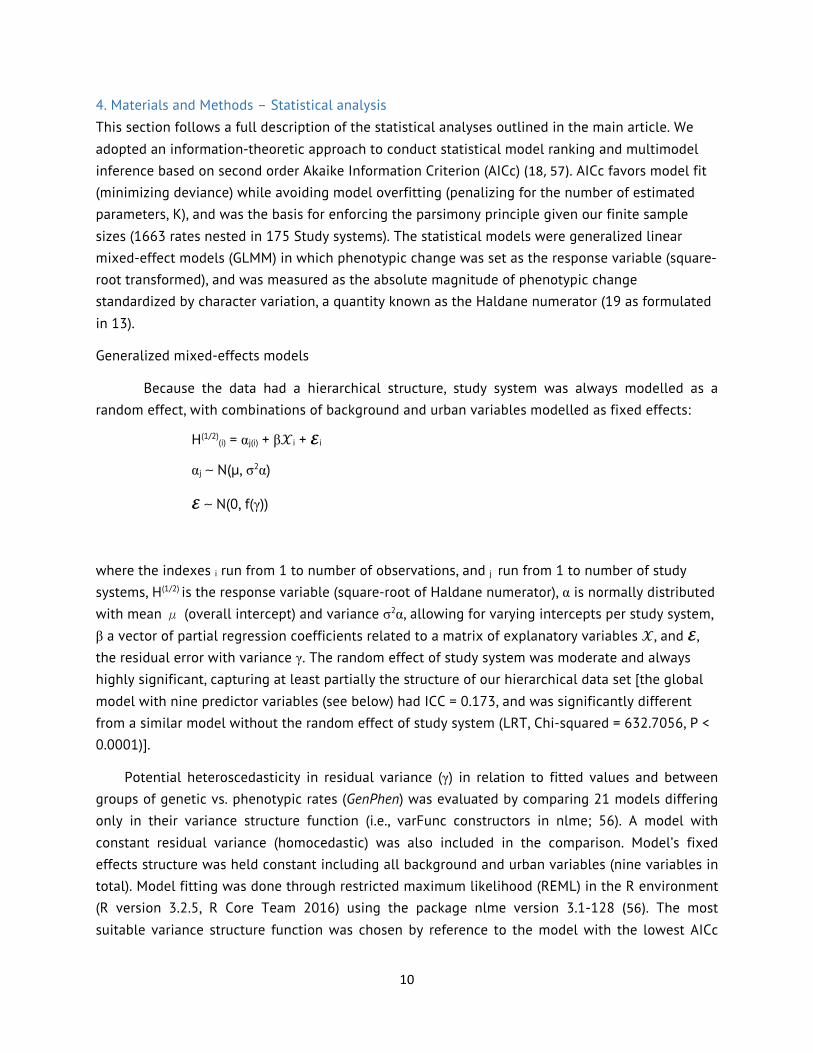
4. Materials and Methods – Statistical analysis This section follows a full description of the statistical analyses outlined in the main article. We adopted an information-theoretic approach to conduct statistical model ranking and multimodel inference based on second order Akaike Information Criterion (AICc) (18,  57). AICc favors model fit (minimizing deviance) while avoiding model overfitting (penalizing for the number of estimated parameters, K), and was the basis for enforcing the parsimony principle given our finite sample sizes (1663 rates nested in 175 Study systems). The statistical models were generalized linear mixed-effect models (GLMM) in which phenotypic change was set as the response variable (square-root transformed), and was measured as the absolute magnitude of phenotypic change standardized by character variation, a quantity known as the Haldane numerator (19 as formulated in 13).

Generalized mixed-effects models

Because the data had a hierarchical structure, study system was always modelled as a random effect, with combinations of background and urban variables modelled as fixed effects:

H(1/2)(i) = αj(i) + β𝒳i + 𝓔i

αj ∼ N(µ, σ2α)

𝓔 ∼ N(0, f(γ))

where the indexes i run from 1 to number of observations, and j run from 1 to number of study systems, H(1/2) is the response variable (square-root of Haldane numerator), α is normally distributed with mean μ (overall intercept) and variance σ2α, allowing for varying intercepts per study system, β a vector of partial regression coefficients related to a matrix of explanatory variables 𝒳, and 𝓔, the residual error with variance γ. The random effect of study system was moderate and always highly significant, capturing at least partially the structure of our hierarchical data set [the global model with nine predictor variables (see below) had ICC = 0.173, and was significantly different from a similar model without the random effect of study system (LRT, Chi-squared = 632.7056, P < 0.0001)].

Potential heteroscedasticity in residual variance (γ) in relation to fitted values and between groups of genetic vs. phenotypic rates (GenPhen) was evaluated by comparing 21 models differing only in their variance structure function (i.e., varFunc constructors in nlme; 56). A model with constant residual variance (homocedastic) was also included in the comparison. Model’s fixed effects structure was held constant including all background and urban variables (nine variables in total). Model fitting was done through restricted maximum likelihood (REML) in the R environment (R version 3.2.5, R Core Team 2016) using the package nlme version 3.1-128 (56). The most suitable variance structure function was chosen by reference to the model with the lowest AICc

11    

value, which was 2.05 lower than the second-best model. The selected model had the following residual variance structure:

γ = v * (C + |fitted|P)2

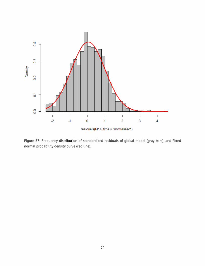
where v is a term of the estimated residual variance (0.1494), C is a constant by stratum (0.3233 for genetic; 0.1249 for phenotypic), and P an exponent of absolute fitted values by stratum (2.0754 for genetic; 1.2376 for phenotypic). Hence, the modelled residual variance increased exponentially with fitted values, and slightly more so in genetic than phenotypic rates (Fig. S5). This heteroscedastic model significantly enhanced model fit compared to a homoscedastic model (LRT, Chi-squared = 302.3283, P < 0.0001). A visual inspection of standardized residuals plotted against fitted values showed little pattern (unlike the homoscedastic model), and the distribution of residuals was nearly normal (Figures S6-S7). All subsequent GLMMs used the selected variance structure function for modeling residual variance (58).

Multimodel inference

Multimodel inference offers a means to tap into information contained in a model set while weighing model uncertainty. It is especially suited for exploratory data analyses, like ours, that are constrained by lack of knowledge, small sample size, high dimensionality of predictor variables, and high variability (18). We used exploratory multimodel inference to assess the relative importance of predictor variables (urban or not) for phenotypic change, and to make predictions about contrasting urban-related scenarios that considered information contained in all models at large.

From 3 background plus 6 urban variables, we combined 9 predictor variables to form 29 = 512 models, including a null model (intercept only), and excluding interactions. The variable anthropogenic context (anthropogenic associated to higher phenotypic change; 15) was excluded because it was correlated with, and confounds the effect of, urban disturbance (Supporting Information: 3. Gauging the urban signature beyond the anthropogenic context). Some of the retained explanatory variables were correlated to a lesser extent producing variance inflation factors generally (93%) below 2.5 (max = 2.7), which is considered below the threshold to remove collinear variables (58). Consequently, all partial regression coefficients of the global model were below 0.62, which reinforced our decision to retain all 9 predictor variables in further analyses.

All models, which also contained the random effect of Study system and the residual variance structure function previously selected, were fitted through maximum likelihood (ML) in the R package nlme (56). Models were ranked according to decreasing values of AICc (57), and further evaluated using standard methods after re-fitting through REML estimation (58).

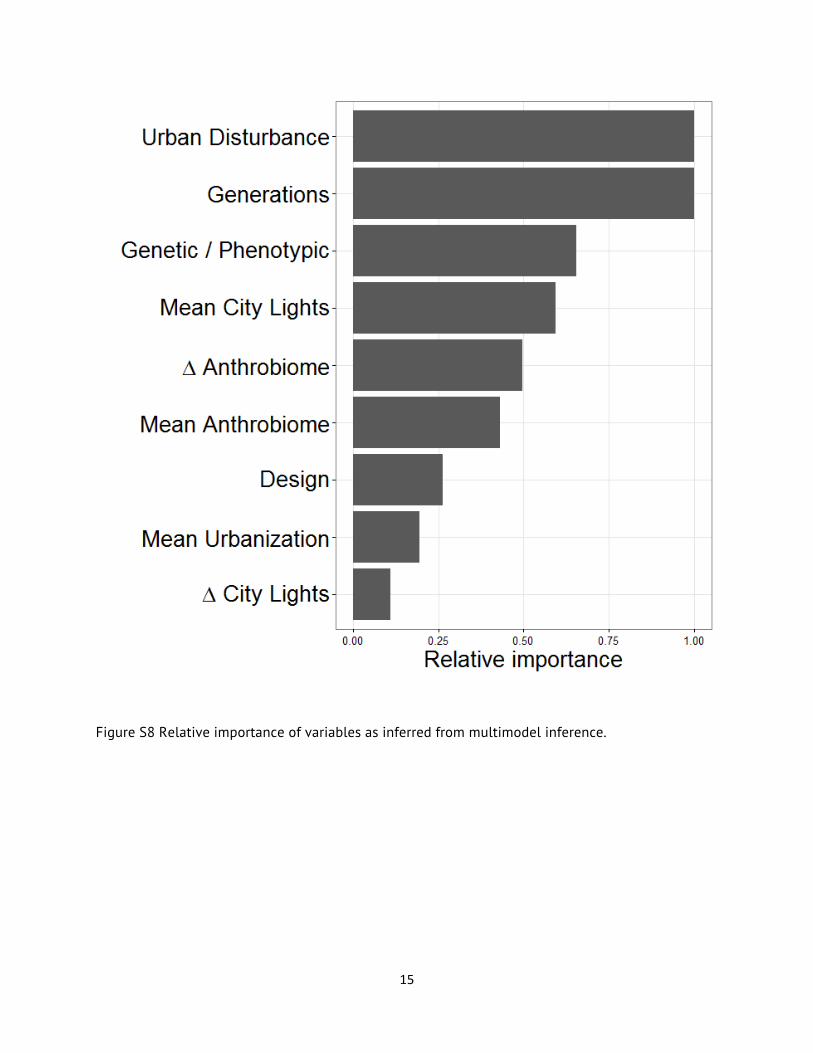
Predictor variable relative importance was calculated by the sum of the Akaike weights of all models containing a particular predictor variable. Urban disturbance variable was top-ranked, matched by log(Generations) (Figure S8), which, once again supports the importance of this variable in our analyses. Model-averaged partial regression coefficients (see main article) were Akaike-

12    

weighted averages of coefficients from all models containing a particular term (18). These coefficients allowed the illustration of effect sizes in terms of expected response (predictions) under particular scenarios (Table 1 and Figure 3, main article). For example, consistent with estimated variable relative importance, the range of predictions from different Urban Disturbance categories was higher than that of expected responses from varying background variables (Figure S9). Model ranking and inference was conducted in the R package MuMin v1.15.6 (55).

Figure S5: Selected model variance structure function. The expected residual variance increased exponentially with fitted values, and more so in genetic studies.

13    

Figure S6: Standardized residual plots of (top) homoscedastic global model, and (bottom) of global model bearing the selected heteroscedastic residual variance structure function.

14    

Figure S7: Frequency distribution of standardized residuals of global model (gray bars), and fitted normal probability density curve (red line).

15    

Figure S8 Relative importance of variables as inferred from multimodel inference.

16    

Figure S9 Multi-model predictions illustrating effect sizes, and distribution of observed phenotypic changes with respect to background variables: number of generations, study design (allochronic or synchronic), and genetic basis (genetic or phenotypic). Urban Disturbance (U. Disturbance) categories (symbols), and multi-model predictions for selected Urban Disturbance categories (regression lines and 95% confidence intervals) illustrate the gamut of expected effect sizes. The categories selected for display represent the range of expected effects due to Urban Disturbance (Table 1 and Figure 1, main article). Note the heterogeneous representation of predictor variable's categories in the data, and the relatively high effect sizes of Urban Disturbance compared to those of background variables, consistent with estimated variable relative importance (Fig S8). [For prediction, independent variables modeled but not shown were held statistically constant at mean values (continuous variables) or reference values (categorical variables). Data points where jittered horizontally to minimize superposition in the x-axis, hence the displayed number of generations is approximate.]

17    

References

1.     Post  DM,  Palkovacs  EP  (2009)  Eco-­‐evolutionary  feedbacks  in  community  and  ecosystem  ecology:  interactions  between  the  ecological  theatre  and  the  evolutionary  play.  Philos  Trans  R  Soc  Lond  B  Biol  Sci  364(1523):1629–1640.  

2.     Pimentel  D  (1961)  Animal  Population  Regulation  by  the  Genetic  Feed-­‐Back  Mechanism.  Am  Nat  95(881):65–79.  

3.     Schoener  TW  (2011)  The  Newest  Synthesis:  Understanding  the  Interplay  of  Evolutionary  and  Ecological  Dynamics.  Science  331(6016):426–429.  

4.     Matthews  B,  et  al.  (2011)  Toward  an  integration  of  evolutionary  biology  and  ecosystem  science.  Ecol  Lett  14(7):690–701.  

5.     Palkovacs  EP,  Kinnison  MT,  Correa  C,  Dalton  CM,  Hendry  AP  (2012)  Fates  beyond  traits:  ecological  consequences  of  human-­‐induced  trait  change.  Evol  Appl  5(2):183–191.  

6.     Alberti  M  (2015)  Eco-­‐evolutionary  dynamics  in  an  urbanizing  planet.  Trends  Ecol  Evolut  30(2):114–126.  

7.     United  Nations,  Department  of  Economic  and  Social  Affairs,  Population  Division  (2014)  World  urbanization  prospects:  the  2014  revision :  highlights  (ST/ESA/SER.A/352)  (New  York).  

8.     Seto  KC,  Gueneralp  B,  Hutyra  LR  (2012)  Global  forecasts  of  urban  expansion  to  2030  and  direct  impacts  on  biodiversity  and  carbon  pools.  PNAS  109(40):16083–16088.  

9.     Liu  J,  et  al.  (2013)  Framing  Sustainability  in  a  Telecoupled  World.  Ecol  Soc  18(2):26.  

10.     Marzluff  JM,  Angell  T  (2005)  Cultural  Coevolution:  How  the  Human  Bond  with  Crows  and  Ravens  Extends  Theory  and  Raises  New  Questions.  Journal  of  Ecological  Anthropology  9(1):69.  

11.     Hasselman  DJ,  et  al.  (2014)  Human  disturbance  causes  the  formation  of  a  hybrid  swarm  between  two  naturally  sympatric  fish  species.  Mol  Ecol  23(5):1137–1152.  

12.     Partecke  J  (2013)  Mechanisms  of  phenotypic  responses  following  colonization  of  urban  areas:  from  plastic  to  genetic  adaptation.  Avian  Urban  Ecology:  Behavioural  and  Physiological  Adaptations,  eds  Gil  D,  Brumm  H  (Oxford  University  Press,  Oxford,  UK),  p  131.  

13.     Hendry  AP,  Kinnison  MT  (1999)  Perspective:  The  pace  of  modern  life:  Measuring  rates  of  contemporary  microevolution.  Evolution  53(6):1637–1653.  

14.     Kinnison  MT,  Hendry  AP  (2001)  The  pace  of  modern  life  II:  from  rates  of  contemporary  microevolution  to  pattern  and  process.  Genetica  112:145–164.  

15.     Hendry  AP,  Farrugia  TJ,  Kinnison  MT  (2008)  Human  influences  on  rates  of  phenotypic  change  in  wild  animal  populations.  Molec  Ecol  17(1):20–29.  

18    

16.     Crispo  E,  et  al.  (2010)  The  evolution  of  phenotypic  plasticity  in  response  to  anthropogenic  disturbance.  Evol  Ecol  Res  12(1):47–66.  

17.     Gotanda  KM,  Correa  C,  Turcotte  MM,  Rolshausen  G,  Hendry  AP  (2015)  Linking  macrotrends  and  microrates:  Re-­‐evaluating  microevolutionary  support  for  Cope’s  rule.  Evolution  69(5):1345–1354.  

18.     Anderson  DR  (2008)  Model  Based  Inference  in  the  Life  Sciences:  A  Primer  on  Evidence  (Springer,  New  York ;  London).  1st  ed.  2008  edition.  

19.     Haldane  J  (1949)  Suggestions  as  to  Quantitative  Measurement  of  Rates  of  Evolution.  Evolution  3(1):51–56.  

20.     Nosil  P,  Harmon  LJ,  Seehausen  O  (2009)  Ecological  explanations  for  (incomplete)  speciation.  Trends  Ecol  Evol  24(3):145–156.  

21.     Winkel  W,  Hudde  H  (1997)  Long-­‐Term  Trends  in  Reproductive  Traits  of  Tits  (Parus  major,  P.  caeruleus)  and  Pied  Flycatchers  Ficedula  hypoleuca.  J  Avian  Biol  28(2):187–190.  

22.     Mittelbach  GG,  et  al.  (2001)  What  is  the  observed  relationship  between  species  richness  and  productivity?  Ecology  82(9):2381–2396.  

23.     Faeth  SH,  Warren  PS,  Shochat  E,  Marussich  WA  (2005)  Trophic  dynamics  in  urban  communities.  Bioscience  55(5):399–407.  

24.     McDonnell  M,  Hahs  A  (2008)  The  use  of  gradient  analysis  studies  in  advancing  our  understanding  of  the  ecology  of  urbanizing  landscapes:  current  status  and  future  directions.  Landscape  Ecol  23(10):1143–1155.  

25.     Marzluff  JM  (2005)  Island  biogeography  for  an  urbanizing  world:  how  extinction  and  colonization  may  determine  biological  diversity  in  human-­‐dominated  landscapes.  Urban  Ecosyst  8(2):157–177.  

26.     Pickett  STA,  et  al.  (2016)  Dynamic  heterogeneity:  a  framework  to  promote  ecological  integration  and  hypothesis  generation  in  urban  systems.  Urban  Ecosyst:1–14.  

27.     Aronson  MFJ,  et  al.  (2014)  A  global  analysis  of  the  impacts  of  urbanization  on  bird  and  plant  diversity  reveals  key  anthropogenic  drivers.  Proc  R  Soc  B  281(1780):20133330.  

28.     Groffman  PM,  et  al.  (2014)  Ecological  homogenization  of  urban  USA.  Front  Ecol  Environ  12(1):74–81.  

29.     Rebele  F  (1994)  Urban  Ecology  and  Special  Features  of  Urban  Ecosystems.  Global  Ecol  Biogeogr  4(6):173–187.  

30.     Shochat  E,  Warren  PS,  Faeth  SH,  McIntyre  NE,  Hope  D  (2006)  From  patterns  to  emerging  processes  in  mechanistic  urban  ecology.  Trends  Ecol  Evol  21(4):186–191.  

31.     Pickett  STA,  Wu  J,  Cadenasso  ML  (1999)  Patch  Dynamics  and  the  Ecology  of  Disturbed  Ground:  A  Framework  for  Synthesis.  Ecosystems  of  Disturbed  Ground,  ed  Walker  LR  (Elsevier  Science,  Amsterdam).  

19    

32.     Cardinale  BJ,  Hillebrand  H,  Charles  DF  (2006)  Geographic  patterns  of  diversity  in  streams  are  predicted  by  a  multivariate  model  of  disturbance  and  productivity.  J  Ecol  94(3):609–618.  

33.     Kille  P,  et  al.  (2013)  DNA  sequence  variation  and  methylation  in  an  arsenic  tolerant  earthworm  population.  Soil  Biol  Biochem  57:524–532.  

34.     Shenoy  K,  Crowley  PH  (2011)  Endocrine  disruption  of  male  mating  signals:  ecological  and  evolutionary  implications.  Funct  Ecol  25(3):433–448.  

35.     Bettencourt  LMA  (2013)  The  Origins  of  Scaling  in  Cities.  Science  340(6139):1438–1441.  

36.     Clucas  B,  Marzluff  JM  (2012)  Attitudes  and  actions  toward  birds  in  urban  areas:  Human  cultural  differences  influence  bird  behavior.  Auk  129(1):8–16.  

37.     Carroll  SP,  et  al.  (2014)  Applying  evolutionary  biology  to  address  global  challenges.  Science  346(6207):1245993.  

38.     Chislock  MF,  Sarnelle  O,  Jernigan  LM,  Wilson  AE  (2013)  Do  high  concentrations  of  microcystin  prevent  Daphnia  control  of  phytoplankton?  Water  Research  47(6):1961–1970.  

39.     Gluckman  PD,  Low  FM,  Buklijas  T,  Hanson  MA,  Beedle  AS  (2011)  How  evolutionary  principles  improve  the  understanding  of  human  health  and  disease.  Evol  Appl  4(2):249–263.  

40.     Thrall  PH,  et  al.  (2011)  Evolution  in  agriculture:  the  application  of  evolutionary  approaches  to  the  management  of  biotic  interactions  in  agro-­‐ecosystems.  Evolutionary  Applications  4(2):200–215.  

41.     McMahon  RF  (1976)  Effluent-­‐induced  interpopulation  variation  in  the  thermal  tolerance  of  Physa  virgata  gould.  Comp  Biochem  Physiol  A  Comp  Physiol  55(1):23–28.  

42.     Al-­‐Hiyaly  SAK,  McNeilly  T,  Bradshaw  AD  (1990)  The  effect  of  zinc  contamination  from  electricity  pylons.  Contrasting  patterns  of  evolution  in  five  grass  species.  New  Phytol  114(2):183–190.  

43.     Haugen  TO,  Aass  P,  Stenseth  NC,  Vøllestad  LA  (2008)  Changes  in  selection  and  evolutionary  responses  in  migratory  brown  trout  following  the  construction  of  a  fish  ladder.  Evol  Appl  1(2):319–335.  

44.     Trussell  GC,  Smith  LD  (2000)  Induced  defenses  in  response  to  an  invading  crab  predator:  An  explanation  of  historical  and  geographic  phenotypic  change.  P  Natl  Acad  Sci-­‐Biol  97(5):2123–2127.  

45.     McGraw  JB  (2001)  Evidence  for  decline  in  stature  of  American  ginseng  plants  from  herbarium  specimens.  Biol  Conserv  98(1):25–32.  

46.     Blumstein  DT,  Daniel  JC  (2003)  Foraging  behavior  of  three  Tasmanian  macropodid  marsupials  in  response  to  present  and  historical  predation  threat.  Ecography  26(5):585–594.  

47.     Franks  SJ,  Sim  S,  Weis  AE  (2007)  Rapid  evolution  of  flowering  time  by  an  annual  plant  in  response  to  a  climate  fluctuation.  PNAS  104(4):1278–1282.  

20    

48.     Jenni  L,  Kéry  M  (2003)  Timing  of  autumn  bird  migration  under  climate  change:  advances  in  long–distance  migrants,  delays  in  short–distance  migrants.  P  Roy  Soc  Lond  B  Bio  270(1523):1467–1471.  

49.     Odling-­‐Smee  FJ,  Laland  KN,  Feldman  MW  (2003)  Niche  construction:  the  neglected  process  in  evolution  (Princeton  University  Press,  Princeton).  

50.     Bouma  TJ,  Vries  MBD,  Herman  PMJ  (2010)  Comparing  ecosystem  engineering  efficiency  of  two  plant  species  with  contrasting  growth  strategies.  Ecology  91(9):2696–2704.  

51.     Marzluff  JM  (2012)  Urban  Evolutionary  Ecology.  Urban  Bird  Ecology  and  Conservation,  eds  Lepczyk  CA,  Warren  PS  (University  of  California  Press),  pp  286–308.  

52.     Zhou  Y,  et  al.  (2015)  A  global  map  of  urban  extent  from  nightlights.  Environ  Res  Lett  10(5):054011.  

53.     Zhou  Y,  et  al.  (2014)  A  cluster-­‐based  method  to  map  urban  area  from  DMSP/OLS  nightlights.  Remote  Sensing  of  Environment  147:173–185.  

54.     Ellis  EC,  Ramankutty  N  (2008)  Putting  people  in  the  map:  anthropogenic  biomes  of  the  world.  Front  Ecol  Environ  6(8):439–447.  

55.     Barton  K  (2016)  Package  “MuMIn:”  Multi-­‐Model  Inference.  R  package  version  1.15.6.  Available  at:  https://cran.r-­‐project.org/web/packages/MuMIn/MuMIn.pdf  [Accessed  August  9,  2016].  

56.     Pinheiro  J,  Bates  D,  DebRoy  S,  Heisterkamp  S,  Van  Willigen  B  (2016)  Package  “nlme”  Available  at:  https://cran.r-­‐project.org/web/packages/nlme/nlme.pdf  [Accessed  August  5,  2016].  

57.     Burnham  KP,  Anderson  DR  (2003)  Model  Selection  and  Multimodel  Inference:  A  Practical  Information-­‐Theoretic  Approach  (Springer,  New  York).  2nd  edition.  

58.     Zuur  AF  ed.  (2009)  Mixed  effects  models  and  extensions  in  ecology  with  R  (Springer,  New  York,  NY).