! "#

Heshmati, A.

Almas Heshmati

MTT Economic Research Luutnantintie 13

FIN-00410 Helsinki, Finland Phone: +358-9-56086213 Fax: +358-9-56086264

E-mail: Almas.Heshmati@mtt.fi

July 20, 2004

This paper is a review of recent developments of parametric and non-parametric approaches to decompose inequality by subgroups, income sources, causal factors and other unit characteristics. Different methods of decomposing changes in poverty into growth, redistribution, poverty standard and residual components are described. In parametric approaches the dynamics of income accounting for transitory and permanent changes in individual and household earnings conditional of various covariates are also reviewed. Statistical inferences for inequality measurement including delta and bootstrapping and other methods to provide estimates of the sampling distribution are presented. These issues are important in the design of policy measures and expectations about their impacts on earnings inequality and poverty reductions.

Income inequality, poverty, decomposition, parametric, non-parametric, Gini index

!"#"$!%"&'() C10; D31; I32; N30.

'**%$"%!%"&Heshmati, A. (2004)+A Review of Decomposition of Income Inequality. MTT Economic Research, Agrifood Research Finland. Discussion Papers 2004/8.

∗ An earlier version of this paper was completed while I was working at the World Institute for Development Economic Research, UNU/WIDER.

1

,+

There is an ongoing and increasing interest in measuring and understanding the level, causes and development of income inequality. The 1990s signified a shift in research previously focused on economic growth, the identification of the determinants of economic growth and convergence in GDP per capita across countries to analysis of distribution of income, its development over time and identification of factors determining the distribution of income. This shift in focus is specifically from the issues of convergence or divergence of per capita incomes to the long-term equalisation or polarisation of incomes across regions and countries.1 This shift is not only a reflection of technological change and raised human capacity to create growth and wealth, but also due to awareness of the growing disparity and importance of redistribution and poverty reduction. The growing disparity calls for analysis of various aspects of income inequality including its measurement, decomposition and causal factors.

Income inequality refers to the inequality of the distribution of individuals, household or some per capita measure of income. Lorenz Curve is used for analysing the size distribution of income and wealth and measures of inequality and poverty. It plots the cumulative share of total income against the cumulative proportion of income receiving units. The divergence of a Lorenz curve for perfect equality and the Lorenz curve for a given income distribution is measured by some index of inequality. The most widely used index of inequality is the Gini coefficient (for reviews of the notion and analysis of inequality see Subramanian 1997 and Cowell 2000). There are two parametric approaches to estimate the Lorenz curve (Ryu and Slottje, 1999). In the first approach one assumes a hypothetical statistical distribution for income distribution and in the second approach, a specific functional form is fit to the Lorenz curve directly (Chotikapanich and Griffiths 2002). An important drawback of the traditional models of the Lorenz curve is a lack of satisfactory fit over the entire range of a given income distribution. Ogwang and Rao (2000) proposed two hybrids Lorenz curves by combination of traditional models. The estimated Lorenz curve is sensitive to errors in survey data. The robustness properties of inequality and poverty measures assuming contaminated data with illustrations are considered in Cowell and Victoroa-Feser (1996a and 1996b). Hasegawa and Kozumi (2003) propose using Bayesian non-parametric analysis and present a method for removing the contaminated observations.

Several inequality indices can be derived from the Lorenz diagram. The Lorenz Curve construction also gives us a rough but standard measure (Gini coefficient) of the amount of inequality in the income distribution. The index lies in the interval 0 (perfect equality) and 1 (perfect inequality). Among the other notable measures of inequality are: the range, the variance, the squared coefficient of variation, the variance of log incomes, the absolute and relative mean deviations, and Theil’s two inequality indices.

1 For a selection of studies of growth and convergence in per capita incomes see: Barro (1991), Barro and Sala-i-Martin (1995), Islam (1995), Lee, Pesaran and Smith (1997), Mankiew, Romer and Weil (1992), and Quah (1996). Quah (2002), Ravallion (2003), Sala-i-Martin (2002a, 2002b), and Solimano (2001) analysed convergence in income inequality, while Acemoglu and Ventura (2002), Atkinson (1997, 1999), Bourguignon and Morrisson (2002), Cornia (1999), Gottschalk and Smeeding (1997) and Milanovic (2002) focus on the distribution of income. More recently Acemoglu (2002), Caminada and Goudswaard (2001), Cornia and Kiiski (2001), Gotthschalk and Smeeding (2000), Milanovic (2002), O’Rourke (2001), Park (2001), Sala-i-Martin (2002b) and Schultz (1998) studied trends in income inequality.

2

The indices have different properties that can be used in their ranking, relevance and performance evaluation. There are three basic properties that one would expect that the above indices of inequality to satisfy: mean or scale independence, population size independence and the Pigou-Dalton condition. The Gini coefficient, the squared coefficient of variation and the two Theil’s measures satisfy each of the three properties, while the relative and absolute mean difference and the range measures satisfy only the first two conditions. The variance measure violates the mean independence property. For more details on the properties of the different indices of inequality see Anand (1997). A generalization of the Gini coefficient, called the extended Gini coefficient, was introduced by Yitzhaki (1983). The new index accommodates differing aversions to inequality. Empirical estimation of the extended index has been limited to the covariance formula suggested by Lerman and Yitzhaki (1989). Chotikapanich and Griffiths (2001) suggest an alternative estimator, obtained by approximating the Lorenz curve by a series of linear segments.

Inequality can have many dimensions. Economists are concerned specifically with the economics or monetarily measurable dimension related to individual or household income and consumption. However, this is just one perspective and inequality can be linked to inequality in skills, education, opportunities, happiness, health, life expectancy, welfare, assets and social mobility. The effects of inequality in non-income factors on earnings can be summarised variously. Inequality in education explains a minor fraction of differences in cross-country earnings inequality. The impact decreases by the level of education and depends on the economic development and skill-intensive nature of production technologies. It also negatively affects the investment rate and growth rate of income. There is no direct link from income inequality to ill health measured as mortality, but a range of mechanism and social arrangements indicate the presence of an indirect link. Unlike in the case of income inequality, within country health inequality is a dominating source of inequality. The non-income dimension of inequality is beyond the scope of this paper. Heshmati (2004) reviews the recent advances in the measurement of inequality and gives attention to the interrelationship between income inequality and the non-income inequality dimensions.

Different methods have been developed to decompose inequality (Pyatt 1976; Shorrocks 1980, 1982 and 1984; Fields 2000; Morduch and Sicular 2002), and changes in poverty (Kakwani and Subbaro 1990; Jian and Tandulkat 1990; Datt and Ravallion 1992; and Shorrocks and Kolenikov 2001). Inequality is decomposed by sub-groups, income sources, causal factors and by other sociodemographic characteristics. Inequality can also be decomposed at different levels of aggregation. At the national level it can be decomposed into within-subgroup and between-subgroup components. In a similar way at the international level it can be decomposed into within-country and between-country components. A decomposition of inequality and changes in poverty are important in the design of policy measures, their expected effects and in evaluation of the impacts of inequality and redistributive policies on welfare among regions, sub-groups and sectors. Inequality can also at the micro level be decomposed parametrically into permanent and transitory components of earnings (e.g. Geweke and Keane 2000; Zandvakili 2002; and Moffitt and Gottschalk 2002). The main benefits of parametric approaches are that changes are conditional on various heterogeneity attributes not all captured by the growth and redistribution components. Furthermore confidence intervals for disaggregated contributions to the inequality index can be constructed.

3

Having discussed the different dimensions and measurement of inequality and listed the indices of income inequality derived from the Lorenz curve this paper has a major contribution to the inequality literature. First, it provides the current state of knowledge on recent developments in inequality decomposition by population subgroups, income sources, inequality causal factors and other sociodemographic characteristics. Second, different methods of decomposing changes in poverty into growth, redistribution, poverty standard and residual components are discussed as well. Third, in parametric decomposition approaches the dynamics of income accounting for transitory and permanent changes in individual and household earnings conditional of various covariates are also reviewed. Finally, statistical inferences for inequality measurement including delta and bootstrapping methods to provide estimates of the sampling distribution and jackknife, as well as regression methods to report Gini standard errors and normalised stochastic dominance to rank inequality in case when the distribution of income has different means are discussed.

Rest of the paper is organised as follows. The next Section introduces the readers to the origin of the modern income inequality decomposition. Section 3 is a review of the development of decomposition of changes in poverty into growth, redistribution and poverty standard components. In Section 4 changes in the distribution of income is decomposed and related to the sociodemographic characteristics of the population. Section 5 and 6 are on decomposition of inequality by causal factors and by sub-groups of the population. The adjustment process towards equilibrium income is also discussed. The regression-based inequality decomposition by income sources and confidence intervals for disaggregated contributions to the inequality index is discussed in Section 7. The transitory and permanent components of shocks to the earnings are distinguished in Section 8. Here the focus on the dynamics in individual earnings, sub-group heterogeneity and their policy implications. Section 9 and 10 are on the statistical inference for inequality measurement and inferences about the Gini index. The final Section summarises.

-+

The origin of the modern inequality decomposition literature is to be found in Shorrocks (1980, 1982 and 1984),2 where he examined decomposition of inequality by income sources such as earnings, investment income and transfer payments; by population subgroups like single persons, married couples, and families with children; or by subaggregates of observations which share common characteristics like age, household size, region, occupation, or some other attributes. He shows that a broad class of inequality measures can be decomposed into components reflecting only the size, mean and inequality value of each population subgroup or income source.

2 The current state of knowledge regarding the theory and application of inequality decomposition techniques in a spatial and regional context is reviewed by Shorrocks and Wan (2004). They emphasis that the time profile of the within and between-group components of inequality will add a dynamic dimension to the studies of spatial inequality decomposition. An examination of the linkage of between-group inequality to growth is more informative compared to analysis of sigma convergence. Attention should be paid to the factors contributing to spatial inequality, persistency in spatial differences and the influence of migration.

4

In decomposing income inequality Shorrocks (1983) examines the relative influence of income components and evaluates the performance of different decomposition rules using US data. The method can be based on the Gini coefficient written as:

(1) ∑=

⎟⎠⎞⎜

⎝⎛ +−=

12 2

12)(

µ

where ∑ ==

1 is the sum of these income components. The inequality

decomposition rules for factor components can be generated for inequality measures of the form:

(2) ∑∑∑== =

==

11 1

)()(

where

is a contribution of factor to overall income inequality,

is the weight

attached to individual income component ,

. The proportional factor contribution

in aggregate income is expressed as:

(3) )(/),cov()(/ 2

σ==

with ∑ = 1. Empirical results are based on panel data consisting of 2755 households

observed for 1967-76 obtained from the PSID. Analyses of the distribution of net family incomes result in identification of ten factor components.3 There is a fair but far from identical degree of correspondence between the inequality contribution and income share of each factor component. Labour income of head (of household) and head and spouse direct taxes are the main positive and negative factors respectively, contributing to the inequality of total net family incomes in the US. Cowell and Jenkins (1995) apply different decomposition techniques and investigate the quantitative importance of principal population (sex, race and age of head) and labour market (employment status) characteristics in explaining inequality using PSID data. Results are robust under alternative methods of decomposition and the within-group component dominates. Jenkins (1995) applied inequality decomposition methods to UK data, and the results indicate that these decompositions generate different results when used with different inequality indices, when the indices are sensitive to extreme income observations. This, together with the increased interest for and the importance of inequality decomposition, has resulted in alternative decomposition approaches being developed.

The effects of growth on income poverty have been studied by accounting for changes in the distribution of income. Income poverty ),,( µ is expressed in terms of poverty line )( , mean income level )(µ and the relative distribution of income )( .

3 Factors contributing to inequality of total net family incomes are: taxable income of head of household and spouse ((i) labour income of head (ii) spouse and (iii) income from capital), transfer income of head and spouse ((iv) welfare benefits (v) pensions and (vi) other transfer income), income of other family members ((vii) taxable income (viii) transfer income), direct taxes ((ix) head and spouse (x) other family members).

5

The Lorenz curve represents the structure of relative income inequalities. Assuming the poverty line is fixed at a given level, income poverty is given by ),( µ . The total change in poverty )( ∆ is then decomposed into two components. The first component is the growth component due to changes in the mean income while holding the Lorenz curve constant at some reference level, and the second a redistribution component due to changes in the Lorenz curve while keeping the mean income constant at some reference level. There are a number of ways to decompose the total change in poverty. Kakwani and Subbaro’s (1990) decomposition approach is:

(4)

+=−+−=−=−=∆

),(),(),(),(),(),(

01110001

001101

µµµµµµ

where and,µ are mean income and the Lorenz curve characterizing the distribution of income. The subscripts 0 and 1 denote the two (consecutive or non-consecutive) initial and final periods of observation, and and are contributions from the growth and redistribution components. In analyzing the impact of economic growth on poverty in India, Kakwani and Subbaro measure separately the impacts of changes in average income and income inequality on poverty. They examine trends in the distribution and growth of consumption and assess their relative impacts on the poor and ultra poor, over the period 1972-83 and across the 15 major states of India.4 Results suggest that the beneficial effect of growth on the incidence of poverty during 1973-77 was outweighed by the adverse movements in the inequality of consumption. However, during 1977-83 average consumption grew slowly and consumption inequality fell in many states mainly reducing the incidence of ultra poor poverty. States differ in needs, capacities, social policy, intervention programmes and performance.

For the same decomposition purpose Jain and Tendulkar (1990) proposed:

(5) ),(),(),(),(),(),(

00101011

001101

µµµµµµ

−+−=−=−=∆

.

The two decompositions differ by the way the two growth and redistribution components are computed; differences in the reference point: base year versus final year. In the choice of base year in multiple time period comparisons one might take the quality of the data point and its relevance into consideration. Datt and Ravallion (1992) found the above decompositions of poverty changes as being time path dependent, arising through and dependent on the choice of reference levels. To make the changes path independent they proposed:

(6)

+−+−=−=−=∆

),(),(),(),(),(),(

00100001

001101

µµµµµµ

where is an extra residual component appended to the (8). The residual exists whenever the poverty measure is not additively separable between andµ . It is the difference between the growth (redistribution) components evaluated at the terminal and

4 The poverty line defined by the Indian Planning Commission in 1979. It corresponds to the per capita total expenditure required to attain some basic nutritional norm: daily intake of 2400 calories in rural area, 1973-74 prices. Ultra poor is defined as based on a poverty line equivalent of 80 per cent of the poor poverty line.

6

initial Lorenz curves (mean incomes), respectively. The residual does not vanish unless andµ remain unchanged over the decomposition period, nor apportioned between the

two components. The two growth and redistribution components differ by the base year or reference level chosen as a benchmark. This decomposition can be applied to multiple periods where a fixed reference point, like the first period, is required for sub-period additively to be satisfied.

In their application of the decomposition method Datt and Ravallion use three measures of poverty (headcount, poverty gap and Foster-Greer-Thorbecke – FTG) where the Lorenz curve is parametrized as beta and general quadratic functional forms. The poverty measure and their decompositions are estimated for rural and urban India during 1977-78, 1983, 1986-87, and 1988 and for Brazil 1981-88. In addition to the data problem, the method is found to have a number of limitations. Results indicate the presence of heterogeneity both over time and across the two countries: the method allows quantification of the relative importance to the poor of the differences in mean and inequality. However it can not identify alternative growth processes with better distributional implications to reduce poverty more effectively, nor whether a shift in distribution or mean is politically or economically attainable. The method was used by Assadzadeh and Paul (2003) to show how growth and redistribution policies affected poverty measured as headcount, poverty gap and FGT(2) in Iran during 1983, 1988 and 1993. Results show that the growth component affected negatively the rural but positively the urban sector while the redistribution component was positive implying that deterioration of inequality had contributed to the worsening of poverty in Iran.

Dhongde (2002) rewrites the total change in poverty described above decomposed into its components as:

(7) [ ] [ ] 2/),(),(),(),(

2/),(),(),(),(),(),(

00100111

10110001

001101

µµµµµµµµ

µµ

−+−+−+−=

−=−=∆

where the two growth and distribution components are averaged. The advantage of this method is that with the presence of time dependency the averaging procedure achieves path independence in the decomposition. Another advantage is that there is no residual or unexplained part of the total change. This of course is dependent on the assumption that the total change in poverty can be decomposed into growth and redistribution components. If all income poverty changes can not be explained by these two components the resulting residuals are allocated to the two components biasing the changes but leaving the total unchanged. The method is applied to data from 15 Indian states comparing changes in poverty from 1983/84 to 1993/94 and 1993/94 to 1999/2000. The poverty lines correspond to the per capita total expenditure required to attain some basic nutritional norm: daily intake of 2400 calories in rural and 2100 calories in urban areas, at 1973-74 prices (Kakwani and Subbaro, 1990). The results show that new sets of policies boost growth of per capita income leading to a decline in poverty. However, as previously observed by Kakwani and Subbaro the growth was accompanied by negative changes in the distribution of income and not in favour of the poor. The adverse impact was stronger in urban areas.

In a similar decomposition approach, but relaxing the assumption of fixed poverty line, Shorrocks and Kolenikov (2001) investigate how changes in mean income, inequality

7

and the poverty standard have affected the level of poverty in Russia. The total change in poverty defined as:

(8)

+−+−+−=

+++=−=−=∆

),,(),,(),,(),,(),,(),,(

),,(),,(

000100

000010000001

00011101

µµµµµµ

µµ

where and,µ are mean income, the Lorenz curve and the poverty rate characterizing the distribution of income. The subscripts 0 and 1 denote two periods of observation, and , , and are contributions from the growth, redistribution, poverty standard effects and the extra residual or overlapping components. Shorrocks and Kolenikov quantify the contributions of these factors to the year-by-year changes in the poverty rate and its development since 1985. Based on household data for 1985-99 rising inequality is identified as the principal cause of the high poverty rate in Russia. A decomposition analysis based on consecutive year-by-year changes has the advantages that it is not sensitive to random transitory shocks and less to measurement error in the data.

The recent development of inequality decomposition techniques is summarized as follows. It is possible to decompose inequality by income sources and population subgroups. The results are however sensitive to the choice of different inequality indices resulting in development of alternative decomposition approaches. Regression-based methods are used to estimate the relative contribution of different variables on aggregate inequality. Personal, family, human capital, regional and political variables explain emerging inequality. Another method is to construct the distribution of earnings or changes in poverty rate by assuming distributional characteristics with different time periods as the benchmark. The changes are then decomposed into various components and related to various determinants.

Cameron (2000) modified DiNardo . (1996) where the changes in the cumulative distribution functions, Lorenz curves and generalized Lorenz curves (GL) are decomposed. She examines the changes in the distribution of per capita income between 1984 and 1990 in Java and relates it to the ageing of the population, higher educational attainment, movement out of agriculture and changes in average income () within industries and age/education categories as:

(9) [ ]

+−=

−=−=∆),,,,,;(),,,,,;(

)()(

9084

908401

where , and , are the household head’s age, education and main source of income attributes, and , , and are distributional characteristics, the mean of per capita income in age/education categories, period and residuals. The advantage of this method is that it presents decompositions in terms of probability density functions rather than summary statistics such as the Gini coefficient. Ranking income distribution by the means of the GL ordering is a commonly used procedure in welfare economics. However, this approach ignores the needs identified by the non-income demographic characteristics of individuals like marital status, family size, etc. Atkinson and Bourguignon (1987) introduced the sequential GL rank ordering to more realistic cases

8

with heterogeneous income distribution where the population is partitioned into subgroups on the basis of needs. This ordering has a strong utilitarian support. Ok and Lambert (1999) in their evaluation of social welfare by sequential GL dominance outline an extension of the Atkinson–Bourguignon analysis, and show that the sequential GL ordering is supported by all increasing social welfare functions which record an increase in overall welfare when a welfare transfer is made from less needy to more needy subgroups.

Bourguignon, Fournier and Gurgand (2001) proposed a decomposition method where they parametrically construct a distribution at the terminal year with the initial year’s characteristics and compare the resulting distribution with the initial year distribution:

(10) ),,,(),,,(

),,,();;,(

'''''

λβελβελβε

λβε

−===

where is income of individual (household) in period ,

is the overall distribution

of household incomes, are observable sociodemographic characteristics,

ε are

unobservable characteristics,

β are a vector of prices and labour remuneration rates, λ

a vector of occupational choice behavioural parameters, ),,( '''' represent a

vector of price effects )( ' , participation effect )( '

and population effect )( '

computed as the difference between two dates 'and . It is to be noted that the wage model allows for parameter heterogeneity over time and across gender. In the estimation of the wage equation assuming fixed effects it is accounted for selection bias.

Bourguignon, Fournier and Gurgand (2001) applied the above decomposition method to examine the changes in the Taiwanese distribution of individual and household earnings between 1979 and 1994, to isolate the respective impacts of changes in the earnings structure, labour-force participation behaviour and sociodemographic (age, education, household size, etc.) structure of the population. Results indicate that various structural forces offset each other, and four phenomena were found to be important to the evolution of the distribution of individual earnings. These are: (i) changes in the wage structure due to increased returns to schooling and supply of educated workers which contributed to increased inequality, (ii) a drop in the variance of the effect of unobserved earnings, (iii) changes in participation and occupational choice behaviour that increased the share of middle-income earners, and (iv) changes in the sociodemographic structure of the population. The same phenomena affected the distribution of earnings of household units but somewhat different than that of individual units indicating significance of within household distribution of earnings.

To evaluate the pro-poor nature of changes in income inequality Jenkins and Van Kerm (2003) propose a decomposition that links changes in income inequality over time in the US (1981-93) and Germany (1985-99) to the extent to which income growth is pro-poor and to the extent of income reranking. Changes in the Lorenz curve is broken down into two parts: a reranking index measuring the relative-income-weighted average of changes in social weights and an index measuring the progressivity of income growth. Results show that in both countries income growth is pro-poor, reducing inequality; however the effect is offset by the disequalizing impact of changes in income ranking, and this is stronger in the US.

9

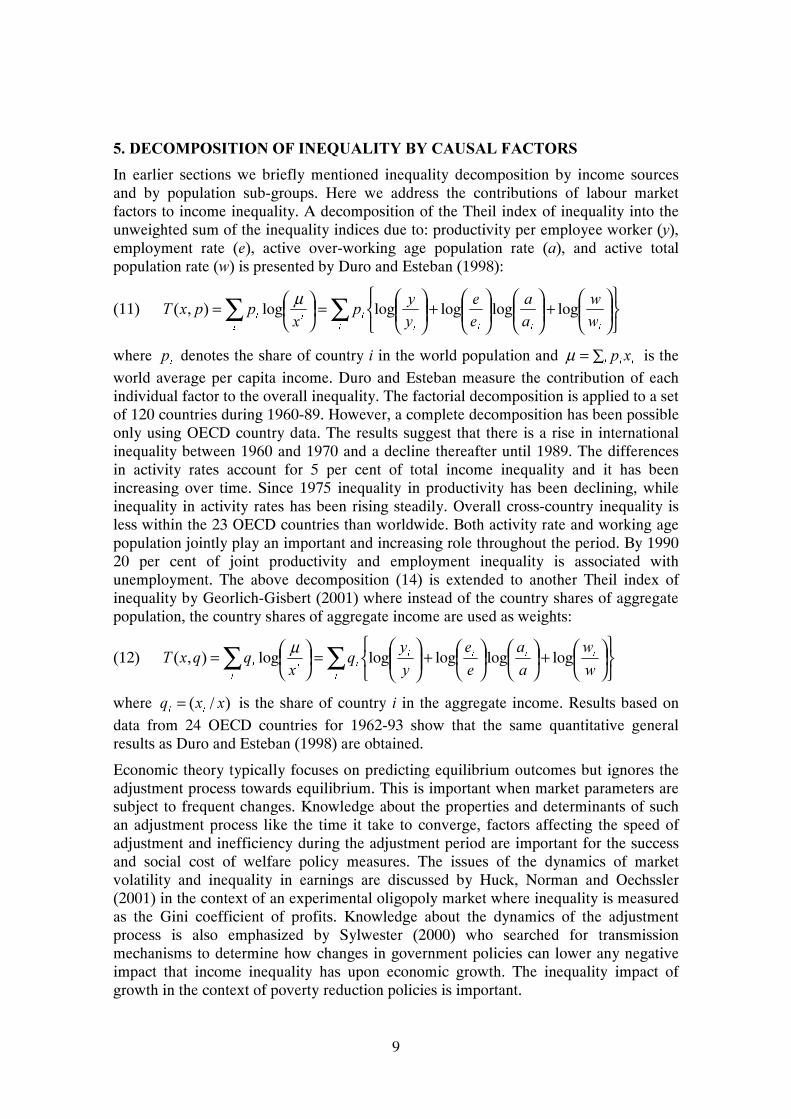
In earlier sections we briefly mentioned inequality decomposition by income sources and by population sub-groups. Here we address the contributions of labour market factors to income inequality. A decomposition of the Theil index of inequality into the unweighted sum of the inequality indices due to: productivity per employee worker (), employment rate (), active over-working age population rate (), and active total population rate () is presented by Duro and Esteban (1998):

(11) ∑∑⎭⎬⎫

⎩⎨⎧

⎟⎟⎠

⎞⎜⎜⎝

⎛+⎟⎟⎠

⎞⎜⎜⎝

⎛⎟⎟⎠

⎞⎜⎜⎝

⎛+⎟⎟⎠

⎞⎜⎜⎝

⎛=⎟

⎠⎞⎜

⎝⎛=

logloglogloglog),(µ

where

denotes the share of country in the world population and ∑= µ is the

world average per capita income. Duro and Esteban measure the contribution of each individual factor to the overall inequality. The factorial decomposition is applied to a set of 120 countries during 1960-89. However, a complete decomposition has been possible only using OECD country data. The results suggest that there is a rise in international inequality between 1960 and 1970 and a decline thereafter until 1989. The differences in activity rates account for 5 per cent of total income inequality and it has been increasing over time. Since 1975 inequality in productivity has been declining, while inequality in activity rates has been rising steadily. Overall cross-country inequality is less within the 23 OECD countries than worldwide. Both activity rate and working age population jointly play an important and increasing role throughout the period. By 1990 20 per cent of joint productivity and employment inequality is associated with unemployment. The above decomposition (14) is extended to another Theil index of inequality by Georlich-Gisbert (2001) where instead of the country shares of aggregate population, the country shares of aggregate income are used as weights:

(12) ∑∑⎭⎬⎫

⎩⎨⎧

⎟⎠⎞⎜

⎝⎛+⎟

⎠⎞⎜

⎝⎛⎟

⎠⎞⎜

⎝⎛+⎟⎟⎠

⎞⎜⎜⎝

⎛=⎟

⎠⎞⎜

⎝⎛=

logloglogloglog),(

µ

where )/(

= is the share of country in the aggregate income. Results based on

data from 24 OECD countries for 1962-93 show that the same quantitative general results as Duro and Esteban (1998) are obtained.

Economic theory typically focuses on predicting equilibrium outcomes but ignores the adjustment process towards equilibrium. This is important when market parameters are subject to frequent changes. Knowledge about the properties and determinants of such an adjustment process like the time it take to converge, factors affecting the speed of adjustment and inefficiency during the adjustment period are important for the success and social cost of welfare policy measures. The issues of the dynamics of market volatility and inequality in earnings are discussed by Huck, Norman and Oechssler (2001) in the context of an experimental oligopoly market where inequality is measured as the Gini coefficient of profits. Knowledge about the dynamics of the adjustment process is also emphasized by Sylwester (2000) who searched for transmission mechanisms to determine how changes in government policies can lower any negative impact that income inequality has upon economic growth. The inequality impact of growth in the context of poverty reduction policies is important.

10

In sum income distributions are heterogeneous, reflecting differences in the needs of subgroups of the population. In cross-country inequality decomposition the choice of population or income weights is important. The frequent changes in market parameters also require taking into account the adjustment process towards equilibrium income. Knowledge of the determinants, speed and social cost of policy measures is thus of great interest.

Yitzhaki (2002) decomposed the Gini coefficient to evaluate the impact of policy instruments on income inequality and the components of the Gini index. Society is divided into two groups: the poor with income below the poverty line , ≤ , and the rich with income above the poverty line, > . The overall Gini coefficient of income is thus composed:

(13)

++=

where and are population and income shares, and the superscripts , , , and denote the overall, poor, rich and between-groups. The inequality index is decomposed into inequality within poor and rich groups, and between the two groups. The latter can be further decomposed into a poverty gap, an affluence gap, and a poverty–affluence-lines gap component. The analysis is performed with family expenditure data from Romania for 1993. Results suggest that the dominant consideration in any poverty alleviation programme should be devoted to how much is transferred from the less needy to the poor, rather than how subsidies are allocated among the poor.

Income inequality measured for more disaggregated subgroups like single mothers, retired, disabled or by race, sex, age and marital status is important for redistributive policy analysis. Income inequality among female heads of household investigated by Zandvakili (1999) focuses on the factors that might have influenced earnings inequality using generalized entropy measures of inequality in both short- and long-term incomes over 1978-86 with PSID data. Income is measured as total family income adjusted for household size using equal weights given to each household member. Inequality decomposed by short- and long-term and income stability for overall sample and for sample decomposed by various household characteristics are reported by Zandvakili. The stability (mobility) index is calculated as:

(14) ∑

∑∑

−

==

)(

)/1log(

)(

)(*1

γγ

γ

µµ

where and denote household and periods, 1,0,1 −≠=γ determine the sensitivity to

different portions of the distribution of income, )(γ and )(

γµ∑ are long-term and

weighted average of short-term inequalities, ∑= )/(* is income share,

),.....,,( 21 = , and ),.....,,( 21

= income vectors at time . The stability

index, 10 ≤≤

, can be decomposed into between-group and a weighted average of

the within-group components,

+= , by replacing and with

11

and,, , respectively. The results show that short-term inequality has increased due to the existence of transitory components, while long-term inequality decreased in the early years. Race, in conjunction with education, is found to be the most influential factor explaining more than 30 per cent of the inequality. Age and marital status were also examined as possible contributors. Most movement occurs within each race group and cross group equalization is minimal.

Zandvakili and Mills (2001) used PSID data for 1981-91 to investigate the distributional consequences of changes in tax laws and transfer payments in the US. Income inequality is measured for both pretax/transfer and posttax/transfer definitions of household income. Using bootstrap methods confidence intervals are constructed for various Generalized Entropy measures of inequality and hypothesis tested. Using decomposable (within and between Theil 1 and Theil 2) measures of inequality the implications of type of tax scale are investigated. Results suggest that social security income and income taxes reduce income inequality, while income transfers have had minimum reduction impact. Taxes are shown to have lost some of their progressivity after transfers are made. The consequences of changes in the US labour market on females’ wages, income and earnings inequality over time is investigated by Zandvakili (2000). Analysis of earnings stability profiles reveals the existence of permanent and chronic inequality. Individual characteristics like gender, race and education account for a third of observed earnings inequality in the US.

US income inequality by subgroups like gender, marital status, full/part-time employment, over time, and contribution of growing wage disparities and changing family composition on the overall income inequality between 1979 and 1996 is estimated by Burtless (1999). He examines the trend in overall inequality using the concept of adjusted equivalent personal income. The Gini coefficient of family income inequality rose from 0.36 to 0.43 or about a 16 per cent increase. While growing pay disparities especially among men is the direct contributor to the trend in overall inequality, much of the rise is due to family composition shifts and other causes. The impact of a growing correlation, of husband and wife earned income and the increasing percentage of persons living in single-adult families and with more unequal incomes, on overall inequality are significant. The higher gender earnings disparity, growing positive correlation of income within families, and growing proportion of families with single adults explains 33-44 per cent, 13 per cent and 21-25 per cent of the increase in overall inequality.

In sum the Gini coefficient can be decomposed into sub-groups to evaluate the impact of redistributive policy instruments on inequality and its underlying components. The focus is on the within and between-group components of inequality. The subgroups are distinguished by household’s characteristics or by various income classes. Studies based on micro data show the importance of initial, unobserved heterogeneous and permanent individual characteristics causing state dependence. Growing correlation of income within families and changing family composition are important factors causing increased inequality. The main benefits of parametric approaches are that changes are conditional on various attributes and confidence intervals for the effects are estimated. For instance changes in poverty may not be limited to two growth and redistribution components, but also to initial conditions and the characteristics of the underlying population. The main disadvantage is the assumption of functional forms of the relationships and specification of the relationship.

12

Fields (2000) and Morduch and Sicular (2002) have proposed regression-based methods of decomposition of inequality by income sources. These methods involve estimation of standard income generating equations written in terms of covariances. The contribution of the explanatory variables to the distributional changes is determined by the size of the coefficient and changes in the respective variables: elasticities. Compared with the unconditional approach outlined above, the regression-based approach provides an efficient and flexible way to quantify the conditional roles of variables like race, marital status, education and age in a multivariate context. The proportional contribution of source to overall inequality is simply (see Morduch and Sicular, 2002):

(15) ⎟⎠⎞⎜

⎝⎛= ∑

=)()(ˆ

1

β

where

is the weight attached to individual income component ,

. In the

regression-based approach it is assumed that

βˆ = , is a vector of sources of

income flows,

β is estimated coefficient. The average income shares and income

shares for each quartile are calculated as )/(ˆ

β and ∑ ∑∈ ∀

ββ ˆ/ˆ . This

approach also has the benefit, but at the cost of strong assumptions, that confidence intervals for disaggregated contributions to the inequality index can be constructed. Standard errors for the estimated contributions of different variables to the aggregate inequality index and variance are obtained from:

(16) ⎥⎦⎤

⎢⎣⎡= ∑

=)()()ˆ()(

1

βσσ

and

(17) [ ]2/12

1

2 )()()(⎭⎬⎫

⎩⎨⎧

= ∑=

ε

ε σσ .

Morduch and Sicular (2002) illustrate the method using a small survey of 259 farm-household data from rural China for 1990-93. The relative contributions of three frequent explanations for emerging inequality (regional segmentations, human capital accumulation and political variable) are highly sensitive to the decomposition rule used. Earlier Chiu (1998) showed that greater initial income equality implies higher human capital accumulation and economic performance of that generation, but also an improvement in an overlapping-generations model with heterogeneity in income and talent. However, Chiu does not provide any empirical illustration on the relationships.

It is important to distinguish between the transitory and permanent components of earnings. In the long-term the effects of transitory shocks average out, while the permanent component persists. Transition and its variations over various individual, household and subgroup characteristics and unobservable permanent characteristics are

13

important issues in the earnings models. Economic policy aimed at the introduction of changes in earnings and related inequality should distinguish shocks that households are able to smooth out from those they are not. It should target those that do not smooth out; the permanent component and variance of earnings by accounting for subgroup heterogeneity and earning instability factors. In the following several recently introduced dynamic earnings models with various degrees of complexity are presented, and contain a summary of their findings based on household surveys as well.

Data from the PSID on 4766 male household heads aged between 25 and 65 was used by Geweke and Keane (2000) to address life-cycle earnings mobility. A dynamic reduced form model of earnings and marital status was developed and applied to male data covering the period 1968-89. The dynamic model of individual earnings () is written as:

(18)

ηρεεετγβγγ

+=+−+−+=

−

−

1,

'1, )1()1(

and the dynamic probit specification of marital status () is:

(19)

⎪⎩

⎪⎨⎧

<

≥=

+=+=

−

0if0

0if1*

*

1,

'*

ψλξξξθ

where the vectors and are indicator variables explaining earnings and marital status,

τ is random individual-specific effects, and 1=

if individual is married in period .

The model decomposes earnings into permanent and transitory components. Posterior distributions of these components show that in a given year, 60-70 per cent of the variation in the logarithm of earnings not explained by covariates is accounted for by the transitory components. Over a lifetime, the transitory component averages out. Geweke and Keane find transition probabilities in and out of low-earning states exhibiting variations over race and education classifications. Low earnings at a specific age, like 30, is a strong predictor of low earnings later in life indicating the importance of unobserved permanent individual characteristics. This is confirmed by Zandvakili (2002), who finds that the initial stage of labour market activity for young adults in the US influences their labour market engagement and earnings profiles over their lifetime. Education, marital status and race are main contributors to the observed earnings inequality. Differences in personal and household circumstances are associated with differences in transition probabilities. The degree of genuine aggregate state dependence accounting for heterogeneity is estimated to be 52 per cent (see Cappellari and Jenkins, 2002). Here state dependence is estimated as the average predicted differences between the conditional probability of being poor at time among those individuals who were poor at time -1 and the conditional probability of being poor at among those who were non-poor at -1.

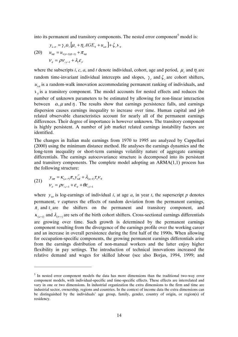
Ramos (2001) analyzed the dynamic structure of male fulltime employees’ earnings in Great Britain for the period 1991-99 by decomposing the earnings covariance structure

14

into its permanent and transitory components. The nested error component5 model is:

(20)

[ ]

ελρννπ

νζηµαγ

+=

+=+++=

−

−−

1,

)1)(1(

where the subscripts , , , and denote individual, cohort, age and period,

ηµ and are

random time-invariant individual intercepts and slopes,

ζγ and are cohort shifters,

is a random-walk innovation accommodating permanent ranking of individuals, and

ν is a transitory component. The model accounts for nested effects and reduces the

number of unknown parameters to be estimated by allowing for non-linear interaction between ηµα and, . The results show that earnings persistence falls, and earnings dispersion causes earnings inequality to increase over time. Human capital and job related observable characteristics account for nearly all of the permanent earnings differences. Their degree of importance is however unknown. The transitory component is highly persistent. A number of job market related earnings instability factors are identified.

The changes in Italian male earnings from 1970 to 1995 are analyzed by Cappellari (2000) using the minimum distance method. He analyses the earnings dynamics and the long-term inequality or short-term earnings volatility nature of aggregate earnings differentials. The earnings autocovariance structure is decomposed into its persistent and transitory components. The complete model adopting an ARMA(1,1) process has the following structure:

(21) 1,1,

)()(

−−

−−

++=

+=

θεερνντλπκ

where is log-earnings of individual , at age , in year , the superscript denotes

permanent, captures the effects of random deviation from the permanent earnings,

τπ and are the shifters on the permanent and transitory component, and

)()( and −− λκ are sets of the birth cohort shifters. Cross-sectional earnings differentials

are growing over time. Such growth is determined by the permanent earnings component resulting from the divergence of the earnings profile over the working career and an increase in overall persistence during the first half of the 1990s. When allowing for occupation-specific components, the growing permanent earnings differentials arise from the earnings distribution of non-manual workers and the latter enjoy higher flexibility in pay settings. The introduction of technical innovations increased the relative demand and wages for skilled labour (see also Borjas, 1994, 1999; and

5 In nested error component models the data has more dimensions than the traditional two-way error component models, with individual-specific and time-specific effects. These effects are interrelated and vary in one or two dimensions. In industrial organization the extra dimensions to the firm and time are industrial sector, ownership, regions and countries. In the context of income data the extra dimensions can be distinguished by the individuals’ age group, family, gender, country of origin, or region(s) of residency.

15

Atkinson, 1999). Another life cycle model of earnings dynamics with an ARMA(1,1) suggested by Moffitt and Gottschalk (2002) is written as:

(22) )()( 1,1,1,1,1,1, −−−−−− ++++=+=

ξθξρωµανµα

where the parameters of the model shift over time. The objective is to investigate the deriving force behind trends in the US widening earnings distribution. They fit stochastic earnings processes to the empirical covariance structure and decompose it into its permanent and transitory parts. Results based on earnings of a sample of 2988 male heads aged 20-59 from PSID during 1968-96 show that the variance of permanent earnings increased in the 1970s and 1980s, while the variance of transitory earnings rose in the 1980s and 1990s. The two components equally contributed to the growth of earnings inequality. Similar results were found by Baker and Solon (1998) using data on Canadian men. To compare the covariance structure of earnings by 16 cohorts and split the sample by occupation at age 22 into four skill groups, Dickens (2000) estimated the following model:

(23) ))(1())(1( 1,1,1,1,

2211,

221 −−−−− ++++++++=

+=

ξθξρδδωµαανµα

where the permanent and transitory components vary non-linearly over time according to a quadratic equations in 2121 and,, δδαα . The model is very complicated, yet the number of unknown parameters reduced by using an interaction of vectors of parameters. Results using UK individual earnings data over the period 1975-95 suggest that an individual’s earnings contain a highly permanent element, modelled by a random walk specification in age. The rise in earnings inequality was mainly driven by the permanent earnings differential in the first half of the 1980s, while later appear to be the outcome of earnings volatility. The increase in the variance of earnings is greater in the non-manual groups and is driven by changes in the transitory variance.

In sum a further classification of inequality decomposition can be made by the transitory and permanent nature of inequality. Here the focus is on the dynamics or changes in individual earnings from one period to another. The earnings covariance structure is decomposed into persistent and transitory components. Their contributions to the growth of earnings inequality by sub-groups are quantified. This is important in the design of policy measures and expectations about their impact on earnings inequality. Estimated permanent earning dynamics allow analyses of individual specific earnings profiles, and a few examples are found in Baker (1997), Baker and Solon (1998) and Cappellari (2000). Cappellari finds that the earnings profiles diverge with characteristics like age implying a widening of permanent differentials over the working career, with skills implying differences in permanent earnings growth among skilled and manual workers due to an increase in permanent differentials over time. A distinction between permanent and transitory components of earnings differentials has important implications for the understanding of changing inequality, the segmented distribution of household’s income and welfare. Rising earnings inequality may exacerbate a household’s poverty, and calls for interventions and design of policies aimed at alleviating such welfare-worsening effects (Gottschalk, 1997 and Gottschalk and Smeeding, 1997).

The path from wage shocks to resulting changes in the observed consumption allocation

16

decisions show associations with factors deriving from the income processes. Attanasio . (2002) argue that the simultaneous analysis of earnings and consumption data can add to our insights of the evolution of inequality. It can be helpful in decomposing shocks to earnings and wages not only into transitory and permanent components, but also to distinguish shocks that households are able to smooth out from those they are not, differentiating the responses to shocks with primary and secondary earners’ components of household earnings. Such information is important in the design of policy measures, in identification and quantification of their effects, and the distribution and the cost of their inequality alleviation. The presence of permanent and chronic inequality reduces the impact of inequality reducing policy measures.

Statistical inferences for inequality measurement, if any, are based on the asymptotic distribution of the index, the delta-method. One difficulty that arises in this context is the dependency in the data as inequality indices are often estimated based on a cross-section of a panel survey. To test for changes in the index over time, it is necessary to take into account the intertemporal covariance structure of incomes requiring calculation of covariances.

An alternative to the delta-method is the bootstrapping method. Previous studies suggest that bootstraping is an attractive alternative to the existing approximate asymptotic inference methods. It provides an estimate of the sampling distribution of inequality by resampling from the original survey, thus simulating the original sampling procedure. The method has advantages in small samples and accounts for stochastic dependencies without explicitly dealing with its covariance structure. Mills and Zandvakili (1997) using the bootstrap method to calculate confidence intervals for some inequality indices as well as for the components of a decomposition of the Theil coefficient by subgroups, and compare them with those obtained based on the delta-method. The results based on PSID and National Longitudinal Surveys (NLS) pre- and post-tax income data suggest that statistical inference is essential even when large samples are available, and that the bootstrap procedure appears to perform well in this setting.

The validity of the bootstrap method is also shown in the context of inequality, mobility and poverty measurement in Biewen (2002), where additional scenarios consider correlated data, panel attrition or non-response, decomposition by sub-groups or income sources and decomposition of inequality changes. The class of additively decomposable inequality () measure is:

(24)

10

1101

10

1

12,

,,,

1

,,,

)(

)(

)1()(

−−

−

=

−

=

=

=

⎥⎦⎤

⎢⎣⎡ −−=

=

+=

∑

∑

µµµµ

µ

αα αα

ααα

ααα

where and denote population share and relation income. The contribution of the

17

between-group component, the share of the within-group component of subgroup and the within-group inequality to the overall inequality are:

(25)

∑=

=

=

=

1

,,

,,,

,,

/

/

αα

ααα

ααα

.

Experiments based on German wage data show that a higher coverage accuracy can be obtained by using bootstrap procedures. The decomposition of the changes in inequality following Mookherjee and Shorrocks (1982) is:

(26)

∆+∆+∆+∆=∆−+

∆−+∆+∆≈∆=−

∑

∑ ∑∑

=

−

= ==

1

10,11,1

1 11

12

))(log()(

)log(

µµ

where bars indicate average values over two periods, ∆ is the difference operator,

∆∆∆∆ and,, stands for the contribution of changing levels of within-age group

inequality, changes in population shares of the age groups on the within group and between group components, and changes in mean incomes to the changes in overall inequality. Monte Carlo results suggest that confidence intervals based on the simplest possible bootstrap procedure achieve the same coverage accuracy as intervals obtained based on the conventional normal approximation and should be preferred in practice.

Maasoumi and Heshmati (2000) conduct bootstrap tests for the existence of first and second order stochastic dominance amongst Swedish income distributions over time and for several subgroups of immigrants and Swedes. Results are based on a sample of 43724 individuals observed for the period 1982-90. Two income definitions are used; pre-transfer and taxes gross income, and post-transfer and taxes disposable income. A comparison of the distribution of these two variables affords a partial view of Sweden’s welfare system. The focus is on the development of incomes of Swede’s and immigrant groups of single individuals identified by: country of origin, period of residence, age, education, gender, marital status and household size. The results suggest that although the sample of singles studied is a relatively homogenous segment of the population of individuals, first order dominance is rare, but second order dominance holds in several cases especially amongst disposable income distribution. Income and welfare policies favour the elderly, females, and larger families, while taxes and public transfers are shown to be effective measures in reducing the variance of disposable income. The higher the educational credentials, the higher are the burdens of this welfare equalization policy. The development of income for immigrants has been different than those of Swedes and strongly affected by their length of residence and country of origin. Maasoumi and Heshmati (2003) using a panel of household data obtained from PSID, and a bootstrapping method, find a number of strong dominance rankings, both between groups and over time, and in both gross and disposable incomes.

Van de gaer, Funnell and McCarthy (1999) name two ways of statistical inference with measures of inequality. One can use the bootstrap method to calculate bootstrapped

18

standard errors of inequality or of functions of inequality measures as illustrated above. Alternatively, one can try to establish the large sample distribution of the inequality measure. These distribution-free statistical inferences are then extended to cases where incomes are correlated. The Atkinson/Kolm and the Generalized Entropy measure of inequality in the population are written as:

(27) [ ] [ ][ ]

1

/1)(1

µµ θθ

θ −=

and

(28) [ ] [ ][ ] ⎟⎟⎠

⎞⎜⎜⎝

⎛−= 1

)(

1θ

θθ µ

µ

where )/()1( 2 θθ −= . Under the null hypothesis of equality of [ ] [ ]'and θθ ,

[ ] [ ]' θθ − is asymptotically normally distributed with mean 0 and asymptotic

variance given by:

(29) [ ] [ ] [ ]''1

' ,,,1

θθθ Ω

where

(30) [ ] [ ][ ]

[ ][ ]

[ ][ ]

[ ][ ] ⎥

⎥

⎦

⎤

⎢⎢

⎣

⎡−−=

−−

'1

11

'

2'1

1'

1

11

21

1

')()()()(

,

µµ

µµ

µµ

µµ θθθθθθθθ

θ .

Similarly under the null hypothesis of equality of [ ] [ ]'and θθ , [ ] [ ]' θθ − is

asymptotically normally distributed with mean 0 and asymptotic variance:

(31) [ ] [ ] [ ]''1

' ,,,1

θθθ Ω

where

(32) [ ] [ ][ ] [ ]( )

[ ][ ] [ ]( ) ⎥

⎥⎦

⎤

⎢⎢⎣

⎡−−−−= ++ θθ

θθθ

θθ

µµθµ

µµθµ

'1

1'1

'

1

11

',

where the [ ]',' ααΩ is the variance covariance matrix of two correlated incomes.

Accounting for correlated nature of samples is important in the comparison of inequality before and after taxes and transfers or looking at the evolution of the distribution of income over time using panel data. The framework is illustrated with data from the Irish household budget survey of 1994. The results suggest that the positive correlation between incomes before and after tax reduce the standard errors of the difference in inequality before and after taxation substantially.

Foster and Sen (1997) in their review of economic inequality after a quarter century suggest a new approach to inequality rankings based on normalized stochastic dominance. They find the new inequality criterion useful in ranking inequality of distributions with different means. Formby, Smith and Zheng (1999) show that

19

coefficient of variation (CV) is closely related to this new criterion. Specially, a monotonic transformation of coefficient of variation, 1/2(CV)2 is equal to the area between the second-degree normalized stochastic curve and the line of perfectly equal distribution.

! "

It is not common for empirical researchers to report Gini standard errors, though ideally they should be reported to enable researchers to make inferences about the index. Giles (2002) extends the OLS regression framework as an alternative to the jackknife, statistical resampling technique to get a large-sample approximation for the standard error of the Gini to seemingly unrelated regressions. The variance of Gini obtained from a three-step procedure is:

(33) 2/)ˆ(4)( θ=

where Gini can be written as:

(34) )/1(1)/ˆ2( −−= θ

and

(35) ⎥⎦⎤

⎢⎣⎡

⎟⎠⎞⎜

⎝⎛⎟

⎠⎞⎜

⎝⎛= ∑∑

==

11θ

is the weighted least squares estimator of +=θ , and

is a heteroscedastic

disturbance term. Penn World Table Data for 133 countries in the years 1950, 1975, 1980 and 1985 is used, and Giles provides a basis for various ways to test the robustness of the Gini coefficient to changes in the sample data. Karagiannis and Kovacevic (2000) suggest a method to calculate the jackknife variance estimator for the Gini coefficient by two passes through the data as:

(36) 12)(

1−+−−=

where is the sample size,

is the value of the Gini coefficient when the th

observation is taken out of the sample and is the Gini coefficient based on all observations. The jackknife standard error is then obtained by taking the square root of the variance. The advantage with this procedure is that it is simple to use but not in the case of Gini if there are many observations and each time an observation is dropped a new pseudo estimate of Gini must be calculated. Ogwang (2000) suggests an alternative regression interpretation of the Gini index which is then exploited to derive a simple algorithm in a seven-step procedure to compute its jackknife standard errors index using OLS regression. The method provides that incomes are sorted in ascending order and assuming heteroscedastic disturbances (weighted least squares).

The statistical approach to income inequality measurement is also discussed by Giorgi (1999) who focuses on the sampling properties of some inequality indices using distribution-free and parametric approaches. He considers two independent samples of

size 21 and , then [ ]))/ˆ()/ˆ/(()( 22112

σσ +− is asymptotically distributed

20

)1,0( , where denote income inequality. The distribution-free approach involves (jackknife and bootstrap) methods of testing a hypothesis or setting up a confidence interval which does not require assumptions on the form of the parent distribution. The parametric approach hypothesis that the form of the underlying distribution is known means the inequality measure is expressed as a function of the considered distribution.6 The iterated bootstrap method is applied in analysing the changes in income inequality over time based on sample data by Xu (1997). The results, based on a proposed method with bias correction on US income in 1969, 1979 and 1988, verify the statistical significance of the changes of income inequality during the 1970s and 1980s.

Schechtman and Yitzhakai (1999) show that the Gini correlation measures the dependence between two random variables, based on the covariance between one variable and the cumulative distribution of the other. Its properties are a mixture of Pearson’s and Spearman’s correlation measures, and they propose its application to decompose the Gini coefficient of household income into its components such as household heads, spouse and capital incomes. Another possible area of application is to analyze the variability of assets and their impacts on the stability of a finance portfolio.

The delta and bootstrapping methods are two alternatives in making inference for inequality measurement. The latter has advantages in that it avoids complicated covariance calculations, and is used to calculate confidence intervals for different subgroups, inequality within and between subgroups, inequality decomposed by income sources and for the components of a decomposed inequality index. For instance one looks at the evolution of the distribution of income over time using panel data and compares inequality over time before and after taxes and transfers for different subgroups. Other approaches used include the jackknife and regression methods to report Gini standard errors. A new approach to inequality rankings is based on normalized stochastic dominance useful in cases where distribution of income has different means.

This review focused on recent developments of inequality decomposition and decomposition of changes in poverty. The origin of the modern inequality decomposition literature is to be found in Shorrocks’ work. Inequality is decomposed by subgroups, income sources, causal factors and by other unit characteristics. Regression-based methods of decomposition of inequality by income sources have been proposed where standard income-generating equations written in terms of covariances are estimated. Compared with the unconditional approach, the regression-based methods, depending on the way modelled, provide possibilities to quantify the conditional roles of various characteristics in a multivariate context and allowing for heterogeneity in responses. Furthermore confidence intervals for disaggregated contributions to the inequality index can be constructed.

Different methods of decomposing changes in poverty into growth, redistribution,

6 The distributional assumptions involve: rectangular, exponential, Pareto, log-normal, Burr, Dagum and two-parameter gamma distributions.

21

poverty standard and residual components were described, where the aim is to study the effects of growth on poverty accounting for changes in the distribution of income and poverty standard. The first two components differ by the base year and the Lorenz curve reference level chosen as the benchmark. Depending on data availability different measures of income and poverty can be used, and such an exercise is important in the evaluation of the inequality impact of growth and its impacts on poverty among regions, subgroups and sectors.

It is important to distinguish between the transitory and permanent components of earnings. In the long-term some effects of transitory shocks average out, while other persists. Economic policy aiming to change earnings inequality should distinguish shocks that households are able to smooth out and target those that they can not smooth out by accounting for subgroup heterogeneity and earnings instability. Several recently introduced dynamic earnings models with various degrees of complexity and a summary of their findings based on household surveys are given. These parametric approaches are conditional of various covariates. The main benefits of parametric approaches are that changes are conditional on various attributes not all captured by the growth and redistribution components. Furthermore, confidence intervals for the effects are estimated. The main disadvantage is the assumption of functional forms of the relationships and its specification.

Statistical inferences for inequality measurement including delta and bootstrapping methods to provide estimates of the sampling distribution of inequality are discussed. The bootstrap method is used to calculate confidence intervals for different subgroups, within and between subgroups inequality, inequality decomposed by income sources, to compare inequality over time before and after taxes and transfers and for different subgroups. Jackknife and regression methods are employed to report Gini standard errors. The measurement, decomposition and modelling issues discussed here are crucial to the design of policy measures and expectations about their impacts on earnings inequality and poverty reductions.

22

Acemoglu D. (2002), Cross-country inequality trends, NBER Working Paper No. 8832. Acemoglu D. and J. Ventura (2002), The world income distribution, Quarterly Journal

of Economics CXVII(2), 659-694. Anand S. (1997), The measurement of income inequality, in: S. Subramanian (ed)

Measurement of inequality and poverty, Oxford University Press, pp. 81-105. Assadzadeh and Paul (2003), Poverty, growth and redistribution: A case-study of Iran,

in van der Hoeven R. and Shorrocks A., eds., Perspectives on growth and poverty, United Nations University Press, Tokyo.

Atkinson A.B. (1997), Bringing income distribution in from the cold, The Economic Journal 107, 297-321.

Atkinson A.B. (1999), Is rising inequality inevitable? A critique of the transatlantic consensus, The United Nations University, WIDER Annual Lectures 3, Helsinki: UNU/WIDER.

Atkinson A.B. and F. Bourguignon (1987), Income distribution and differences in needs, In: Feiwel G.R. (ed.), Arrow and Foundations of the Theory of Economic Policy, Macmillan, London.

Attanasio O., G. Berloffa, R. Blundell and I. Preston (2002), From earnings inequality to consumption inequality, The Economic Journal 112, March C52-C59.

Baker M. (1997), Growth-rate heterogeneity and the covariance structure of life-cycle earnings, Journal of Labor Economics 15(2), 338-375.

Baker M. and G. Solone (1998), Earnings dynamics and inequality among Canadian men, 1976-1992: evidence from longitudinal income tax records, Institute for Policy Analysis, University of Toronto, mimeo.

Barro R.J. (1991), Economic growth in a cross section of countries, Quarterly Journal of Economics 106, 406-443.

Barro R.J. and X. Sala-i-Martin (1995), Economic Growth, McGraw-Hill Inc. Biewen M. (2002a), Bootstrap inference for inequality, mobility and poverty

measurement, Journal of Econometrics 108(2), 317-342. Borjas G.J. (1994), The economics of immigration, Journal of Economic Literature 31

December, 1667-1717. Borjas G.J. (1999), Economic research on the determinants of immigration: lessons for

the European Union, World Bank Technical Paper No. 438. Bourguignon F. and F.G. Fournier and M. Gurgend (2001), Fast development with a

stable income distribution in Taiwan, 1979-94, Review of Income and Wealth 47(2), 139-163.

Bourguignon F. and C. Morrisson (2002), Inequality among world citizens: 1820-1992, American Economic Reviews 92(4), 727-747.

Burtless G. (1999), Effects of growing wage disparities and changing family composition on the U.S. income distribution, European Economic Review 43, 853-865.

Cameron L.A. (2000b), Poverty and inequality in Java: examining the impact of the changing age, educational and industrial structure, Journal of Development Economics 62, 149-180.

Caminada K. and K. Goudswaard (2001), International trends in income inequality and social policy, International Tax and Public Finance 8(4), 395-415.

Cappellari L. (2000), The dynamics and inequality of Italian male earnings: permanent changes or transitory fluctuations?, Institute for Social and Economic Research.

23

Cappellari L. and S.P. Jenkins (2002), Who stays poor? Who becomes poor? Evidence from the British household panel survey, The Economic Journal 112, March C60-C67.

Chiu W.H. (1998), Income inequality, human capital accumulation and economic performance, The Economic Journal 108, 44-59.

Chotikapanich D. and W. Griffiths (2001), On calculation of the extended Gini coefficient, Review of Income and Wealth 47(4), 541-547.

Chotikapanich D. and W. Griffiths (2002), Estimating Lorenz curves using a Dirichlet distribution, Journal of Business and Economic Statistics 20, 290-295.

Cornia G.A. (1999), Liberalization, globalization and income distribution, WIDER Working Paper 1999/157, Helsinki: UNU/WIDER.

Cornia G.A. and S. Kiiski (2001), Trends in income distribution in the post WWII period: evidence and interpretation, WIDER Discussion Paper 2001/89, Helsinki: UNU/WIDER.

Cowell F.A. (2000), Measurement of inequality, in Atkinson A.B. and Bourguignon F. (Eds), Handbook of Income Distribution, Volume 1, North Holland, chapter 2, 87-166.

Cowell F.A. and S.P. Jenkins (1995), How much inequality can we explain? A methodology and an application to the USA, Economic Journal 105(429), 421-430.

Cowell F.A. and M-P. Victoria-Feser (1996a), Robustness properties of inequality measures, Econometrica 64(1), 77-101.

Cowell F.A. and M-P. Victoria-Feser (1996b), Poverty measurement with contaminated data: a robust approach, European Economic Review 40, 1761-1771.

Datt G. and M. Ravallion (1992), Growth and redistribution components of changes in poverty measures: A decomposition with applications to Brazil and India in the 1980, Journal of Development Economics 38, 275-295.

Dhongde S. (2002), Measuring the impact of growth and income distribution on poverty: an analysis of the States of India, Unpublished manuscript.

Dickens (2000), The evolution of individual male earnings in Great Britain: 1975-95, The Economic Journal 110, January 27-49.

DiNardo J., N.M. Fortin and T. Lemieux (1996), Labor market institutions and the distribution of wages, 1973-1992: a semiparametric approach, Econometrica 64,5, 1001-1044.

Duro J.A. and J. Esteban (1998), Factor decomposition of cross-country income inequality, 1960-1990, Economics Letters 60, 269-275.

Fields G.S. (2000), Measuring Inequality Change in an Economy with Income Growth, The International Library of Critical Writings in Economics: Income Distribution, (Edward Elgar).

Formby J.P., W.J. Smith and B. Zheng (1999), The coefficient of variation, stochastic dominance and inequality: a new interpretation, Economics Letters 62, 319-323.

Foster J.E. and A. Sen (1997), On economic inequality after a quarter century, In: On economic inequality, expanded ed., Clarendon Press, oxford.

Georlich-Gisbert F.J. (2001), On factor decomposition of cross-country income inequality: some extensions and qualifications, Economics Letters 70, 303-309.

Geweke J. and M. Keane (2000), An empirical analysis of earnings dynamics among men in the PSID: 1968-1989, Journal of Econometrics 96, 293-356.

Giles D.E.A. (2002), Calculating a standard error for the Gini coefficient: some further

24

results, University of Victoria, Depart of Economics, Working paper EWP0202. Giorgi. G.M. (1999), Income inequality measurement: the statistical approach, in Silber

J. and A. Sen (eds), Handbook of income inequality measurement, chapter 8, pp. 245-267, Kluwer Academic Publishers.

Gottschalk P. (1997), Inequality, income growth, and mobility: the basic facts, Journal of Economic Perspectives 11(2), 21-40.

Gottschalk P. and T.M Smeeding (1997), Cross-national comparisons of earnings and income inequality, Journal of Economic Literature 35, 633-687.

Gottschalk P. and T.M. Smeeding (2000), Empirical evidence on income inequality in industrialized countries, in Atkinson A.B. and Bourguignon F. (Eds), Handbook of Income Distribution, Volume 1, North Holland, chapter 5, pp.261-308.

Hasegawa H. and H. Kozumi (2003), Estimation of Lorenz curves: a Bayesian nonparametric approach, Journal of Econometrics 115, 277-291.

Heshmati A. (2004), Inequalities and their measurement, Unpublished Manuscript. Huck S., H-T. Norman and J. Oechssler (2001), Market volatility and inequality in

earnings: experimental evidence, Economics Letters 70, 363-368. Islam N. (1995), Growth empirics: a panel data approach, The Quarterly Journal of

Economics 110, 1127-1170. Jenkins S.P. (1995), Accounting for inequality trends: decomposition analysis for the

UK, Economica 62, 29-64. Jenkins S.P. and P. Van Kerm (2003), Trends in income inequality, prop-poor income

growth and income mobility, IZA Discussion Paper 2003:904. Jian L.R. and Tendulkar (1990), Role of growth and distribution in the observed change

of headcount ratio-measure of poverty: a decomposition exercise for India, Technical report no. 9004 (Indian Statistical Institute, Delhi).

Kakwani N. and K. Subbarao (1990), Rural Poverty and its alleviation in India, Economic and Political Weekly, March 31, 1990.

Karagiannis E. and M. Kovacevic (2000), A method to calculate the Jackknife variance estimator for the Gini coefficient, Oxford Bulletin of Economics and Statistics 62, 119-122.

Lee K., M.H. Pesaran and R. Smith (1997), Growth and convergence in a multi-country empirical stochastic Solow model, Journal of Applied Econometrics 12, 357-392.

Lerman R.I. and S. Yitzhaki (1989), Improving the accuracy of estimates of Gini coefficients, Journal of Econometrics 42(1), 43-47.

Maasoumi E. and A. Heshmati (2000), Stochastic dominance amongst Swedish income distributions, Econometric Reviews 19(3), 287-320.

Maasoumi E. and A. Heshmati (2003), Evaluating dominance ranking of PSID incomes by various household characteristics, Unpublished manuscript.

Mankiew N.G., D. Romer and D.H. Weil (1992), A contribution to the empirics of economics growth, The Quarterly Journal of Economics 107, 407-438.

Milanovic B. (2002a), True world income distribution, 1988 and 1993: First calculation based on household surveys alone, Economic Journal 112(476), 51-92.

Mills A.M. and S. Zandvakili (1997), Statistical inference via bootstrapping for measures of inequality, Journal of Applied Econometrics 12, 133-150.

Moffitt R.A. and P. Gottschalk (2002), Trends in the transitory variance of earnings in the United States, The Economic Journal 112, March C68-C73.

Mookherjee D. and A. Shorrocks (1982), A decomposition analysis of the trends in UK income inequality, The Economic Journal 92(368), 886-902.

25

Morduch J. and T. Sicular (2002), Rethinking inequality decomposition, with evidence from rural China, Economic Journal 112(476), 93-106.

Ogwang T. (2000), A convenient method of computing the Gini index and its standard error, Oxford Bulletin of Economics and Statistics 62, 1, 123-129.

Ogwang T. and U.L.G. Rao (2000), Hybrid models of the Lorenz curve, Economics Letters 69, 39-44.

Ok E.A. and P. Lambert (1999), On evaluating social welfare by sequential generalized Lorenz dominance, Economics Letters 63, 45-53.

O’Rourke K.H. (2001), Globalization and inequality: historical trends, NBER Working Paper 8339, Cambridge MA: NBER.

Park D. (2001), Recent trends in the global distribution of income, Journal of Policy Modeling 23, 497-501.

Pyatt G. (1976), On the interpretation and disaggrgation of Gini coefficient, Economic Journal 86(342), 243-255.

Quah D. (1996c), Empirics for economic growth and convergence, European Economic Review 40, 1353-1375.

Quah D. (2002), One third of the world’s growth and inequality, Economics Department, CEPR Discussion Paper 2002:3316.

Ramos X. (2001), The dynamics of individual male earnings in Great Britain: 1991-1999; Universitat Autonoma de Barcelona, Spain.

Ravallion M. (2003b), Inequality convergence, Economics Letters 80, 351-356. Ryu H.K. and D.J. Slottje (1999), Parametric approximation of the Lorenz Curve, in S.

Silber and A. Sen (eds), Handbook of Income Distribution, Chapter 10, 291-314, Kluwer Academic Press.

Sala-i-Martin X. (2002a), The disturbing “Rise” of global income inequality, NBER Working Paper Series 8904.

Sala-i-Martin X. (2002b), The world distribution of income (estimated from individual country distribution), NBER Working Paper 8933.

Schechtman E. and S. Yitzhaki (1999), On the proper bounds of the Gini correlation, Economics Letters 63, 133-138.

Schultz T.P. (1998), Inequality in distribution of personal income in the world: how it is changing and why, Journal of Population Economics 11(3), 307-344.

Shorrocks A.F. (1980), The class of additively decomposable inequality, Econometrica 48(3), 613-625.

Shorrocks A.F. (1982), Inequality decomposition by factor components, Econometrica 50(1), 193-211.

Shorrocks A.F. (1983), The impact of income components on the distribution of family incomes, Quarterly Journal of Economics 98,2, 311-326.

Shorrocks (1984), Inequality decomposition by population subgroups, Econometrica 52(6), 1369-1385.

Shorrocks A. and S. Kolenikov (2001), Poverty trends in Russia during the transition, Unpublished manuscript.

Shorrocks A. and G. Wan (2003), Spatial decomposition of inequality, Unpublished manuscript.

Solimano A. (2001), The evolution of world income inequality: assessing the impact of globalization, Unpublished manuscript, ECLAC, CEPAL – Serie Macroeconomica del desarrollo No. 11, Santiago, Chile.

Subramanian S. (1997a), (ed.), Measurement of inequality and poverty, Readers in

26

Economics, Oxford University Press. Sylwester K. (2000), Income inequality, education expenditures, and growth, Journal of

Development Economics 63, 379-398. Van de gaer D. Funnel N. and T. McCarthy (1999), Statistical inference for two

measures of inequality when incomes are correlated, Economics Letters 64, 295-300.

Xu K. (1997), Inference for generalized Gini indices using the iterated bootstrap method, Department of Economics, Dalhousie University, Canada.

Yitzhaki S. (1983), On an extension of the Gini inequality index, International Economic Review 24(3), 617-628.

Yitzhaki S. (2002), Do we need a separate poverty measurement?, European Journal of Political Economy 18, 61-85.

Zandvakili S. (1999), Income inequality among female heads of households: racial inequality reconsidered, Economica 66, 119-133.

Zandvakili S. (2000), Dynamics of earnings inequality among female-headed households in the United States, Journal of Socio-Economics 29, 73-89.

Zandvakili S. (2002), Trends in earnings inequality among young adults, Review of Social Economy 60(1), 93-107.

Zandvakili S. and J.A. Mills (2001), The distributional implications of tax and transfer programs in US, The Quarterly Review of Economics and Finance 41, 167-181.