impact of indian ocean sea surface temperature on...

Impact of Indian Ocean Sea Surface Temperature on Developing El Niño*

H. ANNAMALAI, S. P. XIE, AND J. P. MCCREARY

International Pacific Research Center, University of Hawaii, Honolulu, Hawaii

R. MURTUGUDDE

ESSIC, University of Maryland, College Park, College Park, Maryland

(Manuscript received 12 March 2004, in final form 22 July 2004)

ABSTRACT

Prior to the 1976–77 climate shift (1950–76), sea surface temperature (SST) anomalies in the tropicalIndian Ocean consisted of a basinwide warming during boreal fall of the developing phase of most El Niños,whereas after the shift (1977–99) they had an east–west asymmetry—a consequence of El Niño beingassociated with the Indian Ocean Dipole/Zonal mode. In this study, the possible impact of these contrastingSST patterns on the ongoing El Niño is investigated, using atmospheric reanalysis products and solutions toboth an atmospheric general circulation model (AGCM) and a simple atmospheric model (LBM), with thelatter used to identify basic processes. Specifically, analyses of reanalysis products during the El Niño onsetindicate that after the climate shift a low-level anticyclone over the South China Sea was shifted into the Bayof Bengal and that equatorial westerly anomalies in the Pacific Ocean were considerably stronger. Thepresent study focuses on determining influence of Indian Ocean SST on these changes.

A suite of AGCM experiments, each consisting of a 10-member ensemble, is carried out to assess therelative importance of remote (Pacific) versus local (Indian Ocean) SST anomalies in determining precipi-tation anomalies over the equatorial Indian Ocean. Solutions indicate that both local and remote SSTanomalies are necessary for realistic simulations, with convection in the tropical west Pacific and thesubsequent development of the South China Sea anticyclone being particularly sensitive to Indian OceanSST anomalies. Prior to the climate shift, the basinwide Indian Ocean SST anomalies generate an atmo-spheric Kelvin wave associated with easterly flow over the equatorial west-central Pacific, thereby weak-ening the westerly anomalies associated with the developing El Niño. In contrast, after the shift, theeast–west contrast in Indian Ocean SST anomalies does not generate a significant Kelvin wave response,and there is little effect on the El Niño–induced westerlies. The Linear Baroclinic Model (LBM) solutionsconfirm the AGCM’s results.

1. Introduction

It is now well recognized that the El Niño–SouthernOscillation (ENSO) phenomenon is the dominantmode of tropical climate variability. Moreover, thechanges in tropical precipitation and associated latent-heat release during ENSO affect the atmospheric cir-culation globally, primarily through wave dynamics(Hoskins and Karoly 1981; Shukla and Wallace 1983;Sardeshmukh and Hoskins 1985; Trenberth et al. 1998;Su et al. 2001). In comparison to the large fluctuations

in sea surface temperature (SST) in the equatorial Pa-cific during ENSO, interannual SST anomalies in theIndian Ocean are modest. As a consequence, under-standing their effect on the atmosphere has receivedless attention.

Recently, interest in the influence of Indian OceanSSTs has expanded considerably, in part due to thedebate about the Indian Ocean “Dipole/Zonal” mode(IODZM), a mode of climate variability associatedwith cooling in the eastern equatorial Indian Oceanduring fall and warming in the western basin severalmonths later (Reverdin et al. 1986; Murtugudde et al.1998; Saji et al. 1999; Webster et al. 1999; Murtuguddeand Busalacchi 1999; Behera et al. 1999; Yu and Rie-necker 1999, 2000). The high simultaneous correlationbetween IODZM and Niño-3.4 SST anomalies occursduring fall, suggesting that IODZM events are forcedby ENSO (e.g., Allan et al. 2001; Baquero-Bernal et al.2002; Xie et al. 2002; Hastenrath 2002; Krishnamurthyand Kirtman 2003; Annamalai et al. 2003). Others ar-gue that the extreme events of 1961, 1994, and 1997 are

* International Pacific Research Center Contribution Number293 and School of Ocean and Earth Science and Technology Con-tribution Number 6364.

Corresponding author address: Dr. H. Annamalai, IPRC/SOEST, University of Hawaii, 1680 East West Rd., Honolulu, HI96822.E-mail: [email protected]

302 J O U R N A L O F C L I M A T E VOLUME 18

JCLI3268

a coupled ocean–atmosphere mode internal to the In-dian Ocean itself (e.g., Yamagata et al. 2003). As dis-cussed below, a likely reason for the differing views isthat the relationship between El Niño and IODZMevents has changed in time.

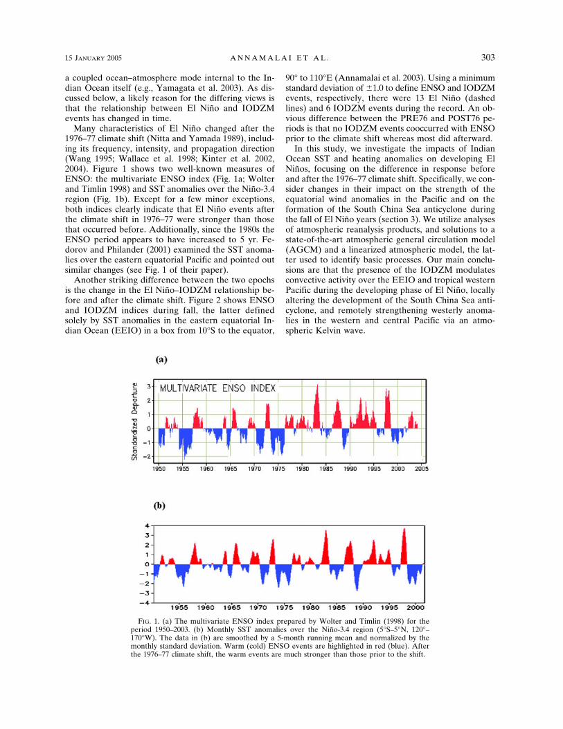
Many characteristics of El Niño changed after the1976–77 climate shift (Nitta and Yamada 1989), includ-ing its frequency, intensity, and propagation direction(Wang 1995; Wallace et al. 1998; Kinter et al. 2002,2004). Figure 1 shows two well-known measures ofENSO: the multivariate ENSO index (Fig. 1a; Wolterand Timlin 1998) and SST anomalies over the Niño-3.4region (Fig. 1b). Except for a few minor exceptions,both indices clearly indicate that El Niño events afterthe climate shift in 1976–77 were stronger than thosethat occurred before. Additionally, since the 1980s theENSO period appears to have increased to 5 yr. Fe-dorov and Philander (2001) examined the SST anoma-lies over the eastern equatorial Pacific and pointed outsimilar changes (see Fig. 1 of their paper).

Another striking difference between the two epochsis the change in the El Niño–IODZM relationship be-fore and after the climate shift. Figure 2 shows ENSOand IODZM indices during fall, the latter definedsolely by SST anomalies in the eastern equatorial In-dian Ocean (EEIO) in a box from 10°S to the equator,

90° to 110°E (Annamalai et al. 2003). Using a minimumstandard deviation of �1.0 to define ENSO and IODZMevents, respectively, there were 13 El Niño (dashedlines) and 6 IODZM events during the record. An ob-vious difference between the PRE76 and POST76 pe-riods is that no IODZM events cooccurred with ENSOprior to the climate shift whereas most did afterward.

In this study, we investigate the impacts of IndianOcean SST and heating anomalies on developing ElNiños, focusing on the difference in response beforeand after the 1976–77 climate shift. Specifically, we con-sider changes in their impact on the strength of theequatorial wind anomalies in the Pacific and on theformation of the South China Sea anticyclone duringthe fall of El Niño years (section 3). We utilize analysesof atmospheric reanalysis products, and solutions to astate-of-the-art atmospheric general circulation model(AGCM) and a linearized atmospheric model, the lat-ter used to identify basic processes. Our main conclu-sions are that the presence of the IODZM modulatesconvective activity over the EEIO and tropical westernPacific during the developing phase of El Niño, locallyaltering the development of the South China Sea anti-cyclone, and remotely strengthening westerly anoma-lies in the western and central Pacific via an atmo-spheric Kelvin wave.

FIG. 1. (a) The multivariate ENSO index prepared by Wolter and Timlin (1998) for theperiod 1950–2003. (b) Monthly SST anomalies over the Niño-3.4 region (5°S–5°N, 120°–170°W). The data in (b) are smoothed by a 5-month running mean and normalized by themonthly standard deviation. Warm (cold) ENSO events are highlighted in red (blue). Afterthe 1976–77 climate shift, the warm events are much stronger than those prior to the shift.

15 JANUARY 2005 A N N A M A L A I E T A L . 303

Fig 1 live 4/C

It should be noted that our study uses stand-aloneatmospheric models to investigate changes in ENSOvariability, which surely involve coupled air–sea inter-actions. Indeed, recent coupled modeling studies (e.g.,Wu and Kirtman 2004a) suggest that experiments withprescribed SST anomalies over the Indian Ocean maydistort the air–sea feedbacks between latent heat fluxand SST, which lead to spurious variance in rainfall andsurface wind anomalies. Our AGCM results must beviewed with this caveat in mind. On the other hand, ourfocus is to understand the large-scale response to In-dian Ocean SST anomalies. The fact that the simulatedwinds over the equatorial Pacific by both the AGCMand the simple linear atmospheric model bear close re-semblance to observations suggests our approach is rea-sonable.

The paper is organized as follows. Section 2 presentsthe data used and provides a brief description of theAGCM and LBM. Section 3 presents diagnostic analy-ses based on observations. Section 4 examines the sen-sitivity of the AGCM to Indo–Pacific SST anomalies.Section 5 examines the dynamical response of the LBMto diabatic heating and SST anomalies. Section 6 sum-marizes our conclusions.

2. Data and models

a. Data

The atmospheric data used in our study are takenfrom National Centers for Environmental Prediction–

National Center for Atmospheric Research (NCEP–NCAR) reanalysis products for the period 1950–2001(Kalnay et al. 1996). The atmospheric variables areavailable at standard pressure levels with a horizontalresolution of 2.5°. The SST for the analysis period istaken from Reynolds and Smith (1994).

In the data analyses, monthly mean climatologies arefirst calculated for the study period and anomalies aredepartures from them. Unless specified otherwise, de-cadal variability (periods � 8 yr) is separated from in-terannual variability (16 months to 8 yr) through har-monic analysis. Composites are formed for the strongEl Niño years during both epochs (Fig. 2a), except thatthe 1986–87 event is excluded because of the complex-ity of its evolution with respect to the annual cycle(Wang et al. 2000) and the lack of IODZM develop-ment (Fig. 2b). Due to uncertainities in SST observa-tions prior to the satellite era, we compared themonthly Reynolds and Smith (1994) product with theComprehensive Ocean–Atmosphere Data Set(COADS). As in Fig. 2, we formed interannual SSTanomalies over EEIO and Niño-3.4 regions (notshown) from COADS. We note high correlations(�0.7) between the corresponding indices constructedfrom these two datasets.

The composites (both constructed from observationsand from ensembles of AGCM solutions) are subjectedto the standard t test for statistical significance, and onlywhen at the 95% significant level are retained in plots;the sole exception is for Fig. 4b, in which values signifi-cant at the 85% level are retained due to the limitedmembers (four) in the composites. The level of signifi-cance does not alter the main conclusions of the presentstudy that are supported by dynamical arguments (sec-tions 4–5).

Concerning the 1986–87 event, an examination ofmonthly SST anomalies over the Nino-3.4 region (notshown) reveals that (i) the onset of El Niño occurredduring boreal summer 1986 and attained its first peakintensity in December of that year, (ii) the amplitude ofthe warm SST anomalies gradually declined from 1.2°Cin December 1986 to 0.7°C in June 1987, and (iii) theamplitude suddenly increased and reached its secondpeak (�1.7°C) in September 1987; and thereafter ElNiño conditions ceased. Thus, the evolution of the1986–87 El Niño differs markedly from other major ElNiños. The Simple Ocean Data Assimilation (SODA)product, as well as solutions from ocean models, indi-cate that the mean thermocline was deeper than normalin the EEIO during the El Niño events of 1976 and1986–87, conditions unfavorable for the developmentof the IODZM (Annamalai et al. 2004, manuscript sub-mitted to J. Climate). Since our purpose is to under-stand the influence of the cooccurrence of IODZMevents with developing El Niño in the post-1976 epoch,we excluded the 1986–87 event in our analysis. With theexclusion of the 1986–87 event, all El Niño events in thepost-1976 composite are accompanied by concurrent

FIG. 2. Bar charts of the boreal fall (SON) SST anomalies for (a)the Niño-3.4 region (5°S–5°N, 120°–170°W) and (b) eastern equa-torial Indian Ocean region (10°S–0°, 90°–110°E). The dotted hori-zontal lines represent �1.0 standard deviation in (b) and �1.0standard deviation in (a). The SST anomalies are normalized withtheir respective standard deviations.


IOZM events while none is in the pre-1976 composite.This grouping allows us to study the effect of differingIndian Ocean SST patterns by AGCM experimentationto be described in section 4a.

Various diagnostic studies have assessed the qualityof reanalyses in the Tropics, showing that the divergentpart of the wind is strongly influenced by model heat-ing, especially in data-sparse regions (e.g., Annamalaiet al. 1999). For example, Kinter et al. (2004) attributedinterdecadal changes in the divergent wind field in theNCEP–NCAR reanalysis to changes in the observingsystem and assimilation procedures [see also Wu andXie (2003)]. Since decadal and interdecadal variabilityis removed in our analysis prior to making composites,effects due to changes in the observing system are mini-mized.

b. AGCM

The AGCM we use is the ECHAM5, the latest Ham-burg version of the ECMWF model. It is a global spec-tral model, which we ran at T42 resolution and with 19sigma levels in the vertical. The nonlinear terms and theparameterized physical processes are calculated on a128 � 64 Gaussian grid with a horizontal resolution ofabout 2.8° � 2.8°. As in the earlier version of the model(ECHAM4, Roeckner et al. 1996), the convectionscheme is based on the mass-flux concept of Tiedtke(1989); the surface fluxes of momentum, heat, watervapor, and cloud water are based on the Monin–Obukhov similarity theory, and the radiation scheme isdue to Morcrette et al. (1998). Major changes to thephysical package include implicit coupling of the atmo-sphere to the land surface (Schulz et al. 2001), advectivetransport (Lin and Rood 1996), a prognostic–statisticalscheme for cloud cover (Tompkins 2002), and a rapidradiative-transfer model for longwave radiation(Mlawer et al. 1997). Model details can be found inRoeckner et al. (2003).

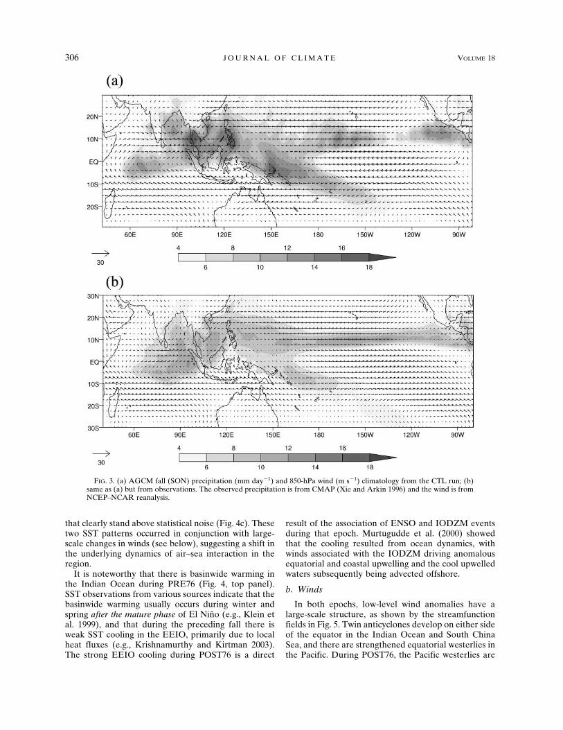
The climatology of ECHAM5 is realistic in many as-pects. Figure 3 shows precipitation and 850-hPa windduring September–October–November (SON) for themodel (Fig. 3a) and the observations (Fig. 3b). Mod-el � observation differences include (i) overestimationof precipitation intensity over the tropical western Pa-cific and along the South Pacific convergence zone(SPCZ), (ii) a westward shift in the location of the pre-cipitation maximum and poleward orientation of west-erlies over the equatorial Indian Ocean, and (iii) cross-equatorial flow in the western Indian Ocean and pen-etration of westerlies into the tropical west Pacific.Despite these differences, the spatial structure andmagnitude of precipitation and low-level circulationanomalies over the tropical Indo–Pacific regions aresimulated reasonably well.

c. LBM

Linear atmospheric models have been widely used asa diagnostic tool for studying the response to idealized

forcing (e.g., Matsuno 1966; Webster 1972; Gill 1980;Rodwell and Hoskins 1996). The linear model we use(labeled LBM) is fully described in Watanabe andKimoto (2000) and Watanabe and Jin (2003). It is aglobal, time-dependent, primitive-equation model, lin-earized about the observed climatology derived fromNCEP–NCAR reanalysis for 1958–97. Its horizontalresolution is T21 with 20 vertical levels in sigma coor-dinates. The model employs diffusion, Rayleigh fric-tion, and Newtonian damping with a time scale of (1day)�1 for � � 0.9 and � � 0.03, while (30 day)�1 isused elsewhere.

The LBM is forced either by prescribed patterns ofdiabatic heating anomalies or SST anomalies, referredto as dry and moist versions respectively (Watanabeand Jin 2003). In the dry version, the prescribed forcingis the anomalous diabatic heating proportional to theobserved precipitation anomalies. The horizontal shapeof the heating is elliptical and the heating is imposed onboreal fall (September–November) mean climatologyderived from NCEP–NCAR reanalysis. The verticalheating profile is defined by an empirical function pro-posed by Reed and Recker (1971), with a maximumheating at 400 hPa. Since in the deep Tropics heatingand circulation are strongly coupled, we also seek thesteady-state response in which the LBM calculates itsown heating. In this run, called moist case, the horizon-tal shape of the prescribed SST anomalies is assumed tobe elliptical as in the dry case. The surface heat fluxgenerated by these forcings is parameterized as in Bettsand Miller (1986). A linearized moisture equation forthe perturbation specific humidity is incorporated intothe model. Heat and moisture sources associated withcumulus convection are also parameterized. In themoist case, mean fields of SST and ground wetness arealso included in the basic state. In summary, resultsfrom the moist case can be viewed as an alternative tothe AGCM solutions but within the linear framework.

3. Air–sea interaction during El Niño onset

In this section, we report the differences in SST andcirculation patterns between the PRE76 and POST76periods. Due to nonavailability of observed precipita-tion products over the oceans during PRE76 we havenot compared the changes in the precipitation here.However, model solutions reported in section 4 illus-trate the differences in the simulated precipitation tothe apparent changes in SST that were used to force theAGCM.

a. SST

Figure 4 shows SST-anomaly composites from Reyn-olds and Smith (1994) during the fall of El Niño yearsbefore (PRE76, 1950–76) and after (POST76, 1977–99)the climate shift. During POST76 there were coherentcold SST anomalies in the EEIO and western Pacific


that clearly stand above statistical noise (Fig. 4c). Thesetwo SST patterns occurred in conjunction with large-scale changes in winds (see below), suggesting a shift inthe underlying dynamics of air–sea interaction in theregion.

It is noteworthy that there is basinwide warming inthe Indian Ocean during PRE76 (Fig. 4, top panel).SST observations from various sources indicate that thebasinwide warming usually occurs during winter andspring after the mature phase of El Niño (e.g., Klein etal. 1999), and that during the preceding fall there isweak SST cooling in the EEIO, primarily due to localheat fluxes (e.g., Krishnamurthy and Kirtman 2003).The strong EEIO cooling during POST76 is a direct

result of the association of ENSO and IODZM eventsduring that epoch. Murtugudde et al. (2000) showedthat the cooling resulted from ocean dynamics, withwinds associated with the IODZM driving anomalousequatorial and coastal upwelling and the cool upwelledwaters subsequently being advected offshore.

b. Winds

In both epochs, low-level wind anomalies have alarge-scale structure, as shown by the streamfunctionfields in Fig. 5. Twin anticyclones develop on either sideof the equator in the Indian Ocean and South ChinaSea, and there are strengthened equatorial westerlies inthe Pacific. During POST76, the Pacific westerlies are

FIG. 3. (a) AGCM fall (SON) precipitation (mm day�1) and 850-hPa wind (m s�1) climatology from the CTL run; (b)same as (a) but from observations. The observed precipitation is from CMAP (Xie and Arkin 1996) and the wind is fromNCEP–NCAR reanalysis.


stronger, the northern anticyclone is weaker and shiftedfrom the South China Sea into the Bay of Bengal, andthe southern anticyclone is strengthened over the southIndian Ocean. Composite maps of 850-hPa windanomalies (not shown) are consistent with the stream-function fields.

It is noteworthy that during POST76 the South ChinaSea anticyclone is not well developed (Fig. 5b), despitethe higher intensity of SST anomalies over the Niño-3.4region, and the stronger atmospheric response over theequatorial Pacific including the substantial local nega-tive precipitation anomalies (Fig. 6b). To substantiate

FIG. 4. Boreal fall composites of SST anomalies (°C) during El Niño years: (a) PRE76 and (b)POST76, and (c) their difference [(a) � (b)]. PRE76 (POST76) corresponds to the period 1950–75(1977–99). The El Niño events selected during PRE76 are 1953, 1957, 1963, 1965, 1969, 1972, and 1976,and those during POST76 are 1982, 1991, 1994, and 1997. The shading interval is 0.2°C for the top twopanels and 0.15°C for the bottom panel.


Fig 4 live 4/C

this result, Fig. 5c shows the monthly composite timeseries of 850-hPa streamfunction anomalies averagedover the tropical west Pacific. During PRE76 (solidline) a weak anticyclonic signature persists from Aprilonward and rapidly intensifies in October. In contrast,during POST76 (dashed line) a weak cyclonic signalpersists from the beginning of the year, peaking in Sep-tember. Thereafter, its sign reverses but the resultinganticyclone is much weaker than its counterpart duringPRE76.

Several prior studies have noted the climatic impor-tance of the South China Sea anticyclone. Harrison andLarking (1996) first reported its presence in the westernPhilippine Sea during the winter of El Niño years.Wang et al. (2000) showed that it initially develops inthe South China Sea, and that it subsequently modu-lates the East Asian monsoon, leading to strongersoutherlies and enhanced precipitation over SoutheastAsia. Wang et al. (2000) used both simple and compre-hensive AGCMs to demonstrate that the anticyclone

FIG. 5. Boreal fall composites of 850-hPa streamfunction anomalies for (a) PRE76 and (b)POST76, and (c) monthly composite evolution of 850-hPa streamfunction anomalies averagedover (0°–20°N, 100°–130°E), for PRE76 (solid) and POST76 (dashed). The units are m2 s�1.


forms as a Rossby wave response to anomalous diabaticcooling associated with the weakened convection overthe Maritime Continent, and Watanabe and Jin (2003)used the LBM (section 2) to arrive at the same conclu-sion. While Wang et al. (2000) suggested that the weak-ened convection is primarily associated with the east-ward shift of climatological convection over the Pacificduring El Niño, Watanabe and Jin (2003) emphasizedthat the basinwide warm SST anomalies in the IndianOcean also contribute, acting to strengthen local con-vection, weaken the ascending branch of the IndianOcean Walker circulation, and hence, decrease convec-tion over the Maritime Continent. In a simple tropicalmodel, Su et al. (2001) noted similar effects during thewinter of the 1997–98 El Niño. In contrast, Lau andNath (2000) concluded that the Philippine Sea anticy-clone in their AGCM solutions was sensitive to Pacific

SST anomalies alone. We show next that the spatialdistribution of SST anomalies in the tropical IndianOcean during fall exert considerable influence on theformation of the South China Sea anticyclone noted inFig. 5.

4. Solutions to the AGCM

In this section, we report a suite of AGCM experi-ments designed to assess the influence of Indian andPacific Ocean SST anomalies on a developing El Niñoduring the PRE76 and POST76 epochs. The experi-mental design is first discussed (section 4a), then themodel’s ability in simulating the basic response to In-do–Pacific SST anomalies is discussed (section 4b), andthen the effect of Indian Ocean (section 4c) SSTanomalies on the Pacific is presented.

FIG. 6. (a) Anomalous precipitation (mm day�1, shaded) and 850-hPa wind anomalies from the TIP_POST solutions;(b) same as (a) but from observations.


Fig 6 live 4/C

a. Experimental design

Six AGCM experiments are carried out, divided intothree groups. In the tropical Indo–Pacific (TIP) runs,seasonally varying SST anomalies associated with ElNiño are imposed in the tropical Indo–Pacific regionfrom 30°S to 30°N during both PRE76 and POST76epochs (as shown for SON in Fig. 4), and seasonallyvarying climatological SSTs are imposed elsewhere. Werefer to the two sets as TIP_PRE and TIP_POST runs,respectively. The tropical Pacific Ocean (TPO_PREand TPO_POST) runs are similar to the two TIP runs,except that SST anomalies are inserted only in thetropical Pacific. Similarly, the tropical Indian Ocean(TIO_PRE and TIO_POST) runs are like the TIP runs,but SST anomalies are imposed only in the tropicalIndian Ocean. These sets of experiments are expectedto reveal the individual and combined effects of SSTanomalies on the local and remote climate variability.For instance, the difference between TIP and TPO so-lutions will suggest the effect of Indian Ocean SSTanomalies when the Pacific SST effect is interactivewhile that of the TIO and TPO solutions will indicatethe exclusive and noninteractive effect of the individualoceans. The primary motivation for conducting theseexperiments is as follows: the SST anomalies over thetropical Indian Ocean often cooccur with those in thetropical Pacific and therefore it is difficult, if not im-possible, to quantify their effects separately from ob-servations alone, and experiments with an AGCMforced with SST anomalies in each ocean basin offer ameans to study their separate effects.

For each of the six forcing scenarios, the model is runfor the 2 yr covering the life cycle of El Niño events,that is, from 1 January of year(0) to 31 December ofyear(1). To account for the atmospheric sensitivity toinitial conditions, a 10-member ensemble approach,with changes only in the initial conditions selected from10 snapshots of the climatological control run but pre-serving the same SST forcing, is conducted for eachforcing scenario. Initial conditions are taken from thecontrol (CTL) run in which the seasonally varying cli-matological SST was used as the boundary forcing.Table 1 provides some details of the experiments. Sincethe IODZM over the equatorial Indian Ocean peaks

during boreal fall season (e.g., Saji et al. 1999), themodel results are only presented for fall season of year(0), that is, during the developing phase of El Niño. Ina companion study, Annamalai and Liu (2004, manu-script submitted to Quart. J. Roy. Meteor. Soc., hereaf-ter ALQJR) examine the model response during borealsummer to understand the response of the summermonsoon due to the changes in ENSO properties dur-ing POST76.

b. Basic response to Indo–Pacific SST anomalies

For brevity, we have not shown all of the individualTIP and TPO solutions. To assess the AGCM’s fidelityin simulating the basic response, as an example, weshow the TIP_POST solutions (Fig. 6a) and comparethem with observations (Fig. 6b). Both in model solu-tions and observations, during POST76, a band of en-hanced precipitation eastward of 170°E occupies theequatorial Pacific while reduced precipitation coversthe tropical west Pacific, extending into the MaritimeContinent. The east–west dipole pattern in precipita-tion over the equatorial Pacific is a well-known featureduring El Niño years (e.g., Lau and Nath 2000). It israther interesting to note that negative precipitationanomalies over the EEIO (�60%–70% reduction of itsclimatological value) are flanked by positive anomaliesin the western Indian Ocean (Figs. 6a,b). This east–westcontrast in precipitation anomalies over the equatorialIndian Ocean is associated with corresponding changesin the SST distribution (Fig. 4b). While westerly windanomalies dominate the equatorial Pacific, easterlywind anomalies prevail over the equatorial IndianOcean. In summary, the salient features of the indi-vidual TIP and TPO solutions include (i) all four solu-tions have similar spatial distribution of precipitationand wind anomalies over the Pacific demonstrating thedominant influence of Pacific SST anomalies in deter-mining the atmospheric response there and (ii) the so-lutions obtained by the TIP_POST and TPO_POSTruns indicate that about 20%–25% of the EEIO pre-cipitation variability is forced by Pacific SST anomaliesalone. The close similarity between the model solutionsand observations (e.g., Fig. 6) paves the way for isolat-ing and understanding the possible effect of IndianOcean SST anomalies on the Pacific climate.

c. Influence of Indian Ocean SST anomalies

First, we show the TIP � TPO difference plot (Fig.7), which will shed light on the local and remote impactof Indian Ocean SST anomalies that can be directlycompared with TIO solutions (Fig. 8). The differencebetween the TIP_PRE and TPO_PRE runs (Fig. 7a)indicates substantial anomalies of precipitation not onlyin the Indian Ocean but in the tropical West Pacific aswell. During PRE76, basinwide positive precipitationanomalies over the Indian Ocean are accompanied by asignificant reduction in precipitation and anticyclonic

TABLE 1. A list of the AGCM experiments discussed in the text.

Expt Forcing

CTL Climatological but seasonally varying SSTTIP_PRE PRE76 El Niño SST anomalies over the tropical

Indo–Pacific (40ºE–80ºW) regionsTIP_POST Same as TIP_PRE but for POST76TPO_PRE PRE76 El Niño SST anomalies over the tropical

Pacific only (120ºE–80ºW)TPO_POST Same as TPO_PRE but for POST76TIO_PRE PRE76 El Niño SST anomalies only over the

tropical Indian Ocean (40º–120ºE)TIP_POST Same as TIO_PRE but for POST76


circulation anomalies over the tropical west Pacific(Fig. 7a). In contrast, during POST76 an east–west gra-dient in precipitation along the equatorial IndianOcean is accompanied by near-normal precipitationover the tropical west Pacific (Fig. 7b). Therefore, thischange in precipitation response in the tropical westPacific and the lack of the South China Sea anticycloneduring POST76 (Fig. 7b) attest to changes in the heat-ing distributions in the equatorial Indian Ocean.

To isolate the effect of Indian Ocean SST on thePacific, additional experiments forced with only the In-dian Ocean SST anomalies are carried out. An addi-tional advantage of the TIO runs is that they aid inassessing the nonlinearity by comparing with the TIP �TPO difference maps (e.g., Fig. 7). The large-scale re-sponse, however, appears to be linear in that anomaliesare similar in Figs. 7 and 8 except for the positive pre-cipitation anomalies over the equatorial central Pacific

and associated westerly wind anomalies during POST76(Fig. 7b). Thus, the inclusion of Indian Ocean SSTanomalies together with those over the tropical Pacificresults in an increase in precipitation over the equato-rial Pacific possibly due to nonlinear and interactiveeffects.

In TIO_PRE, as a direct response to basinwide warmSST anomalies, precipitation increases over the tropicalIndian Ocean (Fig. 8a) and easterly (westerly) windanomalies dominate the eastern (western) IndianOcean but slightly north (south) of the equator. Con-sistent with observations (section 3), in the AGCM so-lutions that include the effect of Indian Ocean SSTanomalies, the most conspicuous feature in the TIO_PRErun is the suppression of precipitation over the tropi-cal west Pacific and its enhancement in the IndianOcean. The precipitation response in the TIO_POSTrun differs considerably from that in TIO_PRE. In the

FIG. 7. AGCM-simulated precipitation difference (mm day�1) in color shading and 850-hPa wind (m s�1) differencebetween the TIP and TPO solutions during fall. This figure highlights the role of Indian Ocean SST anomalies in local andremote variations in precipitation and 850-hPa winds.


Fig 7 live 4/C

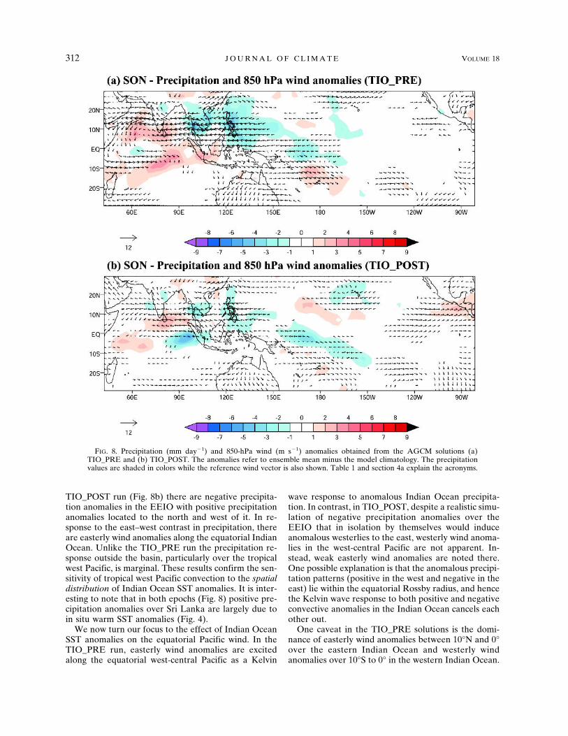
TIO_POST run (Fig. 8b) there are negative precipita-tion anomalies in the EEIO with positive precipitationanomalies located to the north and west of it. In re-sponse to the east–west contrast in precipitation, thereare easterly wind anomalies along the equatorial IndianOcean. Unlike the TIO_PRE run the precipitation re-sponse outside the basin, particularly over the tropicalwest Pacific, is marginal. These results confirm the sen-sitivity of tropical west Pacific convection to the spatialdistribution of Indian Ocean SST anomalies. It is inter-esting to note that in both epochs (Fig. 8) positive pre-cipitation anomalies over Sri Lanka are largely due toin situ warm SST anomalies (Fig. 4).

We now turn our focus to the effect of Indian OceanSST anomalies on the equatorial Pacific wind. In theTIO_PRE run, easterly wind anomalies are excitedalong the equatorial west-central Pacific as a Kelvin

wave response to anomalous Indian Ocean precipita-tion. In contrast, in TIO_POST, despite a realistic simu-lation of negative precipitation anomalies over theEEIO that in isolation by themselves would induceanomalous westerlies to the east, westerly wind anoma-lies in the west-central Pacific are not apparent. In-stead, weak easterly wind anomalies are noted there.One possible explanation is that the anomalous precipi-tation patterns (positive in the west and negative in theeast) lie within the equatorial Rossby radius, and hencethe Kelvin wave response to both positive and negativeconvective anomalies in the Indian Ocean cancels eachother out.

One caveat in the TIO_PRE solutions is the domi-nance of easterly wind anomalies between 10°N and 0°over the eastern Indian Ocean and westerly windanomalies over 10°S to 0° in the western Indian Ocean.

FIG. 8. Precipitation (mm day�1) and 850-hPa wind (m s�1) anomalies obtained from the AGCM solutions (a)TIO_PRE and (b) TIO_POST. The anomalies refer to ensemble mean minus the model climatology. The precipitationvalues are shaded in colors while the reference wind vector is also shown. Table 1 and section 4a explain the acronyms.


Fig 8 live 4/C

Examination of a composite of observed winds at 850hPa for PRE76 (Fig. 5a) reveals the dominance of east-erly wind anomalies over the equatorial Indian Ocean(10°S–10°N). This systematic error in the TIO_PRE so-lutions appears to be a Rossby wave response to thepositive precipitation anomalies over the equatorialwestern central Indian Ocean. Presumably, they are re-lated to systematic errors in the model mean precipita-tion climatology in the western Indian Ocean notedearlier (Fig. 3a).

5. Solutions to the LBM

An AGCM’s response to imposed SST anomaliesgenerally depends on the model’s basic state (e.g.,Shukla 1984; Lau and Nath 2000; Kang et al. 2002). Inthe AGCM used here, a deficiency of the basic state isthe westward shift in the precipitation climatology overthe equatorial Indian Ocean (Fig. 3a) and the associ-ated error in the simulated wind anomalies discussed insection 4c. For this reason, here we consider solutionsto the LBM, for which the background state is pre-scribed. The LBM solutions therefore provide an alter-nate, and clarifying, view of the basic dynamics.

a. Experimental design

As mentioned in section 2, solutions are obtained forboth dry and moist versions of the LBM, forced byidealized diabatic heating and SST anomalies, respec-tively, that mimic observed precipitation patterns in theequatorial Indian Ocean.

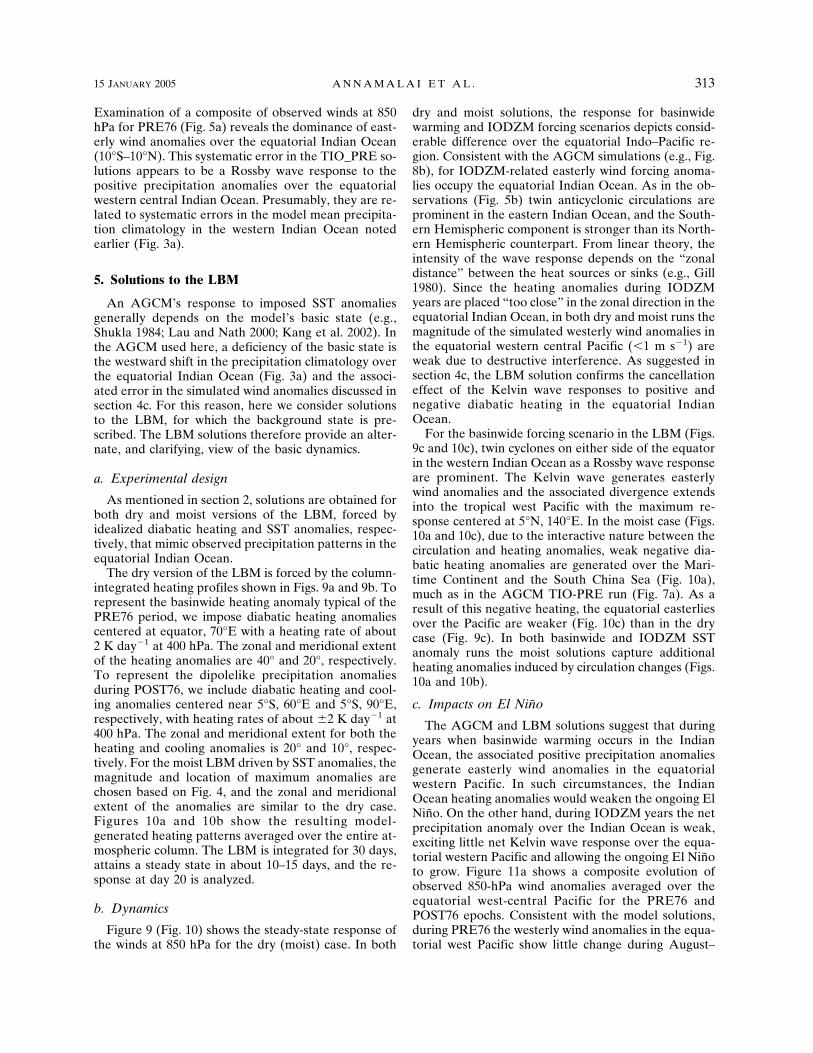
The dry version of the LBM is forced by the column-integrated heating profiles shown in Figs. 9a and 9b. Torepresent the basinwide heating anomaly typical of thePRE76 period, we impose diabatic heating anomaliescentered at equator, 70°E with a heating rate of about2 K day�1 at 400 hPa. The zonal and meridional extentof the heating anomalies are 40° and 20°, respectively.To represent the dipolelike precipitation anomaliesduring POST76, we include diabatic heating and cool-ing anomalies centered near 5°S, 60°E and 5°S, 90°E,respectively, with heating rates of about �2 K day�1 at400 hPa. The zonal and meridional extent for both theheating and cooling anomalies is 20° and 10°, respec-tively. For the moist LBM driven by SST anomalies, themagnitude and location of maximum anomalies arechosen based on Fig. 4, and the zonal and meridionalextent of the anomalies are similar to the dry case.Figures 10a and 10b show the resulting model-generated heating patterns averaged over the entire at-mospheric column. The LBM is integrated for 30 days,attains a steady state in about 10–15 days, and the re-sponse at day 20 is analyzed.

b. Dynamics

Figure 9 (Fig. 10) shows the steady-state response ofthe winds at 850 hPa for the dry (moist) case. In both

dry and moist solutions, the response for basinwidewarming and IODZM forcing scenarios depicts consid-erable difference over the equatorial Indo–Pacific re-gion. Consistent with the AGCM simulations (e.g., Fig.8b), for IODZM-related easterly wind forcing anoma-lies occupy the equatorial Indian Ocean. As in the ob-servations (Fig. 5b) twin anticyclonic circulations areprominent in the eastern Indian Ocean, and the South-ern Hemispheric component is stronger than its North-ern Hemispheric counterpart. From linear theory, theintensity of the wave response depends on the “zonaldistance” between the heat sources or sinks (e.g., Gill1980). Since the heating anomalies during IODZMyears are placed “too close” in the zonal direction in theequatorial Indian Ocean, in both dry and moist runs themagnitude of the simulated westerly wind anomalies inthe equatorial western central Pacific (�1 m s�1) areweak due to destructive interference. As suggested insection 4c, the LBM solution confirms the cancellationeffect of the Kelvin wave responses to positive andnegative diabatic heating in the equatorial IndianOcean.

For the basinwide forcing scenario in the LBM (Figs.9c and 10c), twin cyclones on either side of the equatorin the western Indian Ocean as a Rossby wave responseare prominent. The Kelvin wave generates easterlywind anomalies and the associated divergence extendsinto the tropical west Pacific with the maximum re-sponse centered at 5°N, 140°E. In the moist case (Figs.10a and 10c), due to the interactive nature between thecirculation and heating anomalies, weak negative dia-batic heating anomalies are generated over the Mari-time Continent and the South China Sea (Fig. 10a),much as in the AGCM TIO-PRE run (Fig. 7a). As aresult of this negative heating, the equatorial easterliesover the Pacific are weaker (Fig. 10c) than in the drycase (Fig. 9c). In both basinwide and IODZM SSTanomaly runs the moist solutions capture additionalheating anomalies induced by circulation changes (Figs.10a and 10b).

c. Impacts on El Niño

The AGCM and LBM solutions suggest that duringyears when basinwide warming occurs in the IndianOcean, the associated positive precipitation anomaliesgenerate easterly wind anomalies in the equatorialwestern Pacific. In such circumstances, the IndianOcean heating anomalies would weaken the ongoing ElNiño. On the other hand, during IODZM years the netprecipitation anomaly over the Indian Ocean is weak,exciting little net Kelvin wave response over the equa-torial western Pacific and allowing the ongoing El Niñoto grow. Figure 11a shows a composite evolution ofobserved 850-hPa wind anomalies averaged over theequatorial west-central Pacific for the PRE76 andPOST76 epochs. Consistent with the model solutions,during PRE76 the westerly wind anomalies in the equa-torial west Pacific show little change during August–


FIG

.9.(

a)V

erti

calc

olum

n–in

tegr

ated

diab

atic

heat

ing

anom

alie

s(K

day�

1)

impo

sed

for

the

basi

nwid

ew

arm

ing

scen

ario

;(b)

sam

eas

(a)

butf

orIO

DZ

Mhe

atin

g;(c

)pe

rtur

bati

onw

ind

resp

onse

at85

0hP

afo

rhe

atin

gpa

tter

nsh

own

in(a

);an

d(d

)sa

me

as(c

)bu

tfo

rth

ehe

atin

gpa

tter

nsh

own

in(b

).T

heL

BM

isru

nin

“dry

”m

ode.

Con

tour

inte

rval

in(a

)an

d(b

)is

0.2

Kda

y�1

and

the

refe

renc

ew

ind

vect

ors

for

(c)

and

(d)

are

also

show

n.


FIG

.10.

As

inF

ig.1

0bu

tfor

the

moi

stL

BM

run.

SST

anom

alie

sas

show

nin

Fig

.2ar

epr

escr

ibed

and

the

mod

el-g

ener

ated

heat

ing

anom

alie

s(K

day�

1)

inte

grat

edov

erth

eve

rtic

alco

lum

nar

esh

own

in(a

)an

d(b

),an

dth

eco

rres

pond

ing

850-

hPa

win

d(m

s�1)

and

stre

amfu

ncti

on(1

06m

2s�

1)

anom

alie

sar

esh

own

insh

adin

gin

(c)

and

(d),

resp

ecti

vely

.T

heco

ntou

rin

terv

als

in(a

)an

d(b

)ar

e0.

2K

day.

The

shad

ing

inte

rval

sin

(c)

and

(d)

are

0.5e

�06

;neg

ativ

eva

lues

are

show

nas

cont

ours

whi

lepo

siti

veva

lues

are

shad

ed.


November. In sharp contrast in POST76, the anoma-lous westerlies amplify rapidly in July–October, a pe-riod during which the Sumatra cooling grows andreduces the Indian Ocean effect on the west Pacific.

Our results from observations and AGCM and LBMsolutions paint a coherent picture that Indian Oceanheating anomalies do influence the amplitude of thezonal wind anomalies in the equatorial west-central

FIG. 11. (a) Composite evolution of zonal wind anomalies (m s�1) averaged over the equa-torial west-central Pacific during PRE76 (black line) and POST76 (red line) El Niños, root-mean-square variance of SST (°C) during Dec–Feb during (b) PRE76 and (c) POST76.


Pacific, which in turn impact the thermocline in theeastern equatorial Pacific and affect the growth/development of El Niño in the Pacific (e.g., McCreary1976). The 1982–83 and 1997–98 El Niños, the strongestevents on record, are likely to be aided in their growthby the cooling over the EEIO. The observed SST vari-ance at the peak phase of ENSO (December–February)clearly indicates that the POST76 ENSO events aremuch stronger than those in PRE76 (Figs. 11b,c).

As mentioned in the introduction previous studieshave identified the changes in the strength of El Niñoduring POST76 (e.g., Wallace et al. 1998). Many factorsinfluence the statistical properties of El Niño, namely(i) nonlinearity (Timmermann et al. 2003; An and Jin2004), (ii) decadal variability in the mean state (Fe-dorov and Philander 2001; Wang and An 2001), (iii)stochastic forcing (Timmermann and Jin 2002), (iv)monsoon variability (e.g., Wainer and Webster 1996;Chung and Nigam 1999; Kirtman and Shukla 2000; Wuand Kirtman 2003), and (v) convective anomalies overthe equatorial west Pacific (Nicholls 1984; Weisbergand Wang 1997). The strongest El Niño of the previouscentury occurred during 1997–98 when Pacific decadalvariability was in its transition phase. During IODZMyears in POST76, the July–August rainfall over themonsoon region increased despite the suppressing ef-fect of El Niño (e.g., Annamalai et al. 2003; ALQJR).Therefore, among other factors, the dramatic changesin the spatial distribution of SST anomalies over theIndian Ocean (Fig. 4) may have also played a role in theamplification of the ongoing El Niño events. Landseaand Knaff (2000) presented the limitations of state-of-art coupled general circulation models (CGCMs) inpredicting the intensity of the 1997–98 El Niño. If ourhypothesis is correct, then El Niño events with cooc-curring IODZM events are stronger than those with-out, a preposition being tested currently by the authorsin CGCMs.

d. Impacts on the South China Sea anticyclone

Both AGCM and LBM solutions indicate that thebasinwide warming in the Indian Ocean induces diver-gence over the western Pacific that reduces the precipi-tation there and aids in rapid development of the anti-cyclone over the South China Sea (Fig. 10c). In con-trast, during IODZM years the net Kelvin waveresponse is too weak to exert any influence on westPacific convection (Fig. 10d). This simple mechanism,possibly, explains why the anticyclone developed dur-ing PRE76 but not in POST76.

6. Summary and discussion

In the present study, we investigate teleconnectionsfrom the equatorial Indian Ocean to the Pacific. Morespecifically, we explore the hypothesis that atmosphericKelvin waves, generated by convective anomalies in the

equatorial Indian Ocean during fall of El Niño years,establish equatorial wind anomalies that subsequentlyinfluence the ongoing El Niño.

To identify the influence of equatorial Indian OceanSST anomalies, we made composites of the SST andstreamfunction field at 850 hPa over the tropical Indo–Pacific regions separately for PRE76 (1950–75) andPOST76 (1977–99) El Niño events (section 3). In bothepochs, the anomalous heating and associated circula-tion response in the equatorial Pacific are overall simi-lar. Over the Indian Ocean, however, a basinwidewarming (east–west gradient) prevails in SST anoma-lies during PRE76 (POST76). An important differencebetween the epochs is the formation (absence) of theSouth China Sea anticyclone during PRE76 (POST76).Despite the higher intensity of SST anomalies over theNiño-3.4 region during POST76, the lack of a SouthChina Sea anticyclone is attributed to the differences inthe Indian Ocean SST anomalies.

To assess the relative roles of local versus remoteforcing on the convective anomalies over the IndianOcean, a suite of atmospheric model experiments iscarried out (section 4a). Using the AGCM, 10-memberensemble simulations, separately for PRE76 andPOST76 El Niño events, are conducted. The AGCMresults demonstrate that tropical west Pacific convec-tion and the subsequent development of the SouthChina Sea anticyclone are sensitive to Indian OceanSST anomalies (section 4c). In the PRE76 case, thebasinwide SST anomalies over the Indian Ocean forceeasterly wind anomalies over the near-equatorial west-ern central Pacific, whereas in POST76 the east–westcontrast in the SST anomalies weaken the easterly windanomalies over the equatorial Pacific (section 4c).

During IODZM years, the positive and negative pre-cipitation anomalies over the tropical Indian Ocean ex-ist well within the dissipation radius of Kelvin waves,resulting in the cancellation of the Kelvin wave re-sponse to this zonal dipole of precipitation anomalies.In sharp contrast, the Kelvin wave response to basin-wide heating anomalies in the Indian Ocean promoteseasterly wind anomalies over the tropical west Pacific.In either case, circulation anomalies induced by IndianOcean heating anomalies can modulate the ongoing ElNiño. In the former (latter) case, it would strength(weaken) the ongoing El Niño.

Idealized experiments with a linear model indicatethat the Kelvin wave response cancels out when bothpositive and negative heating anomalies coexist alongthe equatorial Indian Ocean. Based on the dynamicalinterpretations offered here, it is our opinion that theIODZM in POST76, to a certain degree, would havecontributed to the intensity of the El Niños in POST76.Our results are, however, constrained by the limitednumber of samples during POST76, and to overcomethis we are currently analyzing a long run of a coupledmodel.

Observational studies (Barnett 1983; Behera and


Yamagata 2003) and coupled modeling studies (e.g.,Anderson and McCreary 1985; Yu et al. 2002; Wu andKirtman 2004b) indicate that circulation anomaliesforced by Indian Ocean SST anomalies can influenceSST variance in the equatorial Pacific. Our results fur-ther strengthen these recent studies. Therefore, identi-fication of the Indian Ocean effect on El Niño calls foraccurate measurement of SST and surface wind overthe tropical Indian Ocean and further studies on itsdynamics.

Acknowledgments. This research is supported by theNOAA–OGP CLIVAR Pacific Program and by the Ja-pan Agency for Marine–Earth Science and Technology(JAMSTEC) through its sponsorship of the Interna-tional Pacific Research Center (IPRC). Additional sup-port is provided by the K. C. Wong Education Foun-dation (SPX) and NOAA Grant NA03OAR4310124(RM). The Max Planck Institute makes the ECHAMmodel available to the IPRC under a cooperativeagreement. Dr. Watanabe is acknowledged for provid-ing the linear model and offering valuable suggestionson its use. Dr. Niklas Schneider shared his experiencewith the COADS dataset. Valuable comments from theanonymous reviewers are greatly appreciated.

REFERENCES

Allan, R. J., and Coauthors, 2001: Is there an Indian Ocean dipoleindependent of the El Niño-Southern Oscillations? CLIVARExchanges, Vol. 6, No. 3, International CLIVAR Project Of-fice, Southampton, United Kingdom, 18–22.

An, S. I., and F. F. Jin, 2004: Nonlinearity and asymmetry ofENSO. J. Climate, 17, 2399–2412.

Anderson, D. L. T., and J. P. McCreary, 1985: On the role of theIndian Ocean in a coupled ocean–atmosphere model of ElNiño and the Southern Oscillation. J. Atmos. Sci., 42, 2439–2444.

Annamalai, H., H., J. M. Slingo, K. R. Sperber, and K. Hodges,1999: The mean evolution and variability of the Asian sum-mer monsoon: Comparison of ECMWF and NCEP–NCARreanalyses. Mon. Wea. Rev., 127, 1157–1186.

——, R. Murtugudde, J. Potemra, S. P. Xie, P. Liu, and B. Wang,2003: Coupled dynamics in the Indian Ocean: Spring initia-tion of the zonal mode. Deep-Sea Res., 50B, 2305–2330.

Baquero-Bernal, A., M. Latif, and S. Legutke, 2002: On dipolelikevariability of sea surface temperature in the tropical IndianOcean. J. Climate, 15, 1358–1368.

Barnett, T. P., 1983: Interaction of the monsoon and Pacific tradewind system at interannual time scales. Part I: The equatorialzone. Mon. Wea. Rev., 111, 756–773.

Behera, S. K., and T. Yamagata, 2003: Influence of the IndianOcean dipole on the Southern Oscillation. J. Meteor. Soc.Japan, 81, 169–177.

——, R. Krishnan, and T. Yamagata, 1999: Unusual ocean–atmosphere conditions in the tropical Indian Ocean during1994. Geophys. Res. Lett., 26, 3001–3004.

Betts, A., and M. J. Miller, 1986: A new convective adjustmentscheme. Part II: Single column tests using GATE wave,BOMEX, ATEX, and artic air-mass data sets. Quart. J. Roy.Meteor. Soc., 112, 693–709.

Chung, C., and S. Nigam, 1999: Asian summer monsoon–ENSO

feedback on the Cane–Zebiak model ENSO. J. Climate, 12,2787–2807.

Fedorov, A. V., and G. H. Philander, 2001: A stability analysis oftropical ocean–atmosphere interactions: Bridging measure-ments and theory for El Niño. J. Climate, 14, 3086–3101.

Gill, A. E., 1980: Some simple solutions for heat induced tropicalcirculation. Quart. J. Roy. Meteor. Soc., 106, 447–462.

Harrison, D. E., and N. K. Larking, 1996: The COADS sea levelpressure signal: A near-global El Niño composite and timeseries view, 1946–93. J. Climate, 9, 3025–3055.

Hastenrath, S., 2002: Dipoles, temperature gradients, and tropicalclimate anomalies. Bull. Amer. Meteor. Soc., 83, 735–740.

Hoskins, B. J., and D. J. Karoly, 1981: The steady linear responseof a spherical atmosphere to thermal and orographic forcing.J. Atmos. Sci., 38, 1179–1196.

Kalnay, E., and Coauthors, 1996: NCEP/NCAR 40-Year Reanaly-sis Project. Bull. Amer. Meteor. Soc., 77, 437–471.

Kang, I.-S., and Coauthors, 2002: Intercomparison of GCM simu-lated anomalies associated with the 1997–98 El Niño. J. Cli-mate, 15, 2791–2805.

Kinter, J. L., K. Miyakoda, and S. Yang, 2002: Recent changes inthe connection from the Asian monsoon to ENSO. J. Cli-mate, 15, 1203–1215.

——, M. J. Fennessy, V. Krishnamurthy, and L. Marx, 2004: Anevaluation of the apparent interdecadal shift in the tropicaldivergent circulation in the NCEP–NCAR reanalysis. J. Cli-mate, 17, 349–361.

Kirtman, B. P., and J. Shukla, 2000: Influence of the Indian sum-mer monsoon on ENSO. Quart. J. Roy. Meteor. Soc., 126,1–27.

Klein, S. A., B. J. Soden, and N. C. Lau, 1999: Remote sea surfacetemperature variations during ENSO: Evidence for a tropicalatmospheric bridge. J. Climate, 12, 917–932.

Krishnamurthy, V., and B. P. Kirtman, 2003: Variability of theIndian Ocean: Relation to monsoon and ENSO. Quart. J.Roy. Meteor. Soc., 129, 1623–1646.

Landsea, C. W., and J. A. Knaff, 2000: How much skill was therein forecasting the very strong 1997–98 El Niño. Bull. Amer.Meteor. Soc., 81, 2107–2119.

Lau, N. C., and M. J. Nath, 2000: Impact of ENSO on the vari-ability of the Asian–Australian monsoon as simulated inGCM experiments. J. Climate, 13, 4287–4309.

Lin, S. J., and R. B. Rood, 1996: Multidimensional flux fromLagrangian transport. Mon. Wea. Rev., 124, 2046–2086.

Matsuno, T., 1966: Quasi-geostrophic motions in the equatorialarea. J. Meteor. Soc. Japan, 44, 25–43.

McCreary, J. P., 1976: Eastern tropical ocean response to chang-ing wind systems: With application to El Niño. J. Phys.Oceanogr., 6, 632–645.

Mlawer, E. J., S. J. Taubman, P. D. Brown, M. J. Iacono, and S. A.Clough, 1997: Radiative transfer for inhomogeneous atmo-sphere: RRTM, a validated correlated-k model for the long-wave. J. Geophys. Res., 102, 16 663–16 682.

Morcrette, J. J., S. A. Clough, E. J. Mlawer, and M. J. Iacono,1998: Impact of a validated radiative transfer scheme,RRTM, on the ECMWF model climate and 10-day forecasts.ECMWF Tech. Memo. 252, Reading, United Kingdom, 47 pp.

Murtugudde, R., and A. J. Busalacchi, 1999: Interannual variabil-ity of the dynamics and thermodynamics of the tropical In-dian Ocean. J. Climate, 12, 2300–2326.

——, B. N. Goswami, and A. J. Busalacchi, 1998: Air–sea inter-action in the southern tropical Indian Ocean and its relationsto interannual variability of the monsoon over India. Proc.Int. Conf. on Monsoon and Hydrologic Cycle, Kyongju, Ko-rea, Korean Meteorological Society.

—— J. P. McCreary, and A. J. Busalacchi, 2000: Oceanic pro-cesses associated with anomalous events in the Indian Oceanwith relevance to 1997–98. J. Geophys. Res., 105, 3295–3306.

Nicholls, N., 1984: The Southern Oscillation and Indonesian seasurface temperature. Mon. Wea. Rev., 112, 424–432.


Nitta, T., and S. Yamada, 1989: Recent warming of tropical seasurface temperature and its relationship to the NorthernHemisphere circulation. J. Meteor. Soc. Japan, 67, 375–383.

Reed, R. J., and E. E. Recker, 1971: Structure and properties ofsynoptic-scale wave disturbances in the equatorial westernPacific. J. Atmos. Sci., 28, 1117–1133.

Reverdin, G., D. Cadet, and D. Gutzler, 1986: Interannual dis-placements of convection and surface circulation over theequatorial Indian Ocean. Quart. J. Roy. Meteor. Soc., 112,43–46.

Reynolds, R. W., and T. M. Smith, 1994: Improved global seasurface temperature analyses using optimal interpolation. J.Climate, 7, 929–948.

Rodwell, M. J., and B. J. Hoskins, 1996: Monsoons and the dy-namics of desert. Quart. J. Roy. Meteor. Soc., 122, 1385–1404.

Roeckner, E., and Coauthors, 1996: Atmospheric general circula-tion model ECHAM4: Model description and simulation ofpresent-day climate. Max-Planck-Institut für MeteorlogieRep. 218, Hamburg, Germany, 82 pp.

——, and Coauthors, 2003: Atmospheric general circulationmodel ECHAM5: Part I. Max-Planck-Institut für Meteorlo-gie Rep. 349, Hamburg, Germany, 140 pp.

Saji, N. H., B. N. Goswami, P. N. Vinayachandran, and T. Yama-gata, 1999: A dipole mode in the tropical Indian Ocean. Na-ture, 401, 360–363.

Sardeshmukh, P. D., and B. J. Hoskins, 1985: Vorticity balances inthe tropics during the 1982–83 El Niño–Southern Oscillationevent. Quart. J. Roy. Meteor. Soc., 111, 261–278.

Schulz, J. P., L. Dumenil, and J. Polcher, 2001: On the land surfaceatmosphere coupling and its impact in a single column atmo-spheric model. J. Appl. Meteor., 40, 642–663.

Shukla, J., 1984: Predictability of time averages: Part II. The in-fluence of the boundary forcing. Problems and Prospects inLong and Medium Range Weather Forecasting, D. M. Bur-ridge and E. Kallen, Eds., Springer-Verlag, 155–206.

——, and J. M. Wallace, 1983: Numerical simulation of the atmo-spheric response to equatorial Pacific sea surface tempera-ture anomalies. J. Atmos. Sci., 40, 1613–1630.

Su, H., J. D. Neelin, and C. Chou, 2001: Tropical teleconnectionand local response to SST anomalies during the 1997–98 ElNiño. J. Geophys. Res., 106, 20 025–20 043.

Tiedtke, M., 1989: A comprehensive mass flux scheme for cumu-lus parameterization in a large-scale model. Mon. Wea. Rev.,117, 1779–1800.

Timmermann, A., and F. F. Jin, 2002: A nonlinear mechanism fordecadal El Niño amplitude changes. Geophys. Res. Lett., 29,1003, doi:10.029/2001GL013369.

——, ——, and J. Abshagen, 2003: A nonlinear theory for El Niñobursting. J. Atmos. Sci., 60, 152–165.

Tompkins, A., 2002: A prognostic parameterization for the sub-grid scale variability of water vapor and clouds in a large-scale model and its use to diagnose cloud cover. J. Atmos.Sci., 59, 1917–1942.

Trenberth, K. E., G. W. Branstor, D. Karoly, A. Kumar, N. C.Lau, and C. Ropelewski, 1998: Progress during TOGA inunderstanding and modeling global teleconnections associ-ated with tropical sea surface temperatures. J. Geophys. Res.,103, 14 291–14 324.

Wainer, I., and P. J. Webster, 1996: Monsoon/El Niño–Southern

Oscillation relationships in a simple coupled ocean–atmosphere model. J. Geophys. Res., 101, 25 599–25 614.

Wallace, J. M., E. M. Rasmusson, T. P. Mitchell, V. E. Kousky,E. S. Sarachik, and H. von Storch, 1998: On the structure andevolution of ENSO-related climate variability in the tropicalPacific: Lessons from TOGA. J. Geophys. Res., 103, 14 241–14 259.

Wang, B., 1995: Interdecadal changes in El Niño onset in the lastfour decades. J. Climate, 8, 267–285.

——, and S. I. An, 2001: Why the properties of El Niño changedduring the late 1970s. Geophys. Res. Lett., 28, 3709–3712.

——, R. Wu, and X. Fu, 2000: Pacific–East Asian teleconnection:How does ENSO affect East Asian climate? J. Climate, 13,1517–1536.

Watanabe, M., and M. Kimoto, 2000: Atmosphere–ocean thermalcoupling in the North Atlantic: A positive feedback. Quart. J.Roy. Meteor. Soc., 126, 3343–3369.

——, and F. F. Jin, 2003: A moist linear baroclinic model: Coupleddynamical–convective response to El Niño. J. Climate, 16,1121–1139.

Webster, P. J., 1972: Response of the tropical atmosphere to localsteady flow. Mon. Wea. Rev., 100, 518–541.

——, A. M. Moore, J. P. Loschnigg, and R. R. Leben, 1999:Coupled oceanic–atmospheric dynamics in the Indian Oceanduring 1997–98. Nature, 401, 356–360.

Weisberg, R. H., and C. Wang, 1997: A western Pacific oscillatorparadigm for the El Niño–Southern Oscillation. Geophys.Res. Lett., 24, 779–782.

Wolter, K., and M. S. Timlin, 1998: Measuring the strength ofENSO—How does 1997/98 rank? Weather, 53, 315–324.

Wu, R., and B. P. Kirtman, 2003: On the impacts of the Indiansummer monsoon on ENSO in a coupled GCM. Quart. J.Roy. Meteor. Soc., 129, 3439–3468.

——, and S.-P. Xie, 2003: On equatorial Pacific surface windchanges around 1977: NCEP–NCAR reanalysis versusCOADS observation. J. Climate, 16, 167–173.

——, and B. P. Kirtman, 2004a: Impacts of the Indian Ocean onthe Indian summer monsoon–ENSO relationship. J. Climate,17, 3037–3054.

——, and ——, 2004b: Understanding the impacts of the IndianOcean on ENSO in a coupled GCM. J. Climate, 17, 4019–4031.

Xie, P., and P. Arkin, 1996: Analyses of global monthly precipi-tation using gauge observations, satellite estimates, and nu-merical model predictions. J. Climate, 9, 840–858.

Xie, S.-P., H. Annamalai, F. A. Schott, and J. P. McCreary, 2002:Structure and mechanisms of south Indian Ocean climatevariability. J. Climate, 15, 867–878.

Yamagata, T., S. Behera, S. A. Rao, Z. Guan, K. Ashok, andN. H. Saji, 2003: Comments on “Dipoles, temperature gradi-ents, and tropical climate anomalies.” Bull. Amer. Meteor.Soc., 84, 1418–1422.

Yu, J. Y., C. R. Mechoso, J. C. McWilliams, and A. Arakawa,2002: Impacts of Indian Ocean on ENSO cycles. Geophys.Res. Lett., 29, 1204, doi:10.1029/2001GL014098.

Yu, L. S., and M. M. Rienecker, 1999: Mechanisms for the IndianOcean warming during the 1997–98 El Niño. Geophys. Res.Lett., 26, 735–738.

——, and ——, 2000: Indian Ocean warming of 1997–1998. J.Geophys. Res., 105, 16 923–16 939.


impact of indian ocean sea surface temperature on...

Documents