lecture 02: digital modulation -...

I-Hsiang Wang Principles of Communications Lecture 02

Lecture 02: Digital Modulation

Outline

• Digital-to-analog and analog-to-digital: a signal space perspective• Pulse amplitude modulation (PAM), pulse shaping, and the Nyquist criterion• Quadrature amplitude modulation (QAM), and the equivalent complex baseband representation• Symbol mapping and constellation set

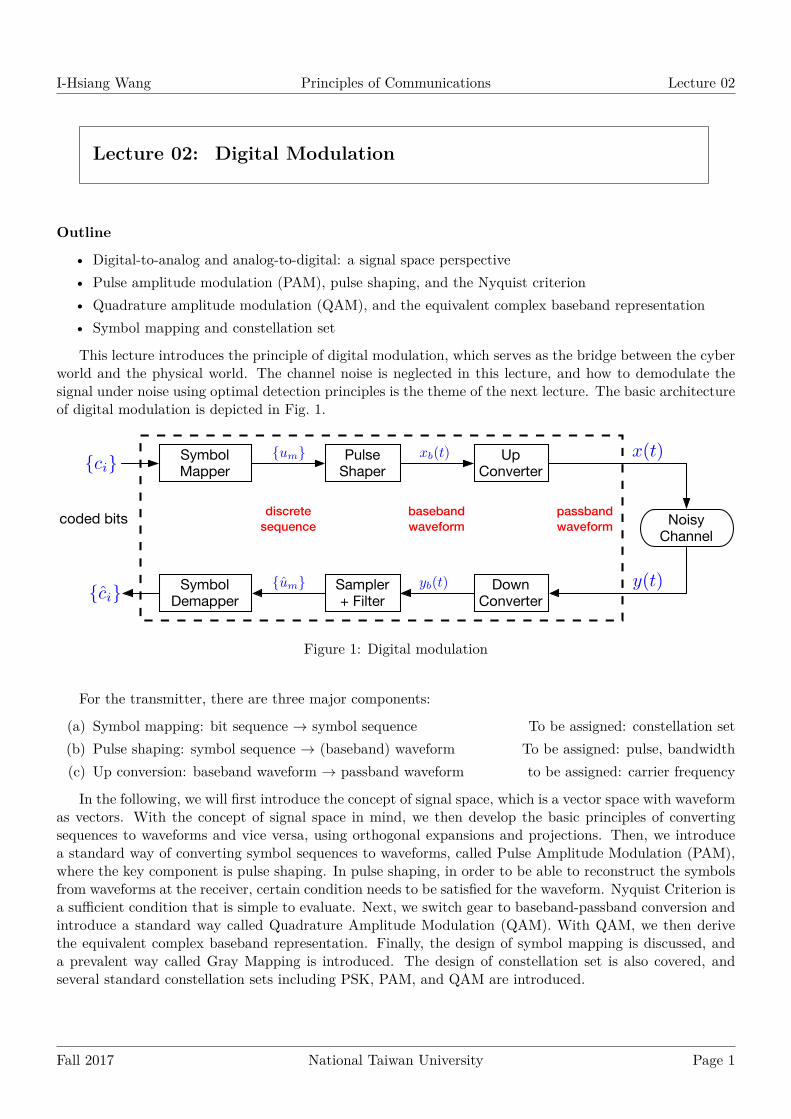
This lecture introduces the principle of digital modulation, which serves as the bridge between the cyberworld and the physical world. The channel noise is neglected in this lecture, and how to demodulate thesignal under noise using optimal detection principles is the theme of the next lecture. The basic architectureof digital modulation is depicted in Fig. 1.

passband waveform

Symbol Mapper

Pulse Shaper

Sampler + Filter

Symbol Demapper

discrete sequence

Up Converter

Down Converter

baseband waveform Noisy

Channelcoded bits

{ci}

{ci}

{um}

{um}

xb(t)

yb(t) y(t)

x(t)

Figure 1: Digital modulation

For the transmitter, there are three major components:

(a) Symbol mapping: bit sequence → symbol sequence To be assigned: constellation set(b) Pulse shaping: symbol sequence → (baseband) waveform To be assigned: pulse, bandwidth(c) Up conversion: baseband waveform → passband waveform to be assigned: carrier frequency

In the following, we will first introduce the concept of signal space, which is a vector space with waveformas vectors. With the concept of signal space in mind, we then develop the basic principles of convertingsequences to waveforms and vice versa, using orthogonal expansions and projections. Then, we introducea standard way of converting symbol sequences to waveforms, called Pulse Amplitude Modulation (PAM),where the key component is pulse shaping. In pulse shaping, in order to be able to reconstruct the symbolsfrom waveforms at the receiver, certain condition needs to be satisfied for the waveform. Nyquist Criterion isa sufficient condition that is simple to evaluate. Next, we switch gear to baseband-passband conversion andintroduce a standard way called Quadrature Amplitude Modulation (QAM). With QAM, we then derivethe equivalent complex baseband representation. Finally, the design of symbol mapping is discussed, anda prevalent way called Gray Mapping is introduced. The design of constellation set is also covered, andseveral standard constellation sets including PSK, PAM, and QAM are introduced.

Fall 2017 National Taiwan University


1 Prelude

From the discussions in Lecture 01, two key elements in digital communication systems can be identified:

(a) Conversion between bits and symbol sequences:• Source coding: quantization; table lookup• Channel coding: symbol mapper; symbol demapper

(b) Conversion between (discrete-time) sequences and (continuous-time) waveforms:• Source coding: sampling; interpolation filter• Channel coding: pulse shaping; sampling

This step builds the bridge between the cyber and the physical world and enables us to do things“digitally”.

We shall begin with the latter one: conversion between sequences and waveforms, and then come backto the former one later.

2 Signal space

2.1 Examples of conversion between sequences and waveforms

Recall from the course Signals and Systems, we have learned two approaches for the conversion betweensequences and waveforms:

• Fourier Series for time-limited signals {x(t), t ∈ T } where T is an interval with length T

• Sampling Theorem for band-limited signals {x(f) : −W ≤ f ≤ W}

The following table summarizes how to do analysis (from waveform to sequence) and synthesis (from sequenceto waveform). Recall that sinc(t) ≜ sin(πt)

πt .

Analysis (x(t) → x[m]) Synthesis (x[m] → x(t))

Fourier Series x[m] =1

T

∫Tx(t)e−

j2πmT

tdt x(t) =∞∑

m=−∞x[m]ej 2πm

Tt

Sampling Theorem x[m] = x(m 1

2W

)x(t) =

∞∑m=−∞

x[m] sinc(2Wt−m)

Table 1: Formulas of analysis and synthesis in Fourier Series and Sampling Theorem

The forms look similar. It turns out that such similarity is no coincidence, and there is an unifyingprinciple behind them. Such principle is called Signal Space, which can be viewed as an inner product spacewith waveforms identified as vectors. Below we briefly review vector space and inner product space. Formore details, please read Chapter 5 of [1].

2.2 Vector space and inner product space

Recall that a vector space (V,F) is a collection of vectors v ∈ V along with a set F of scalars, followingsome axioms. The scalar set F is usually the real field R or the complex field C. When the scalars are



constrained to be real, the corresponding vector space is called a real vector space. If the scalars arecomplex, the corresponding vector space is called a complex vector space. In the following, we focus oncomplex vector spaces, that is, the ambient scalar set F is C. When the context is clear, that is, the scalarfield is well-understood from the context, we often use V to denote the vector space.

A vector space follows some axioms (you can check your Linear Algebra textbook or Chapter 5 of [1]).One of the most important consequences is linearity:

∀α, β ∈ C, u,v ∈ V, αu+ βv ∈ V. (1)

Recall the following profound result from your Linear Algebra course.Theorem 1: For any finite-dimensional vector space V (that is, there exists a spanning set of V with finitecardinality), the following hold:

• If {v1, . . . ,vm} span V but are linearly dependent, then a subset of {v1, . . . ,vm} form a basis for Vwith n < m vectors.

• If {v1, . . . ,vm} are linearly independent but do not span V, then there exists a basis for V with n > mvectors that contains {v1, . . . ,vm}.

• Every basis of V has the same cardinality.

2.2.1 Inner product and norm

One of the most important kinds of vector space are Euclidean spaces Rn,Cn. The vectors here have thenatural notion of angle and length, which can be further abstracted into the concepts of inner product andnorm. An inner product ⟨·, ·⟩ on a complex vector space V satisfies the following axioms: for u,v,w ∈ Vand α, β ∈ C,

(a) Hermitian symmetry:⟨v,u⟩ = ⟨u,v⟩∗. (2)

(b) Hermitian bilinearity:⟨αu+ βv,w⟩ = α⟨u,w⟩+ β⟨v,w⟩. (3)

(c) Positivity:⟨v,v⟩ ≥ 0, with equality iff v = 0. (4)

A vector space with an inner product is called an inner product space. The norm ∥v∥ of a vector v isdefined as

∥v∥ ≜√⟨v,v⟩. (5)

In an inner product space, a set of vectors {ϕ1,ϕ2, . . .} is orthonormal if

⟨ϕi,ϕj⟩ =

{0 i = j

1 i = j. (6)

2.2.2 Projection

For an orthonormal basis Φ = {ϕi} of an inner product space V, the expansion of a vector v ∈ V overthe basis is fairly simple:

v =∑i

αiϕi, with αi = ⟨v,ϕi⟩. (7)

Furthermore, ∥v∥2 =∑

i|αi|2.More generally, we have a more general projection theorem as follows:



Theorem 2 (Projection): Consider a subspace S of an inner product space V and an orthonormal basisΦ of S. For any vector v ∈ V, there exists an unique v|S ∈ S such that ⟨v − v|S , s⟩ = 0 for all s ∈ S.Furthermore, this unique v|S is given as

v|S =∑i

αiϕi, with αi = ⟨v,ϕi⟩. (8)

Denoting v − v|S by v⊥S , we can see that any vector v can be decomposed into two orthogonal partsv⊥S and v|S , with v|S being the projection of v onto S.

2.3 Signal space point of view

Now, let us employ the linear algebraic point of view to interpret the two examples of conversion betweensequences and waveforms – Fourier Series and Sampling Theorem. First, we view a waveform u(t) as a vectorv and define the inner product between two waveforms as

⟨u,v⟩ ≜∫ ∞

−∞u(t)v∗(t)dt. (9)

For Fourier Series, we then identify the complex sinusoids as the basis (so-called Fourier Basis)

ϕm ≡ ϕm(t) ≜ 1√T

exp(j2πT mt), m ∈ Z, (10)

and rewrite the Fourier Series expansion as follows:

x[m] =

∫ ∞

−∞x(t)

1√Te−

j2πmT

t dt ≡ ⟨x,ϕm⟩ (11)

x ≡ x(t) =∞∑

m=−∞x[m]

1√Tej 2πm

Tt ≡

∑m

x[m]ϕm. (12)

Similarly for Sampling Theorem, we identify the uniformly shifted sinc functions as the basis (so-calledSinc Basis)

ϕm ≡ ϕm(t) ≜√2W sinc(2Wt−m), m ∈ Z, (13)

and rewrite Sampling Theorem as follows:

x[m] =1√2W

x(m/2W ) = {x(t) ∗√2W sinc(2Wt)}|t=m/2W =

∫ ∞

−∞x(t)

√2W sinc(2Wt−m)dt (14)

≡ ⟨x,ϕm⟩ (15)

x ≡ x(t) =

∞∑m=−∞

x(m/2W ) sinc(2Wt−m) =

∞∑m=−∞

x[m]ϕm(t) ≡∑m

x[m]ϕm. (16)

Exercise 1.

(a) Show that the Fourier Basis (10) and the Sinc Basis (13) are orthonormal.(b) Prove the last two equalities in equation (14).

As shown in the Exercise 1, both the Fourier Basis and the Sinc Basis are orthonormal bases. Hence,we can obtain a linear algebraic interpretation of analysis and sythesis of waveform signals:



• Synthesis can be viewed as expansion over an orthonormal basis:

{x[m]} → {ϕm(t)} → x(t) =

∞∑m=−∞

x[m]ϕm(t) (17)

• Analysis can be viewed as projection onto an orthonormal basis

x(t) → ϕm(t) → x[m] =

∫ ∞

−∞x(t)ϕ∗

m(t)dt. (18)

3 Pulse amplitude modulation (PAM)

With the signal space interpretation, we can see that for the conversion between sequences and waveformsin digital modulation, there are infinitely number of ways to select the orthonormal basis {ϕm(t),m ∈ Z}.On the other hand, a prevalent way in digital communication systems nowadays, is called Pulse AmplitudeModulation (PAM), where the basis consists of uniformly-time-shifted pulses:

ϕm(t) = p(t−mT ), T =1

2W, (19)

where T is called the transmission interval. T = 12W is determined by the operational bandwidth W ,

which will be made clear later.

3.1 PAM modulation – pulse shaping

PAM modulation follows the synthesis formula below (using the notation in the system diagram Fig. 1):

xb(t) =

∞∑m=−∞

um p(t−mT ). (20)

Hence, the above step is called pulse shaping.The pulse p(t) needs to be chosen carefully. From the point of view of the transmitter, ideally the

following properties are desirable:

(a) Time-limited: p(t) = 0 for all t < −τ with some finite τ > 0. This is because each symbol um arrives atthe modulator at some finite time, say mT − τ , so the contribution of um to the transmitted waveformxb(t) cannot start until mT − τ , which implies p(t) = 0 for t < −τ .

(b) Band-limited: p(f) = 0 for all |f | > Bb. Otherwise, the pulse easily violates physical constraints.1

Remark. It is impossible to make a pulse waveform p(t) “time-limited”and “band-limited”simultaneously.In practice, frequency-domain constraints are usually more stringent. Hence, we keep the property of beingband-limited but replace that of being time-limited by being approximately time-limited, that is, p(t) → 0rapidly as t → −∞. When we implement the pulse, usually the pulse p(t) is truncated, that is, the waveform is set to zero for all t < −τ for some τ ≥ 0. This truncation process will introduce additional errorand result in noise effectively. Hence, the faster p(t) → 0, the less noisy it will be.

1We use p(f) to denote the Fourier transform of p(t).



3.2 PAM demodulation – filtering + sampling

Although for modulation using an orthonormal basis, the optimal demodulation is to do projection asdiscussed in Section 2, in PAM we first filter the received signal by a filter q(t) and then sample the outputsignal at T -spaced sample times:

um =

∫ ∞

−∞yb(τ)q(mT − τ)dτ. (21)

Recall that in this lecture, we assume that there is no noise (that is, yb(t) = xb(t)), and hence the goalof the receiver is to ensure the reconstructed symbols um = um, ∀m. If this is satisfied, then we say thePAM system with pulse p(t) and filter q(t) is free of inter-symbol interference (ISI), that is, no aliasing effecthappens.

Since xb(t) =

∞∑k=−∞

uk p(t− kT ), by the linearity of convolution, we have

um = (xb ∗ q)(mT ) =∞∑

k=−∞uk g(mT − kT ) =

∞∑k=−∞

uk g((m− k)T )), (22)

where g(t) ≜ (p ∗ q)(t). Hence, a sufficient condition for um = um is

g(kT ) =

{0 if k = 0

1 if k = 0. (23)

Definition 3 (Ideal Nyquist): We say g(t) is ideal Nyquist with interval T if the above condition holds, thatis, g(kT ) = δk. In other words, if the pulse p(t) and the filter q(t) are chosen such that g(t) = (p ∗ q)(t) isideal Nyquist with interval T , then there is no inter-symbol interference (ISI), that is, the recovered um = umwhen yb(t) = xb(t).

Combined with the desired time-limited and band-limited properties of p(t), the desired properties forg(t) are summarized as follows:

(a) Time-limited: g(t) = 0 for all t < −τ with some finite τ > 0.Recall from the previous remark, we shall relax this criterion to approximately time-limited, that is,g(t) → 0 rapidly as t → −∞.

(b) Band-limited: g(f) = 0 for all |f | > Bb.(c) g(t) is ideal Nyquist with interval T .

3.3 Nyquist criterion

Let us introduce a simple equivalent condition in the frequency domain for checking the property of idealNyquist, as stated in the following theorem.Theorem 4 (Nyquist criterion): g(t) is ideal Nyquist with interval T if and only if its frequency domainresponse g(f) satisfies the following Nyquist Criterion:

T rect(Tf) =∑m

g(f − m

T

)rect(Tf), (24)

where the function

rect(f) ≜{1 |f | ≤ 1

2

0 otherwise. (25)



Proof The proof of this theorem is a simple application of the aliasing theorem. First, define

s(t) ≜∑m

g(mT ) sinc(

t

T−m

). (26)

Hence, g(t) is ideal Nyquist ⇐⇒ s(t) = sinc(tT

)⇐⇒ T rect(Tf) =

∑m

g(mT )e−j2πmTfT rect(Tf).

To complete the proof, it remains to show the following equality:∑m

g(f − m

T

)= T

∑m

g(mT )e−j2πmTf . (27)

Observing that the left-hand side (LHS) of (27) is the convolution of g(f) and the frequency domain impulsetrain

∑m δ(f −m/T ), we see the Inverse Fourier Transform (IFT) of the LHS of (27) is the multiplication

of the IFT of g(f) and the IFT of the impulse train:

g(t)

(T∑m

δ(t−mT )

)= T

∑m

g(mT )δ(t−mT ). (28)

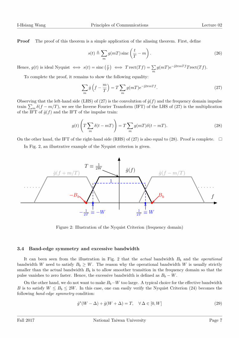
On the other hand, the IFT of the right-hand side (RHS) of (27) is also equal to (28). Proof is complete.In Fig. 2, an illustrative example of the Nyquist criterion is given.

g(f)

f

12T ≡ W− 1

2T ≡ −W

T ≡ 12W

g(f � m/T )g(f + m/T )

· · · · · ·· · · · · ·1

Figure 2: Illustration of the Nyquist Criterion (frequency domain)

3.4 Band-edge symmetry and excessive bandwidth

It can been seen from the illustration in Fig. 2 that the actual bandwidth Bb and the operationalbandwidth W need to satisfy Bb ≥ W . The reason why the operational bandwidth W is usually strictlysmaller than the actual bandwidth Bb is to allow smoother transition in the frequency domain so that thepulse vanishes to zero faster. Hence, the excessive bandwidth is defined as Bb −W .

On the other hand, we do not want to make Bb−W too large. A typical choice for the effective bandwidthB is to satisfy W ≤ Bb ≤ 2W . In this case, one can easily verify the Nyquist Criterion (24) becomes thefollowing band-edge symmetry condition:

g∗(W −∆) + g(W +∆) = T, ∀∆ ∈ [0,W ] (29)



which is equivalent to {Re {g(W −∆)}+ Re {g(W +∆)} = T

Im {g(W −∆)} = Im {g(W +∆)}, ∀∆ ∈ [0,W ] (30)

This can be proved by revoking the fact that both p(t) and q(t) are real-valued, and so does g(t). Theproof is left as an exercise. See the illustration in Fig. 3.

[� ]�

6.3.� THE�NYQUIST�CRITERION� 177�

Bb exceeds�Wb by�a�relatively�small�amount.� In�particular,�we�now�focus�on�the�case�where�Wb ≤ Bb < 2Wb.�

The� assumption�Bb < 2Wb means� that� g(f)� =� 0 for� |f | ≥ 2Wb.� Thus� for� 0�≤ f ≤ Wb,�g(f + 2mWb)�can�be�nonzero�only�for�m =�0�and�m =�−1.�Thus�the�Nyquist�criterion�(6.14)�in�this�positive�frequency�interval�becomes�

g(f) + g(f − 2Wb) = �T for� 0�≤ f ≤ Wb. (6.15)�

Since�p(t)�and�q(t)�are�real,�g(t)�is�also�real,�so�g(f−2Wb) = g∗(2Wb−f).� Substituting�this�in�(6.15)�and�letting�∆�=�f−Wb,�(6.15)�becomes�

T − g(Wb+∆)�=�g∗(Wb−∆). (6.16)�

This�is�sketched�and�interpreted�in�Figure�6.3.�The�figure�assumes�the�typical�situation�in�which�g(f)�is�real.� In�the�general�case,�the�figure�illustrates�the�real�part�of�g(f)�and�the�imaginary�part�satisfies�ℑ{g(Wb+∆)} =�ℑ{g(Wb−∆)}.�

g(f)�

T ✟✟✯

T − g(Wb−∆)�

f g(Wb+∆)✟✟✙

0� Wb Bb

Figure�6.3:� Band�edge�symmetry� illustrated� for�real� g(f):� For�each�∆,� 0≤∆≤Wb,�g(Wb+∆)�=�T − g(Wb−∆).� The�portion�of�the�curve�for�f ≥ Wb,�rotated�by�180o

around�the�point�(Wb, T/2),�is�equal�to�the�portion�of�the�curve�for�f ≤ Wb.�

Figure� 6.3�makes� it� particularly� clear� that�Bb must� satisfy�Bb ≥ Wb to� avoid� intersymbol�interference.� We� then� see� that� the� choice� of� g(f)� involves� a� tradeoff� between�making� g(f)�smooth,�so�as�to�avoid�a�slow�time�decay�in�g(t),�and�reducing�the�excess�of�Bb over�the�Nyquist�bandwidth�Wb.�This�excess�is�expressed�as�a�rolloff�factor11,�defined�to�be�(Bb/Wb)�− 1,�usually�expressed�as�a�percentage.�Thus�g(f)�in�the�figure�has�about�a�30%�rolloff.�

PAM filters in practice often have�raised�cosine�transforms.�The�raised�cosine�frequency�function,�for�any�given�rolloff�α between�0�and�1,�is�defined�by�

⎧�⎪⎨� 0�≤ |f | ≤ 1−α ;2TT,

πT ( 1−α 2α 2T

1+αcos2gα(f) = � )� , ;� (6.17)�T f |− 12−Tα ≤ |f | ≤ 2T

f | ≥ 1+α

| ⎪⎩�0, | 2T . 11The�requirement�for�a�small�rolloff�actually�arises�from�a�requirement�on�the�transmitted�pulse�p(t),�i.e., on �

the�actual�bandwidth�of�the�transmitted�channel�waveform,�rather�than�on�the�cascade�g(t) = �p(t)�∗ q(t).� The�tacit�assumption�here�is�that�p(f) = 0 when�g(f )�=�0.�One�reason�for�this�is�that�it�is�silly�to�transmit�energy�in�a�part�of�the�spectrum�that�is�going�to�be�completely�filtered�out�at�the�receiver.�We�see�later�that�p(f)�and�q(f)�are�usually�chosen�to�have�the�same�magnitude,�ensuring�that�p(f)�and�g(f)�have�the�same�rolloff.�

Cite as: Robert Gallager, course materials for 6.450 Principles of Digital Communications I, Fall 2006. MIT OpenCourseWare (http://ocw.mit.edu/), Massachusetts Institute of Technology. Downloaded on [DD Month YYYY].

T � Re{g(W � �)}

Re{g(W + �)}

Re{g(f)}

W

Figure 3: Illustration of band-edge symmetry (modifieded from Figure 6.3 of [1]).

Example 5 (Sinc pulse): The time-domain and frequency-domain representation of a sinc pulse is givenbelow:

g(t) = sinc(

t

T

), (31)

g(f) = T rect(fT ). (32)

The operational bandwidth W is equal to the actual bandwidth Bb.Example 6 (Raised cosine pulse): The time-domain and frequency-domain representation of a raised cosinepulse is given below

gβ(t) =

π4 sinc

(12β

), if |f | = T

2β

sinc(tT

) cos(πβtT

)

1−4β2t2

T2

, otherwise(33)

gβ(f) =

T if |f | ≤ 1−β

2T

0 if |f | > 1+β2T

T cos2(πT2β (|f | −1−β2T )) if 1−β

2T < |f | ≤ 1+β2T

(34)

The excessive bandwidth Bb −W = (1 + β)W −W = βW is parameterized by β ∈ [0, 1], called the rollofffactor. The larger it is, the smoother it transits from T to 0 in the frequency domain, and hence convergesto zero faster in the time domain. In practice, rolloffs as sharp as 5% to 10% is used.Remark. Engineers often define the rolloff factor as Bb

W − 1.

You can easily check that both the sinc pulse and the raised cosine pulse satisfy the band-edge symmetrycondition (29). This is left as an exercise.Exercise 2.

(a) Prove the band-edge symmetry condition (29) for real g(t) when W ≤ Bb ≤ 2W .(b) Check the Fourier transform of the raised cosine pulse gβ(t) in (33) is indeed the gβ(f) in (34).



(c) Check that the raised cosine pulse satisfy the band-edge symmetry condition and hence ideal Nyquistwith interval T .

(d) Show that the sinc pulse converges to 0 as t → ∞ in the order of 1/t, while the raised cosine pulseconverges to zero in the order of 1/t3.

3.5 Choosing {p(t−mT )} as an orthonormal set

Now we have seen the desired properties of g(t) ≜ (p ∗ q)(t): approximately time-limited, band-limited,and ideal Nyquist with interval T . Earlier in Section 2, we also demonstrated the effectiveness of usingthe waveform expansion over and projection onto an orthonormal basis of a signal space to interpret theconversion between sequences and waveforms. What remains in this section, is to show that for the T -spaceshifted pulses {p(t−mT )}, it forms an orthonormal basis if and only if |p(f)|2 satisfy the Nyquist criterion.

Let us begin with some simple observations. Since g(f) = p(f)q(f), we can simply choose |p(f)| =|q(f)| =

√g(f). With this choice, we have the following nice theorem relating ISI-free condition and

orthogonality:Theorem 7: Suppose g(f) = |p(f)|2 and satisfies the Nyquist Criterion with interval T . Then, {p(t−mT ) :m ∈ Z} form an orthonormal set. Conversely, if {p(t−mT ) : m ∈ Z} form an orthonormal set, then |p(f)|2satisfies the Nyquist Criterion.

Proof To make g(f) = |p(f)|2, we need to choose q(f) = p∗(f) ⇐⇒ q(t) = p∗(−t). Plugging ing(t) = (p ∗ q)(t), we get

g(kT ) =

∫ ∞

−∞p(t)p∗(−kT + t)dt =

∫ ∞

−∞p(t)p∗(t− kT )dt. (35)

If g(t) is ideal Nyquist with interval T , then we can conclude that

⟨p(t−mT ), p(t− nT )⟩ =∫ ∞

−∞p(t−mT )p∗(t−nT )dt =

∫ ∞

−∞p(τ)p∗(τ − (n−m)T )dτ =

{1 n = m

0 n = m. (36)

Conversely, if {p(t−mT )} form an orthonormal set, we can show that g(kT ) = 1 if and only if k = 0 usinga similar calculation. Proof complete.

Summary To sum up, for PAM modulation and demodulation, the following principles are usually usedfor the design of the pulse p(t) at the transmitter and the corresponding filter q(t) at the receiver:

(a) p(f) = q∗(f) (phase offset)(b) |p(f)|2 satisfies the Nyquist Criterion(c) If p(t) ∈ R (which is normally the case), then q(f) = p∗(f) = p(−f) and hence q(t) = p(−t).(d) For faster decay in the time-domain (less approximation error) in t =⇒ need “larger room” for

smoother transition from T to 0 in the frequency-domainExercise 3. Implement and simulate a PAM modulator/demodulator for the ideal baseband channel yb(t) =xb(t) using raised cosine pulses in your computer.



4 Quadrature amplitude modulation (QAM)

4.1 QAM modulation

In many communication systems, the transmitted signals have to obey certain constraints in the fre-quency domain and can only occupy a certain passband frequency band. Hence, at the transmitter it isnecessary to convert the baseband signal to a passband signal. In this course, we introduce a widely usedapproach called quadrature amplitude modulation (QAM), which is essentially a combination of two indi-vidual branches of PAM waveforms, say, x(I)b (t) and x

(Q)b (t). One branch is mixed with a cosine waveform

with center frequency fc, while the other is mixed with a sine waveform with the same center frequency:

x(t) = x(I)b (t)

√2 cos(2πfct)− x

(Q)b (t)

√2 sin(2πfct) (37)

By defining a complex baseband waveform

xb(t) ≜ x(I)b (t) + jx(Q)

b (t), (38)

we have an equivalent representation for the passband signal:

x(t) =√2Re {xb(t) exp(j2πfct)} . (39)

Conventionally, x(I)b (t) and x

(Q)b (t) are called the in-phase part and the quadrature part of the complex

basedband waveform xb(t).

Recall that both x(I)b (t) and x

(Q)b (t) are PAM waveforms:

x(I)b (t) =

∑m

u(I)m p(t−mT ) (40)

x(Q)b (t) =

∑m

u(Q)m p(t−mT ) (41)

and hence the complex basedband waveform

xb(t) =∑m

um p(t−mT ), (42)

where um ≜ u(I)m + ju(Q)

m ∈ C is a complex symbol.In words, the QAM modulation can be viewed purely in the complex domain and the equivalent real-

domain implementation, as illustrated in Fig. 4. The mixing with the complex sinusoid√2 exp(j2πfct) (or

the mixing with the cosine/sine waveforms in the real-domain implementation) is called up-conversion.

4.2 QAM demodulation

As for the QAM demodulation, one should split the received signal y(t) into two branches. One branchaims to reconstruct the in-phase symbol sequence, while the other aims to reconstruct the quadrature part.For the in-phase part, the received signal is first multiplied by the cosine waveform

√2 cos(2πfct), low-pass

filtered with one-sided bandwidth Bb, filtered by q(t), and then uniformly sampled with interval T . For thequadrature part, the received signal is first multiplied by the sine waveform −

√2 sin(2πfct), low-pass filtered

with one-sided bandwidth Bb, filtered by q(t), and then uniformly sampled with interval T . The mixingof the passband signal with cosine and the sine waveforms followed by low-pass filtering with one-sidedbandwidth Bb is called down-conversion. Note that the concatenation of the low-pass filter rect( f

2Bb) and

the PAM demodulation filter q(f) is always equal to q(f). Hence, these two blocks can be merged into one.See Fig. 5 for an illustration.



PAMp(t)

�2 cos(2�fct)

PAMp(t)

��

2 sin(2�fct)

{u(Q)m }

{u(I)m }

x(I)b (t)

x(Q)b (t)

x(t)

(a) Real-domain implementation

PAMp(t)

x(t){um}xb(t)

�2 exp(j2�fct)

Re{·}

(b) Equivalent complex baseband model

Figure 4: QAM modulation: PAM modulations + up-conversion



y(t)

�2 cos(2�fct)

��

2 sin(2�fct)

Filterq(t)

Filterq(t)

T = 12W

T = 12W

{u(Q)m }

{u(I)m }LPF

1 {|f | ≤ Bb}

LPF1 {|f | ≤ Bb}

y(I)b (t)

y(Q)b (t)

(a) Real-domain implementation

y(t) Step Filter1 {f ≥ 0}

yb(t)

�2 exp(�j2�fct)

Filterq(t)

T = 12W

{um}

(b) Equivalent complex-domain implementation

y(t)

�2 cos(2�fct)

��

2 sin(2�fct)

Filterq(t)

Filterq(t)

T = 12W

T = 12W

{u(Q)m }

{u(I)m }

(c) Simplified implementation

Figure 5: QAM demodulation: down-conversion + PAM demodulations



Exercise 4. Show that in the equivalent complex-domain implementation of QAM demodulation in Fig. 5(b),the complex baseband signal yb(t) is indeed equal to

y(I)b (t) + jy(Q)

b (t). (43)

References

[1] R. G. Gallager, Principles of Digital Communication. Cambridge University Press, 2008.


lecture 02: digital modulation -...

Documents