logic for computer science - lab for automated reasoning and
TRANSCRIPT
Logic for Computer Science
Harald Ganzinger
Summer Term 2002
Logic in Computer Science 2
computation is deduction
• logic programming, relational data bases• operational semantics of PLs
proof theory
• mathematics on the computer• constructive proofs and program synthesis
axiomatized domains
• modelling in logic• knowledge representation• specification and verification• rapid prototyping
descriptive complexity theory
Emphasis in this Course 3
• introduction into logics and deductive services underlying important
domains of application
– first-order logic (universal calculus; theorem proving)– Horn clause logic (logic programming; goal solving)– temporal logic (verification of communicating programs; model
checking)– [typed λ-calculus (constructive proofs; program extraction)]
• proof systems: soundness, completeness, complexity, implementation
• efficient algorithms for specific deduction problems
• exercises: implementation (in SML) of theoretical constructions
Literature 4
Schoning: Logik fur Informatiker, Spektrum
Fitting: First-Order Logic and Automated Theorem Proving, Springer
Huth, Ryan: Logic in Computer Science: Modelling and reasoning about
systems, Cambridge University Press
Gallier: Logic for Computer Science, Harper & Row
Reeves, Clarke: Logic for Computer Science, Addison-Wesley
Ben-Ari: Mathematical Logic for Computer Science, Prentice Hall
Sperschneider, Antoniou: Logic, a Foundation for Computer Science
de Swart et al: Logic: Mathematics, Language, Computer Science and
Philosophy, Vol. II: Logic and Computer Science, Peter Lang
Part 1: First-Order Logic 5
• formalizes fundamental mathematical concepts
• expressive (Turing-complete)
• not too expressive (not axiomatizable: natural numbers, uncountable
sets)
• rich structure of decidable fragments
• rich model and proof theory
First-order logic is also called (first-order) predicate logic.
1.1 Syntax 6
• non-logical symbols (domain-specific)
⇒ terms, atomic formulas
• logical symbols (domain-independent)
⇒ Boolean combinations, quantifiers
Signature 7
Usage: fixing the alphabet of non-logical symbols
Σ = (Ω,Π),
where
• Ω a set of function symbols f with arity n ≥ 0, written f/n,
• Π a set of predicate symbols p with arity m ≥ 0, written p/m.
If n = 0 then f is also called a constant (symbol). If m = 0 then p is also
called a propositional variable. We use letters P , Q, R, S, to denote
propositional variables.
Refined concept for practical applications: many-sorted signatures
(corresponds to simple type systems in programming languages); not so
interesting from a logical point of view
Variables 8
Predicate logic admits the formulation of abstract, schematic assertions.
(Object) variables are the technical tool for schematization.
We assume that
X
is a given countably infinite set of symbols which we use for (the
denotation of) variables.
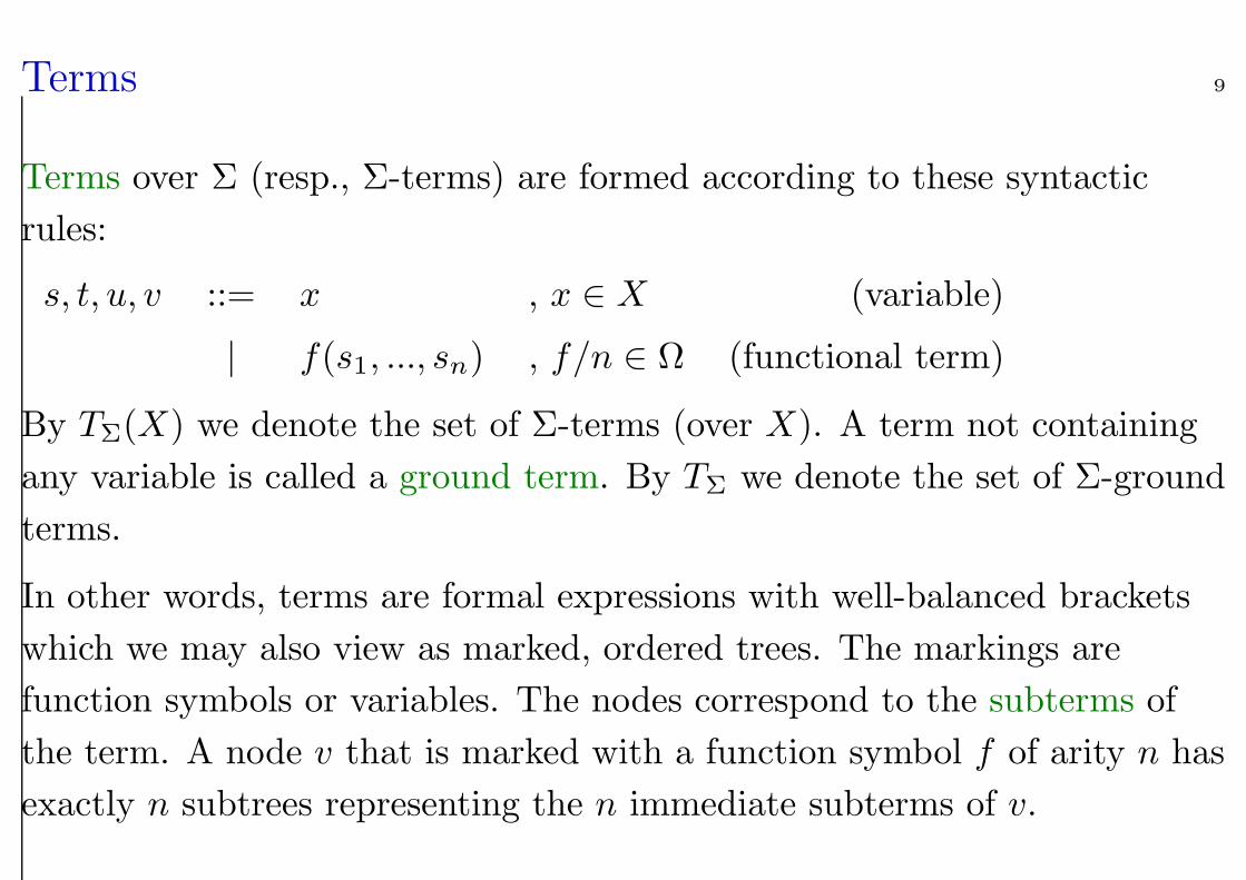
Terms 9
Terms over Σ (resp., Σ-terms) are formed according to these syntactic
rules:
s, t, u, v ::= x , x ∈ X (variable)
| f(s1, ..., sn) , f/n ∈ Ω (functional term)
By TΣ(X) we denote the set of Σ-terms (over X). A term not containing
any variable is called a ground term. By TΣ we denote the set of Σ-ground
terms.
In other words, terms are formal expressions with well-balanced brackets
which we may also view as marked, ordered trees. The markings are
function symbols or variables. The nodes correspond to the subterms of
the term. A node v that is marked with a function symbol f of arity n has
exactly n subtrees representing the n immediate subterms of v.
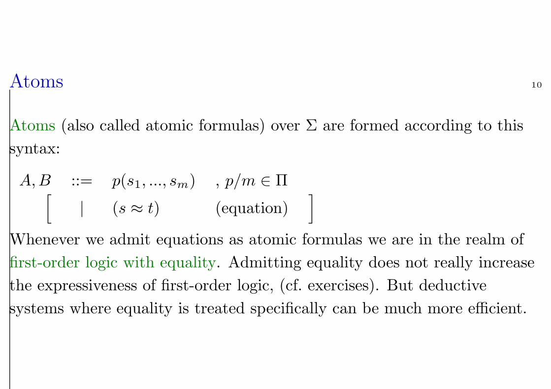
Atoms 10
Atoms (also called atomic formulas) over Σ are formed according to this
syntax:
A,B ::= p(s1, ..., sm) , p/m ∈ Π[
| (s ≈ t) (equation)]
Whenever we admit equations as atomic formulas we are in the realm of
first-order logic with equality. Admitting equality does not really increase
the expressiveness of first-order logic, (cf. exercises). But deductive
systems where equality is treated specifically can be much more efficient.
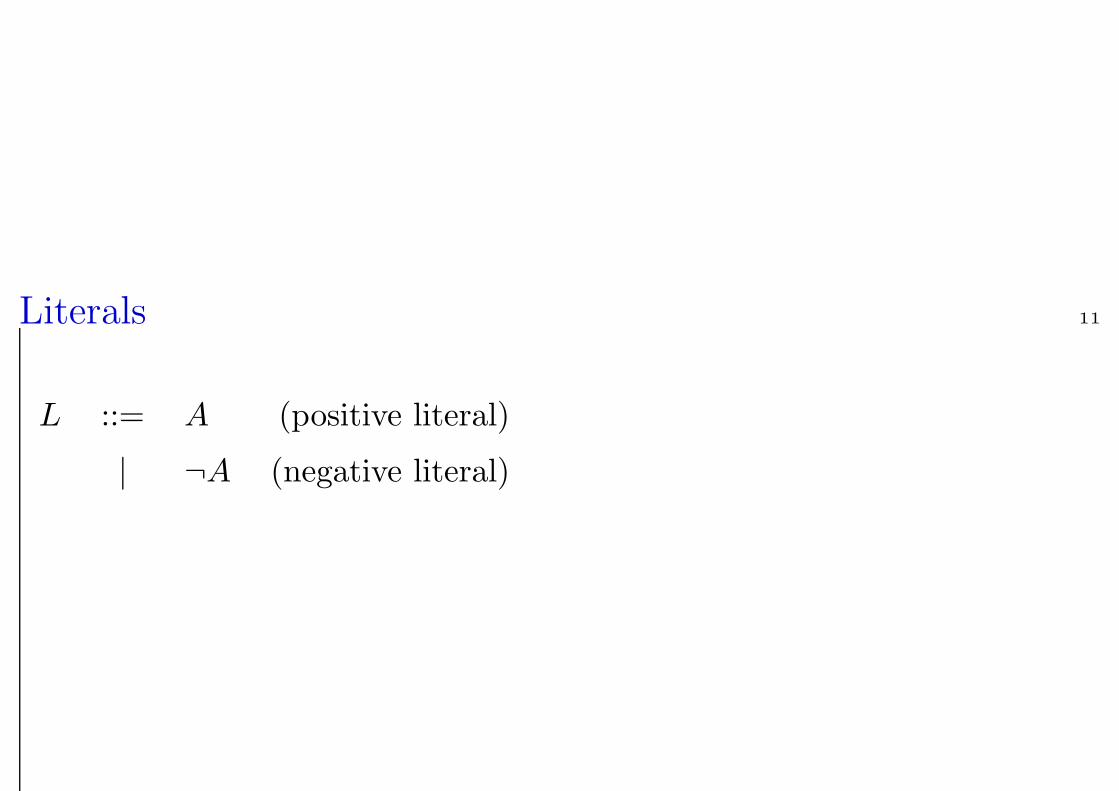
Literals 11
L ::= A (positive literal)
| ¬A (negative literal)
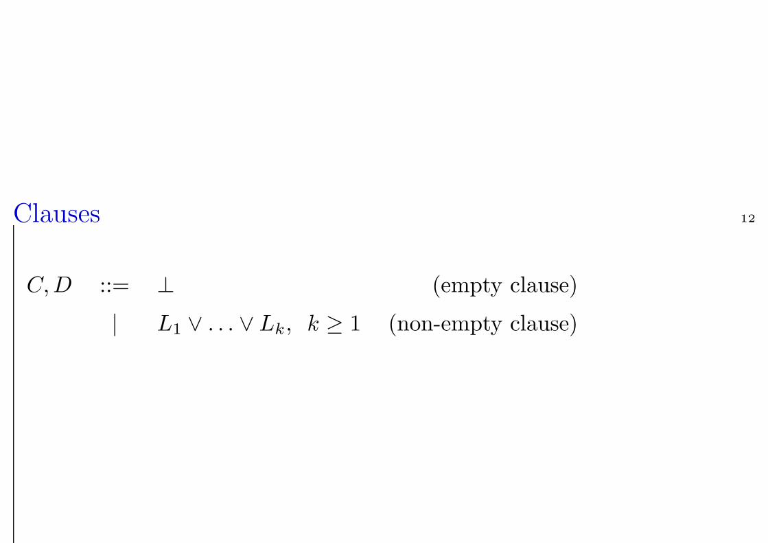
Clauses 12
C,D ::= ⊥ (empty clause)
| L1 ∨ . . . ∨ Lk, k ≥ 1 (non-empty clause)
General First-Order Formulas 13
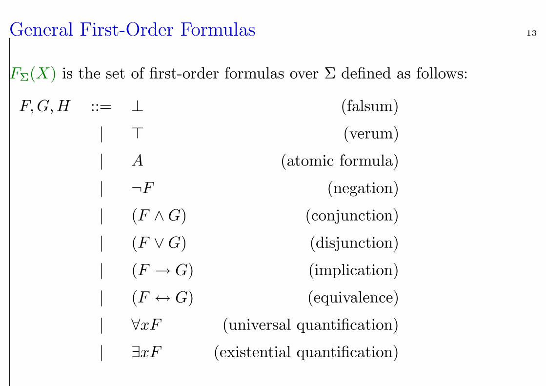
FΣ(X) is the set of first-order formulas over Σ defined as follows:
F,G,H ::= ⊥ (falsum)
| > (verum)
| A (atomic formula)
| ¬F (negation)
| (F ∧G) (conjunction)
| (F ∨G) (disjunction)
| (F → G) (implication)
| (F ↔ G) (equivalence)
| ∀xF (universal quantification)
| ∃xF (existential quantification)
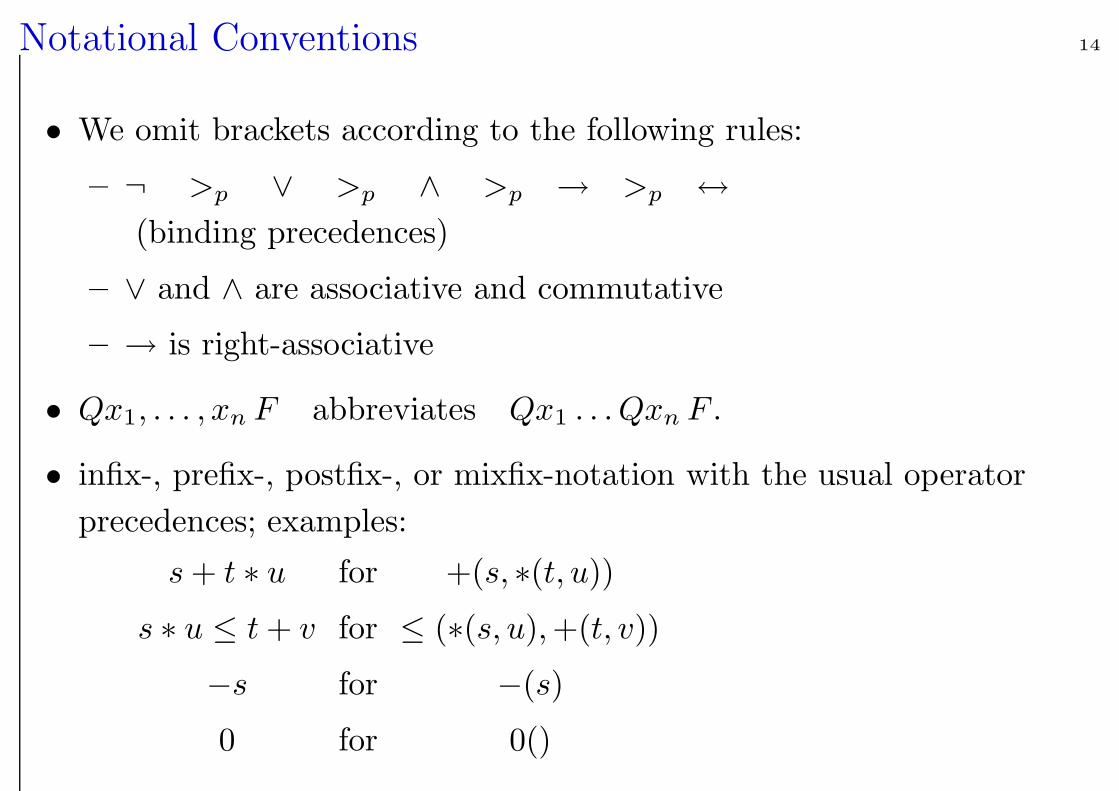
Notational Conventions 14
• We omit brackets according to the following rules:
– ¬ >p ∨ >p ∧ >p → >p ↔
(binding precedences)
– ∨ and ∧ are associative and commutative
– → is right-associative
• Qx1, . . . , xn F abbreviates Qx1 . . . Qxn F .
• infix-, prefix-, postfix-, or mixfix-notation with the usual operator
precedences; examples:
s + t ∗ u for +(s, ∗(t, u))
s ∗ u ≤ t + v for ≤ (∗(s, u),+(t, v))
−s for −(s)
0 for 0()
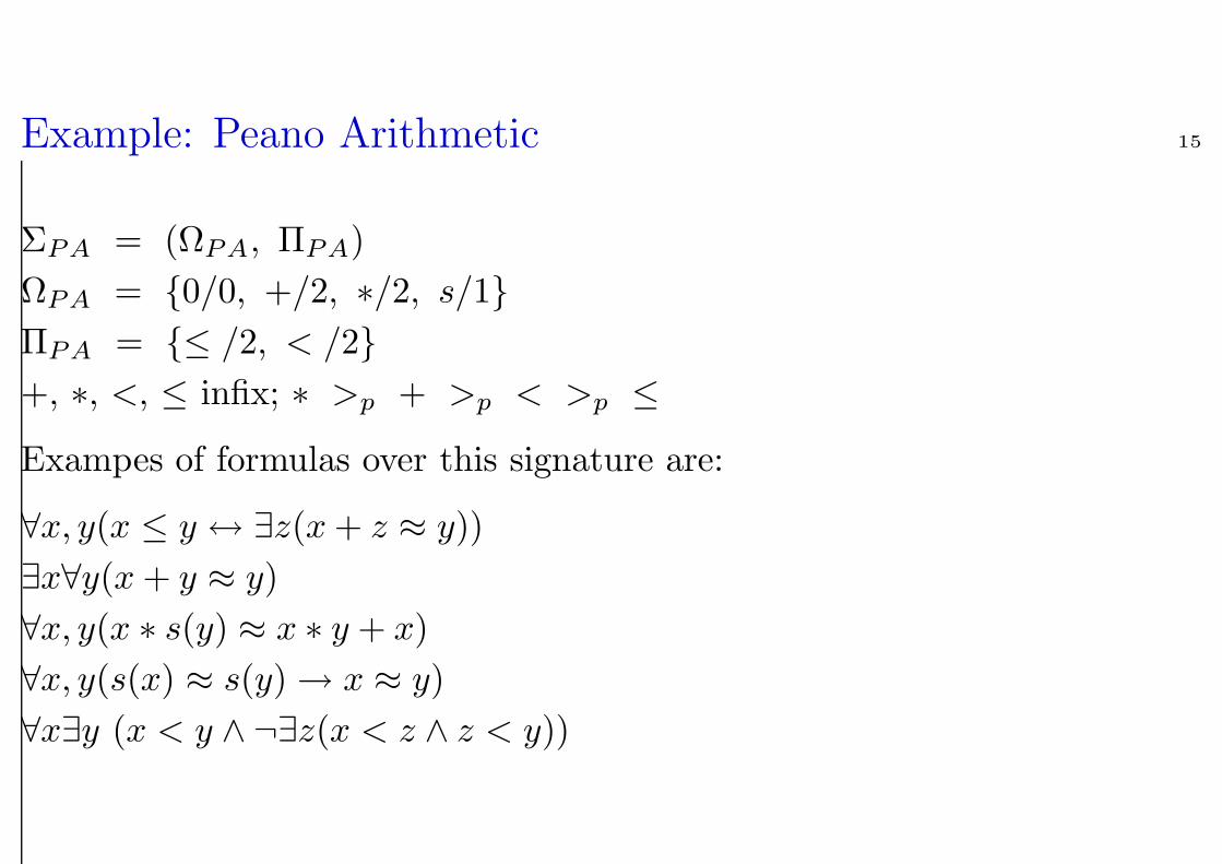
Example: Peano Arithmetic 15
ΣPA = (ΩPA, ΠPA)
ΩPA = 0/0, +/2, ∗/2, s/1
ΠPA = ≤ /2, < /2
+, ∗, <, ≤ infix; ∗ >p + >p < >p ≤
Exampes of formulas over this signature are:
∀x, y(x ≤ y ↔ ∃z(x + z ≈ y))
∃x∀y(x + y ≈ y)
∀x, y(x ∗ s(y) ≈ x ∗ y + x)
∀x, y(s(x) ≈ s(y)→ x ≈ y)
∀x∃y (x < y ∧ ¬∃z(x < z ∧ z < y))
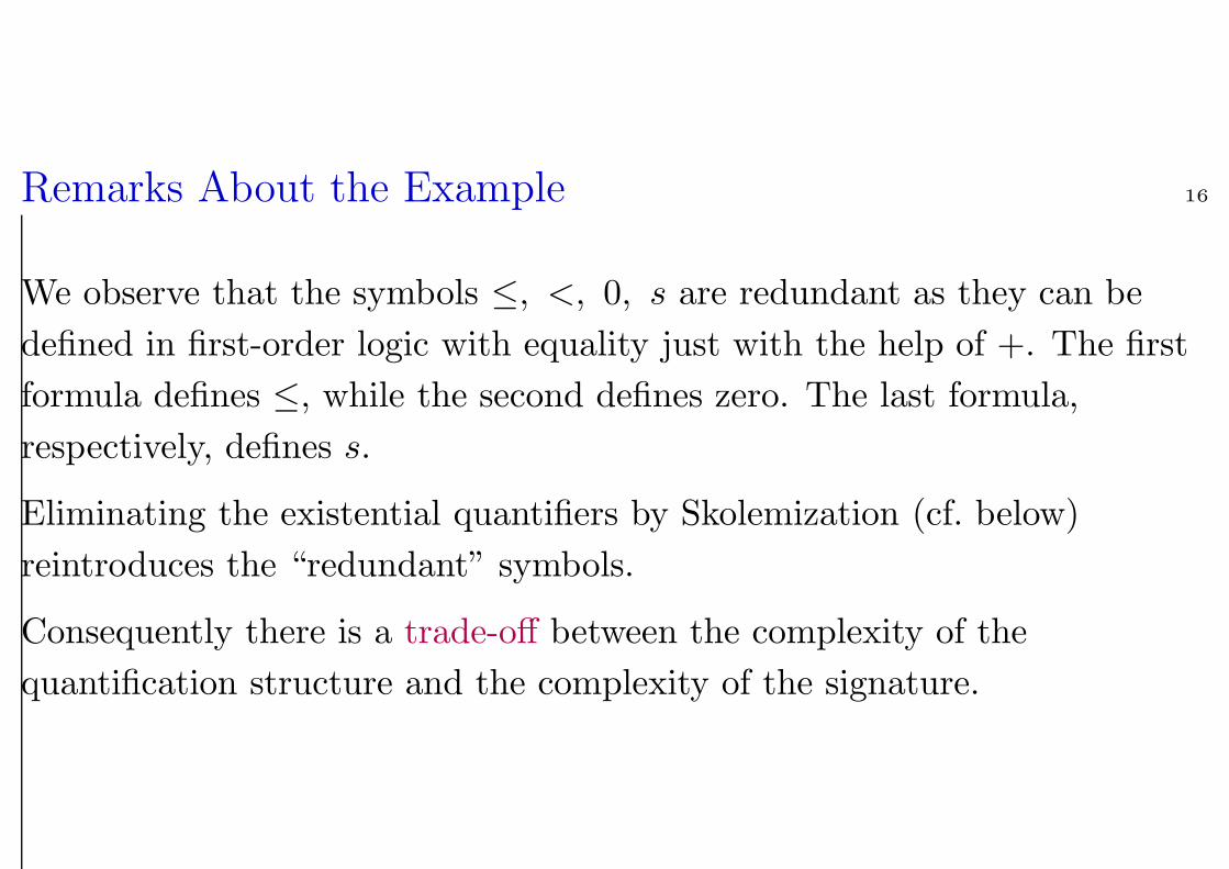
Remarks About the Example 16
We observe that the symbols ≤, <, 0, s are redundant as they can be
defined in first-order logic with equality just with the help of +. The first
formula defines ≤, while the second defines zero. The last formula,
respectively, defines s.
Eliminating the existential quantifiers by Skolemization (cf. below)
reintroduces the “redundant” symbols.
Consequently there is a trade-off between the complexity of the
quantification structure and the complexity of the signature.
Bound and Free Variables 17
In QxF, Q ∈ ∃, ∀, we call F the scope of the quantifier Qx. An
occurrence of a variable x is called bound, if it is inside the scope of a
quantifier Qx. Any other occurrence of a variable is called free.
Formulas without free variables are also called closed formulas or
sentential forms.
Formulas without variables are called ground.
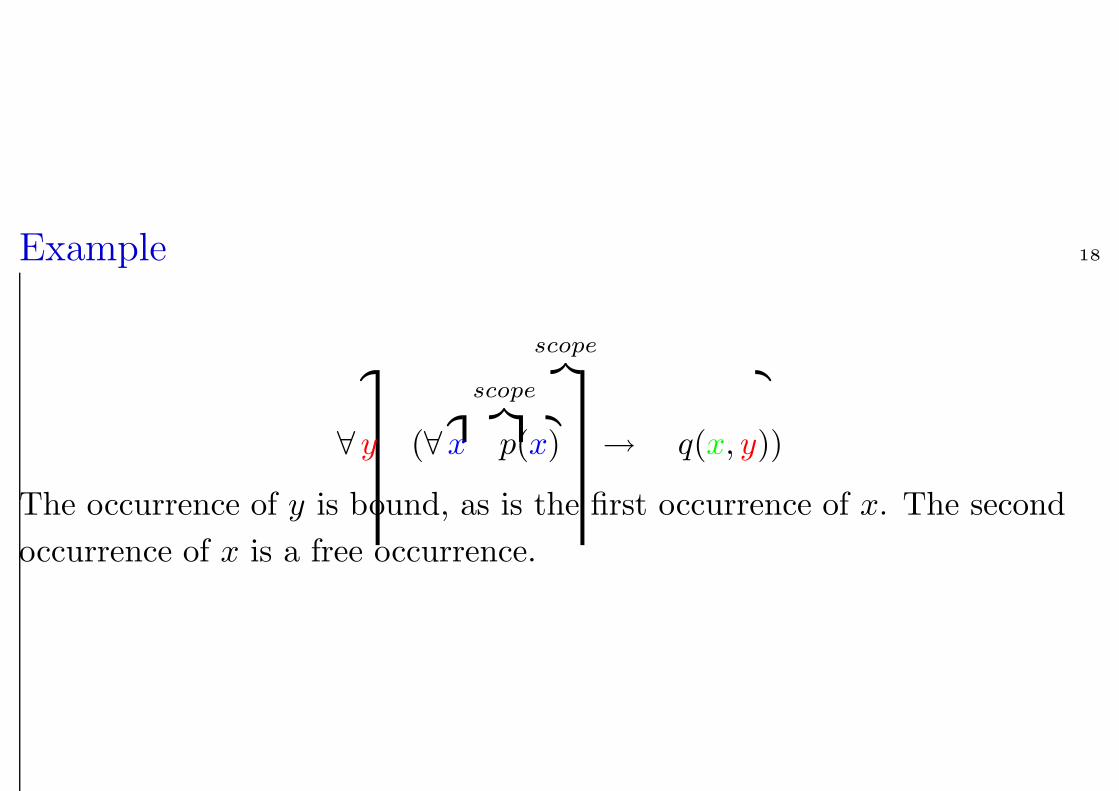
Example 18
∀
scope︷ ︸︸ ︷
y (∀
scope︷ ︸︸ ︷
x p(x) → q(x, y))
The occurrence of y is bound, as is the first occurrence of x. The second
occurrence of x is a free occurrence.
Substitutions 19
Substitution is a fundamental operation on terms and formulas that occurs
in all inference systems for first-order logic. In the presence of
quantification it is surprisingly complex.
By F [s/x] we denote the result of substituting all free occurrences of x in
F by the term s.
Formally we define F [s/x] by structural induction over the syntactic
structure of F by the equations depicted on the next page.
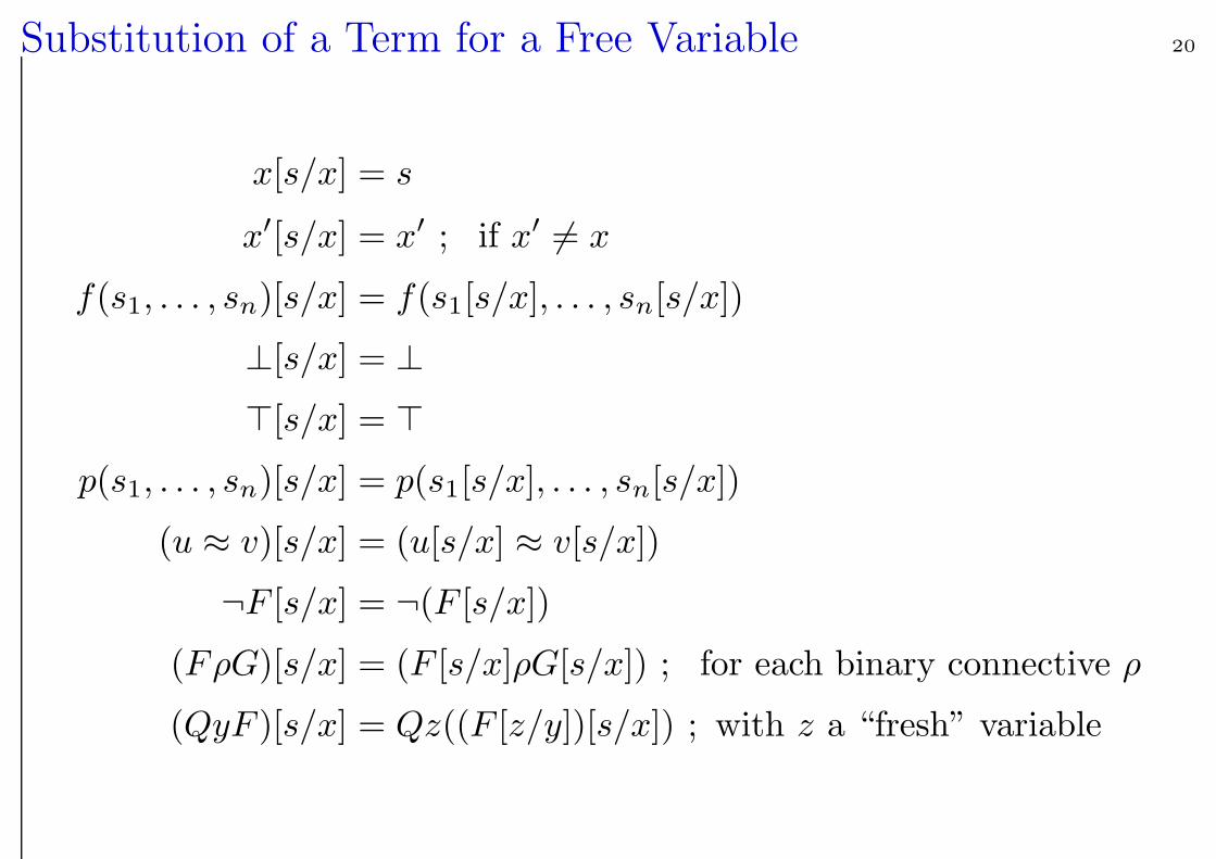
Substitution of a Term for a Free Variable 20
x[s/x] = s
x′[s/x] = x′ ; if x′ 6= x
f(s1, . . . , sn)[s/x] = f(s1[s/x], . . . , sn[s/x])
⊥[s/x] = ⊥
>[s/x] = >
p(s1, . . . , sn)[s/x] = p(s1[s/x], . . . , sn[s/x])
(u ≈ v)[s/x] = (u[s/x] ≈ v[s/x])
¬F [s/x] = ¬(F [s/x])
(FρG)[s/x] = (F [s/x]ρG[s/x]) ; for each binary connective ρ
(QyF )[s/x] = Qz((F [z/y])[s/x]) ; with z a “fresh” variable
Why Substitution is Complicated 21
We need to make sure that the (free) variables in s are not captured upon
placing s into the scope of a quantifier, hence the renaming of the bound
variable y into a “fresh”, that is, previously unused, variable z.
Why this definition of substitution is well-defined will be discussed below.
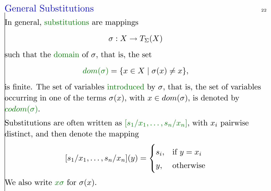
General Substitutions 22
In general, substitutions are mappings
σ : X → TΣ(X)
such that the domain of σ, that is, the set
dom(σ) = x ∈ X | σ(x) 6= x,
is finite. The set of variables introduced by σ, that is, the set of variables
occurring in one of the terms σ(x), with x ∈ dom(σ), is denoted by
codom(σ).
Substitutions are often written as [s1/x1, . . . , sn/xn], with xi pairwise
distinct, and then denote the mapping
[s1/x1, . . . , sn/xn](y) =
si, if y = xi
y, otherwise
We also write xσ for σ(x).
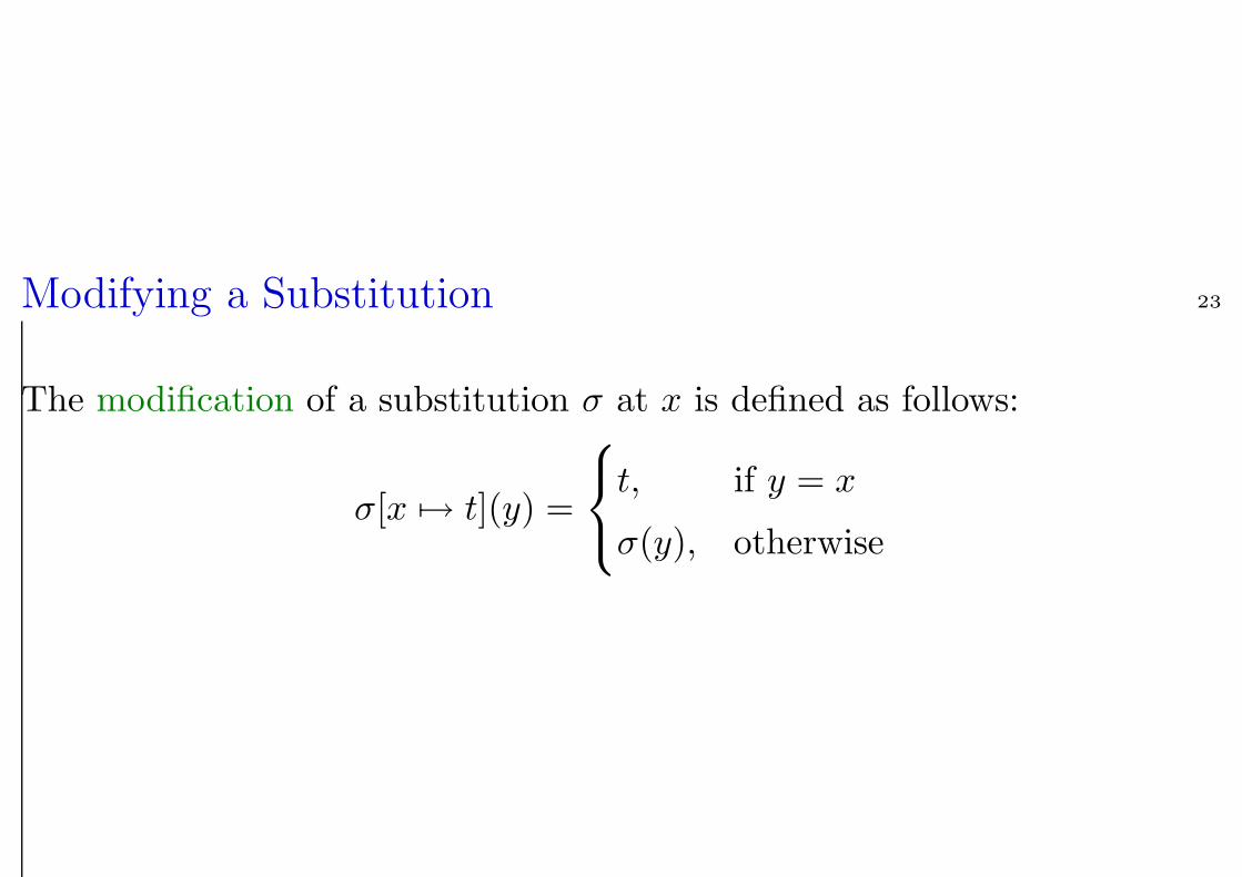
Modifying a Substitution 23
The modification of a substitution σ at x is defined as follows:
σ[x 7→ t](y) =
t, if y = x
σ(y), otherwise
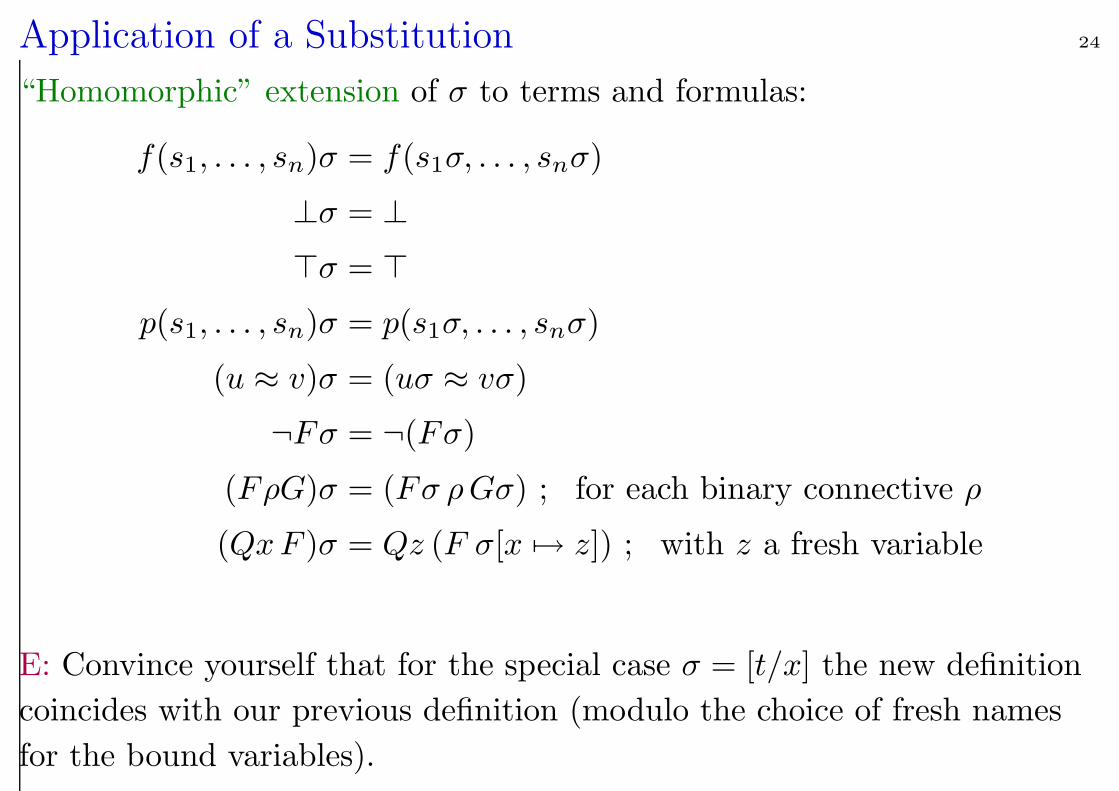
Application of a Substitution 24
“Homomorphic” extension of σ to terms and formulas:
f(s1, . . . , sn)σ = f(s1σ, . . . , snσ)
⊥σ = ⊥
>σ = >
p(s1, . . . , sn)σ = p(s1σ, . . . , snσ)
(u ≈ v)σ = (uσ ≈ vσ)
¬Fσ = ¬(Fσ)
(FρG)σ = (Fσ ρGσ) ; for each binary connective ρ
(QxF )σ = Qz (F σ[x 7→ z]) ; with z a fresh variable
E: Convince yourself that for the special case σ = [t/x] the new definition
coincides with our previous definition (modulo the choice of fresh names
for the bound variables).
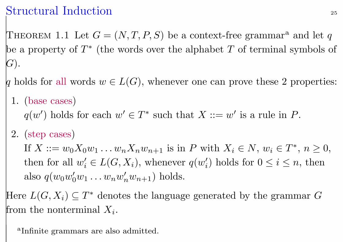
Structural Induction 25
Theorem 1.1 Let G = (N,T, P, S) be a context-free grammara and let q
be a property of T ∗ (the words over the alphabet T of terminal symbols of
G).
q holds for all words w ∈ L(G), whenever one can prove these 2 properties:
1. (base cases)
q(w′) holds for each w′ ∈ T ∗ such that X ::= w′ is a rule in P .
2. (step cases)
If X ::= w0X0w1 . . . wnXnwn+1 is in P with Xi ∈ N , wi ∈ T ∗, n ≥ 0,
then for all w′i ∈ L(G,Xi), whenever q(w′
i) holds for 0 ≤ i ≤ n, then
also q(w0w′0w1 . . . wnw′
nwn+1) holds.
Here L(G,Xi) ⊆ T ∗ denotes the language generated by the grammar G
from the nonterminal Xi.
aInfinite grammars are also admitted.
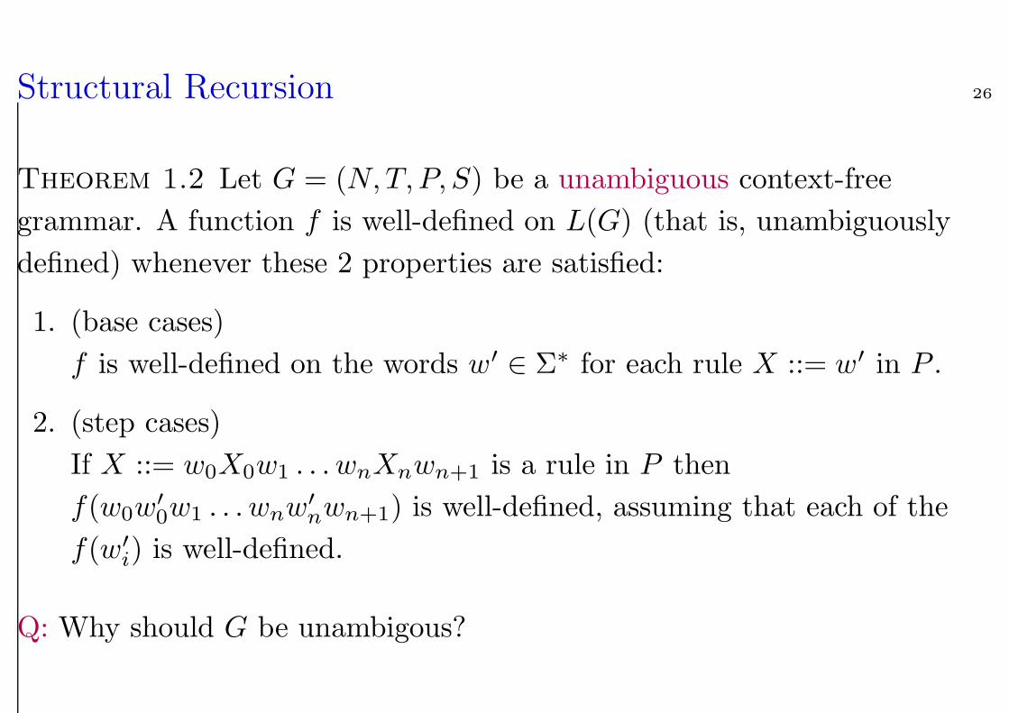
Structural Recursion 26
Theorem 1.2 Let G = (N,T, P, S) be a unambiguous context-free
grammar. A function f is well-defined on L(G) (that is, unambiguously
defined) whenever these 2 properties are satisfied:
1. (base cases)
f is well-defined on the words w′ ∈ Σ∗ for each rule X ::= w′ in P .
2. (step cases)
If X ::= w0X0w1 . . . wnXnwn+1 is a rule in P then
f(w0w′0w1 . . . wnw′
nwn+1) is well-defined, assuming that each of the
f(w′i) is well-defined.
Q: Why should G be unambigous?
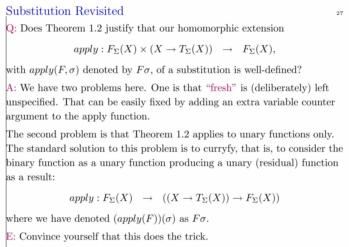
Substitution Revisited 27
Q: Does Theorem 1.2 justify that our homomorphic extension
apply : FΣ(X)× (X → TΣ(X)) → FΣ(X),
with apply(F, σ) denoted by Fσ, of a substitution is well-defined?
A: We have two problems here. One is that “fresh” is (deliberately) left
unspecified. That can be easily fixed by adding an extra variable counter
argument to the apply function.
The second problem is that Theorem 1.2 applies to unary functions only.
The standard solution to this problem is to curryfy, that is, to consider the
binary function as a unary function producing a unary (residual) function
as a result:
apply : FΣ(X) → ((X → TΣ(X))→ FΣ(X))
where we have denoted (apply(F ))(σ) as Fσ.
E: Convince yourself that this does the trick.
1.2. Semantics 28
To give semantics to a logical system means to define a notion of truth for
the formulas. The concept of truth that we will now define for first-order
logic goes back to Tarski.
In classical logic (dating back to Aristoteles) there are “only” two truth
values “true” and “false” which we shall denote, respectively, by 1 and 0.
There are multi-valued logics having more than two truth values.
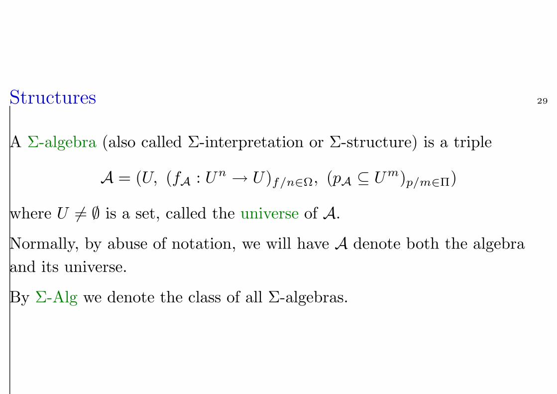
Structures 29
A Σ-algebra (also called Σ-interpretation or Σ-structure) is a triple
A = (U, (fA : Un → U)f/n∈Ω, (pA ⊆ Um)p/m∈Π)
where U 6= ∅ is a set, called the universe of A.
Normally, by abuse of notation, we will have A denote both the algebra
and its universe.
By Σ-Alg we denote the class of all Σ-algebras.
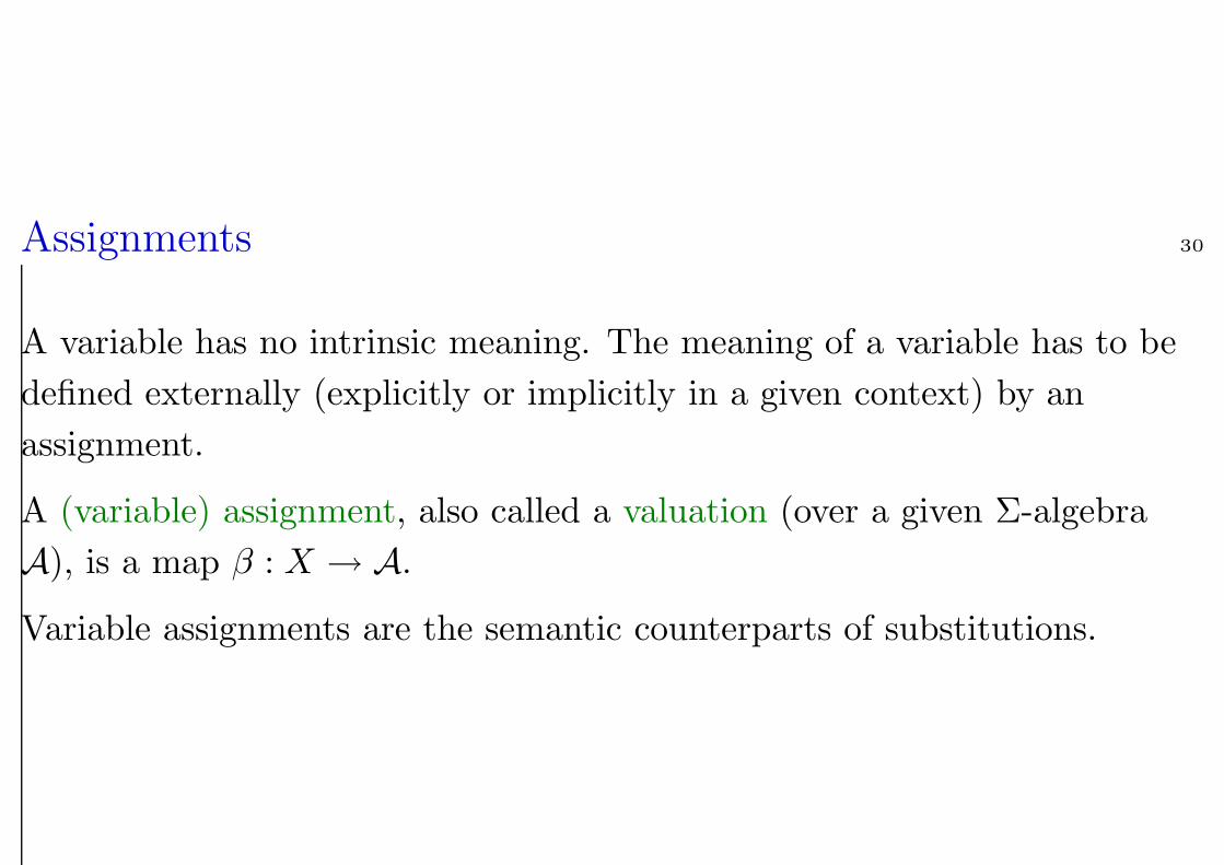
Assignments 30
A variable has no intrinsic meaning. The meaning of a variable has to be
defined externally (explicitly or implicitly in a given context) by an
assignment.
A (variable) assignment, also called a valuation (over a given Σ-algebra
A), is a map β : X → A.
Variable assignments are the semantic counterparts of substitutions.
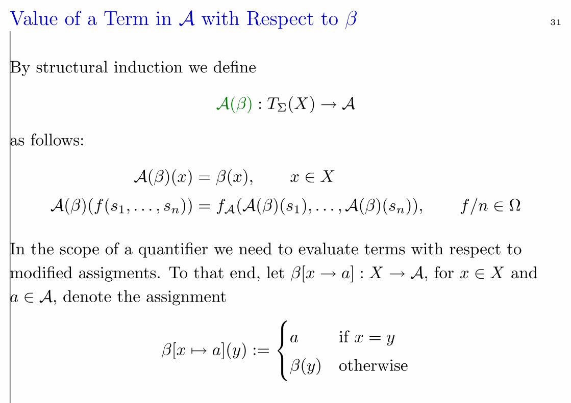
Value of a Term in A with Respect to β 31
By structural induction we define
A(β) : TΣ(X)→ A
as follows:
A(β)(x) = β(x), x ∈ X
A(β)(f(s1, . . . , sn)) = fA(A(β)(s1), . . . ,A(β)(sn)), f/n ∈ Ω
In the scope of a quantifier we need to evaluate terms with respect to
modified assigments. To that end, let β[x→ a] : X → A, for x ∈ X and
a ∈ A, denote the assignment
β[x 7→ a](y) :=
a if x = y
β(y) otherwise
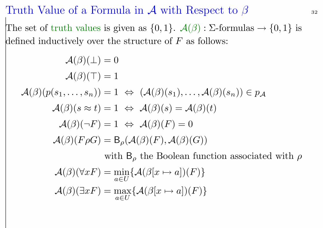
Truth Value of a Formula in A with Respect to β 32
The set of truth values is given as 0, 1. A(β) : Σ-formulas→ 0, 1 is
defined inductively over the structure of F as follows:
A(β)(⊥) = 0
A(β)(>) = 1
A(β)(p(s1, . . . , sn)) = 1 ⇔ (A(β)(s1), . . . ,A(β)(sn)) ∈ pA
A(β)(s ≈ t) = 1 ⇔ A(β)(s) = A(β)(t)
A(β)(¬F ) = 1 ⇔ A(β)(F ) = 0
A(β)(FρG) = Bρ(A(β)(F ),A(β)(G))
with Bρ the Boolean function associated with ρ
A(β)(∀xF ) = mina∈UA(β[x 7→ a])(F )
A(β)(∃xF ) = maxa∈UA(β[x 7→ a])(F )
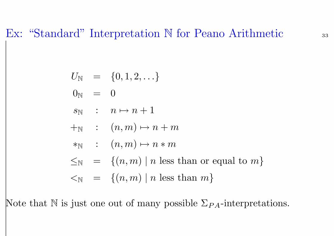
Ex: “Standard” Interpretation N for Peano Arithmetic 33
UN = 0, 1, 2, . . .
0N = 0
sN : n 7→ n + 1
+N : (n,m) 7→ n + m
∗N : (n,m) 7→ n ∗m
≤N = (n,m) | n less than or equal to m
<N = (n,m) | n less than m
Note that N is just one out of many possible ΣPA-interpretations.
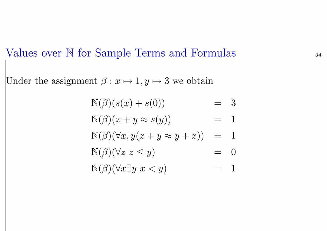
Values over N for Sample Terms and Formulas 34
Under the assignment β : x 7→ 1, y 7→ 3 we obtain
N(β)(s(x) + s(0)) = 3
N(β)(x + y ≈ s(y)) = 1
N(β)(∀x, y(x + y ≈ y + x)) = 1
N(β)(∀z z ≤ y) = 0
N(β)(∀x∃y x < y) = 1
1.3 Models, Validity, and Satisfiability 35
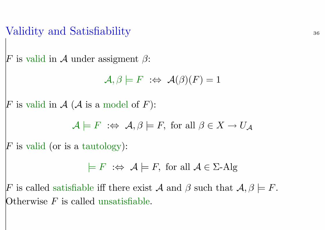
Validity and Satisfiability 36
F is valid in A under assigment β:
A, β |= F :⇔ A(β)(F ) = 1
F is valid in A (A is a model of F ):
A |= F :⇔ A, β |= F, for all β ∈ X → UA
F is valid (or is a tautology):
|= F :⇔ A |= F, for all A ∈ Σ-Alg
F is called satisfiable iff there exist A and β such that A, β |= F .
Otherwise F is called unsatisfiable.
Substitution Lemma 37
The following theorems, to be proved by structural induction, hold for all
Σ-algebras A, assignments β, and substitutions σ.
Theorem 1.3 For any Σ-term t
A(β)(tσ) = A(β σ)(t),
where β σ : X → A is the assignment β σ(x) = A(β)(xσ).
Theorem 1.4 For any Σ-formula F , A(β)(Fσ) = A(β σ)(F ).
Corollary 1.5 A, β |= Fσ ⇔ A, β σ |= F
These theorems basically express that the syntactic concept of substitution
corresponds to the semantic concept of an assignment.
Entailment and Equivalence 38
F entails (implies) G (or G is entailed by F ), written F |= G
:⇔ for all A ∈ Σ-Alg and β ∈ X → UA, whenever A, β |= F then
A, β |= G.
F and G are called equivalent
:⇔ for all A ∈ Σ-Alg und β ∈ X → UA we have A, β |= F ⇔ A, β |= G.
Proposition 1.1 F entails G iff (F → G) is valid
Proposition 1.2 F and G are equivalent iff (F ↔ G) is valid.
Extension to sets of formulas N in the “natural way”, e.g., N |= F
:⇔ for all A ∈ Σ-Alg and β ∈ X → UA:
if A, β |= G, for all G ∈ N , then A, β |= F .
Validity vs. Unsatisfiability 39
Validity and unsatisfiability are just two sides of the same medal as
explained by the following proposition.
Proposition 1.3
F valid ⇔ ¬F unsatisfiable
Hence in order to design a theorem prover (validity checker) it is sufficient
to design a checker for unsatisfiability.
Q: In a similar way, entailment N |= F can be reduced to unsatisfiability.
How?
Theory of a Structure 40
Let A ∈ Σ-Alg. The (first-order) theory of A is defined as
Th(A) =df G ∈ FΣ(X) | A |= G
Problem of axiomatizability:
For which structures A can one axiomatize Th(A), that is, can one write
down a formula F (or a recursively enumerable set F of formulas) such
that
Th(A) = G | F |= G?
Analoguously for sets of structures.
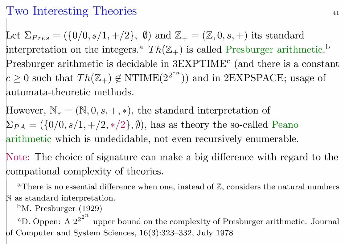
Two Interesting Theories 41
Let ΣPres = (0/0, s/1,+/2, ∅) and Z+ = (Z, 0, s,+) its standard
interpretation on the integers.a Th(Z+) is called Presburger arithmetic.b
Presburger arithmetic is decidable in 3EXPTIMEc (and there is a constant
c ≥ 0 such that Th(Z+) 6∈ NTIME(22cn
)) and in 2EXPSPACE; usage of
automata-theoretic methods.
However, N∗ = (N, 0, s,+, ∗), the standard interpretation of
ΣPA = (0/0, s/1,+/2, ∗/2, ∅), has as theory the so-called Peano
arithmetic which is undedidable, not even recursively enumerable.
Note: The choice of signature can make a big difference with regard to the
compational complexity of theories.aThere is no essential difference when one, instead of Z, considers the natural numbers
N as standard interpretation.bM. Presburger (1929)
cD. Oppen: A 222n
upper bound on the complexity of Presburger arithmetic. Journal
of Computer and System Sciences, 16(3):323–332, July 1978
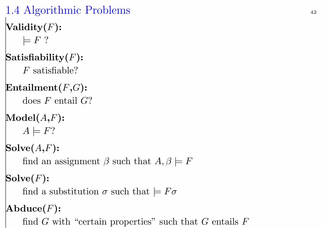
1.4 Algorithmic Problems 42
Validity(F ):
|= F ?
Satisfiability(F ):
F satisfiable?
Entailment(F ,G):
does F entail G?
Model(A,F ):
A |= F?
Solve(A,F ):
find an assignment β such that A, β |= F
Solve(F ):
find a substitution σ such that |= Fσ
Abduce(F ):
find G with “certain properties” such that G entails F
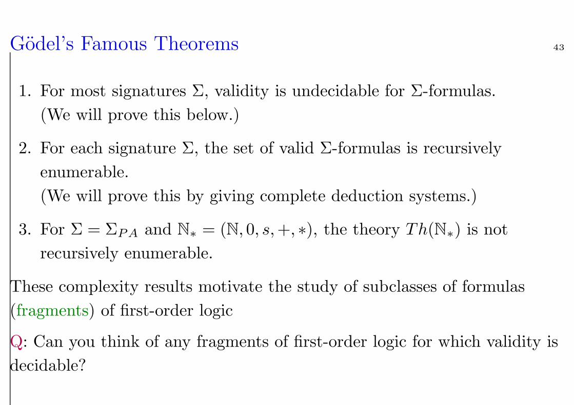
Godel’s Famous Theorems 43
1. For most signatures Σ, validity is undecidable for Σ-formulas.
(We will prove this below.)
2. For each signature Σ, the set of valid Σ-formulas is recursively
enumerable.
(We will prove this by giving complete deduction systems.)
3. For Σ = ΣPA and N∗ = (N, 0, s,+, ∗), the theory Th(N∗) is not
recursively enumerable.
These complexity results motivate the study of subclasses of formulas
(fragments) of first-order logic
Q: Can you think of any fragments of first-order logic for which validity is
decidable?
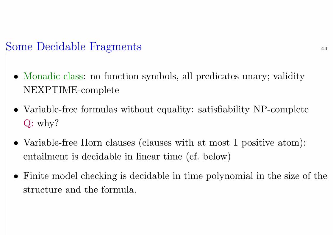
Some Decidable Fragments 44
• Monadic class: no function symbols, all predicates unary; validity
NEXPTIME-complete
• Variable-free formulas without equality: satisfiability NP-complete
Q: why?
• Variable-free Horn clauses (clauses with at most 1 positive atom):
entailment is decidable in linear time (cf. below)
• Finite model checking is decidable in time polynomial in the size of the
structure and the formula.
1.5 Normal Forms, Skolemization, Herbrand Models 45
Study of normal forms motivated by
• reduction of logical concepts,
• efficient data structures for theorem proving.
The main problem in first-order logic is the treatment of quantifiers. The
subsequent normal form transformations are intended to eliminate many of
them.
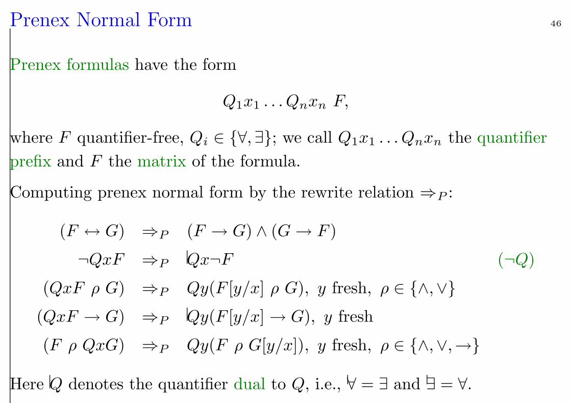
Prenex Normal Form 46
Prenex formulas have the form
Q1x1 . . . Qnxn F,
where F quantifier-free, Qi ∈ ∀,∃; we call Q1x1 . . . Qnxn the quantifier
prefix and F the matrix of the formula.
Computing prenex normal form by the rewrite relation ⇒P :
(F ↔ G) ⇒P (F → G) ∧ (G→ F )
¬QxF ⇒P Qx¬F (¬Q)
(QxF ρ G) ⇒P Qy(F [y/x] ρ G), y fresh, ρ ∈ ∧,∨
(QxF → G) ⇒P Qy(F [y/x]→ G), y fresh
(F ρ QxG) ⇒P Qy(F ρ G[y/x]), y fresh, ρ ∈ ∧,∨,→
Here Q denotes the quantifier dual to Q, i.e., ∀ = ∃ and ∃ = ∀.
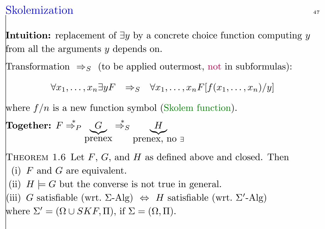
Skolemization 47
Intuition: replacement of ∃y by a concrete choice function computing y
from all the arguments y depends on.
Transformation ⇒S (to be applied outermost, not in subformulas):
∀x1, . . . , xn∃yF ⇒S ∀x1, . . . , xnF [f(x1, . . . , xn)/y]
where f/n is a new function symbol (Skolem function).
Together: F∗⇒P G
︸︷︷︸
prenex
∗⇒S H
︸︷︷︸
prenex, no ∃
Theorem 1.6 Let F , G, and H as defined above and closed. Then
(i) F and G are equivalent.
(ii) H |= G but the converse is not true in general.
(iii) G satisfiable (wrt. Σ-Alg) ⇔ H satisfiable (wrt. Σ′-Alg)
where Σ′ = (Ω ∪ SKF,Π), if Σ = (Ω,Π).
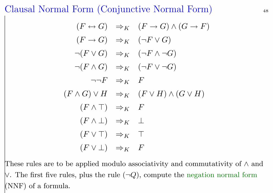
Clausal Normal Form (Conjunctive Normal Form) 48
(F ↔ G) ⇒K (F → G) ∧ (G→ F )
(F → G) ⇒K (¬F ∨G)
¬(F ∨G) ⇒K (¬F ∧ ¬G)
¬(F ∧G) ⇒K (¬F ∨ ¬G)
¬¬F ⇒K F
(F ∧G) ∨H ⇒K (F ∨H) ∧ (G ∨H)
(F ∧ >) ⇒K F
(F ∧ ⊥) ⇒K ⊥
(F ∨ >) ⇒K >
(F ∨ ⊥) ⇒K F
These rules are to be applied modulo associativity and commutativity of ∧ and
∨. The first five rules, plus the rule (¬Q), compute the negation normal form
(NNF) of a formula.
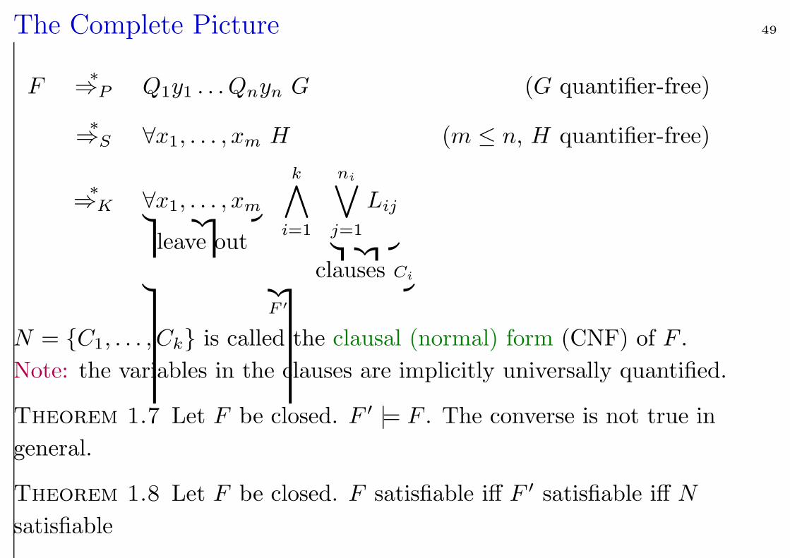
The Complete Picture 49
F∗⇒P Q1y1 . . . Qnyn G (G quantifier-free)
∗⇒S ∀x1, . . . , xm H (m ≤ n, H quantifier-free)
∗⇒K ∀x1, . . . , xm
︸ ︷︷ ︸
leave out
k∧
i=1
ni∨
j=1
Lij
︸ ︷︷ ︸
clauses Ci︸ ︷︷ ︸
F ′
N = C1, . . . , Ck is called the clausal (normal) form (CNF) of F .
Note: the variables in the clauses are implicitly universally quantified.
Theorem 1.7 Let F be closed. F ′ |= F . The converse is not true in
general.
Theorem 1.8 Let F be closed. F satisfiable iff F ′ satisfiable iff N
satisfiable
Optimization 50
Here is lots of room for optimization since we only can preserve
satisfiability anyway:
• size of the CNF exponential when done naively;
• want to preserve the original formula structure;
• want small arity of Skolem functions (cf. Info IV and tutorials)!
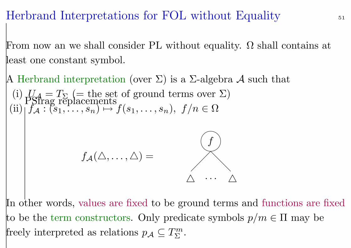
Herbrand Interpretations for FOL without Equality 51
From now an we shall consider PL without equality. Ω shall contains at
least one constant symbol.
A Herbrand interpretation (over Σ) is a Σ-algebra A such that
(i) UA = TΣ (= the set of ground terms over Σ)
(ii) fA : (s1, . . . , sn) 7→ f(s1, . . . , sn), f/n ∈ ΩPSfrag replacements
f
fA(4, . . . ,4) =
4 . . . 4
In other words, values are fixed to be ground terms and functions are fixed
to be the term constructors. Only predicate symbols p/m ∈ Π may be
freely interpreted as relations pA ⊆ T mΣ .
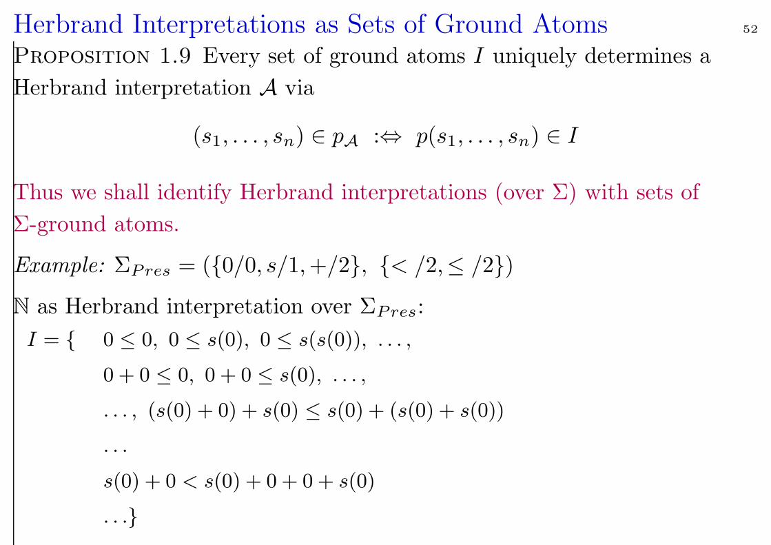
Herbrand Interpretations as Sets of Ground Atoms 52
Proposition 1.9 Every set of ground atoms I uniquely determines a
Herbrand interpretation A via
(s1, . . . , sn) ∈ pA :⇔ p(s1, . . . , sn) ∈ I
Thus we shall identify Herbrand interpretations (over Σ) with sets of
Σ-ground atoms.
Example: ΣPres = (0/0, s/1,+/2, < /2,≤ /2)
N as Herbrand interpretation over ΣPres:
I = 0 ≤ 0, 0 ≤ s(0), 0 ≤ s(s(0)), . . . ,
0 + 0 ≤ 0, 0 + 0 ≤ s(0), . . . ,
. . . , (s(0) + 0) + s(0) ≤ s(0) + (s(0) + s(0))
. . .
s(0) + 0 < s(0) + 0 + 0 + s(0)
. . .

Existence of Herbrand Models 53
A Herbrand interpretation I is called a Herbrand model of F ,
if I |= F .
Theorem 1.10 (Herbrand) Let N be a set of Σ clauses.
N satisfiable ⇔ N has a Herbrand model (over Σ)
⇔ GΣ(N) has a Herbrand model (over Σ)
where
GΣ(N) = Cσ ground clause | C ∈ N, σ : X → TΣ
the set of ground instances of N .
[Proof to be given below in the context of the completeness proof for
resolution.]
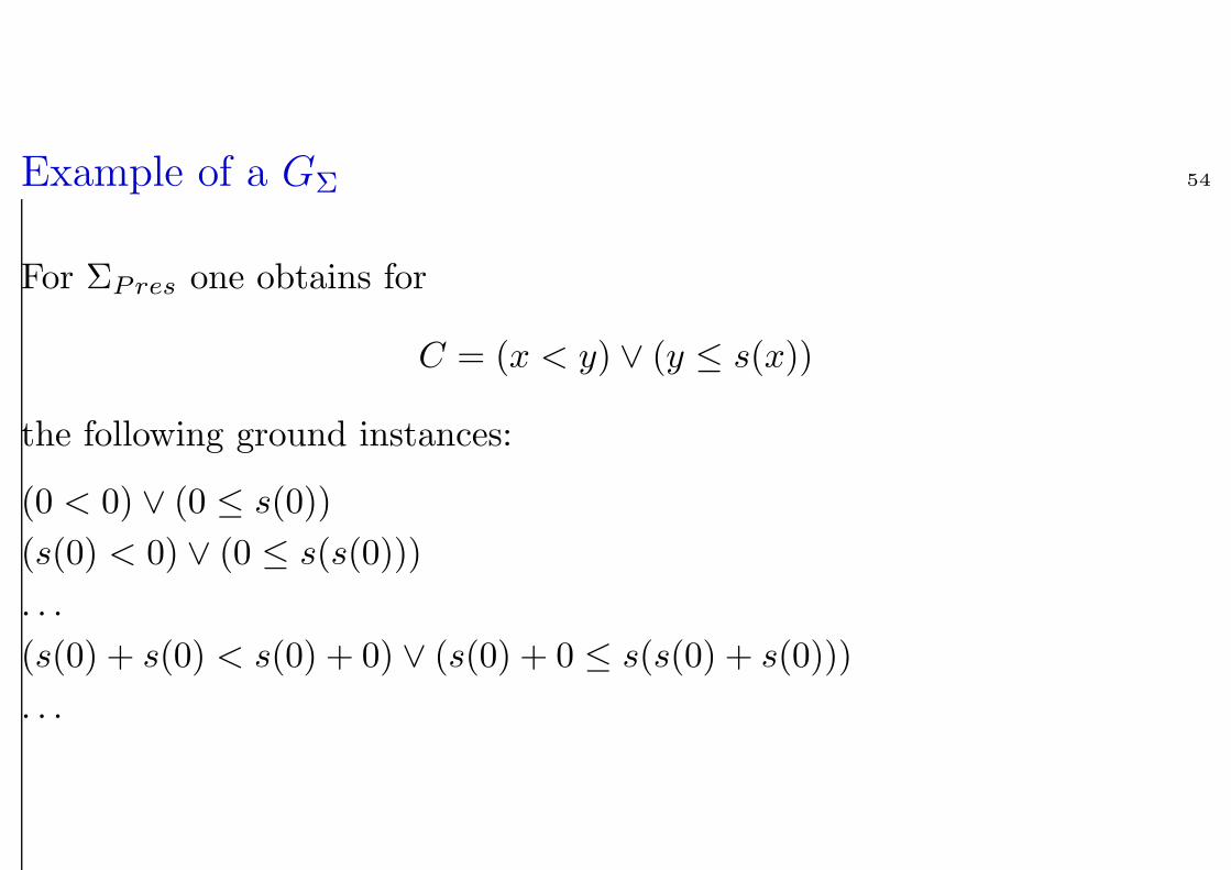
Example of a GΣ 54
For ΣPres one obtains for
C = (x < y) ∨ (y ≤ s(x))
the following ground instances:
(0 < 0) ∨ (0 ≤ s(0))
(s(0) < 0) ∨ (0 ≤ s(s(0)))
. . .
(s(0) + s(0) < s(0) + 0) ∨ (s(0) + 0 ≤ s(s(0) + s(0)))
. . .
1.6 Inference Systems, Proofs 55
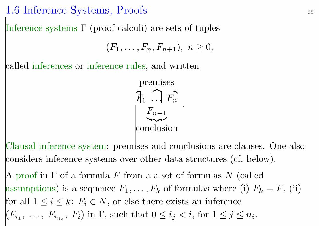
Inference systems Γ (proof calculi) are sets of tuples
(F1, . . . , Fn, Fn+1), n ≥ 0,
called inferences or inference rules, and written
premises︷ ︸︸ ︷
F1 . . . Fn
Fn+1︸ ︷︷ ︸
conclusion
.
Clausal inference system: premises and conclusions are clauses. One also
considers inference systems over other data structures (cf. below).
A proof in Γ of a formula F from a a set of formulas N (called
assumptions) is a sequence F1, . . . , Fk of formulas where (i) Fk = F , (ii)
for all 1 ≤ i ≤ k: Fi ∈ N , or else there exists an inference
(Fi1 , . . . , Fini, Fi) in Γ, such that 0 ≤ ij < i, for 1 ≤ j ≤ ni.
Soundness, Completeness 56
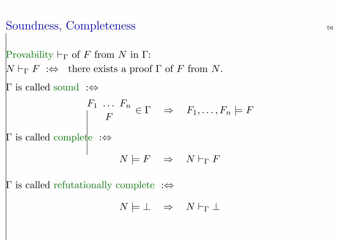
Provability `Γ of F from N in Γ:
N `Γ F :⇔ there exists a proof Γ of F from N .
Γ is called sound :⇔
F1 . . . Fn
F∈ Γ ⇒ F1, . . . , Fn |= F
Γ is called complete :⇔
N |= F ⇒ N `Γ F
Γ is called refutationally complete :⇔
N |= ⊥ ⇒ N `Γ ⊥
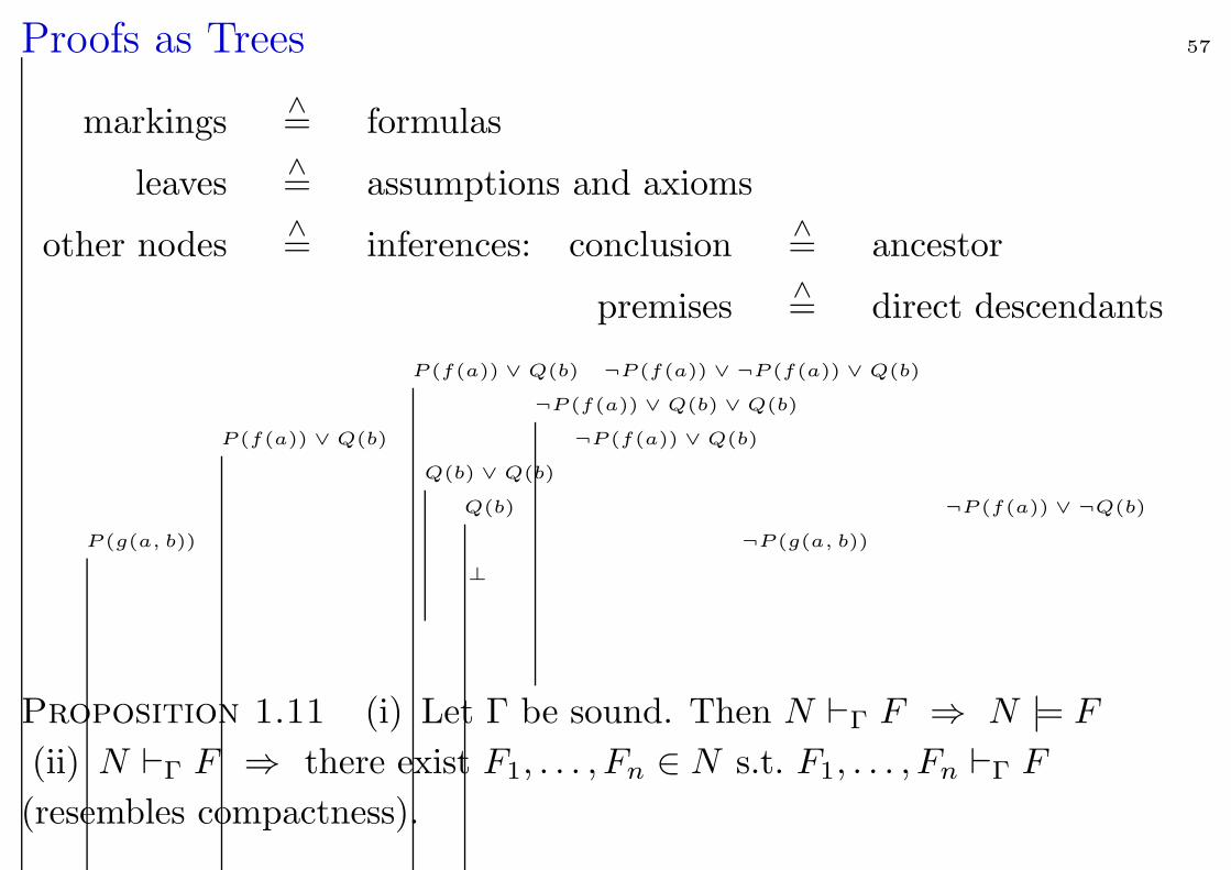
Proofs as Trees 57
markings∧= formulas
leaves∧= assumptions and axioms
other nodes∧= inferences: conclusion
∧= ancestor
premises∧= direct descendants
P (g(a, b))
P (f(a)) ∨ Q(b)
P (f(a)) ∨ Q(b) ¬P (f(a)) ∨ ¬P (f(a)) ∨ Q(b)
¬P (f(a)) ∨ Q(b) ∨ Q(b)
¬P (f(a)) ∨ Q(b)
Q(b) ∨ Q(b)
Q(b) ¬P (f(a)) ∨ ¬Q(b)
¬P (g(a, b))
⊥
Proposition 1.11 (i) Let Γ be sound. Then N `Γ F ⇒ N |= F
(ii) N `Γ F ⇒ there exist F1, . . . , Fn ∈ N s.t. F1, . . . , Fn `Γ F
(resembles compactness).
1.7 Propositional Resolution 58
We observe that propositional clauses and ground clauses are the same
concept.
In this section we only deal with ground clauses.
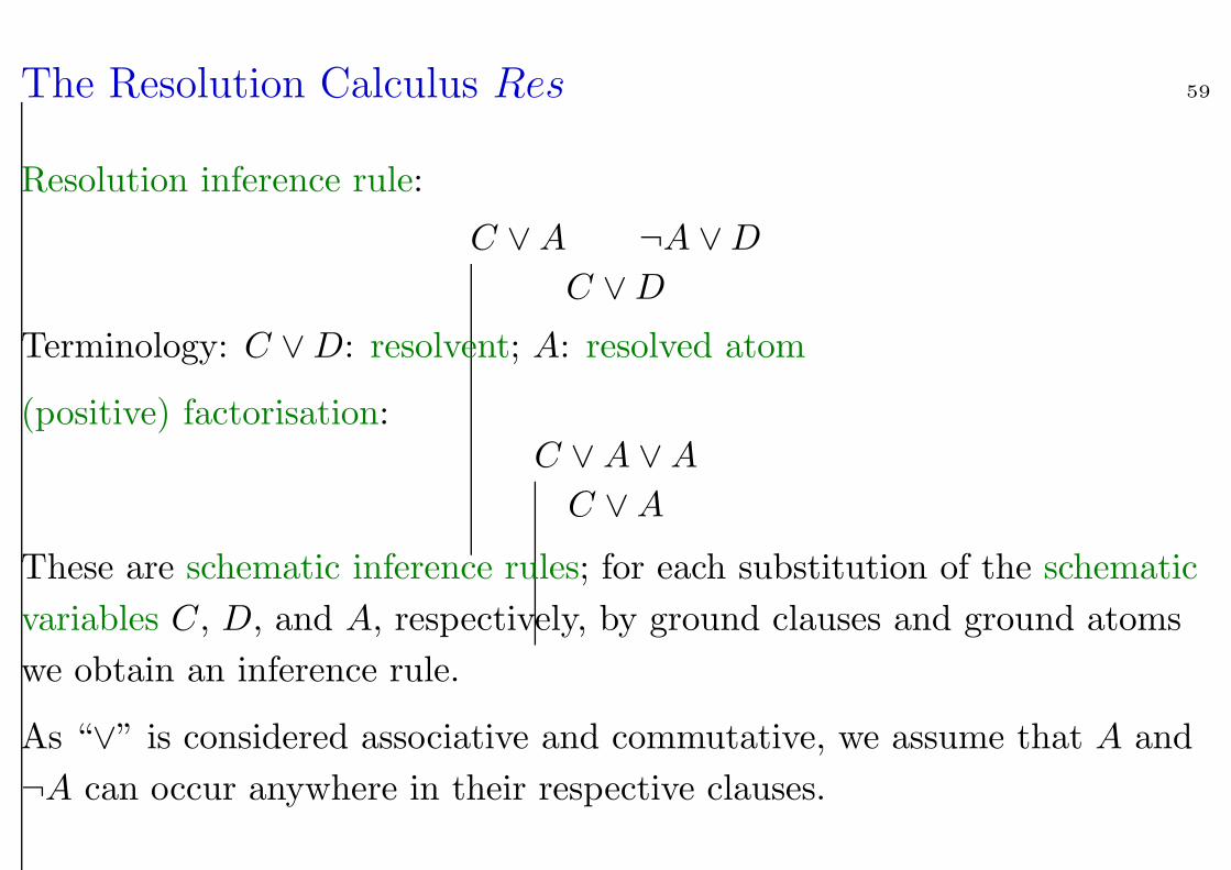
The Resolution Calculus Res 59
Resolution inference rule:
C ∨A ¬A ∨D
C ∨D
Terminology: C ∨D: resolvent; A: resolved atom
(positive) factorisation:C ∨A ∨A
C ∨A
These are schematic inference rules; for each substitution of the schematic
variables C, D, and A, respectively, by ground clauses and ground atoms
we obtain an inference rule.
As “∨” is considered associative and commutative, we assume that A and
¬A can occur anywhere in their respective clauses.
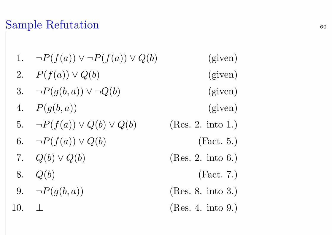
Sample Refutation 60
1. ¬P (f(a)) ∨ ¬P (f(a)) ∨Q(b) (given)
2. P (f(a)) ∨Q(b) (given)
3. ¬P (g(b, a)) ∨ ¬Q(b) (given)
4. P (g(b, a)) (given)
5. ¬P (f(a)) ∨Q(b) ∨Q(b) (Res. 2. into 1.)
6. ¬P (f(a)) ∨Q(b) (Fact. 5.)
7. Q(b) ∨Q(b) (Res. 2. into 6.)
8. Q(b) (Fact. 7.)
9. ¬P (g(b, a)) (Res. 8. into 3.)
10. ⊥ (Res. 4. into 9.)
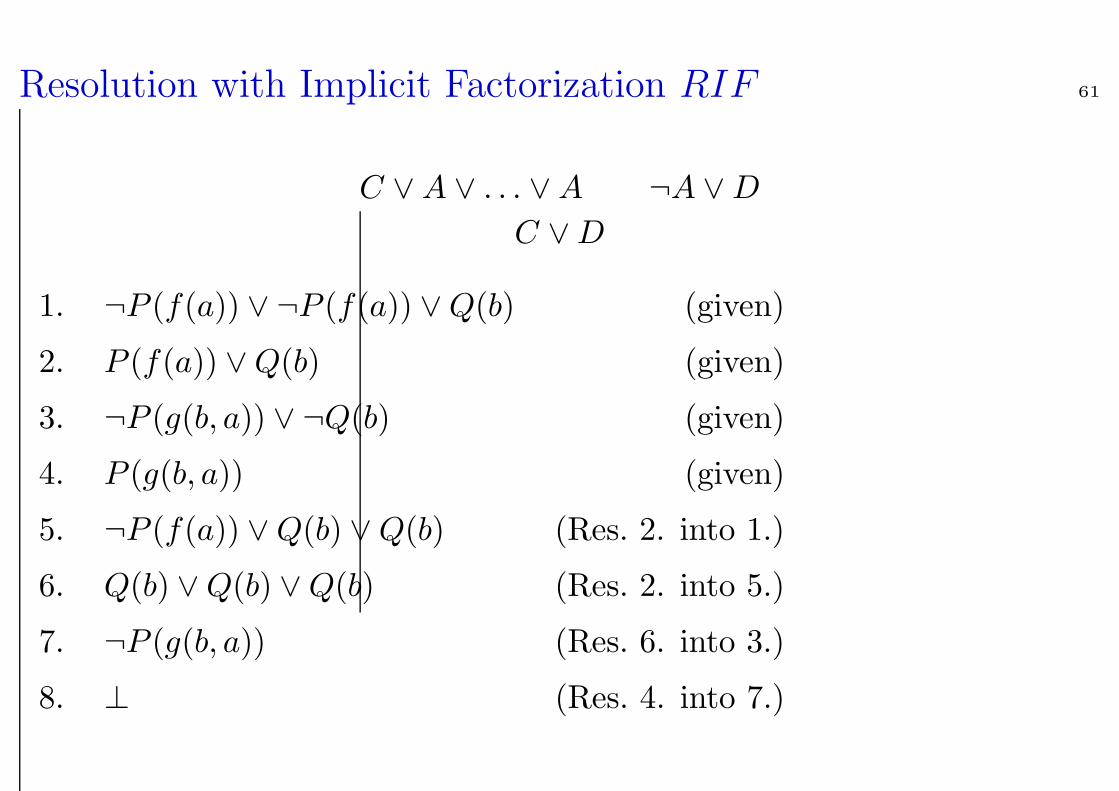
Resolution with Implicit Factorization RIF 61
C ∨A ∨ . . . ∨A ¬A ∨D
C ∨D
1. ¬P (f(a)) ∨ ¬P (f(a)) ∨Q(b) (given)
2. P (f(a)) ∨Q(b) (given)
3. ¬P (g(b, a)) ∨ ¬Q(b) (given)
4. P (g(b, a)) (given)
5. ¬P (f(a)) ∨Q(b) ∨Q(b) (Res. 2. into 1.)
6. Q(b) ∨Q(b) ∨Q(b) (Res. 2. into 5.)
7. ¬P (g(b, a)) (Res. 6. into 3.)
8. ⊥ (Res. 4. into 7.)
Another Example 62
Soundness of Resolution 63
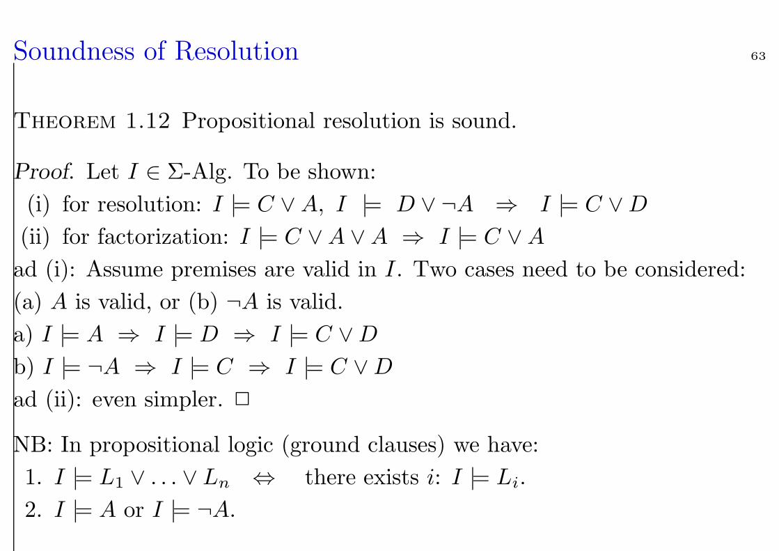
Theorem 1.12 Propositional resolution is sound.
Proof. Let I ∈ Σ-Alg. To be shown:
(i) for resolution: I |= C ∨A, I |= D ∨ ¬A ⇒ I |= C ∨D
(ii) for factorization: I |= C ∨A ∨A ⇒ I |= C ∨A
ad (i): Assume premises are valid in I. Two cases need to be considered:
(a) A is valid, or (b) ¬A is valid.
a) I |= A ⇒ I |= D ⇒ I |= C ∨D
b) I |= ¬A ⇒ I |= C ⇒ I |= C ∨D
ad (ii): even simpler. 2
NB: In propositional logic (ground clauses) we have:
1. I |= L1 ∨ . . . ∨ Ln ⇔ there exists i: I |= Li.
2. I |= A or I |= ¬A.
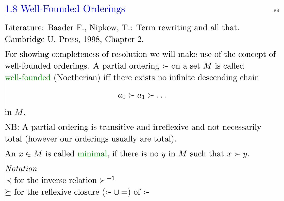
1.8 Well-Founded Orderings 64
Literature: Baader F., Nipkow, T.: Term rewriting and all that.
Cambridge U. Press, 1998, Chapter 2.
For showing completeness of resolution we will make use of the concept of
well-founded orderings. A partial ordering on a set M is called
well-founded (Noetherian) iff there exists no infinite descending chain
a0 a1 . . .
in M .
NB: A partial ordering is transitive and irreflexive and not necessarily
total (however our orderings usually are total).
An x ∈M is called minimal, if there is no y in M such that x y.
Notation
≺ for the inverse relation −1
for the reflexive closure ( ∪=) of
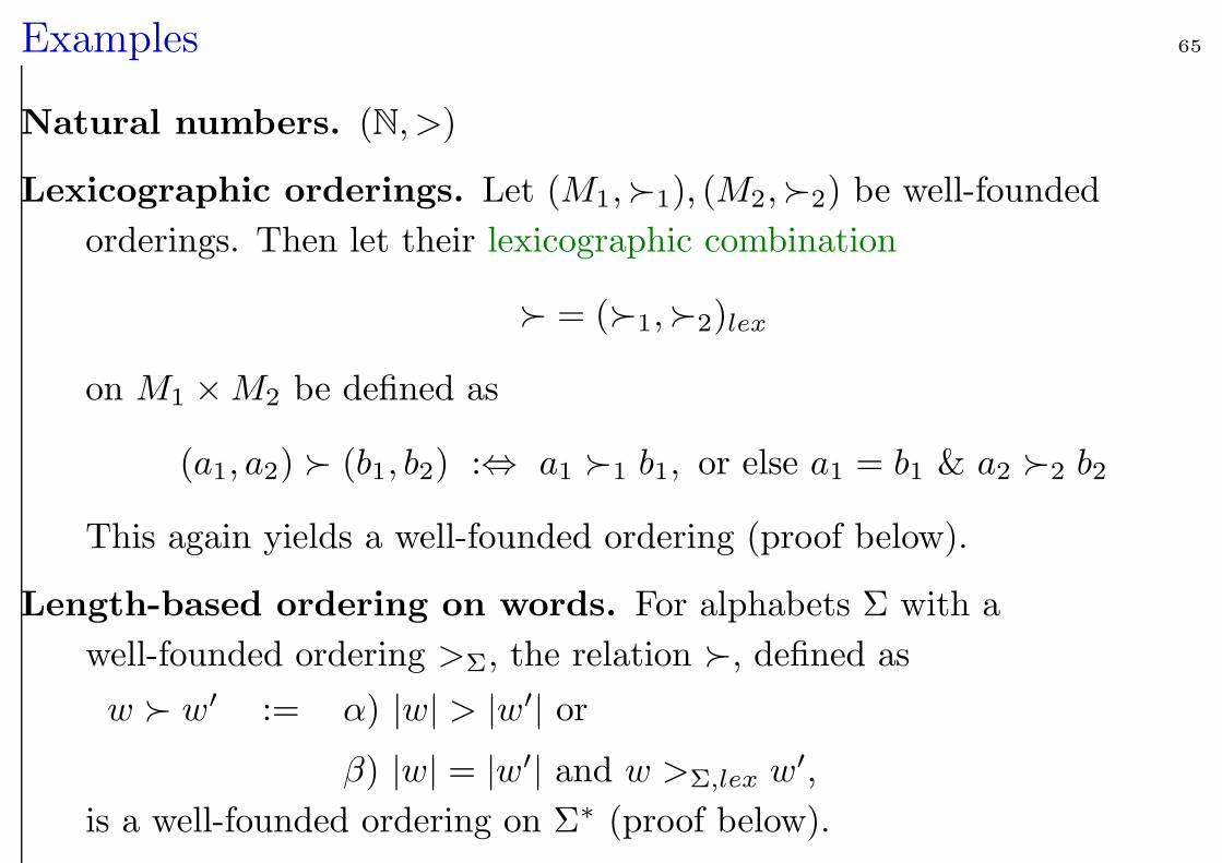
Examples 65
Natural numbers. (N, >)
Lexicographic orderings. Let (M1,1), (M2,2) be well-founded
orderings. Then let their lexicographic combination
= (1,2)lex
on M1 ×M2 be defined as
(a1, a2) (b1, b2) :⇔ a1 1 b1, or else a1 = b1 & a2 2 b2
This again yields a well-founded ordering (proof below).
Length-based ordering on words. For alphabets Σ with a
well-founded ordering >Σ, the relation , defined as
w w′ := α) |w| > |w′| or
β) |w| = |w′| and w >Σ,lex w′,
is a well-founded ordering on Σ∗ (proof below).
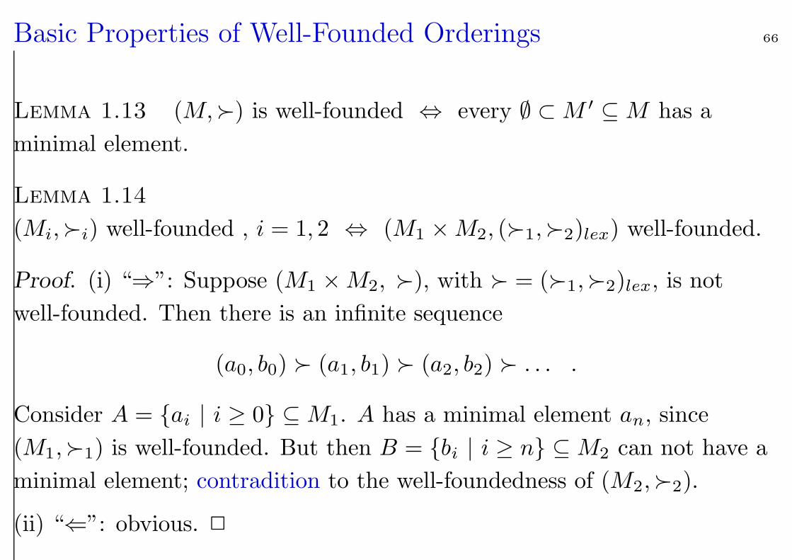
Basic Properties of Well-Founded Orderings 66
Lemma 1.13 (M,) is well-founded ⇔ every ∅ ⊂M ′ ⊆M has a
minimal element.
Lemma 1.14
(Mi,i) well-founded , i = 1, 2 ⇔ (M1 ×M2, (1,2)lex) well-founded.
Proof. (i) “⇒”: Suppose (M1 ×M2, ), with = (1,2)lex, is not
well-founded. Then there is an infinite sequence
(a0, b0) (a1, b1) (a2, b2) . . . .
Consider A = ai | i ≥ 0 ⊆M1. A has a minimal element an, since
(M1,1) is well-founded. But then B = bi | i ≥ n ⊆M2 can not have a
minimal element; contradition to the well-foundedness of (M2,2).
(ii) “⇐”: obvious. 2
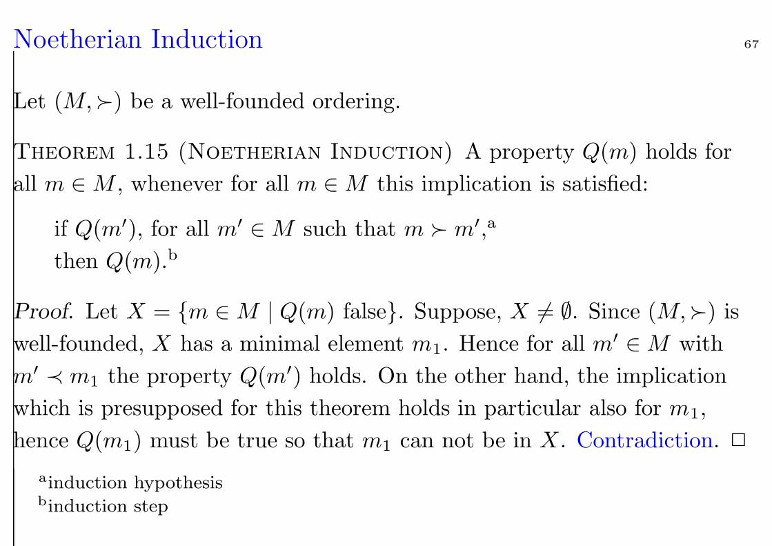
Noetherian Induction 67
Let (M,) be a well-founded ordering.
Theorem 1.15 (Noetherian Induction) A property Q(m) holds for
all m ∈M , whenever for all m ∈M this implication is satisfied:
if Q(m′), for all m′ ∈M such that m m′,a
then Q(m).b
Proof. Let X = m ∈M | Q(m) false. Suppose, X 6= ∅. Since (M,) is
well-founded, X has a minimal element m1. Hence for all m′ ∈M with
m′ ≺ m1 the property Q(m′) holds. On the other hand, the implication
which is presupposed for this theorem holds in particular also for m1,
hence Q(m1) must be true so that m1 can not be in X. Contradiction. 2
ainduction hypothesisbinduction step
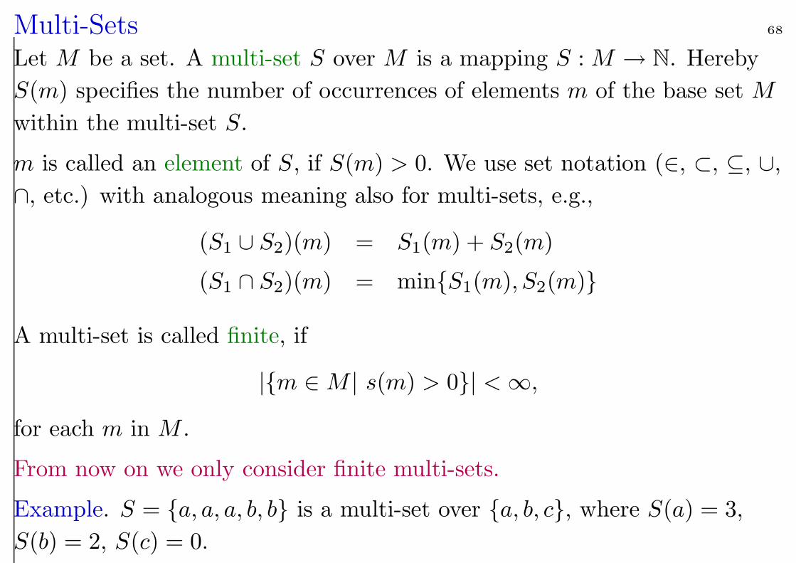
Multi-Sets 68
Let M be a set. A multi-set S over M is a mapping S : M → N. Hereby
S(m) specifies the number of occurrences of elements m of the base set M
within the multi-set S.
m is called an element of S, if S(m) > 0. We use set notation (∈, ⊂, ⊆, ∪,
∩, etc.) with analogous meaning also for multi-sets, e.g.,
(S1 ∪ S2)(m) = S1(m) + S2(m)
(S1 ∩ S2)(m) = minS1(m), S2(m)
A multi-set is called finite, if
|m ∈M | s(m) > 0| <∞,
for each m in M .
From now on we only consider finite multi-sets.
Example. S = a, a, a, b, b is a multi-set over a, b, c, where S(a) = 3,
S(b) = 2, S(c) = 0.
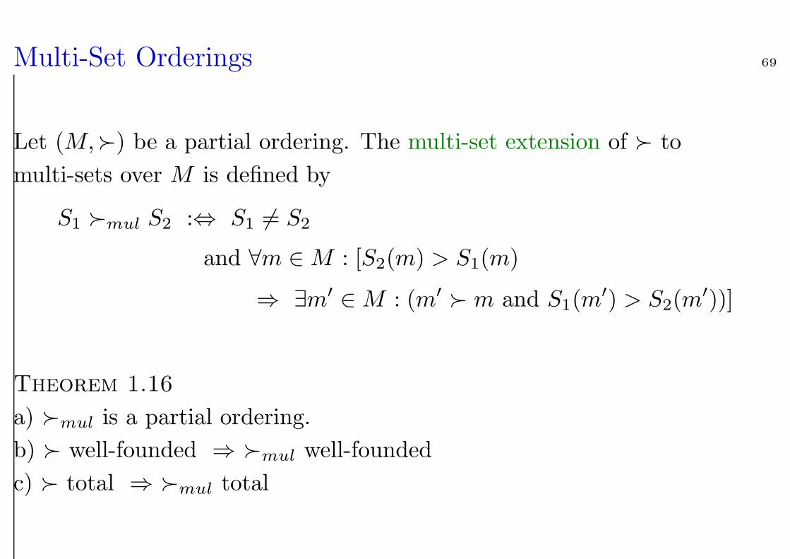
Multi-Set Orderings 69
Let (M,) be a partial ordering. The multi-set extension of to
multi-sets over M is defined by
S1 mul S2 :⇔ S1 6= S2
and ∀m ∈M : [S2(m) > S1(m)
⇒ ∃m′ ∈M : (m′ m and S1(m′) > S2(m
′))]
Theorem 1.16
a) mul is a partial ordering.
b) well-founded ⇒ mul well-founded
c) total ⇒ mul total
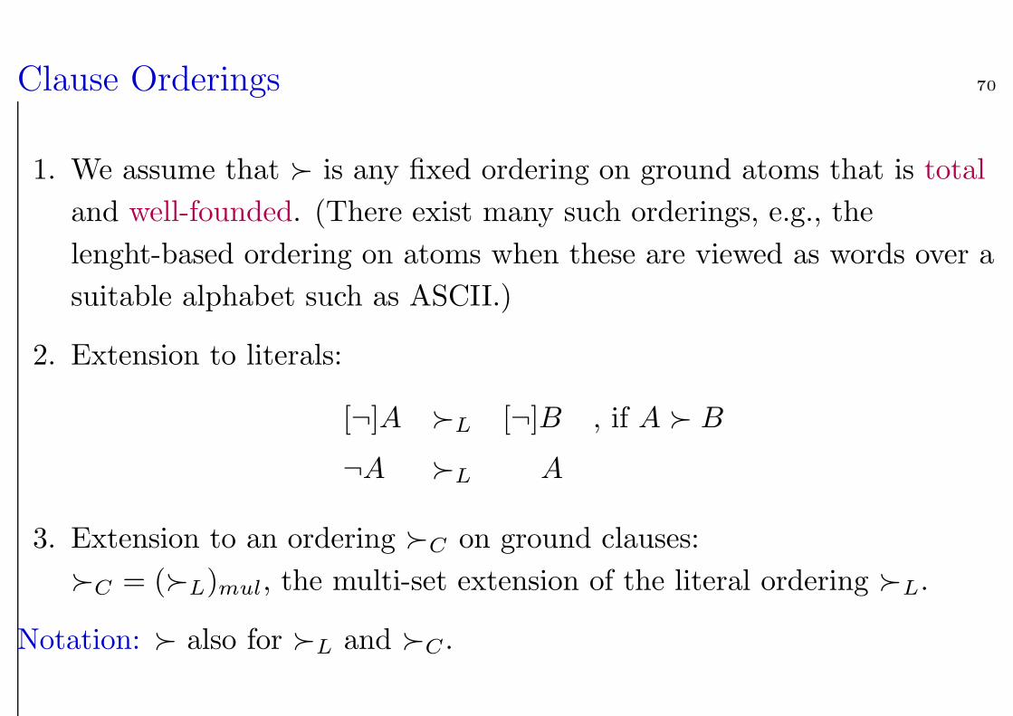
Clause Orderings 70
1. We assume that is any fixed ordering on ground atoms that is total
and well-founded. (There exist many such orderings, e.g., the
lenght-based ordering on atoms when these are viewed as words over a
suitable alphabet such as ASCII.)
2. Extension to literals:
[¬]A L [¬]B , if A B
¬A L A
3. Extension to an ordering C on ground clauses:
C = (L)mul, the multi-set extension of the literal ordering L.
Notation: also for L and C .
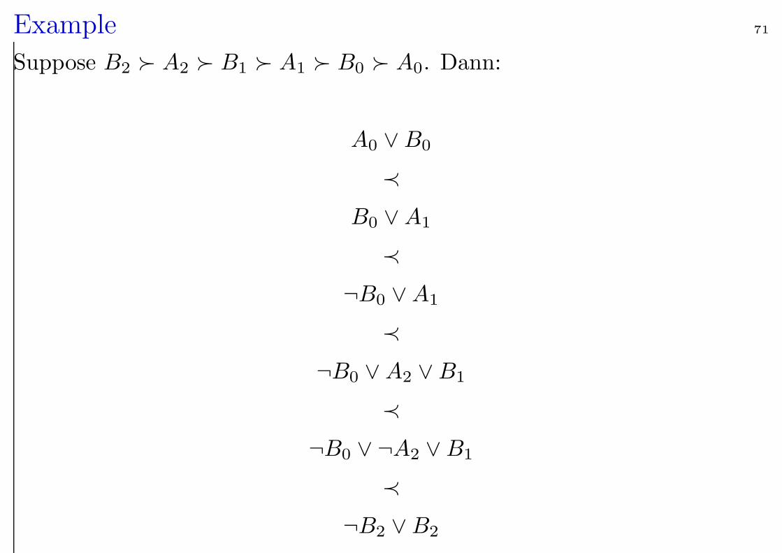
Example 71
Suppose B2 A2 B1 A1 B0 A0. Dann:
A0 ∨B0
≺
B0 ∨A1
≺
¬B0 ∨A1
≺
¬B0 ∨A2 ∨B1
≺
¬B0 ∨ ¬A2 ∨B1
≺
¬B2 ∨B2
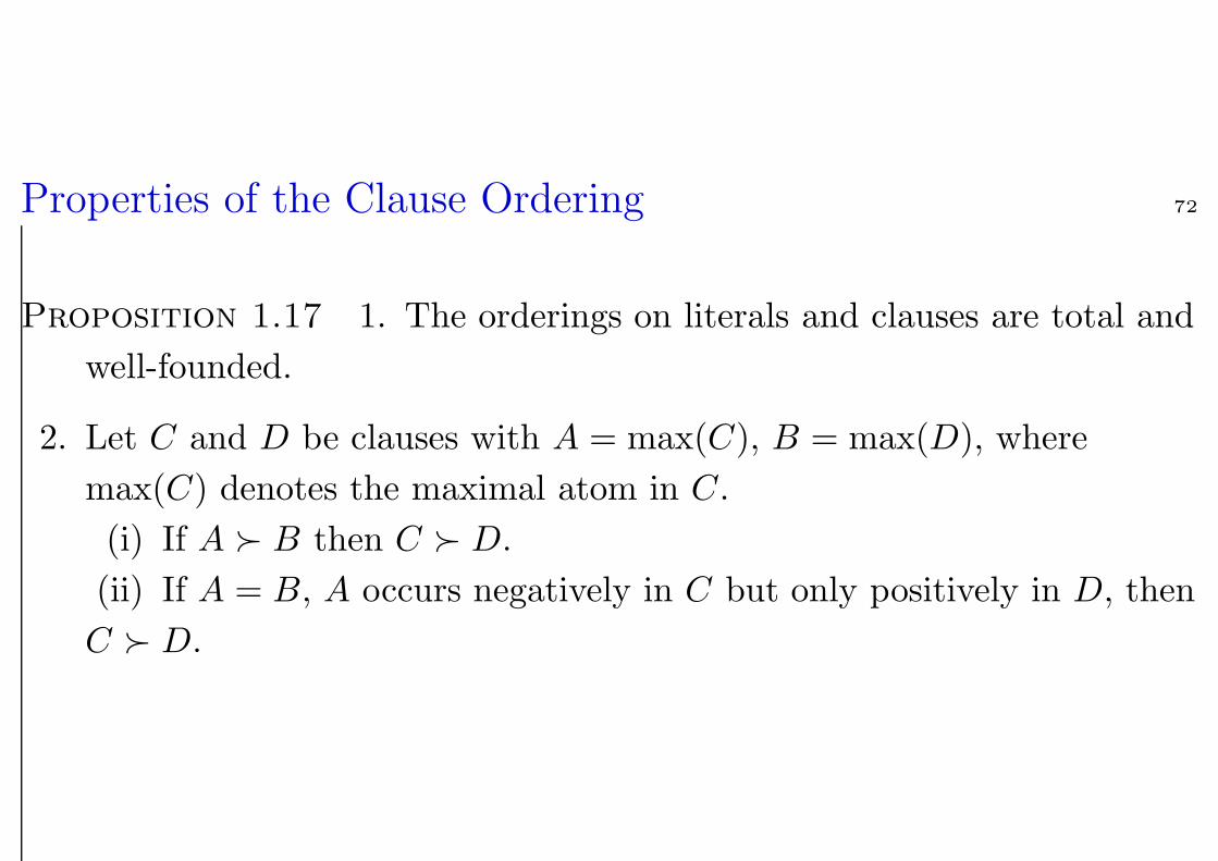
Properties of the Clause Ordering 72
Proposition 1.17 1. The orderings on literals and clauses are total and
well-founded.
2. Let C and D be clauses with A = max(C), B = max(D), where
max(C) denotes the maximal atom in C.
(i) If A B then C D.
(ii) If A = B, A occurs negatively in C but only positively in D, then
C D.
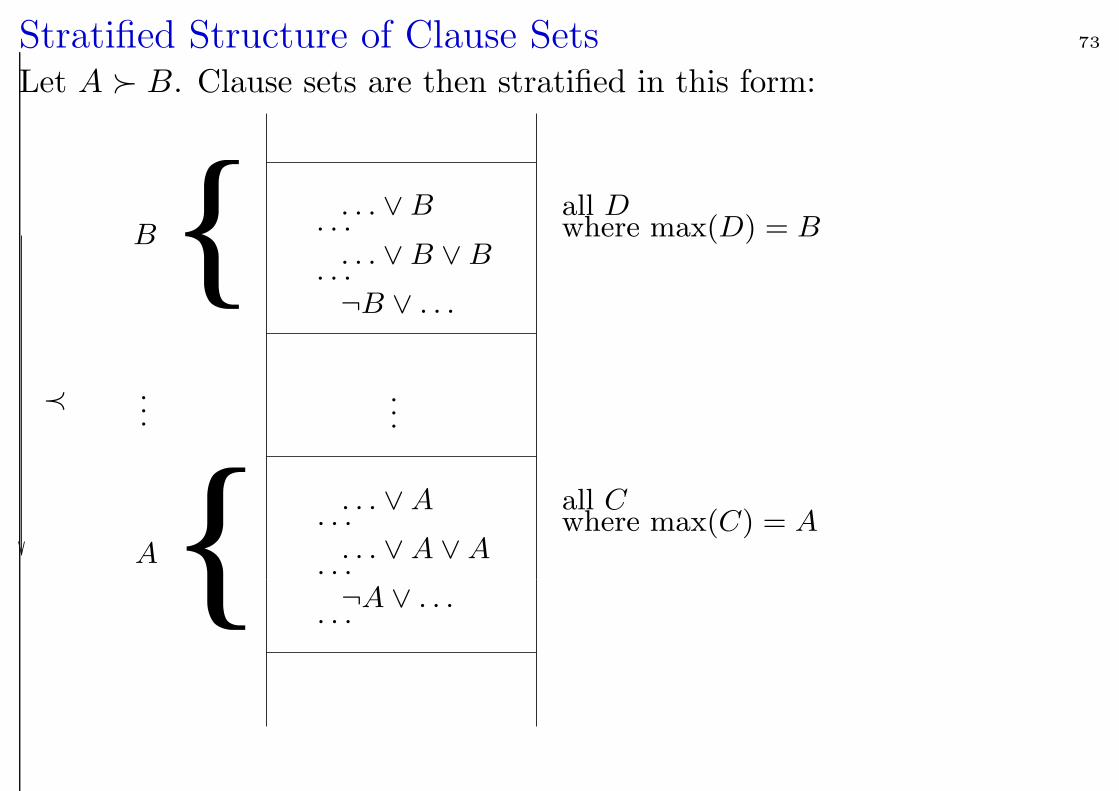
Stratified Structure of Clause Sets 73
Let A B. Clause sets are then stratified in this form:
PSfrag replacements
......
≺
A
B. . . ∨ B
. . .. . . ∨ B ∨ B
. . .¬B ∨ . . .
. . . ∨ A. . .
. . . ∨ A ∨ A. . .¬A ∨ . . .
. . .
all Dwhere max(D) = B
all Cwhere max(C) = A
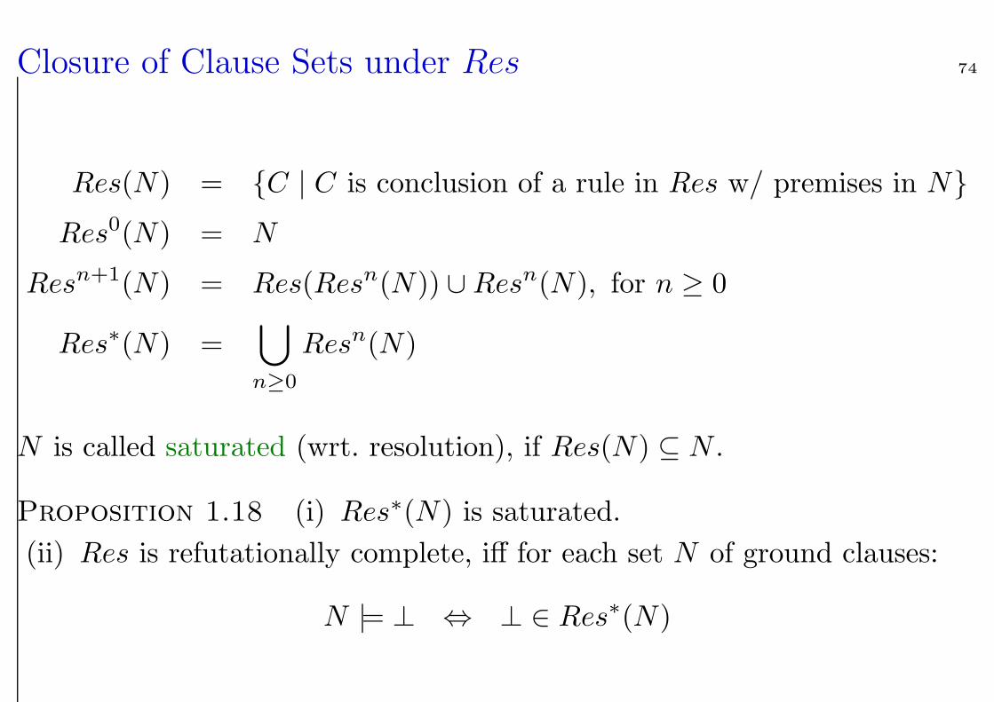
Closure of Clause Sets under Res 74
Res(N) = C | C is conclusion of a rule in Res w/ premises in N
Res0(N) = N
Resn+1(N) = Res(Resn(N)) ∪Resn(N), for n ≥ 0
Res∗(N) =⋃
n≥0
Resn(N)
N is called saturated (wrt. resolution), if Res(N) ⊆ N .
Proposition 1.18 (i) Res∗(N) is saturated.
(ii) Res is refutationally complete, iff for each set N of ground clauses:
N |= ⊥ ⇔ ⊥ ∈ Res∗(N)
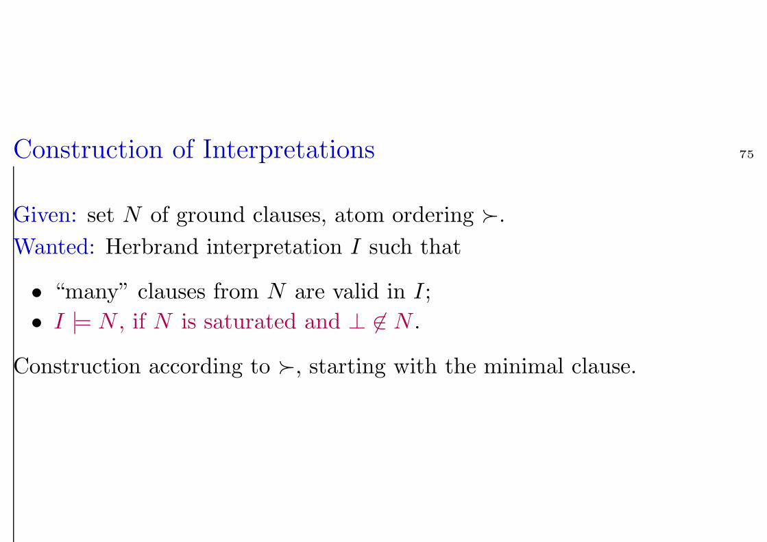
Construction of Interpretations 75
Given: set N of ground clauses, atom ordering .
Wanted: Herbrand interpretation I such that
• “many” clauses from N are valid in I;
• I |= N , if N is saturated and ⊥ 6∈ N .
Construction according to , starting with the minimal clause.
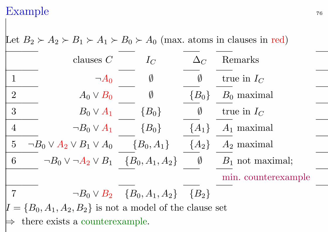
Example 76
Let B2 A2 B1 A1 B0 A0 (max. atoms in clauses in red)
clauses C IC ∆C Remarks
1 ¬A0 ∅ ∅ true in IC
2 A0 ∨B0 ∅ B0 B0 maximal
3 B0 ∨A1 B0 ∅ true in IC
4 ¬B0 ∨A1 B0 A1 A1 maximal
5 ¬B0 ∨A2 ∨B1 ∨A0 B0, A1 A2 A2 maximal
6 ¬B0 ∨ ¬A2 ∨B1 B0, A1, A2 ∅ B1 not maximal;
min. counterexample
7 ¬B0 ∨B2 B0, A1, A2 B2
I = B0, A1, A2, B2 is not a model of the clause set
⇒ there exists a counterexample.
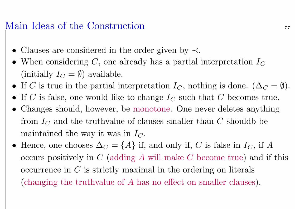
Main Ideas of the Construction 77
• Clauses are considered in the order given by ≺.
• When considering C, one already has a partial interpretation IC
(initially IC = ∅) available.
• If C is true in the partial interpretation IC , nothing is done. (∆C = ∅).
• If C is false, one would like to change IC such that C becomes true.
• Changes should, however, be monotone. One never deletes anything
from IC and the truthvalue of clauses smaller than C shouldb be
maintained the way it was in IC .
• Hence, one chooses ∆C = A if, and only if, C is false in IC , if A
occurs positively in C (adding A will make C become true) and if this
occurrence in C is strictly maximal in the ordering on literals
(changing the truthvalue of A has no effect on smaller clauses).

Resolution Reduces Counterexamples 78
¬B0 ∨A2 ∨B1 ∨A0 ¬B0 ∨ ¬A2 ∨B1
¬B0 ∨ ¬B0 ∨B1 ∨B1 ∨A0
Construction of I for the extended clause set:
clauses C IC ∆C
¬A0 ∅ ∅
A0 ∨ B0 ∅ B0
B0 ∨ A1 B0 ∅
¬B0 ∨ A1 B0 A1
¬B0 ∨ ¬B0 ∨ B1 ∨ B1 ∨ A0 B0, A1 ∅ B1 occurs twice
minimal counterexample
¬B0 ∨ A2 ∨ B1 ∨ A0 B0, A1 A2
¬B0 ∨ ¬A2 ∨ B1 B0, A1, A2 ∅ counterexample
¬B0 ∨ B2 B0, A1, A2 B2
The same I, but smaller counterexample, hence some progress was made.
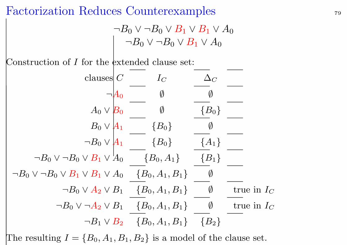
Factorization Reduces Counterexamples 79
¬B0 ∨ ¬B0 ∨B1 ∨B1 ∨A0
¬B0 ∨ ¬B0 ∨B1 ∨A0
Construction of I for the extended clause set:
clauses C IC ∆C
¬A0 ∅ ∅
A0 ∨ B0 ∅ B0
B0 ∨ A1 B0 ∅
¬B0 ∨ A1 B0 A1
¬B0 ∨ ¬B0 ∨ B1 ∨ A0 B0, A1 B1
¬B0 ∨ ¬B0 ∨ B1 ∨ B1 ∨ A0 B0, A1, B1 ∅
¬B0 ∨ A2 ∨ B1 B0, A1, B1 ∅ true in IC
¬B0 ∨ ¬A2 ∨ B1 B0, A1, B1 ∅ true in IC
¬B1 ∨ B2 B0, A1, B1 B2
The resulting I = B0, A1, B1, B2 is a model of the clause set.
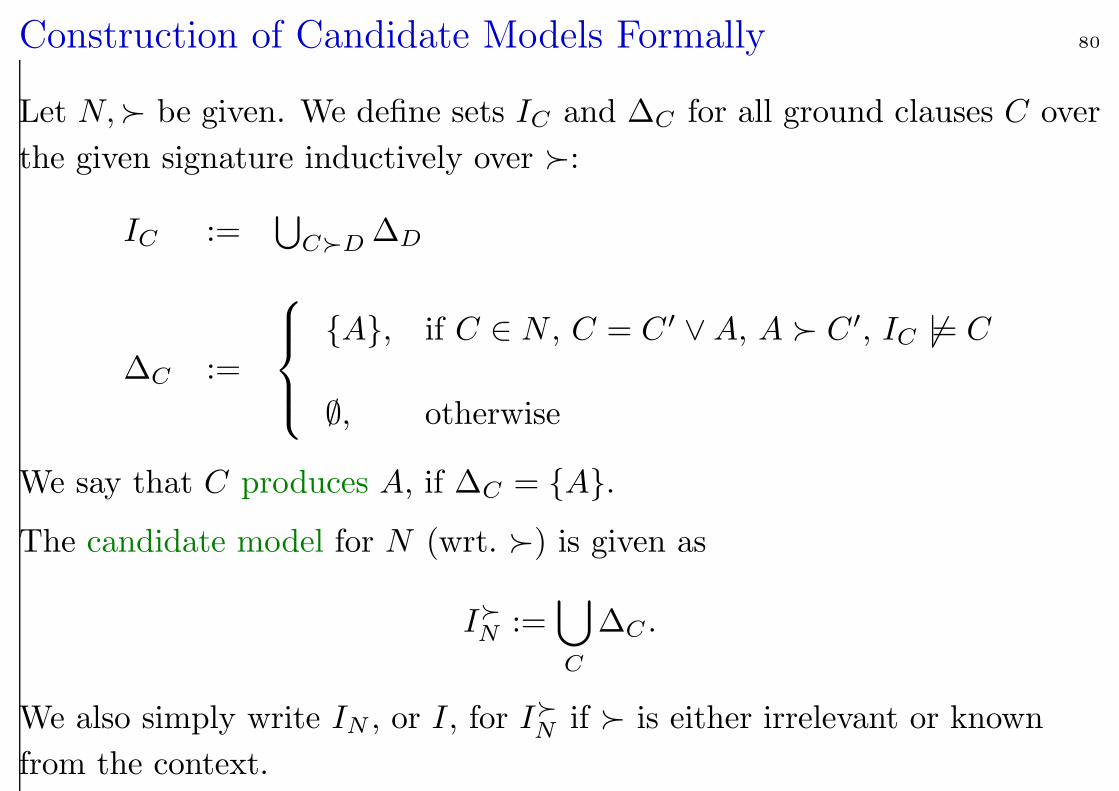
Construction of Candidate Models Formally 80
Let N, be given. We define sets IC and ∆C for all ground clauses C over
the given signature inductively over :
IC :=⋃
CD ∆D
∆C :=
A, if C ∈ N , C = C ′ ∨A, A C ′, IC 6|= C
∅, otherwise
We say that C produces A, if ∆C = A.
The candidate model for N (wrt. ) is given as
IN :=⋃
C
∆C .
We also simply write IN , or I, for IN if is either irrelevant or known
from the context.
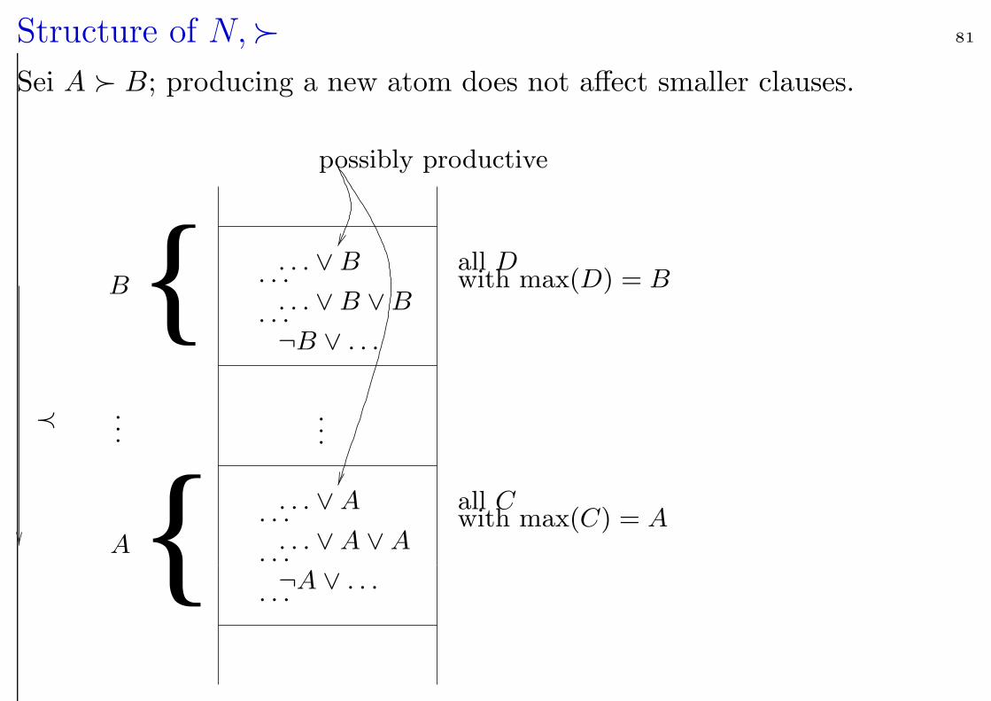
Structure of N, 81
Sei A B; producing a new atom does not affect smaller clauses.
PSfrag replacements
......
≺
possibly productive
A
B. . . ∨ B. . .. . . ∨ B ∨ B. . .¬B ∨ . . .
. . . ∨ A. . .
. . . ∨ A ∨ A. . .¬A ∨ . . .. . .
all Dwith max(D) = B
all Cwith max(C) = A
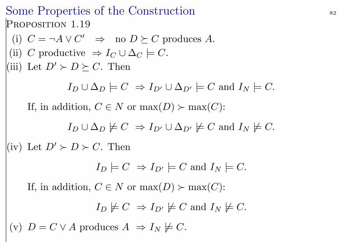
Some Properties of the Construction 82
Proposition 1.19
(i) C = ¬A ∨ C ′ ⇒ no D C produces A.
(ii) C productive ⇒ IC ∪∆C |= C.
(iii) Let D′ D C. Then
ID ∪∆D |= C ⇒ ID′ ∪∆D′ |= C and IN |= C.
If, in addition, C ∈ N or max(D) max(C):
ID ∪∆D 6|= C ⇒ ID′ ∪∆D′ 6|= C and IN 6|= C.
(iv) Let D′ D C. Then
ID |= C ⇒ ID′ |= C and IN |= C.
If, in addition, C ∈ N or max(D) max(C):
ID 6|= C ⇒ ID′ 6|= C and IN 6|= C.
(v) D = C ∨A produces A ⇒ IN 6|= C.
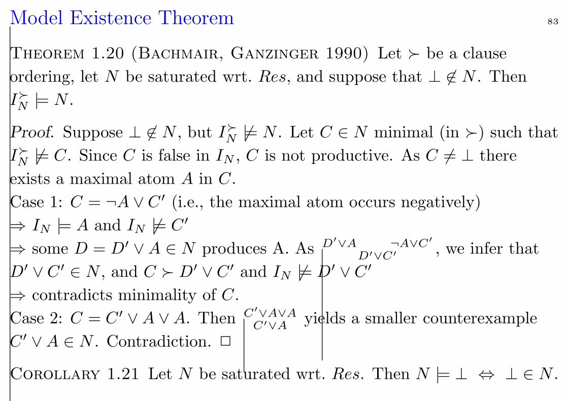
Model Existence Theorem 83
Theorem 1.20 (Bachmair, Ganzinger 1990) Let be a clause
ordering, let N be saturated wrt. Res, and suppose that ⊥ 6∈ N . Then
IN |= N .
Proof. Suppose ⊥ 6∈ N , but IN 6|= N . Let C ∈ N minimal (in ) such that
IN 6|= C. Since C is false in IN , C is not productive. As C 6= ⊥ there
exists a maximal atom A in C.
Case 1: C = ¬A ∨ C ′ (i.e., the maximal atom occurs negatively)
⇒ IN |= A and IN 6|= C ′
⇒ some D = D′ ∨A ∈ N produces A. As D′∨A ¬A∨C′
D′∨C′ , we infer that
D′ ∨ C ′ ∈ N , and C D′ ∨ C ′ and IN 6|= D′ ∨ C ′
⇒ contradicts minimality of C.
Case 2: C = C ′ ∨A ∨A. Then C′∨A∨AC′∨A yields a smaller counterexample
C ′ ∨A ∈ N . Contradiction. 2
Corollary 1.21 Let N be saturated wrt. Res. Then N |= ⊥ ⇔ ⊥ ∈ N .
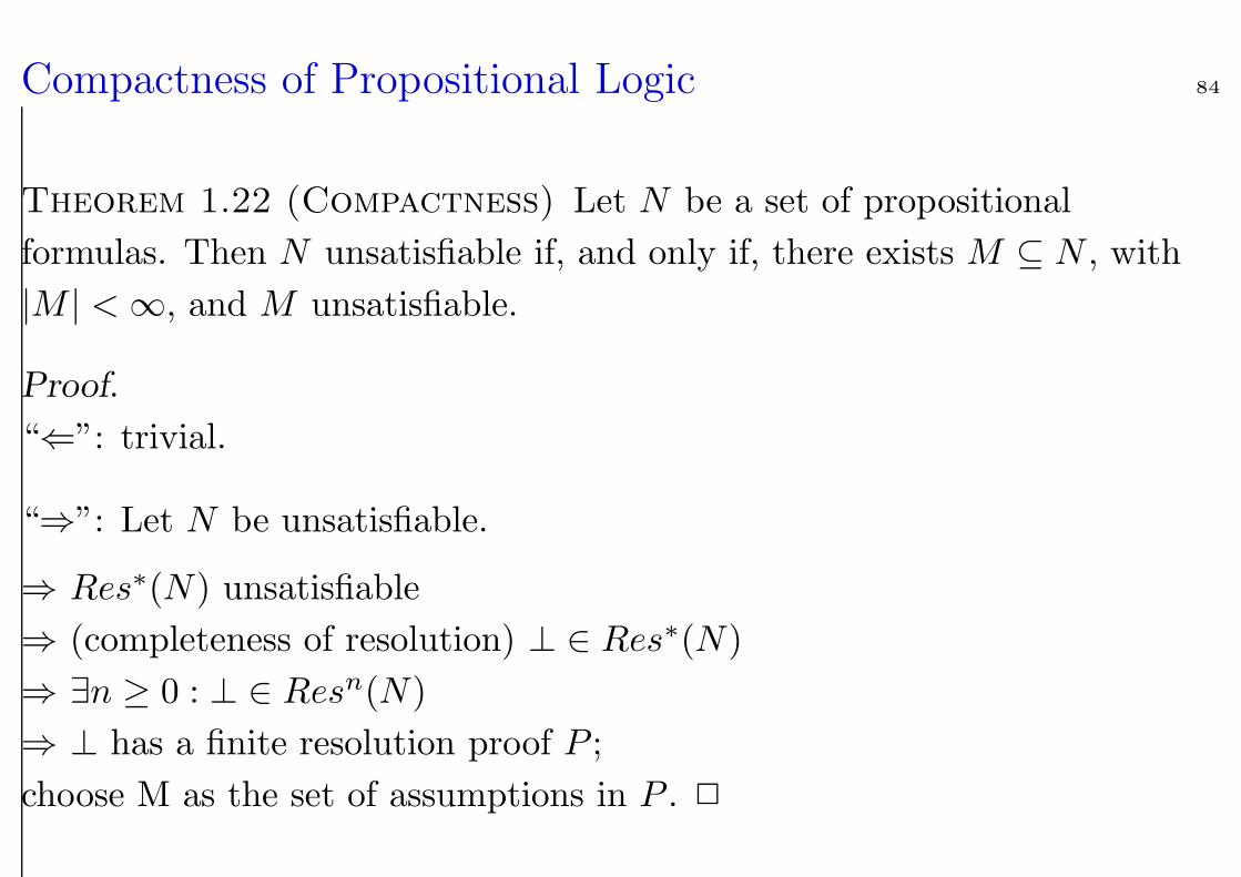
Compactness of Propositional Logic 84
Theorem 1.22 (Compactness) Let N be a set of propositional
formulas. Then N unsatisfiable if, and only if, there exists M ⊆ N , with
|M | <∞, and M unsatisfiable.
Proof.
“⇐”: trivial.
“⇒”: Let N be unsatisfiable.
⇒ Res∗(N) unsatisfiable
⇒ (completeness of resolution) ⊥ ∈ Res∗(N)
⇒ ∃n ≥ 0 : ⊥ ∈ Resn(N)
⇒ ⊥ has a finite resolution proof P ;
choose M as the set of assumptions in P . 2
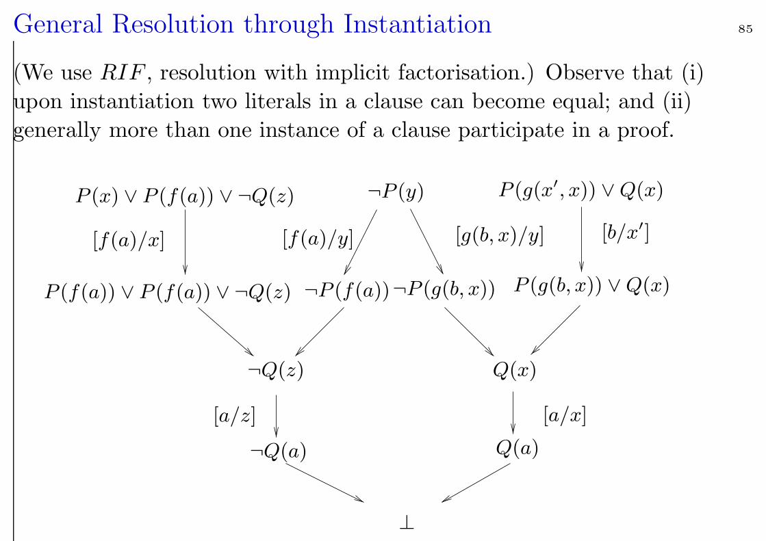
General Resolution through Instantiation 85
(We use RIF , resolution with implicit factorisation.) Observe that (i)
upon instantiation two literals in a clause can become equal; and (ii)
generally more than one instance of a clause participate in a proof.
PSfrag replacements
P (x) ∨ P (f(a)) ∨ ¬Q(z) ¬P (y) P (g(x′, x)) ∨ Q(x)
P (f(a)) ∨ P (f(a)) ∨ ¬Q(z) ¬P (f(a))¬P (g(b, x)) P (g(b, x)) ∨ Q(x)
¬Q(z)
¬Q(a)
Q(x)
Q(a)
⊥
[f(a)/x]
[a/z]
[f(a)/y] [g(b, x)/y] [b/x′]
[a/x]
Lifting Principle 86
Problem: Make saturation of infinite sets of clauses as they arise from
taking the (ground) instances of finitely many general clauses (with
variables) effective and efficient.
Idea (Robinson 65): • Resolution for general clauses• Equality of ground atoms is generalized to unifiability of general
atoms• Only compute most general (minimal) unfiers
Significance: The advantage of the method in (Robinson 65) compared
with (Gilmore 60) is that unification enumerates only those instances
of clauses that participate in an inference. Moreover, clauses are not
right away instantiated into ground clauses. Rather they are
instantiated only as far as required for an inference. Inferences with
non-ground clauses in general represent infinite sets of ground
inferences which are computed simultaneously in a single step.
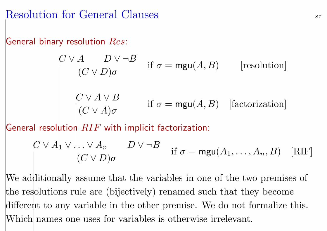
Resolution for General Clauses 87
General binary resolution Res:
C ∨A D ∨ ¬B
(C ∨D)σif σ = mgu(A,B) [resolution]
C ∨A ∨B
(C ∨A)σif σ = mgu(A,B) [factorization]
General resolution RIF with implicit factorization:
C ∨A1 ∨ . . . ∨An D ∨ ¬B
(C ∨D)σif σ = mgu(A1, . . . , An, B) [RIF]
We additionally assume that the variables in one of the two premises of
the resolutions rule are (bijectively) renamed such that they become
different to any variable in the other premise. We do not formalize this.
Which names one uses for variables is otherwise irrelevant.
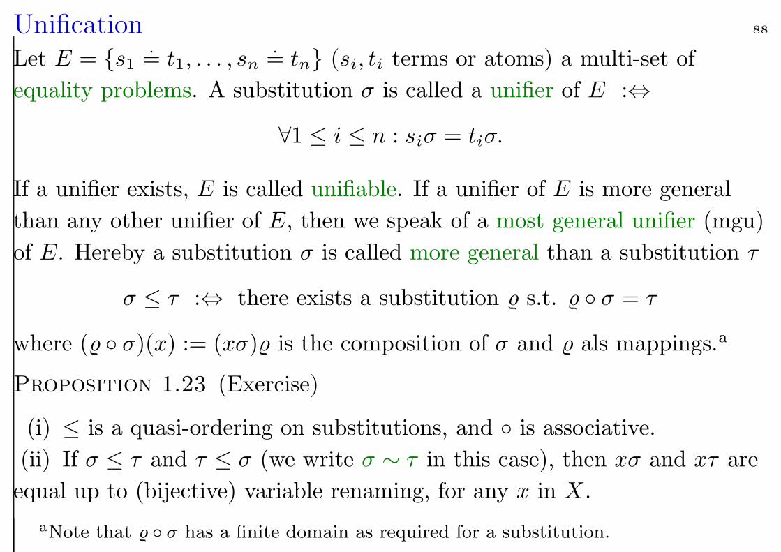
Unification 88
Let E = s1.= t1, . . . , sn
.= tn (si, ti terms or atoms) a multi-set of
equality problems. A substitution σ is called a unifier of E :⇔
∀1 ≤ i ≤ n : siσ = tiσ.
If a unifier exists, E is called unifiable. If a unifier of E is more general
than any other unifier of E, then we speak of a most general unifier (mgu)
of E. Hereby a substitution σ is called more general than a substitution τ
σ ≤ τ :⇔ there exists a substitution % s.t. % σ = τ
where (% σ)(x) := (xσ)% is the composition of σ and % als mappings.a
Proposition 1.23 (Exercise)
(i) ≤ is a quasi-ordering on substitutions, and is associative.
(ii) If σ ≤ τ and τ ≤ σ (we write σ ∼ τ in this case), then xσ and xτ are
equal up to (bijective) variable renaming, for any x in X.
aNote that % σ has a finite domain as required for a substitution.
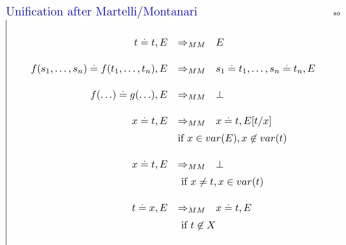
Unification after Martelli/Montanari 89
t.= t, E ⇒MM E
f(s1, . . . , sn).= f(t1, . . . , tn), E ⇒MM s1
.= t1, . . . , sn
.= tn, E
f(. . .).= g(. . .), E ⇒MM ⊥
x.= t, E ⇒MM x
.= t, E[t/x]
if x ∈ var(E), x 6∈ var(t)
x.= t, E ⇒MM ⊥
if x 6= t, x ∈ var(t)
t.= x,E ⇒MM x
.= t, E
if t 6∈ X
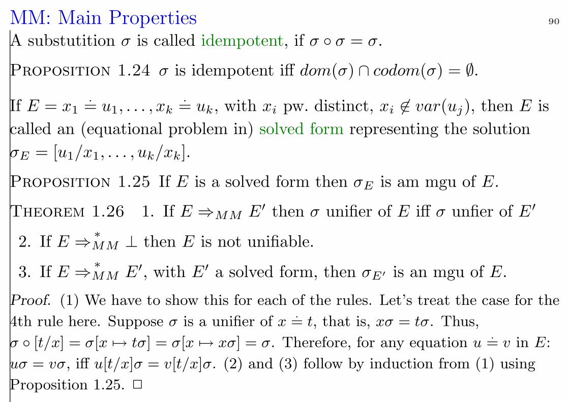
MM: Main Properties 90
A substutition σ is called idempotent, if σ σ = σ.
Proposition 1.24 σ is idempotent iff dom(σ) ∩ codom(σ) = ∅.
If E = x1
.= u1, . . . , xk
.= uk, with xi pw. distinct, xi 6∈ var(uj), then E is
called an (equational problem in) solved form representing the solution
σE = [u1/x1, . . . , uk/xk].
Proposition 1.25 If E is a solved form then σE is am mgu of E.
Theorem 1.26 1. If E ⇒MM E′ then σ unifier of E iff σ unfier of E ′
2. If E∗
⇒MM ⊥ then E is not unifiable.
3. If E∗
⇒MM E′, with E′ a solved form, then σE′ is an mgu of E.
Proof. (1) We have to show this for each of the rules. Let’s treat the case for the
4th rule here. Suppose σ is a unifier of x.= t, that is, xσ = tσ. Thus,
σ [t/x] = σ[x 7→ tσ] = σ[x 7→ xσ] = σ. Therefore, for any equation u.= v in E:
uσ = vσ, iff u[t/x]σ = v[t/x]σ. (2) and (3) follow by induction from (1) using
Proposition 1.25. 2
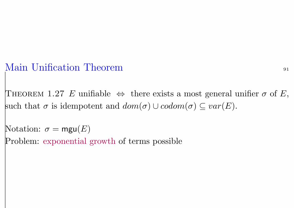
Main Unification Theorem 91
Theorem 1.27 E unifiable ⇔ there exists a most general unifier σ of E,
such that σ is idempotent and dom(σ) ∪ codom(σ) ⊆ var(E).
Notation: σ = mgu(E)
Problem: exponential growth of terms possible
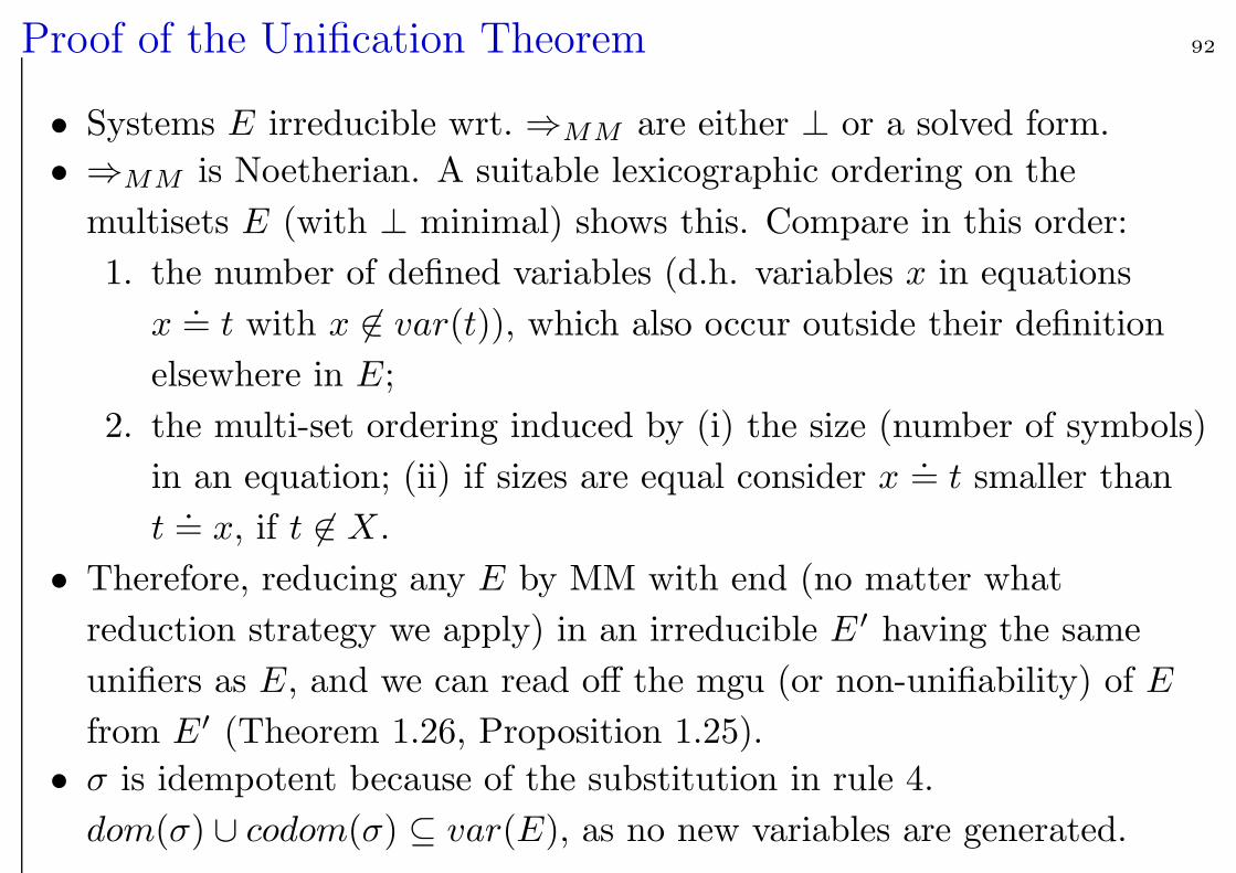
Proof of the Unification Theorem 92
• Systems E irreducible wrt. ⇒MM are either ⊥ or a solved form.
• ⇒MM is Noetherian. A suitable lexicographic ordering on the
multisets E (with ⊥ minimal) shows this. Compare in this order:
1. the number of defined variables (d.h. variables x in equations
x.= t with x 6∈ var(t)), which also occur outside their definition
elsewhere in E;
2. the multi-set ordering induced by (i) the size (number of symbols)
in an equation; (ii) if sizes are equal consider x.= t smaller than
t.= x, if t 6∈ X.
• Therefore, reducing any E by MM with end (no matter what
reduction strategy we apply) in an irreducible E ′ having the same
unifiers as E, and we can read off the mgu (or non-unifiability) of E
from E′ (Theorem 1.26, Proposition 1.25).
• σ is idempotent because of the substitution in rule 4.
dom(σ) ∪ codom(σ) ⊆ var(E), as no new variables are generated.
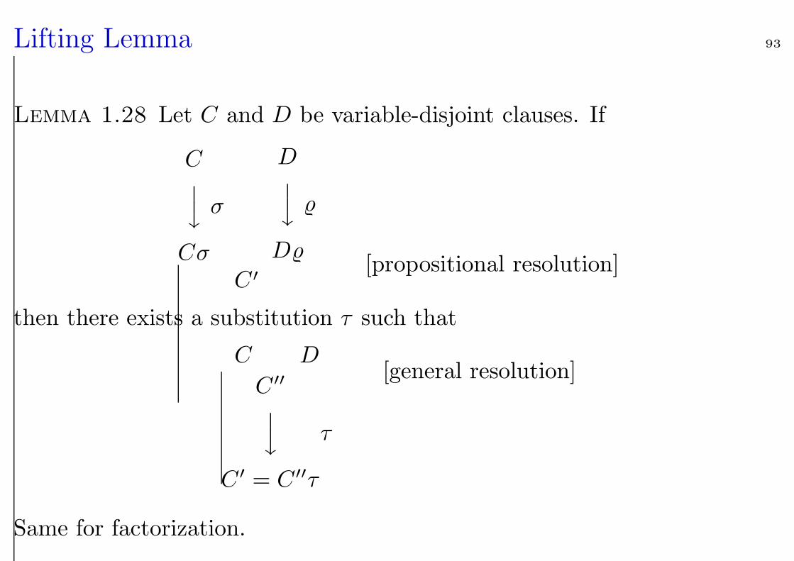
Lifting Lemma 93
Lemma 1.28 Let C and D be variable-disjoint clauses. If
Cy σ
Cσ
Dy %
D%
C ′[propositional resolution]
then there exists a substitution τ such that
C D
C ′′
y τ
C ′ = C ′′τ
[general resolution]
Same for factorization.
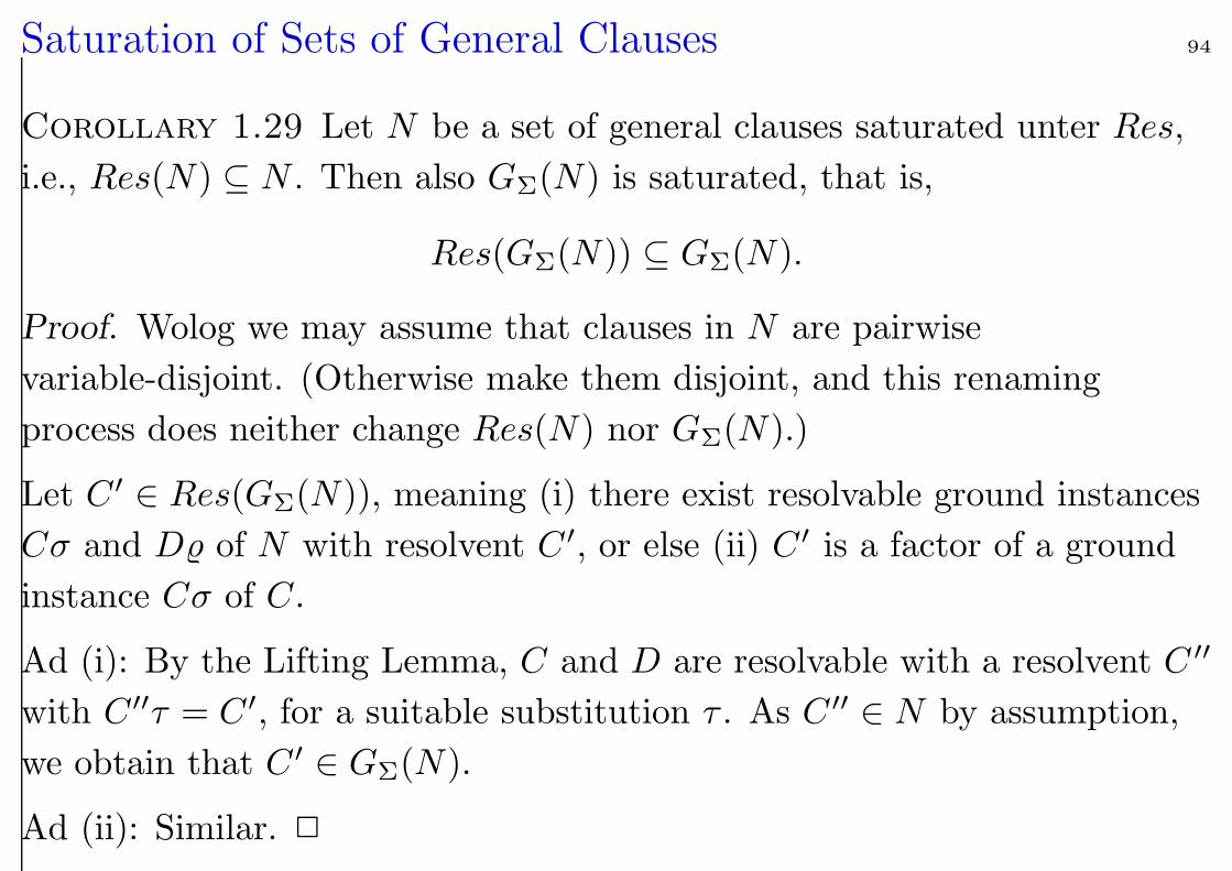
Saturation of Sets of General Clauses 94
Corollary 1.29 Let N be a set of general clauses saturated unter Res,
i.e., Res(N) ⊆ N . Then also GΣ(N) is saturated, that is,
Res(GΣ(N)) ⊆ GΣ(N).
Proof. Wolog we may assume that clauses in N are pairwise
variable-disjoint. (Otherwise make them disjoint, and this renaming
process does neither change Res(N) nor GΣ(N).)
Let C ′ ∈ Res(GΣ(N)), meaning (i) there exist resolvable ground instances
Cσ and D% of N with resolvent C ′, or else (ii) C ′ is a factor of a ground
instance Cσ of C.
Ad (i): By the Lifting Lemma, C and D are resolvable with a resolvent C ′′
with C ′′τ = C ′, for a suitable substitution τ . As C ′′ ∈ N by assumption,
we obtain that C ′ ∈ GΣ(N).
Ad (ii): Similar. 2
Herbrand’s Theorem 95
Theorem 1.30 (Herbrand) Let N be a set of Σ-clauses.
N satisfiable ⇔ N has a Herbrand model over Σ
Proof. “⇐”trivial
“⇒”
N 6|= ⊥ ⇒ ⊥ 6∈ Res∗(N) (resolution is sound)
⇒ ⊥ 6∈ GΣ(Res∗(N))
⇒ IGΣ(Res∗(N)) |= GΣ(Res∗(N)) (Theorem 1.20; Corollary 1.29)
⇒ IGΣ(Res∗(N)) |= Res∗(N) (I is a Herbrand model)
⇒ IGΣ(Res∗(N)) |= N (N ⊆ Res∗(N))
2
The Theorem of Lowenheim-Skolem 96
Theorem 1.31 (Lowenheim-Skolem) Let Σ be a countable signature
and let S be a set of closed Σ-formulas. Then S is satisfiable iff S has a
model over a countable universe.
Proof. S kann be at most countably infinite if both X and Σ are countable. Now
generate, maintaining satisfiability, a set N of clauses from S. This extends Σ by
at most countably many new Skolem functions to Σ′. As Σ′ is countable, so is
TΣ′ , the universe of Herbrand-interpretations over Σ′. Now apply Thereom 1.30.
2
Refutational Completeness of General Resolution 97
Theorem 1.32 Let N be a set of general clauses where Res(N) ⊆ N .
Then
N |= ⊥ ⇔ ⊥ ∈ N.
Proof. Let Res(N) ⊆ N . By Corollary 1.29: Res(GΣ(N)) ⊆ GΣ(N)
N |= ⊥ ⇔ GΣ(N) |= ⊥ (Theorem 1.30)
⇔ ⊥ ∈ GΣ(N) (propositional resolution sound and complete)
⇔ ⊥ ∈ N
2
Compactness of Predicate Logic 98
Theorem 1.33 (Compactness Theorem for First-Order Logic)
Let Φ be a set of first-order Formulas. Φ unsatisfiable ⇔ there exists
Ψ ⊆ Φ, |Ψ| <∞, Ψ unsatisfiable.
Proof.
“⇐”: trivial.
“⇒”: Let Φ be unsatisfiable and let N be the set of clauses obtained by
Skolemization and CNF transformation of the formulas in Φ.
⇒ Res∗(N) unsatisfiable
⇒ (Thm 1.32) ⊥ ∈ Res∗(N)
⇒ ∃n ≥ 0 : ⊥ ∈ Resn(N)
⇒ ⊥ has finite resolution proof B of depth ≤ n.
Choose Ψ als the subset of formulas in Φ such that the corresponding
clauses contain the assumptions (leaves) of B. 2
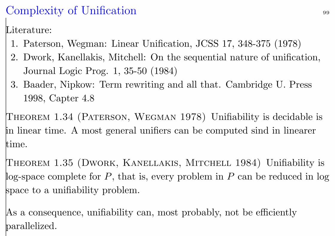
Complexity of Unification 99
Literature:
1. Paterson, Wegman: Linear Unification, JCSS 17, 348-375 (1978)
2. Dwork, Kanellakis, Mitchell: On the sequential nature of unification,
Journal Logic Prog. 1, 35-50 (1984)
3. Baader, Nipkow: Term rewriting and all that. Cambridge U. Press
1998, Capter 4.8
Theorem 1.34 (Paterson, Wegman 1978) Unifiability is decidable is
in linear time. A most general unifiers can be computed sind in linearer
time.
Theorem 1.35 (Dwork, Kanellakis, Mitchell 1984) Unifiability is
log-space complete for P , that is, every problem in P can be reduced in log
space to a unifiability problem.
As a consequence, unifiability can, most probably, not be efficiently
parallelized.
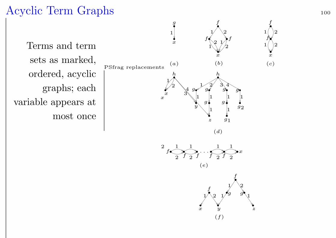
Acyclic Term Graphs 100
Terms and term
sets as marked,
ordered, acyclic
graphs; each
variable appears at
most once
PSfrag replacements
gg
gggg
gg
g
f
f
fffff
ff
f f
f
hh
x
x
x
x
x
x
x
y
y
z
z g1
g2
1
1
11
1 1 1 1
1
111 1
1
11
11
11
1
1
2
2
2
2 222
22
22
2
2
2
3
3
44
(a) (b) (c)
(d)
(e)
(f)
. . .
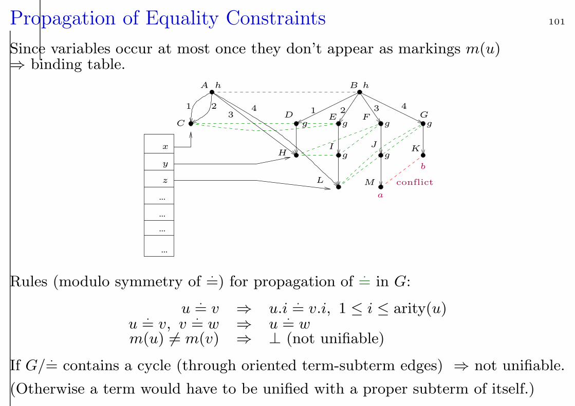
Propagation of Equality Constraints 101
Since variables occur at most once they don’t appear as markings m(u)⇒ binding table.
...
...
...
...
PSfrag replacements
A B
CD E F G
HI J
K
L M
hh
gg
g g g g
x
y
z
a
b
conflict
11 22 33
44
Rules (modulo symmetry of.=) for propagation of
.= in G:
u.= v ⇒ u.i
.= v.i, 1 ≤ i ≤ arity(u)
u.= v, v
.= w ⇒ u
.= w
m(u) 6= m(v) ⇒ ⊥ (not unifiable)
If G/.= contains a cycle (through oriented term-subterm edges) ⇒ not unifiable.
(Otherwise a term would have to be unified with a proper subterm of itself.)
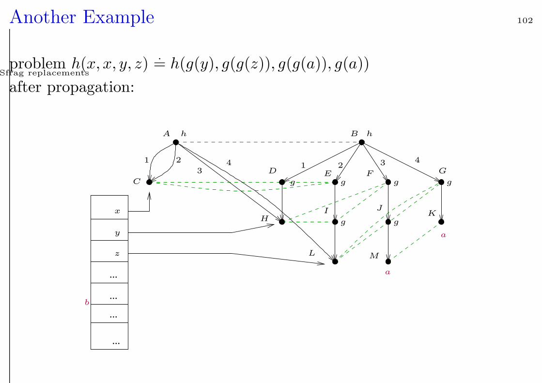
Another Example 102
problem h(x, x, y, z).= h(g(y), g(g(z)), g(g(a)), g(a))
after propagation:
...
...
...
...
PSfrag replacements
A B
C
D E F G
HI J
K
L M
hh
gg
g g g g
x
y
z
a
a
b
11
22 3
3
44
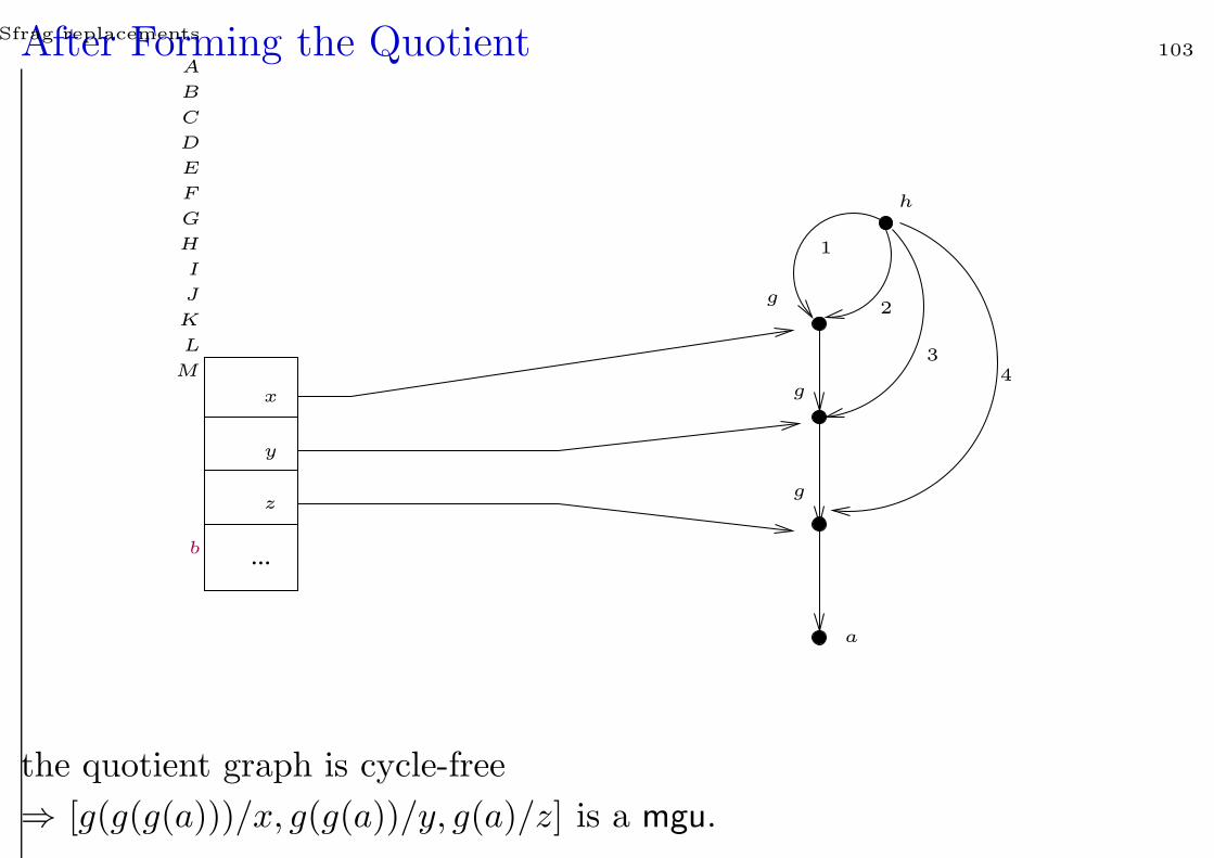
After Forming the Quotient 103
...
PSfrag replacements
A
B
C
D
E
F
G
H
I
J
K
L
M
h
g
g
gx
y
z
a
b
1
2
34
the quotient graph is cycle-free
⇒ [g(g(g(a)))/x, g(g(a))/y, g(a)/z] is a mgu.
Analysis 104
For a unification problem with term graph of size n we obtain without
much effort these complexity bounds:
• additional space in O(log2n)
• runtime in O(n3)
In fact, at most n2 edges can be generated by propagation, and each of
those requires time O(n) for a reachability test. For the quotient we have
to compute the strongly connected components and then do the cycle test.
This is both possible in time linear in the size of the graph, that is, in
O(n2).
Matching 105
Let s, t be terms or atoms.
s matches t :
s ≤ t :⇔ there exists a substitution σ s.t. sσ = t
(σ is called a matching substitution.)
s ≤ t ⇒ σ = mgu(s, t), if var(t) ∩ var(s) = ∅.
Theorem 1.36 (Dwork, Kanellakis, Mitchell 1984) Matching can
be efficiently parallelized.
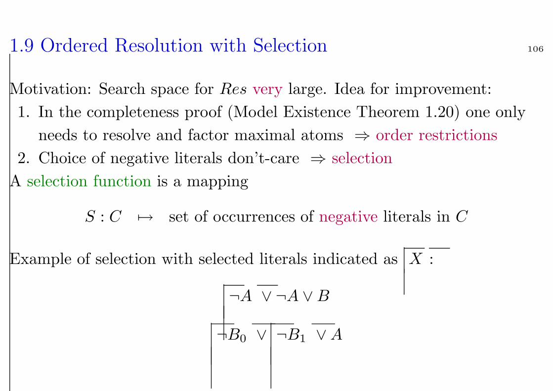
1.9 Ordered Resolution with Selection 106
Motivation: Search space for Res very large. Idea for improvement:
1. In the completeness proof (Model Existence Theorem 1.20) one only
needs to resolve and factor maximal atoms ⇒ order restrictions
2. Choice of negative literals don’t-care ⇒ selection
A selection function is a mapping
S : C 7→ set of occurrences of negative literals in C
Example of selection with selected literals indicated as X :
¬A ∨ ¬A ∨B
¬B0 ∨ ¬B1 ∨A
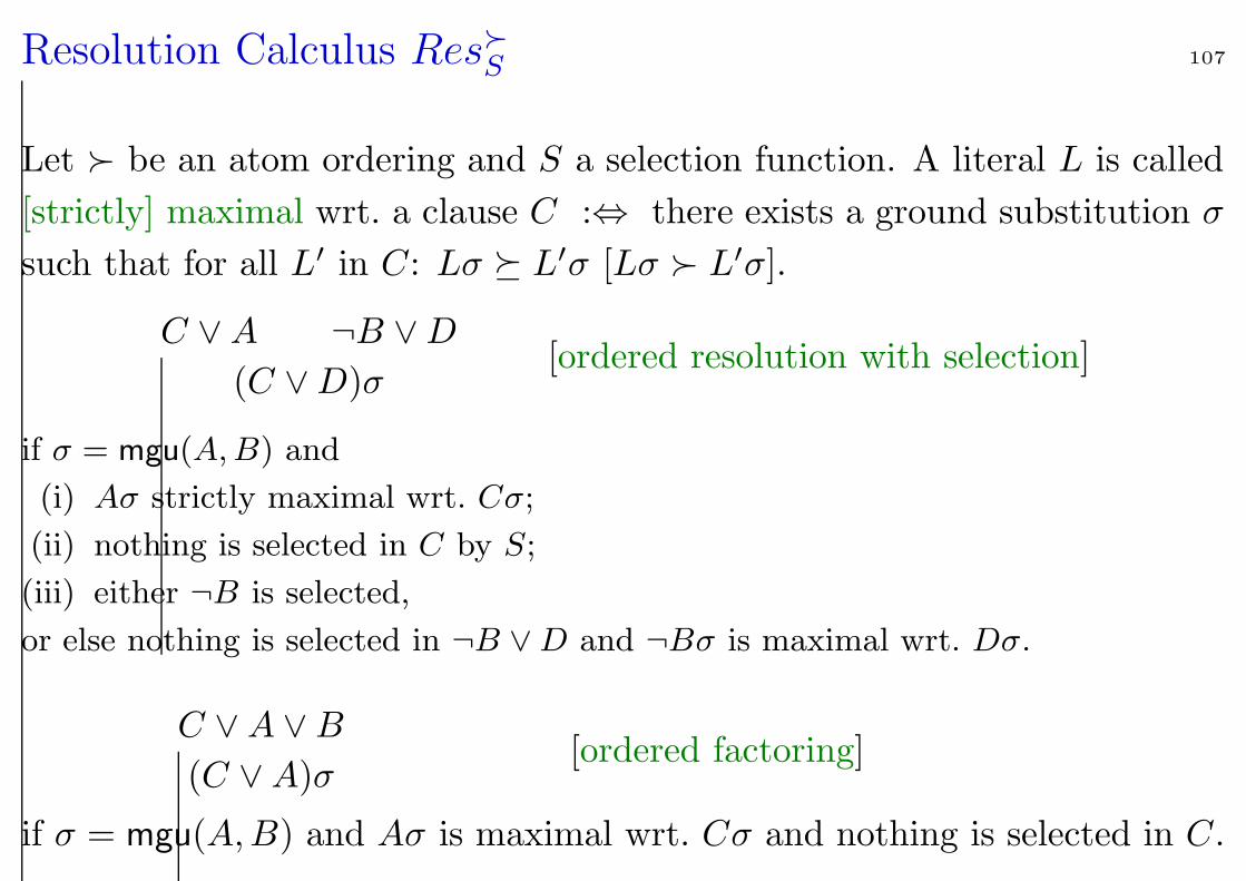
Resolution Calculus ResS 107
Let be an atom ordering and S a selection function. A literal L is called
[strictly] maximal wrt. a clause C :⇔ there exists a ground substitution σ
such that for all L′ in C: Lσ L′σ [Lσ L′σ].
C ∨A ¬B ∨D
(C ∨D)σ[ordered resolution with selection]
if σ = mgu(A, B) and
(i) Aσ strictly maximal wrt. Cσ;
(ii) nothing is selected in C by S;
(iii) either ¬B is selected,
or else nothing is selected in ¬B ∨ D and ¬Bσ is maximal wrt. Dσ.
C ∨A ∨B
(C ∨A)σ[ordered factoring]
if σ = mgu(A,B) and Aσ is maximal wrt. Cσ and nothing is selected in C.
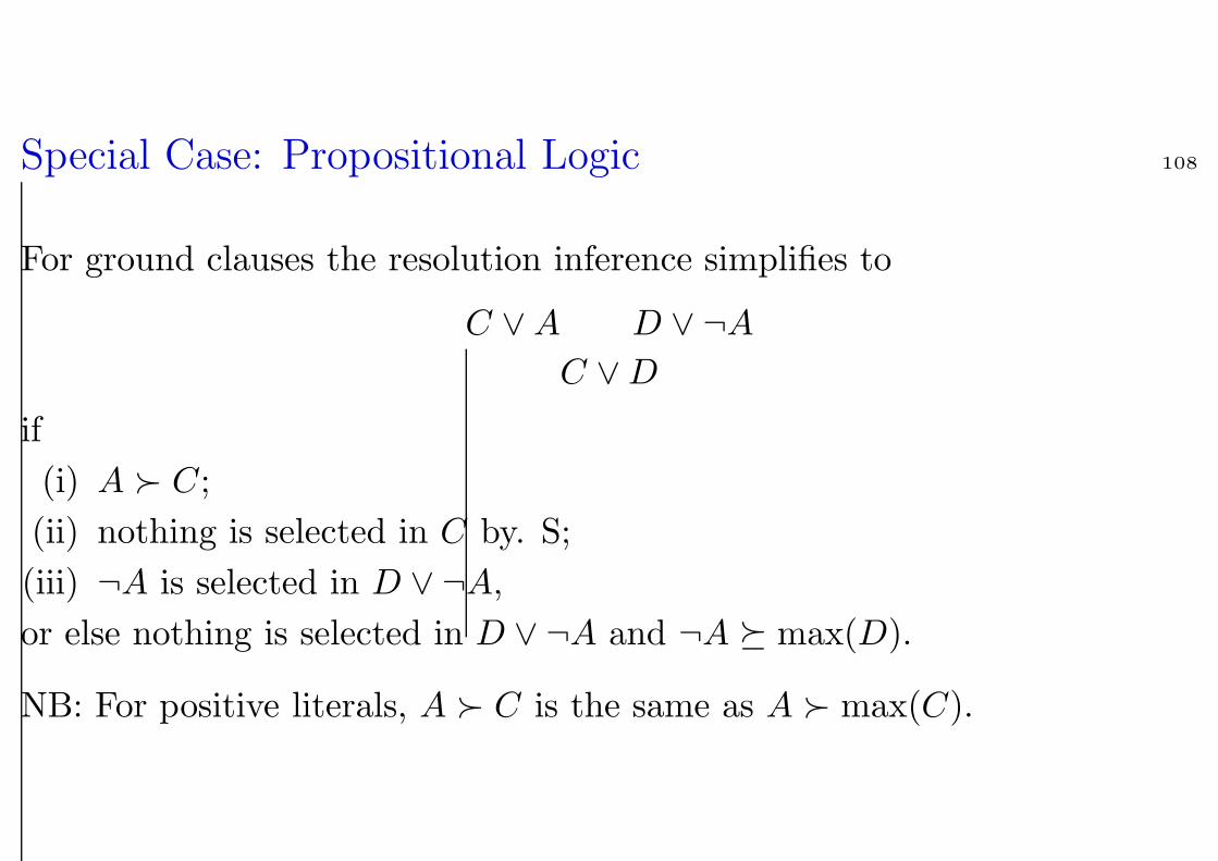
Special Case: Propositional Logic 108
For ground clauses the resolution inference simplifies to
C ∨A D ∨ ¬A
C ∨D
if
(i) A C;
(ii) nothing is selected in C by. S;
(iii) ¬A is selected in D ∨ ¬A,
or else nothing is selected in D ∨ ¬A and ¬A max(D).
NB: For positive literals, A C is the same as A max(C).
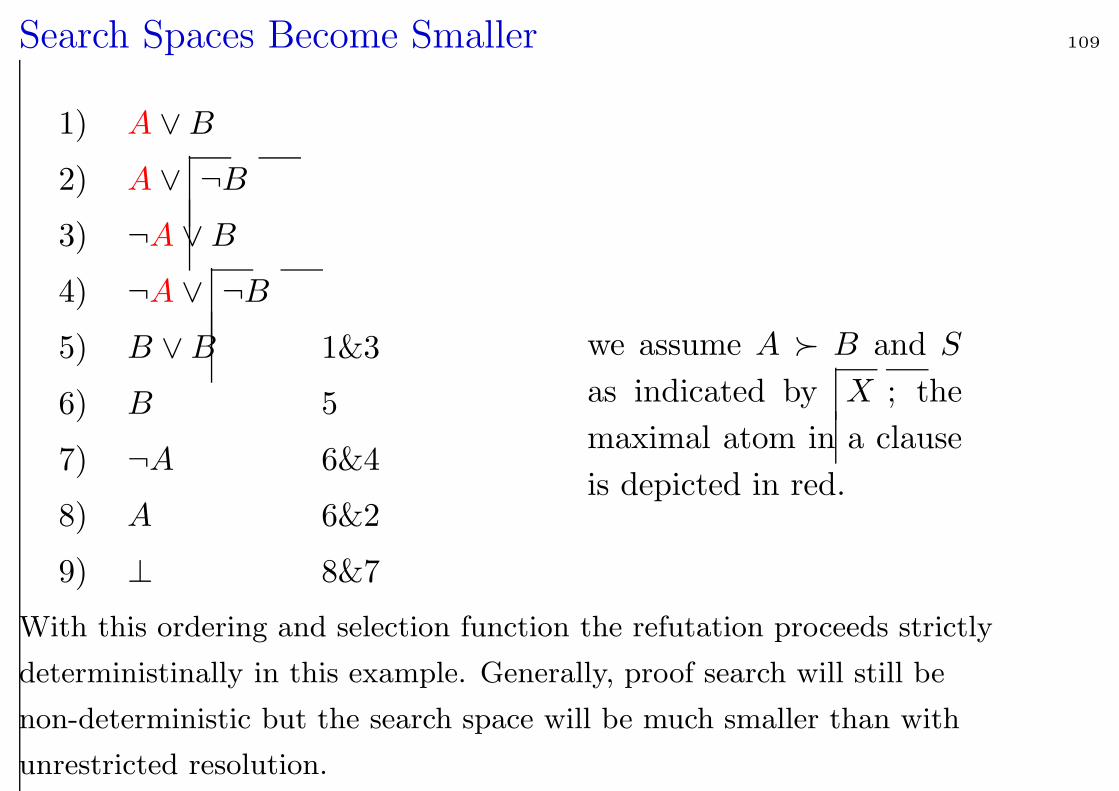
Search Spaces Become Smaller 109
1) A ∨B
2) A ∨ ¬B
3) ¬A ∨B
4) ¬A ∨ ¬B
5) B ∨B 1&3
6) B 5
7) ¬A 6&4
8) A 6&2
9) ⊥ 8&7
we assume A B and S
as indicated by X ; the
maximal atom in a clause
is depicted in red.
With this ordering and selection function the refutation proceeds strictly
deterministinally in this example. Generally, proof search will still be
non-deterministic but the search space will be much smaller than with
unrestricted resolution.
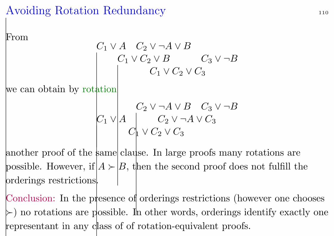
Avoiding Rotation Redundancy 110
FromC1 ∨A C2 ∨ ¬A ∨B
C1 ∨ C2 ∨B C3 ∨ ¬B
C1 ∨ C2 ∨ C3
we can obtain by rotation
C1 ∨A
C2 ∨ ¬A ∨B C3 ∨ ¬B
C2 ∨ ¬A ∨ C3
C1 ∨ C2 ∨ C3
another proof of the same clause. In large proofs many rotations are
possible. However, if A B, then the second proof does not fulfill the
orderings restrictions.
Conclusion: In the presence of orderings restrictions (however one chooses
) no rotations are possible. In other words, orderings identify exactly one
representant in any class of of rotation-equivalent proofs.
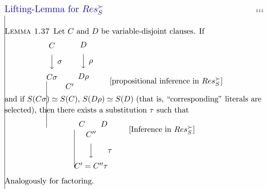
Lifting-Lemma for ResS 111
Lemma 1.37 Let C and D be variable-disjoint clauses. If
Cy σ
Cσ
Dy ρ
Dρ
C ′[propositional inference in ResS ]
and if S(Cσ) ' S(C), S(Dρ) ' S(D) (that is, “corresponding” literals are
selected), then there exists a substitution τ such that
C D
C ′′
y τ
C ′ = C ′′τ
[Inference in ResS ]
Analogously for factoring.
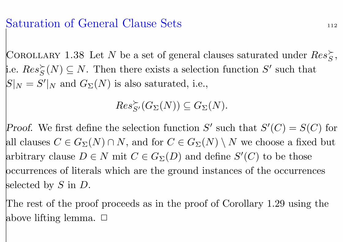
Saturation of General Clause Sets 112
Corollary 1.38 Let N be a set of general clauses saturated under ResS ,
i.e. ResS (N) ⊆ N . Then there exists a selection function S ′ such that
S|N = S′|N and GΣ(N) is also saturated, i.e.,
ResS′(GΣ(N)) ⊆ GΣ(N).
Proof. We first define the selection function S ′ such that S′(C) = S(C) for
all clauses C ∈ GΣ(N) ∩N , and for C ∈ GΣ(N) \N we choose a fixed but
arbitrary clause D ∈ N mit C ∈ GΣ(D) and define S′(C) to be those
occurrences of literals which are the ground instances of the occurrences
selected by S in D.
The rest of the proof proceeds as in the proof of Corollary 1.29 using the
above lifting lemma. 2
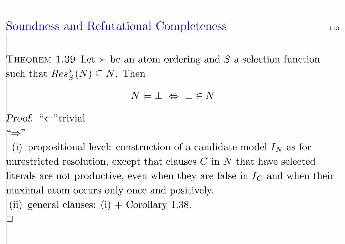
Soundness and Refutational Completeness 113
Theorem 1.39 Let be an atom ordering and S a selection function
such that ResS (N) ⊆ N . Then
N |= ⊥ ⇔ ⊥ ∈ N
Proof. “⇐”trivial
“⇒”
(i) propositional level: construction of a candidate model IN as for
unrestricted resolution, except that clauses C in N that have selected
literals are not productive, even when they are false in IC and when their
maximal atom occurs only once and positively.
(ii) general clauses: (i) + Corollary 1.38.
2
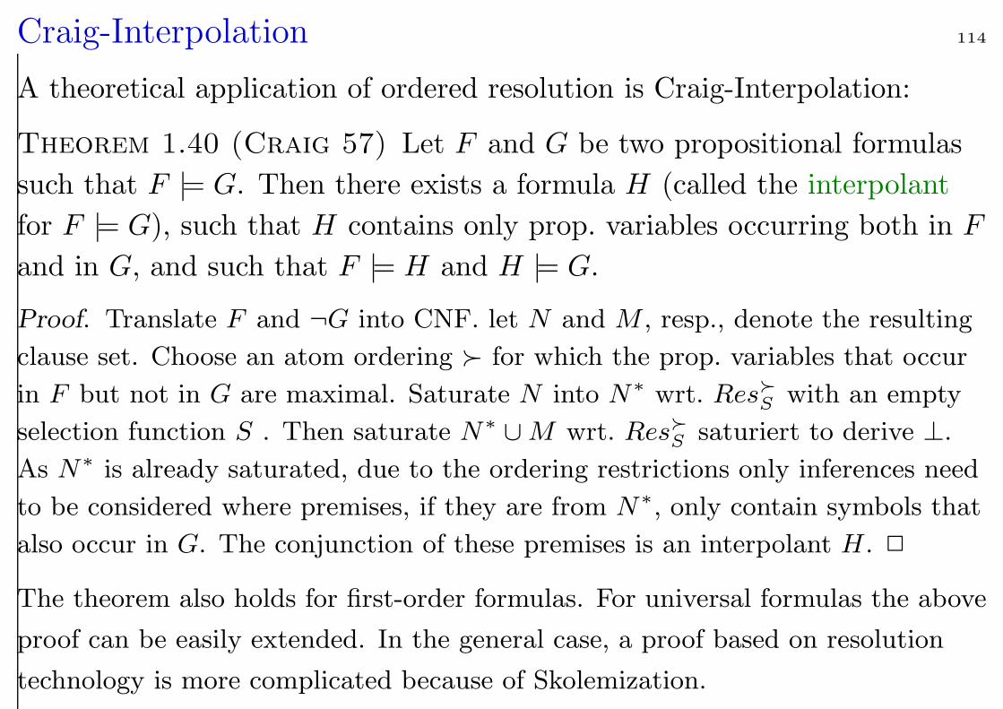
Craig-Interpolation 114
A theoretical application of ordered resolution is Craig-Interpolation:
Theorem 1.40 (Craig 57) Let F and G be two propositional formulas
such that F |= G. Then there exists a formula H (called the interpolant
for F |= G), such that H contains only prop. variables occurring both in F
and in G, and such that F |= H and H |= G.
Proof. Translate F and ¬G into CNF. let N and M , resp., denote the resulting
clause set. Choose an atom ordering for which the prop. variables that occur
in F but not in G are maximal. Saturate N into N∗ wrt. ResS
with an empty
selection function S . Then saturate N∗ ∪ M wrt. ResS
saturiert to derive ⊥.
As N∗ is already saturated, due to the ordering restrictions only inferences need
to be considered where premises, if they are from N∗, only contain symbols that
also occur in G. The conjunction of these premises is an interpolant H. 2
The theorem also holds for first-order formulas. For universal formulas the above
proof can be easily extended. In the general case, a proof based on resolution
technology is more complicated because of Skolemization.
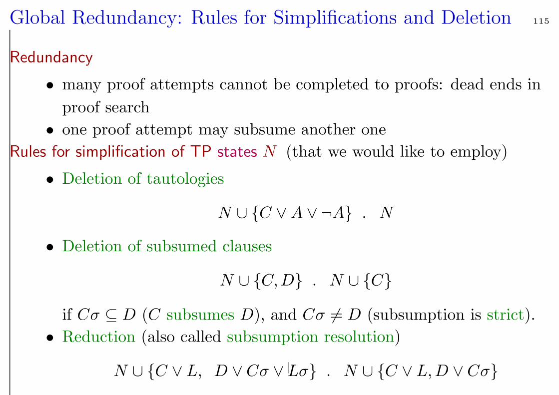
Global Redundancy: Rules for Simplifications and Deletion 115
Redundancy
• many proof attempts cannot be completed to proofs: dead ends in
proof search
• one proof attempt may subsume another one
Rules for simplification of TP states N (that we would like to employ)
• Deletion of tautologies
N ∪ C ∨A ∨ ¬A . N
• Deletion of subsumed clauses
N ∪ C,D . N ∪ C
if Cσ ⊆ D (C subsumes D), and Cσ 6= D (subsumption is strict).
• Reduction (also called subsumption resolution)
N ∪ C ∨ L, D ∨ Cσ ∨ Lσ . N ∪ C ∨ L,D ∨ Cσ
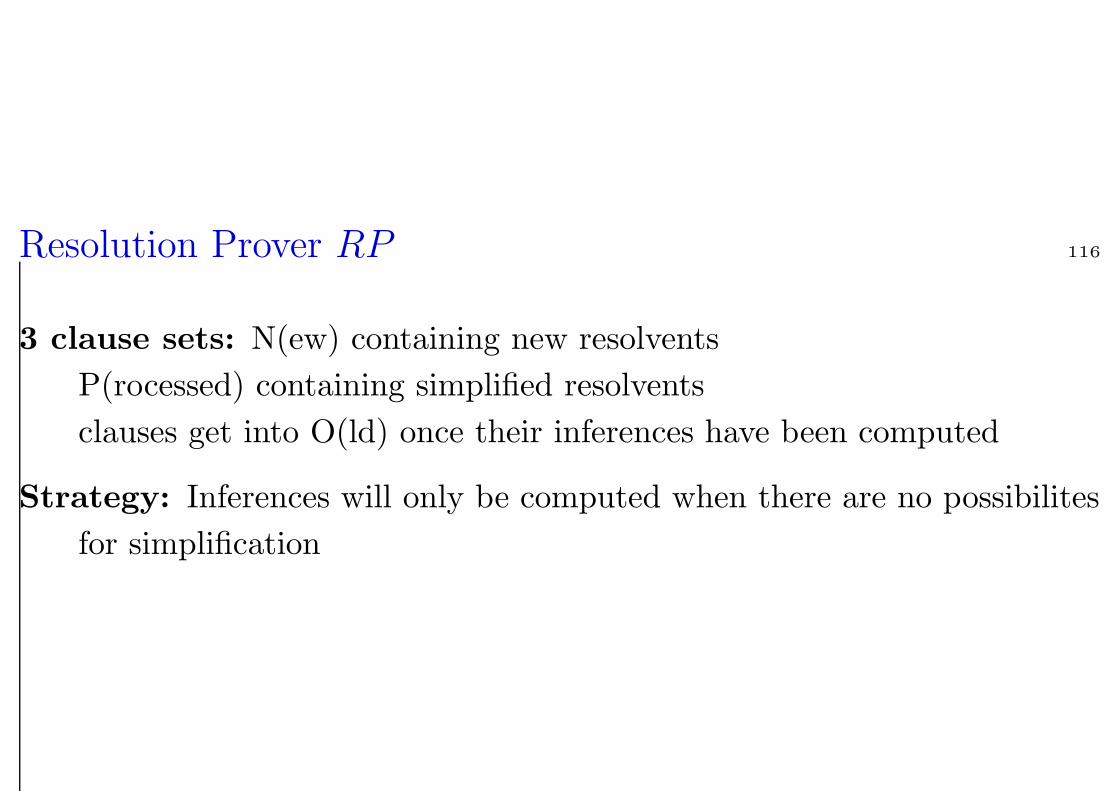
Resolution Prover RP 116
3 clause sets: N(ew) containing new resolvents
P(rocessed) containing simplified resolvents
clauses get into O(ld) once their inferences have been computed
Strategy: Inferences will only be computed when there are no possibilites
for simplification
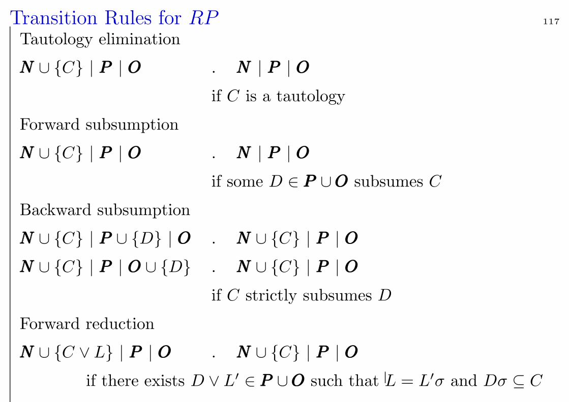
Transition Rules for RP 117
Tautology elimination
NNN ∪ C | PPP | OOO . NNN | PPP | OOO
if C is a tautology
Forward subsumption
NNN ∪ C | PPP | OOO . NNN | PPP | OOO
if some D ∈ PPP ∪OOO subsumes C
Backward subsumption
NNN ∪ C | PPP ∪ D | OOO . NNN ∪ C | PPP | OOO
NNN ∪ C | PPP | OOO ∪ D . NNN ∪ C | PPP | OOO
if C strictly subsumes D
Forward reduction
NNN ∪ C ∨ L | PPP | OOO . NNN ∪ C | PPP | OOO
if there exists D ∨ L′ ∈ PPP ∪OOO such that L = L′σ and Dσ ⊆ C
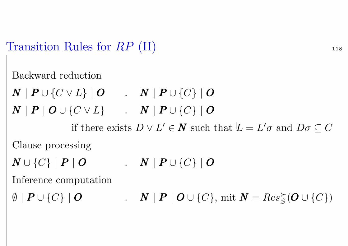
Transition Rules for RP (II) 118
Backward reduction
NNN | PPP ∪ C ∨ L | OOO . NNN | PPP ∪ C | OOO
NNN | PPP | OOO ∪ C ∨ L . NNN | PPP ∪ C | OOO
if there exists D ∨ L′ ∈NNN such that L = L′σ and Dσ ⊆ C
Clause processing
NNN ∪ C | PPP | OOO . NNN | PPP ∪ C | OOO
Inference computation
∅ | PPP ∪ C | OOO . NNN | PPP | OOO ∪ C, mit NNN = ResS (OOO ∪ C)
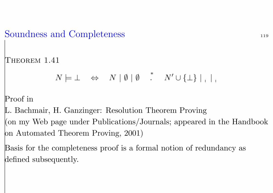
Soundness and Completeness 119
Theorem 1.41
N |= ⊥ ⇔ N | ∅ | ∅∗. N ′ ∪ ⊥ | |
Proof in
L. Bachmair, H. Ganzinger: Resolution Theorem Proving
(on my Web page under Publications/Journals; appeared in the Handbook
on Automated Theorem Proving, 2001)
Basis for the completeness proof is a formal notion of redundancy as
defined subsequently.
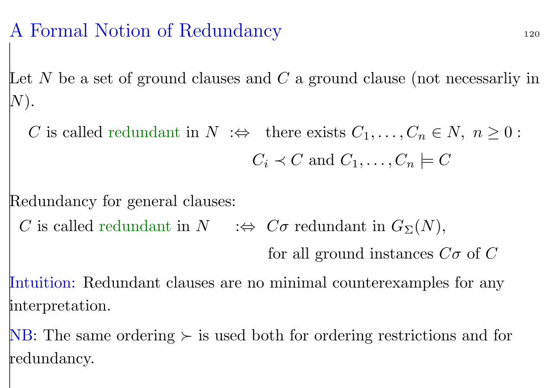
A Formal Notion of Redundancy 120
Let N be a set of ground clauses and C a ground clause (not necessarliy in
N).
C is called redundant in N :⇔ there exists C1, . . . , Cn ∈ N, n ≥ 0 :
Ci ≺ C and C1, . . . , Cn |= C
Redundancy for general clauses:
C is called redundant in N :⇔ Cσ redundant in GΣ(N),
for all ground instances Cσ of C
Intuition: Redundant clauses are no minimal counterexamples for any
interpretation.
NB: The same ordering is used both for ordering restrictions and for
redundancy.
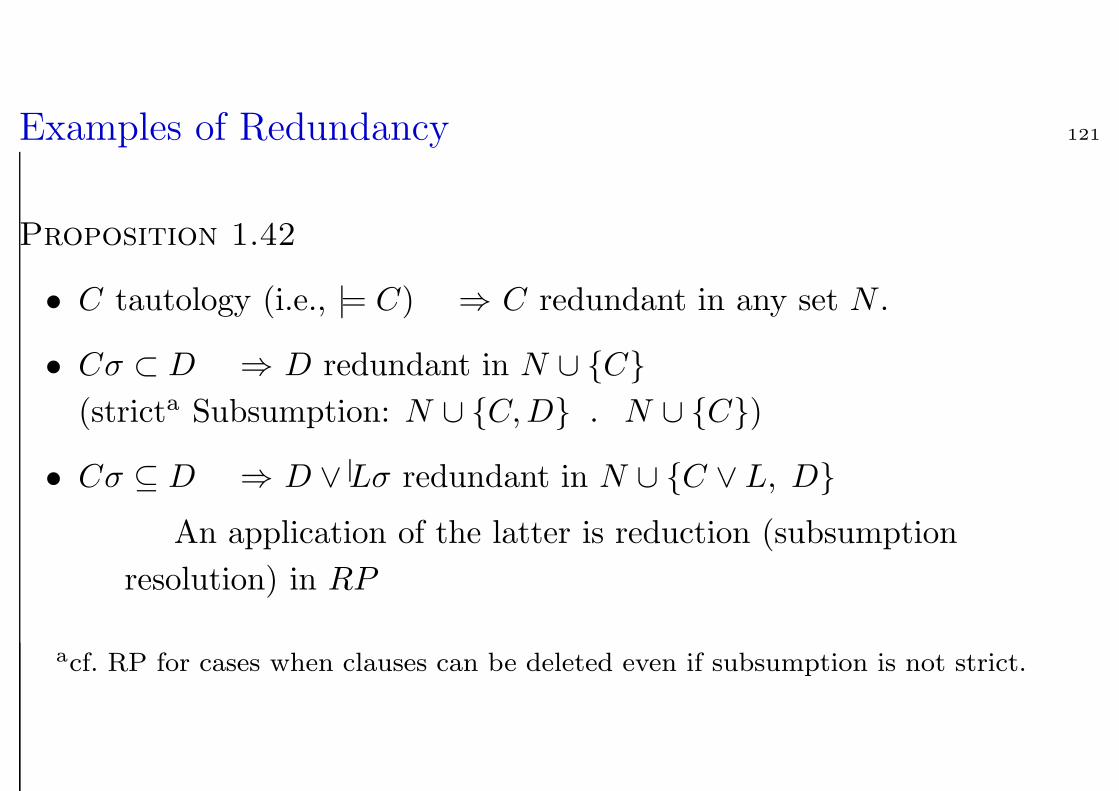
Examples of Redundancy 121
Proposition 1.42
• C tautology (i.e., |= C) ⇒ C redundant in any set N .
• Cσ ⊂ D ⇒ D redundant in N ∪ C
(stricta Subsumption: N ∪ C,D . N ∪ C)
• Cσ ⊆ D ⇒ D ∨ Lσ redundant in N ∪ C ∨ L, D
An application of the latter is reduction (subsumption
resolution) in RP
acf. RP for cases when clauses can be deleted even if subsumption is not strict.
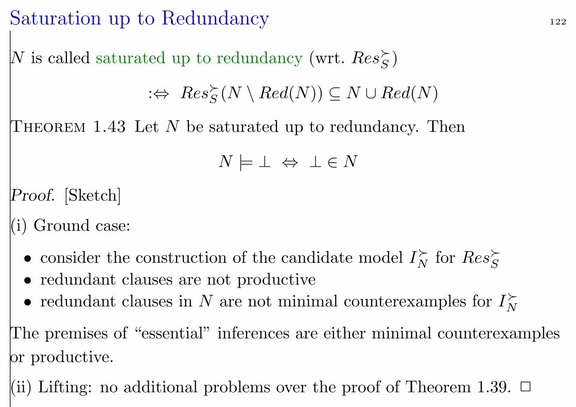
Saturation up to Redundancy 122
N is called saturated up to redundancy (wrt. ResS )
:⇔ ResS (N \Red(N)) ⊆ N ∪Red(N)
Theorem 1.43 Let N be saturated up to redundancy. Then
N |= ⊥ ⇔ ⊥ ∈ N
Proof. [Sketch]
(i) Ground case:
• consider the construction of the candidate model IN for ResS
• redundant clauses are not productive
• redundant clauses in N are not minimal counterexamples for IN
The premises of “essential” inferences are either minimal counterexamples
or productive.
(ii) Lifting: no additional problems over the proof of Theorem 1.39. 2
Monotonicity Properties of Redundancy 123
Theorem 1.44 (i) N ⊆M ⇒ Red(N) ⊆ Red(M)
(ii) M ⊆ Red(N) ⇒ Red(N) ⊆ Red(N \M)
Proof: Exercise.
We conclude that redundancy is preserved when, during a theorem proving
process, one adds (derives) new clauses or deletes redundant clauses.
The theorems 1.43 and 1.44 are the basis for the completeness proof of our
prover RP .
Hyperresolution (Robinson 65) 124
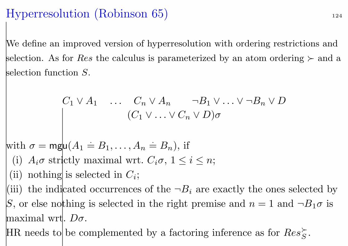
We define an improved version of hyperresolution with ordering restrictions and
selection. As for Res the calculus is parameterized by an atom ordering and a
selection function S.
C1 ∨A1 . . . Cn ∨An ¬B1 ∨ . . . ∨ ¬Bn ∨D
(C1 ∨ . . . ∨ Cn ∨D)σ
with σ = mgu(A1.= B1, . . . , An
.= Bn), if
(i) Aiσ strictly maximal wrt. Ciσ, 1 ≤ i ≤ n;
(ii) nothing is selected in Ci;
(iii) the indicated occurrences of the ¬Bi are exactly the ones selected by
S, or else nothing is selected in the right premise and n = 1 and ¬B1σ is
maximal wrt. Dσ.
HR needs to be complemented by a factoring inference as for ResS .
Hyperresolution (ctnd) 125
Hyperresolution can be simulated by iterated binary resolution. However
this yields intermediate clauses which HR might not derive, and many of
them might not be extendable into a full HR inference.
There are many more variants of resolution.
We refer to [Bachmair, Ganzinger: Resolution Theorem Proving] for
further reading.
1.10 Example: Neuman-Stubblebine Key Exchange Protocol 126
• Formalisation of a concrete application
• State-of-the-art in automated theorem proving
• Proof by consistency:
consistency ⇒ no unsafe states exist
• Termination requires elimination of redundancy
The Problem 127
Automatic Analysis of Security Protocols using SPASS: An Automated
Theorem Prover for First-Order Logic with Equality
by Christoph Weidenbach
The growing importance of the internet causes a growing need for security
protocols that protect transactions and communication. It turns out that the
design of such protocols is highly error-prone. Therefore, there is a need for tools
that automatically detect flaws like, e.g., attacks by an intruder. Here we show
that our automated theorem prover SPASS can successfully be used to analyze
the Newman-Stubblebine [1] key exchange protocol. To this end the protocol is
formalized in logic and then the security properties are automatically analyzed
by SPASS. A detailed description of the analysis can be found in [2]. The
animation successively shows two runs of the Newman-Stubblebine [1] key
exchange protocol. The first run works the way the protocol is designed to do,
i.e., it establishes a secure key between Alice and Bob.
The Problem (ctnd) 128
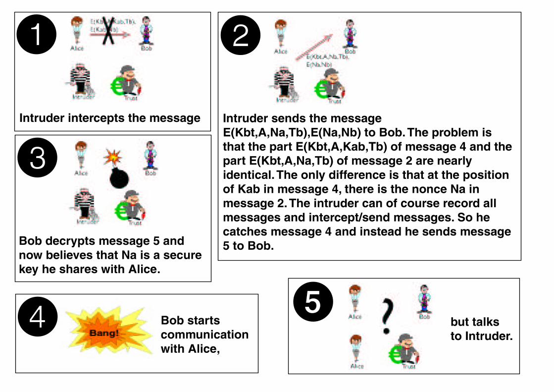
The second run shows a potential problem of the protocol. An intruder may
intercept the final message sent from Alice to Bob, replace it with a different
message and may eventually own a key that Bob believes to be a secure key with
Alice. The initial situation for the protocol is that the two participants Alice and
Bob want to establish a secure key for communication among them. They do so
with the help of a trusted server Trust where both already have a secure key for
communication with Trust. The below picture shows a sequence of four message
exchanges that eventually establishes the key.
! #" $ "
&%
'
' '
(
" )
"
! " $
#"
'
"
" "
" *
! #" $ ! " $
"
'
'
*
"
! #" $
'
'
! #" $
! $ *
'
' "
) '
' " '
" % '
! $
+
)
'
"
,
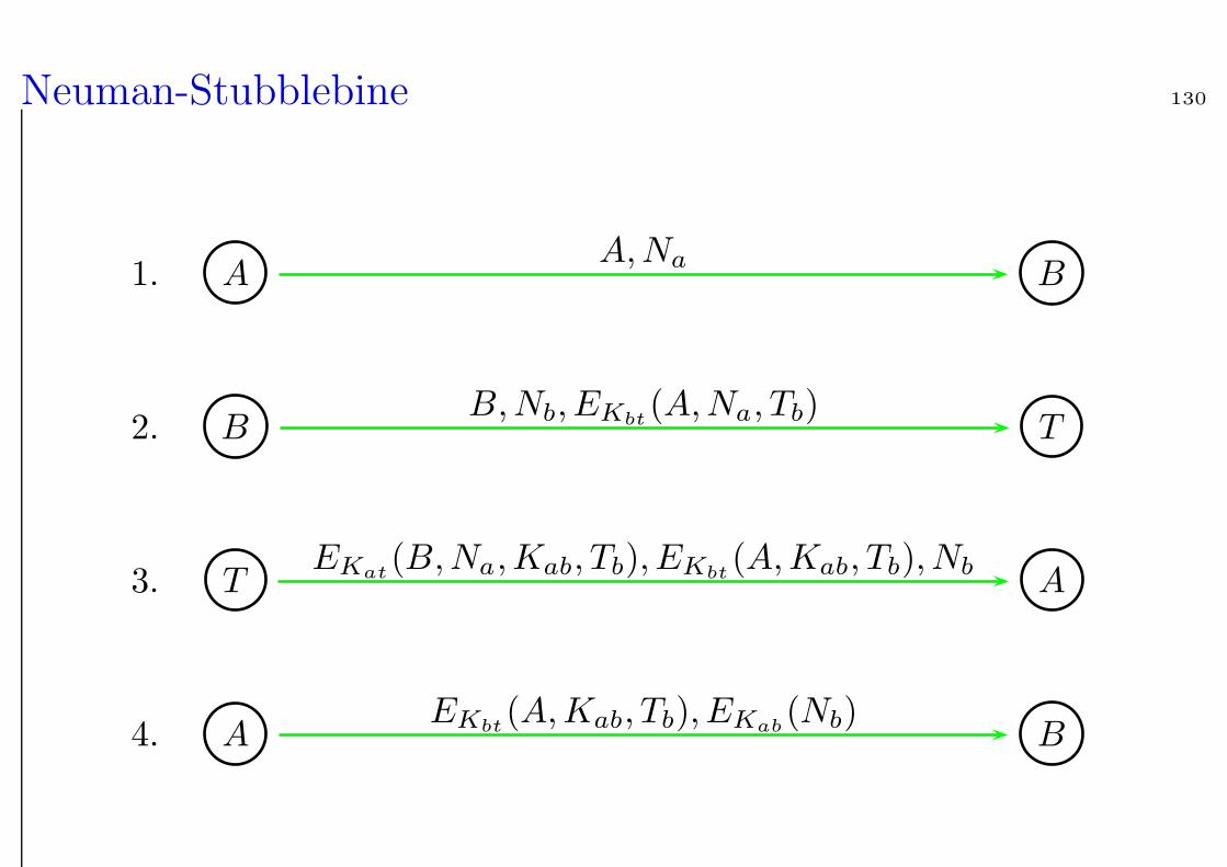
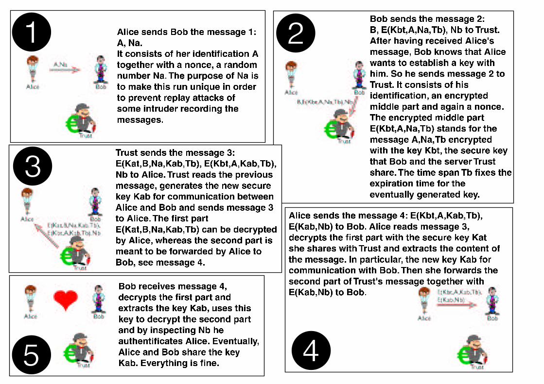
Neuman-Stubblebine 130
1. AA,Na B
2. BB,Nb, EKbt
(A,Na, Tb) T
3. TEKat
(B,Na,Kab, Tb), EKbt(A,Kab, Tb), Nb A
4. AEKbt
(A,Kab, Tb), EKab(Nb) B
What can happen? 131
How can an intruder now break this protocol? The key Kab is only
transmitted inside encrypted parts of messages and we assume that an
intruder cannot break any keys nor does he know any of the initial keys
Kat or Kbt. Here is the solution:
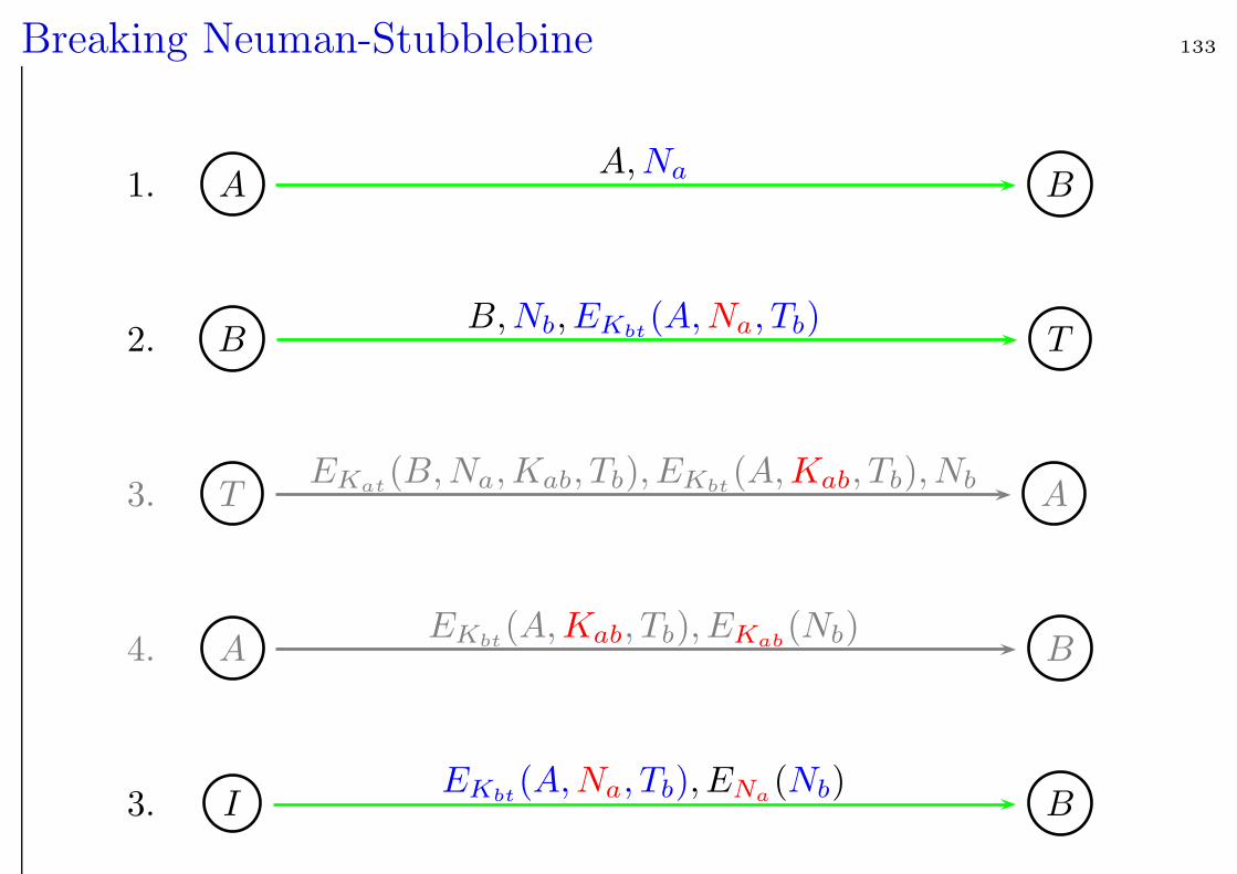
Breaking Neuman-Stubblebine 133
1. AA,Na B
2. BB,Nb, EKbt
(A,Na, Tb) T
3. TEKat
(B,Na,Kab, Tb), EKbt(A,Kab, Tb), Nb A
4. AEKbt
(A,Kab, Tb), EKab(Nb) B
3. IEKbt
(A,Na, Tb), ENa(Nb) B
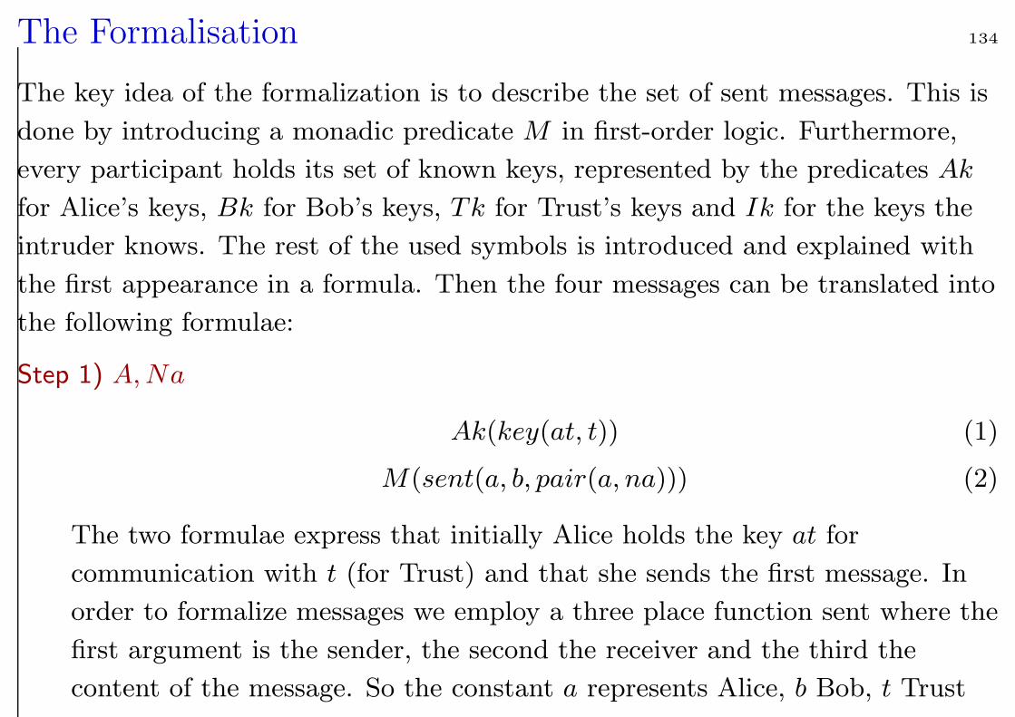
The Formalisation 134
The key idea of the formalization is to describe the set of sent messages. This is
done by introducing a monadic predicate M in first-order logic. Furthermore,
every participant holds its set of known keys, represented by the predicates Ak
for Alice’s keys, Bk for Bob’s keys, Tk for Trust’s keys and Ik for the keys the
intruder knows. The rest of the used symbols is introduced and explained with
the first appearance in a formula. Then the four messages can be translated into
the following formulae:
Step 1) A, Na
Ak(key(at, t)) (1)
M(sent(a, b, pair(a, na))) (2)
The two formulae express that initially Alice holds the key at for
communication with t (for Trust) and that she sends the first message. In
order to formalize messages we employ a three place function sent where the
first argument is the sender, the second the receiver and the third the
content of the message. So the constant a represents Alice, b Bob, t Trust
and i Intruder. The functions pair (triple, quadr) simply form sequences of
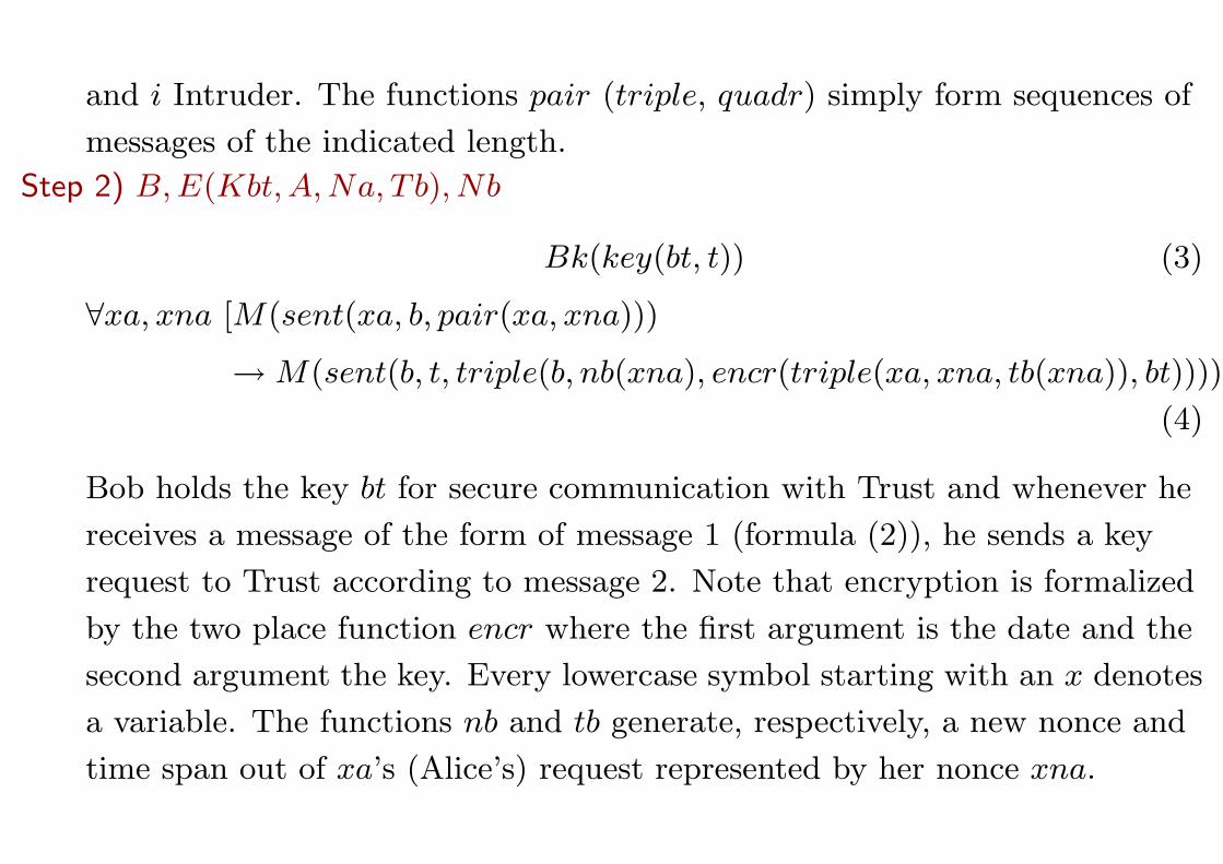
messages of the indicated length.
Step 2) B, E(Kbt, A, Na, T b), Nb
Bk(key(bt, t)) (3)
∀xa, xna [M(sent(xa, b, pair(xa, xna)))
→ M(sent(b, t, triple(b, nb(xna), encr(triple(xa, xna, tb(xna)), bt)))))]
(4)
Bob holds the key bt for secure communication with Trust and whenever he
receives a message of the form of message 1 (formula (2)), he sends a key
request to Trust according to message 2. Note that encryption is formalized
by the two place function encr where the first argument is the date and the
second argument the key. Every lowercase symbol starting with an x denotes
a variable. The functions nb and tb generate, respectively, a new nonce and
time span out of xa’s (Alice’s) request represented by her nonce xna.

Step 3) E(Kat, B, Na, Kab, T b), E(Kbt, A, Kab, T b), Nb
Tk(key(at, a))) ∧ Tk(key(bt, b)) (5)
∀xb, xnb,xa, xna, xbet, xbt, xat, xk
[ (M(sent(xb, t, triple(xb, xnb, encr(triple(xa, xna, xbet), xbt))))
∧ Tk(key(xbt, xb))
∧ Tk(key(xat, xa)))
→ M(sent(t, xa, triple(encr(quadr(xb, xna, kt(xna), xbet), xat),
encr(triple(xa, kt(xna), xbet), xbt), xnb))) ]
(6)
Trust holds the keys for Alice and Bob and answers appropriately to a
message in the format of message 2. Note that decryption is formalized by
unification with an appropriate term structure where it is checked that the
necessary keys are known to Trust. The server generates the key by
applying his key generation function kt to the nonce xna.
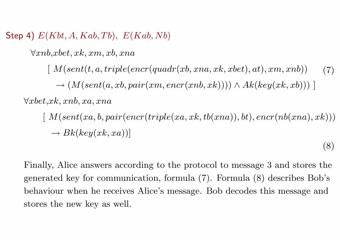
Step 4) E(Kbt, A, Kab, T b), E(Kab, Nb)
∀xnb,xbet, xk, xm, xb, xna
[ M(sent(t, a, triple(encr(quadr(xb, xna, xk, xbet), at), xm, xnb))
→ (M(sent(a, xb, pair(xm, encr(xnb, xk)))) ∧ Ak(key(xk, xb))) ]
(7)
∀xbet,xk, xnb, xa, xna
[ M(sent(xa, b, pair(encr(triple(xa, xk, tb(xna)), bt), encr(nb(xna), xk)))
→ Bk(key(xk, xa))]
(8)
Finally, Alice answers according to the protocol to message 3 and stores the
generated key for communication, formula (7). Formula (8) describes Bob’s
behaviour when he receives Alice’s message. Bob decodes this message and
stores the new key as well.
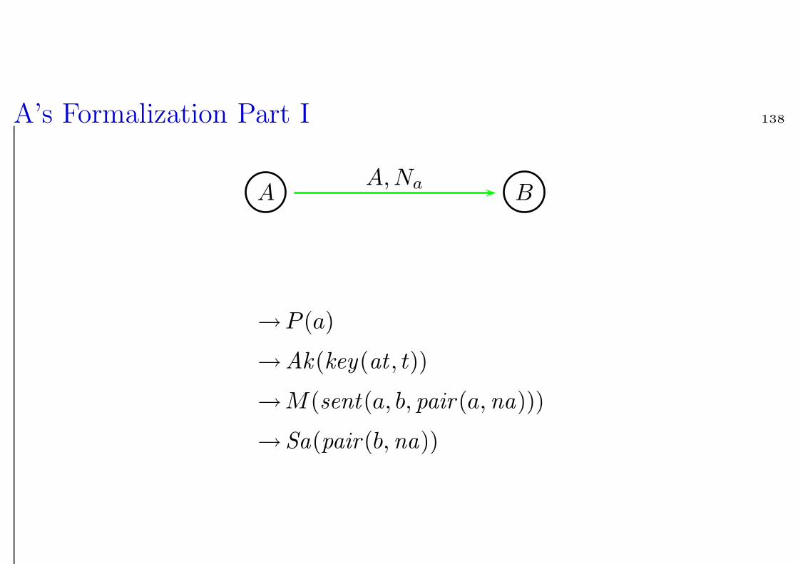
A’s Formalization Part I 138
AA,Na B
→P (a)
→Ak(key(at , t))
→M(sent(a, b, pair (a,na)))
→Sa(pair(b,na))
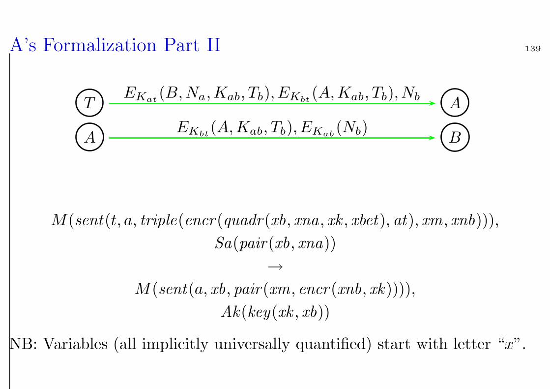
A’s Formalization Part II 139
TEKat
(B,Na,Kab, Tb), EKbt(A,Kab, Tb), Nb A
AEKbt
(A,Kab, Tb), EKab(Nb) B
M(sent(t, a, triple(encr(quadr(xb, xna, xk , xbet), at), xm, xnb))),
Sa(pair(xb, xna))
→
M(sent(a, xb, pair(xm, encr (xnb, xk)))),
Ak(key(xk , xb))
NB: Variables (all implicitly universally quantified) start with letter “x”.
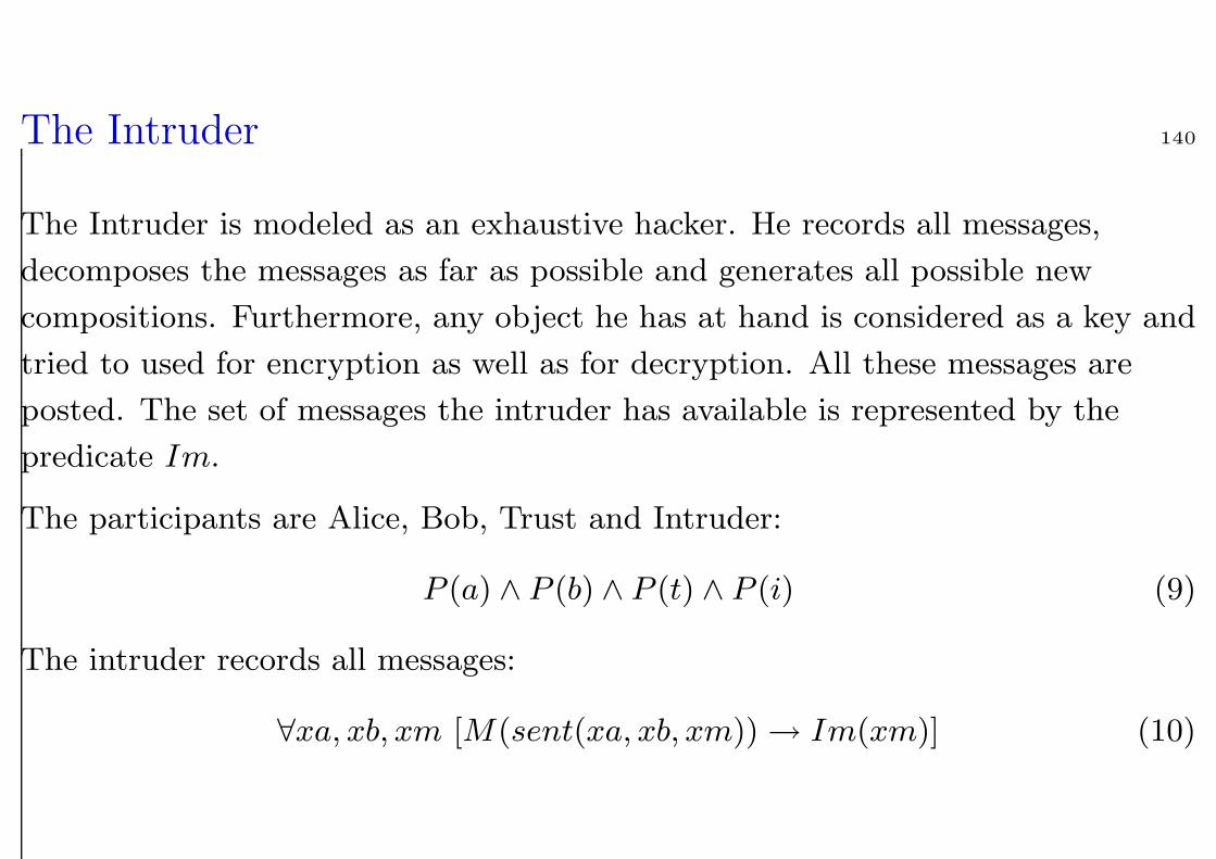
The Intruder 140
The Intruder is modeled as an exhaustive hacker. He records all messages,
decomposes the messages as far as possible and generates all possible new
compositions. Furthermore, any object he has at hand is considered as a key and
tried to used for encryption as well as for decryption. All these messages are
posted. The set of messages the intruder has available is represented by the
predicate Im.
The participants are Alice, Bob, Trust and Intruder:
P (a) ∧ P (b) ∧ P (t) ∧ P (i) (9)
The intruder records all messages:
∀xa, xb, xm [M(sent(xa, xb, xm)) → Im(xm)] (10)
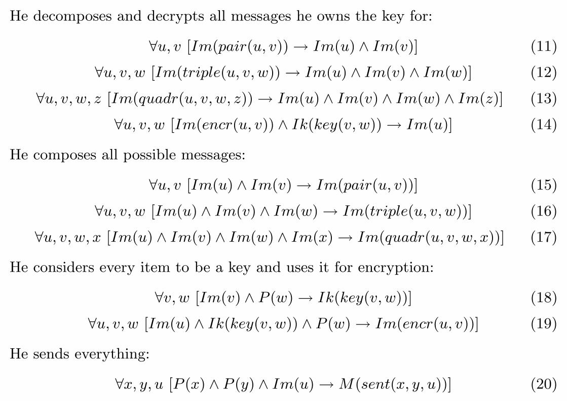
He decomposes and decrypts all messages he owns the key for:
∀u, v [Im(pair(u, v)) → Im(u) ∧ Im(v)] (11)
∀u, v, w [Im(triple(u, v, w)) → Im(u) ∧ Im(v) ∧ Im(w)] (12)
∀u, v, w, z [Im(quadr(u, v, w, z)) → Im(u) ∧ Im(v) ∧ Im(w) ∧ Im(z)] (13)
∀u, v, w [Im(encr(u, v)) ∧ Ik(key(v, w)) → Im(u)] (14)
He composes all possible messages:
∀u, v [Im(u) ∧ Im(v) → Im(pair(u, v))] (15)
∀u, v, w [Im(u) ∧ Im(v) ∧ Im(w) → Im(triple(u, v, w))] (16)
∀u, v, w, x [Im(u) ∧ Im(v) ∧ Im(w) ∧ Im(x) → Im(quadr(u, v, w, x))] (17)
He considers every item to be a key and uses it for encryption:
∀v, w [Im(v) ∧ P (w) → Ik(key(v, w))] (18)
∀u, v, w [Im(u) ∧ Ik(key(v, w)) ∧ P (w) → Im(encr(u, v))] (19)
He sends everything:
∀x, y, u [P (x) ∧ P (y) ∧ Im(u) → M(sent(x, y, u))] (20)
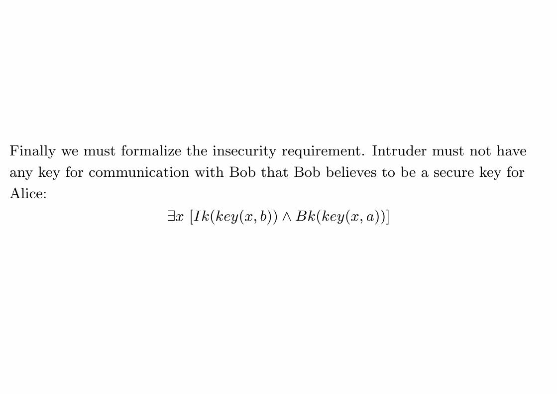
Finally we must formalize the insecurity requirement. Intruder must not have
any key for communication with Bob that Bob believes to be a secure key for
Alice:
∃x [Ik(key(x, b)) ∧ Bk(key(x, a))]
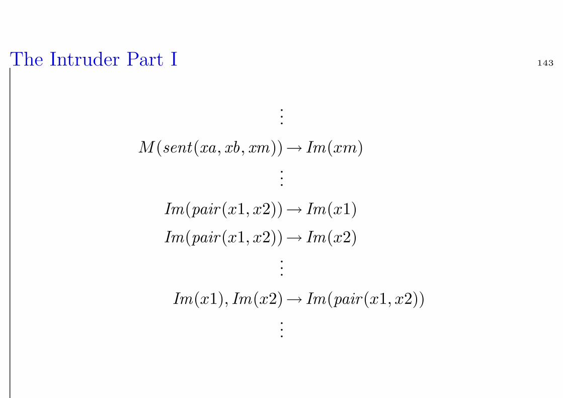
The Intruder Part I 143
...
M(sent(xa, xb, xm))→ Im(xm)...
Im(pair(x1, x2))→ Im(x1)
Im(pair(x1, x2))→ Im(x2)...
Im(x1), Im(x2)→ Im(pair(x1, x2))...
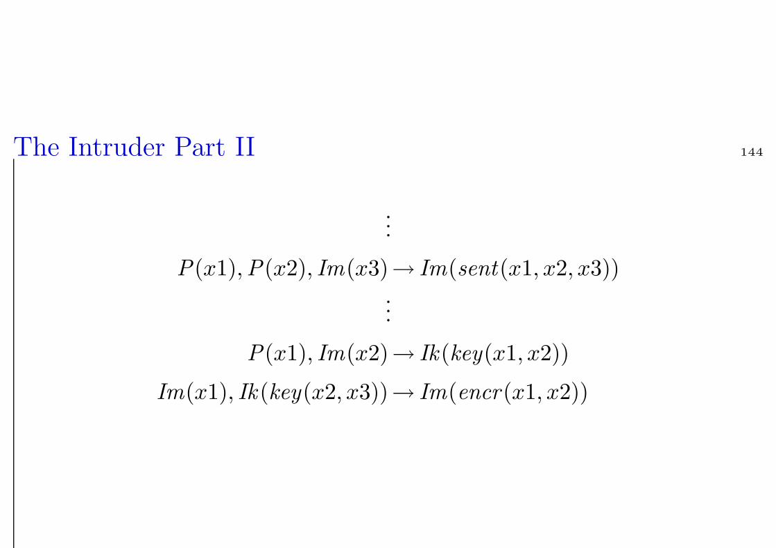
The Intruder Part II 144
...
P(x1),P(x2), Im(x3)→ Im(sent(x1, x2, x3))...
P(x1), Im(x2)→ Ik(key(x1, x2))
Im(x1), Ik (key(x2, x3))→ Im(encr(x1, x2))
SPASS solves the problem 145
Now the protocol formulae (1)-(8) together with the intruder formulae (9)-(20)
and the insecurity formula above can be given to SPASS. Then SPASS
automatically proves that this formula holds and that the problematic key is the
nonce Na. The protocol can be repaired by putting type checks on the keys,
such that keys can no longer be confused with nonces. This can be added to the
SPASS first-order logic formalization. Then SPASS disproves the insecurity
formula above. This capability is currently unique to SPASS. Although some
other provers might be able to prove that the insecurity formula holds in the
formalization without type checks, we are currently not aware of any prover that
can disprove the insecurity formula in the formalization with type checking.
Further details can be found in [2], below. The experiment is available in full
detail from the SPASS home page in the download area.
References:
[1] Neuman, B. C. and Stubblebine, S. G., 1993, A note on the use of
timestamps as nonces, ACM SIGOPS, Operating Systems Review, 27(2), 10-14.
[2] Weidenbach, C., 1999, Towards an automatic analysis of security protocols in
first-order logic, in 16th International Conference on Automated Deduction,
CADE-16, Vol. 1632 of LNAI, Springer, pp. 378-382.
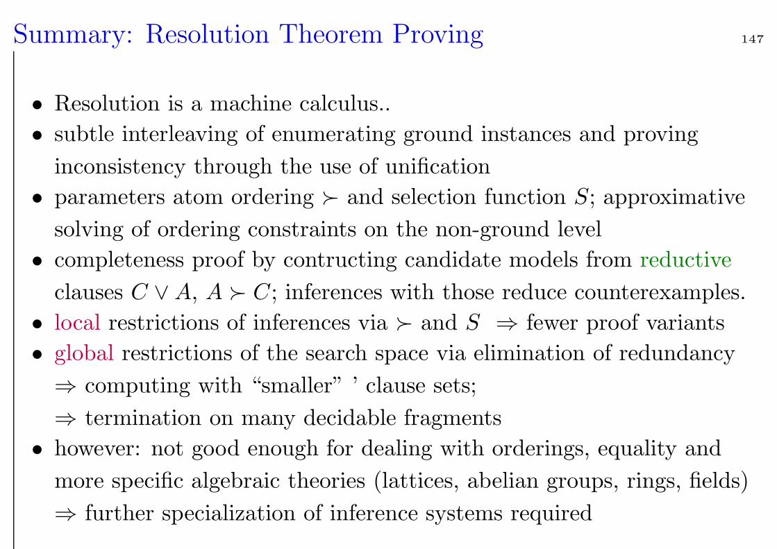
Summary: Resolution Theorem Proving 147
• Resolution is a machine calculus..
• subtle interleaving of enumerating ground instances and proving
inconsistency through the use of unification
• parameters atom ordering and selection function S; approximative
solving of ordering constraints on the non-ground level
• completeness proof by contructing candidate models from reductive
clauses C ∨A, A C; inferences with those reduce counterexamples.
• local restrictions of inferences via and S ⇒ fewer proof variants
• global restrictions of the search space via elimination of redundancy
⇒ computing with “smaller” ’ clause sets;
⇒ termination on many decidable fragments
• however: not good enough for dealing with orderings, equality and
more specific algebraic theories (lattices, abelian groups, rings, fields)
⇒ further specialization of inference systems required
1.11 Semantic Tableaux 148
analytic: inferences according to the logical content of the symbols
goal oriented: inferences operate directly on the goal to be proved
global: some inferences affect the entire proof state (set of formulas)
Literature: Fitting book, chapt. 3, 6, 7.
R.M. Smullyan: First-Order Logic, Dover Publ., New York, 1968,
revised 1995.
Like resolution, semantic tableaux were developed in the sixties, by R.M.
Smullyan,a on the basis of work by Gentzen in the 30ies and of Beth in the
50ies.aAccording to Fitting, semantic tableaux were first proposed by the Polish scientist
Z. Lis in a paper in Studia Logica 10, 1960 that was only recently rediscovered.
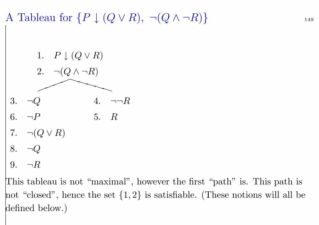
A Tableau for P ↓ (Q ∨R), ¬(Q ∧ ¬R) 149
3. ¬Q
6. ¬P
7. ¬(Q ∨R)
8. ¬Q
9. ¬R
4. ¬¬R
5. R
!!
!!
PP
PP
P
1. P ↓ (Q ∨R)
2. ¬(Q ∧ ¬R)
This tableau is not “maximal”, however the first “path” is. This path is
not “closed”, hence the set 1, 2 is satisfiable. (These notions will all be
defined below.)
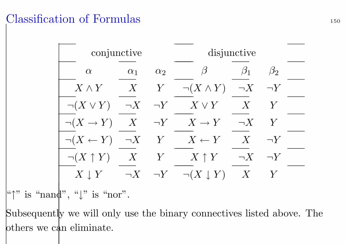
Classification of Formulas 150
conjunctive disjunctive
α α1 α2 β β1 β2
X ∧ Y X Y ¬(X ∧ Y ) ¬X ¬Y
¬(X ∨ Y ) ¬X ¬Y X ∨ Y X Y
¬(X → Y ) X ¬Y X → Y ¬X Y
¬(X ← Y ) ¬X Y X ← Y X ¬Y
¬(X ↑ Y ) X Y X ↑ Y ¬X ¬Y
X ↓ Y ¬X ¬Y ¬(X ↓ Y ) X Y
“↑” is “nand”, “↓” is “nor”.
Subsequently we will only use the binary connectives listed above. The
others we can eliminate.
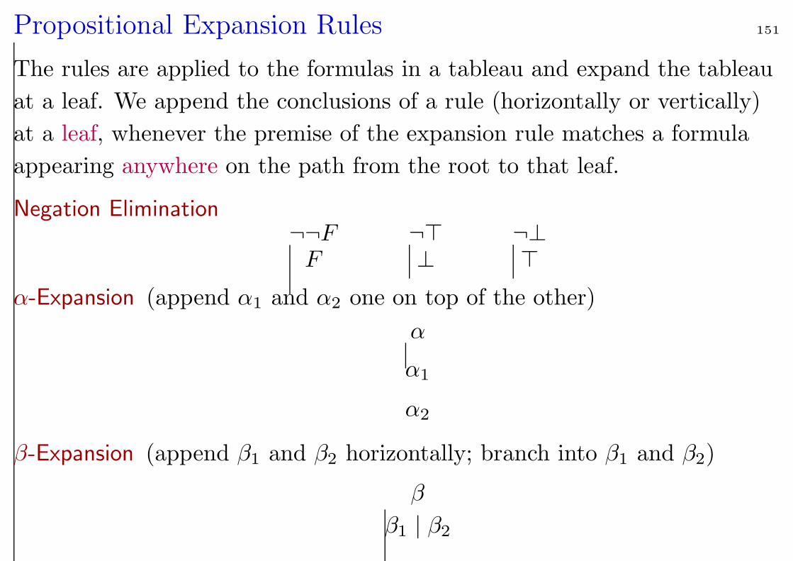
Propositional Expansion Rules 151
The rules are applied to the formulas in a tableau and expand the tableau
at a leaf. We append the conclusions of a rule (horizontally or vertically)
at a leaf, whenever the premise of the expansion rule matches a formula
appearing anywhere on the path from the root to that leaf.
Negation Elimination¬¬F
F¬>⊥
¬⊥>
α-Expansion (append α1 and α2 one on top of the other)
α
α1
α2
β-Expansion (append β1 and β2 horizontally; branch into β1 and β2)
β
β1 | β2
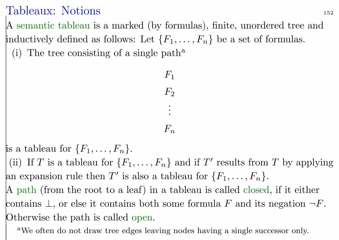
Tableaux: Notions 152
A semantic tableau is a marked (by formulas), finite, unordered tree and
inductively defined as follows: Let F1, . . . , Fn be a set of formulas.
(i) The tree consisting of a single patha
F1
F2
...
Fn
is a tableau for F1, . . . , Fn.
(ii) If T is a tableau for F1, . . . , Fn and if T ′ results from T by applying
an expansion rule then T ′ is also a tableau for F1, . . . , Fn.
A path (from the root to a leaf) in a tableau is called closed, if it either
contains ⊥, or else it contains both some formula F and its negation ¬F .
Otherwise the path is called open.aWe often do not draw tree edges leaving nodes having a single successor only.
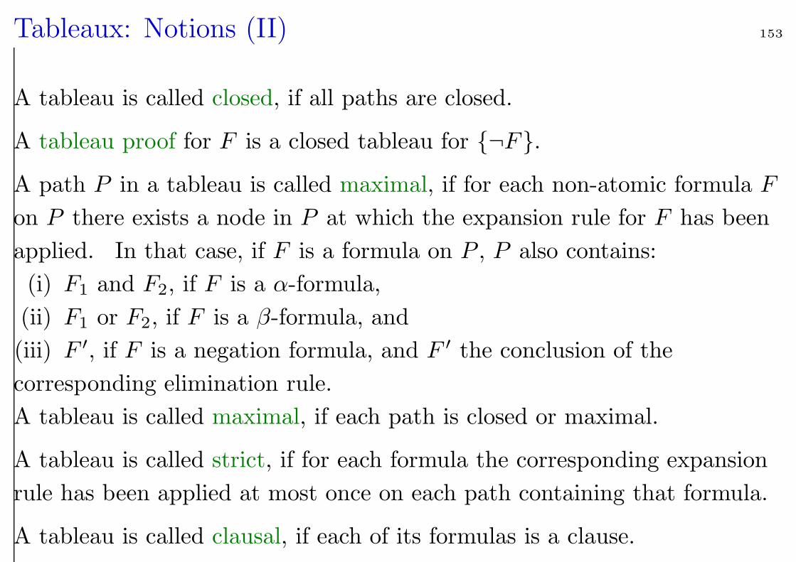
Tableaux: Notions (II) 153
A tableau is called closed, if all paths are closed.
A tableau proof for F is a closed tableau for ¬F.
A path P in a tableau is called maximal, if for each non-atomic formula F
on P there exists a node in P at which the expansion rule for F has been
applied. In that case, if F is a formula on P , P also contains:
(i) F1 and F2, if F is a α-formula,
(ii) F1 or F2, if F is a β-formula, and
(iii) F ′, if F is a negation formula, and F ′ the conclusion of the
corresponding elimination rule.
A tableau is called maximal, if each path is closed or maximal.
A tableau is called strict, if for each formula the corresponding expansion
rule has been applied at most once on each path containing that formula.
A tableau is called clausal, if each of its formulas is a clause.
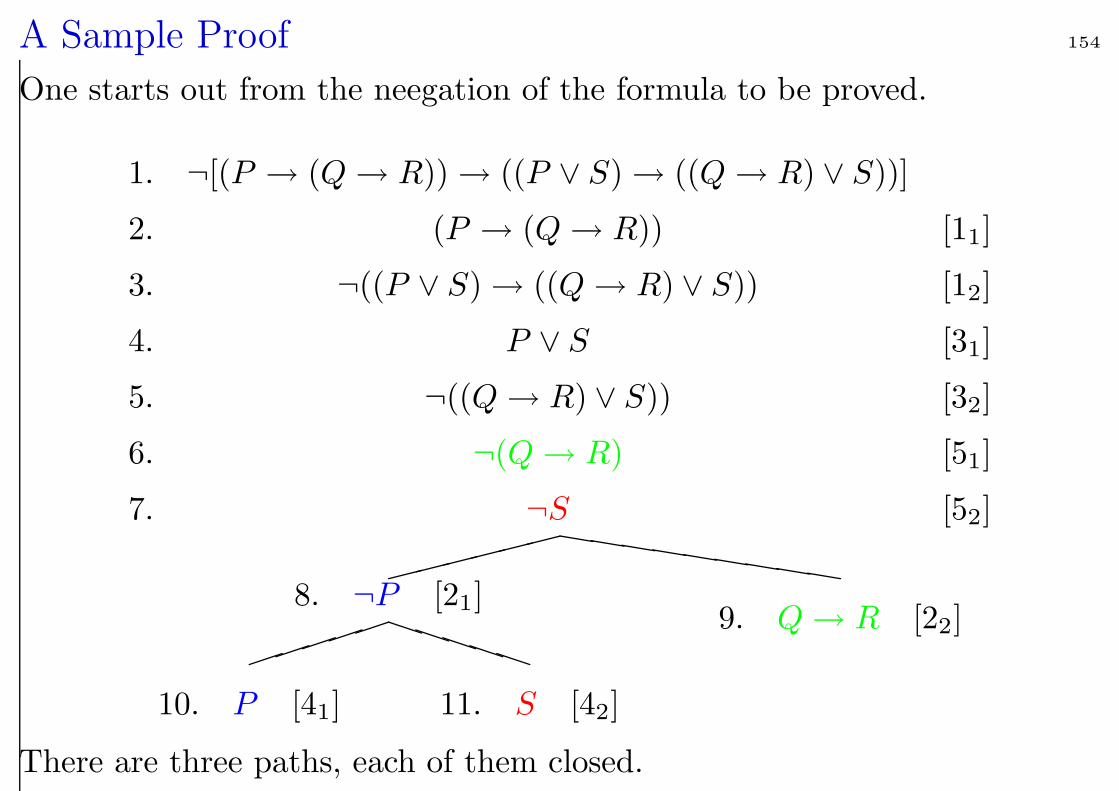
A Sample Proof 154
One starts out from the neegation of the formula to be proved.
10. P [41] 11. S [42]
PP
PP
P
8. ¬P [21]9. Q→ R [22]
hhhhhhhhh
1. ¬[(P → (Q→ R))→ ((P ∨ S)→ ((Q→ R) ∨ S))]
2. (P → (Q→ R)) [11]
3. ¬((P ∨ S)→ ((Q→ R) ∨ S)) [12]
4. P ∨ S [31]
5. ¬((Q→ R) ∨ S)) [32]
6. ¬(Q→ R) [51]
7. ¬S [52]
There are three paths, each of them closed.
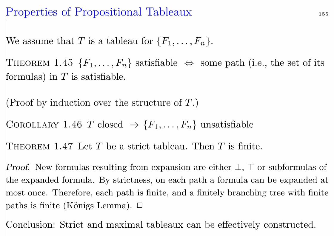
Properties of Propositional Tableaux 155
We assume that T is a tableau for F1, . . . , Fn.
Theorem 1.45 F1, . . . , Fn satisfiable ⇔ some path (i.e., the set of its
formulas) in T is satisfiable.
(Proof by induction over the structure of T .)
Corollary 1.46 T closed ⇒ F1, . . . , Fn unsatisfiable
Theorem 1.47 Let T be a strict tableau. Then T is finite.
Proof. New formulas resulting from expansion are either ⊥, > or subformulas of
the expanded formula. By strictness, on each path a formula can be expanded at
most once. Therefore, each path is finite, and a finitely branching tree with finite
paths is finite (Konigs Lemma). 2
Conclusion: Strict and maximal tableaux can be effectively constructed.
Refutational Completeness 156
Theorem 1.48 Let P be a maximal, open path in a tableau. Then set of
formulas on P is satisfiable.
Proof. [for the case of a clausal tableau] Let N be the set of formulas on P . As
P is open, ⊥ is not in N . Let C ∨ A and D ∨ ¬A be two resolvable clauses in N .
One of the two sublauses C or D, C say, is not empty, as otherwise P would be
closed. Since P is maximal, in P the β-rule was applied on C ∨ A. Therefore, P
(and N) contains a proper subclause of C ∨ A, and hence C ∨ A is redundant in
N . By the same reasoning, if N contains a clause that can be factored, that
clause must be redundant in N . In other words, N is saturated up to redundancy
wrt. Res(olution). Now apply Theorem 1.20 to prove satisfiability of N . 2
Theorem 1.49 F1, . . . , Fn satisfiable ⇔ there exists no closed strict
tableau for F1, . . . , Fn.
Proof. One direction is clear by Theorem 1.45. For the reverse direction, let T
be a strict, maximal tableau for F1, . . . , Fn and let P be an open path in T .
By the previous Theorem the set of formulas on P , and hence by Theorem 1.45
the set F1, . . . , Fn, is satisfiable. 2
Consequences 157
The validity of a propositional formula F can be established by
constructing a strict, maximal tableau for ¬F:
• T closed ⇔ F valid.
• It suffices to test complementarity of paths wrt. atomic formulas (cf.
reasoning in the proof of Theorem 1.48).
• Which of the potentially many strict, maximal tableaux one computes
does not matter. In other words, tableau expansion rules can be
applied don’t-care non-deterministically (“proof confluence”).
• The expansion strategy, however, can have a dramatic impact on
tableau size.
• Since it is sufficient to saturate paths wrt. ordered resolution (up to
redundancy), tableau expansion rules can be even more restricted, in
particular by certain ordering constraints.
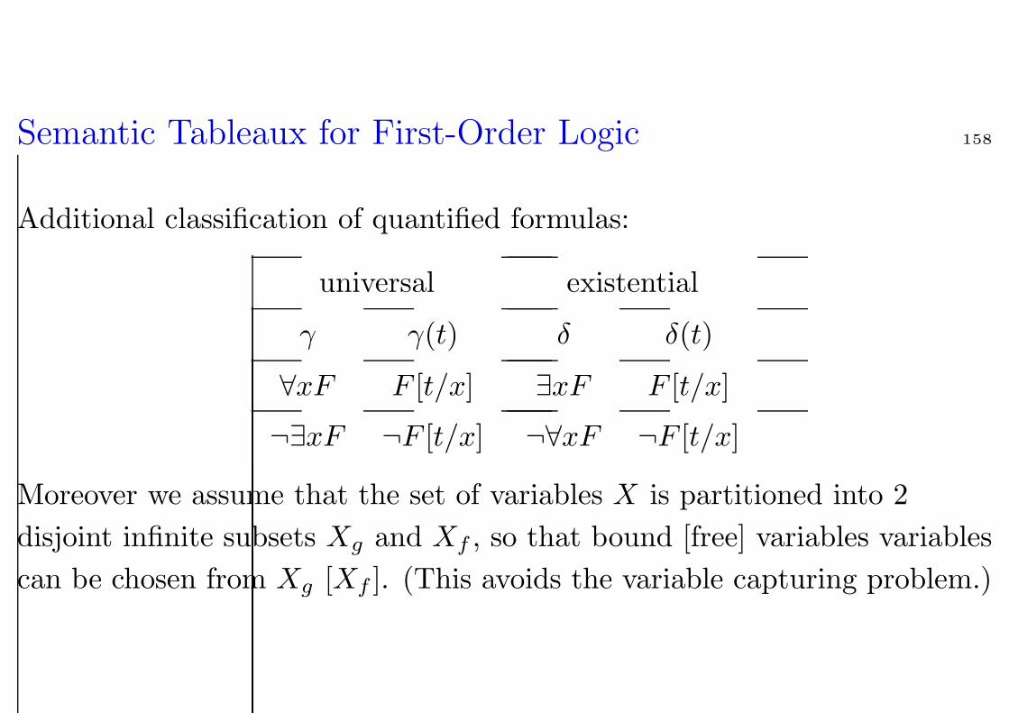
Semantic Tableaux for First-Order Logic 158
Additional classification of quantified formulas:
universal existential
γ γ(t) δ δ(t)
∀xF F [t/x] ∃xF F [t/x]
¬∃xF ¬F [t/x] ¬∀xF ¬F [t/x]
Moreover we assume that the set of variables X is partitioned into 2
disjoint infinite subsets Xg and Xf , so that bound [free] variables variables
can be chosen from Xg [Xf ]. (This avoids the variable capturing problem.)
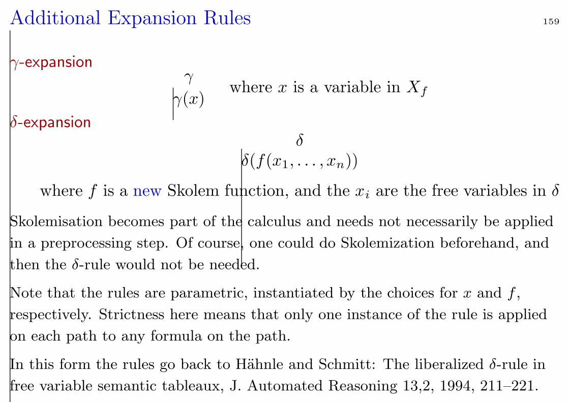
Additional Expansion Rules 159
γ-expansionγ
γ(x)where x is a variable in Xf
δ-expansionδ
δ(f(x1, . . . , xn))
where f is a new Skolem function, and the xi are the free variables in δ
Skolemisation becomes part of the calculus and needs not necessarily be applied
in a preprocessing step. Of course, one could do Skolemization beforehand, and
then the δ-rule would not be needed.
Note that the rules are parametric, instantiated by the choices for x and f ,
respectively. Strictness here means that only one instance of the rule is applied
on each path to any formula on the path.
In this form the rules go back to Hahnle and Schmitt: The liberalized δ-rule in
free variable semantic tableaux, J. Automated Reasoning 13,2, 1994, 211–221.

Definition: Free-Variable Tableau 160
Let F1, . . . , Fn be a set of closed formulas.
(i) The tree consisting of the single path
F1
...
Fn
is a tableau for F1, . . . , Fn.
(ii) If T is a tableau for F1, . . . , Fn and if T ′ results by applying an
expansion rule to T , then T ′ is also a tableau for F1, . . . , Fn.
(iii) If T is a tableau for F1, . . . , Fn and if σ is a substitution, then Tσ is
also a tableau for F1, . . . , Fn.
The substitution rule (iii) may, potentially, modify all the formulas of a tableau.
This feature is what is makes the tableau method a global proof method.
(Resolution, by comparison, is a local method.)
Of one took (iii) literally, by repeated application of γ-rule one can enumerate all
substitution instances of the universally quantified formulas. That would be a
major drawback compared with resolution. Fortunately, we can improve on this.
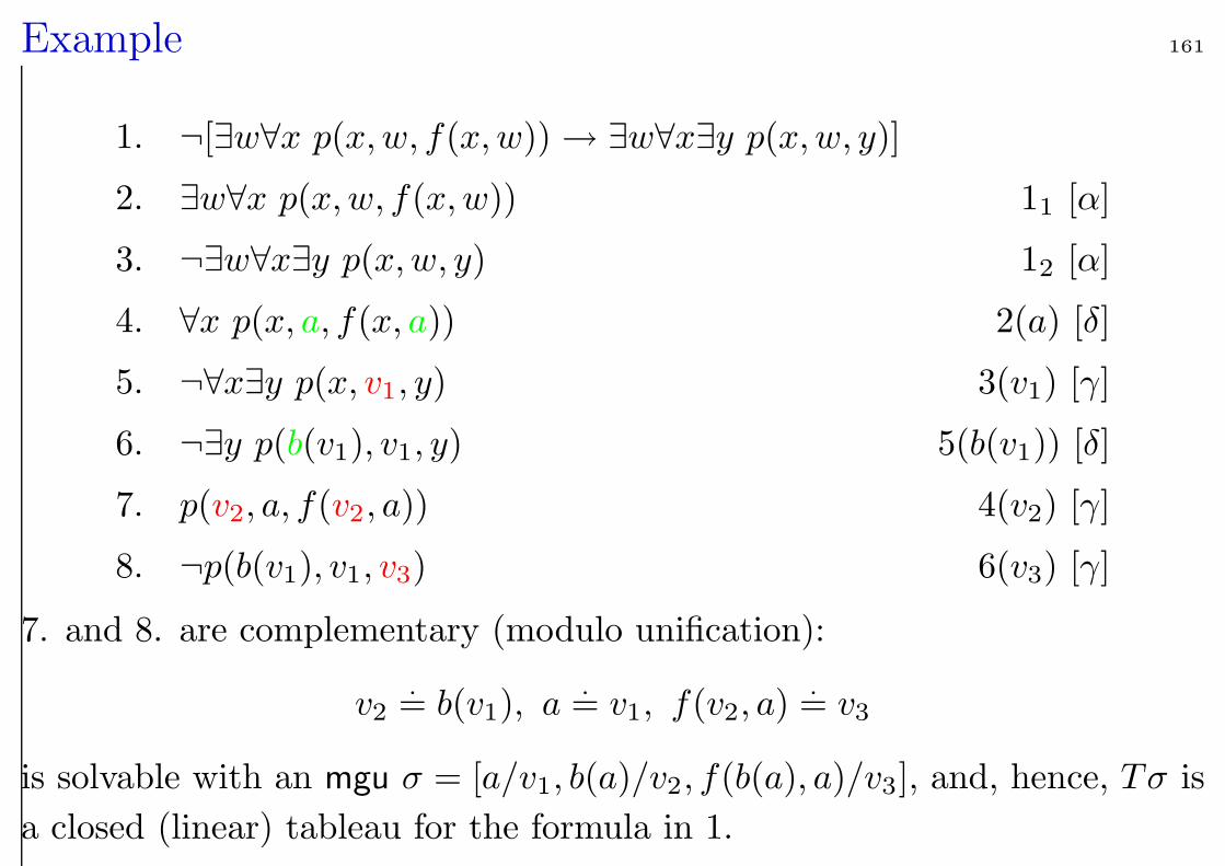
Example 161
1. ¬[∃w∀x p(x,w, f(x,w))→ ∃w∀x∃y p(x,w, y)]
2. ∃w∀x p(x,w, f(x,w)) 11 [α]
3. ¬∃w∀x∃y p(x,w, y) 12 [α]
4. ∀x p(x, a, f(x, a)) 2(a) [δ]
5. ¬∀x∃y p(x, v1, y) 3(v1) [γ]
6. ¬∃y p(b(v1), v1, y) 5(b(v1)) [δ]
7. p(v2, a, f(v2, a)) 4(v2) [γ]
8. ¬p(b(v1), v1, v3) 6(v3) [γ]
7. and 8. are complementary (modulo unification):
v2.= b(v1), a
.= v1, f(v2, a)
.= v3
is solvable with an mgu σ = [a/v1, b(a)/v2, f(b(a), a)/v3], and, hence, Tσ is
a closed (linear) tableau for the formula in 1.
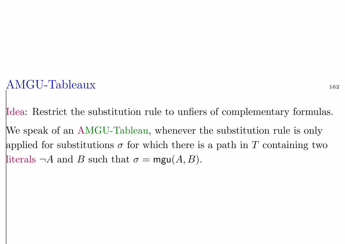
AMGU-Tableaux 162
Idea: Restrict the substitution rule to unfiers of complementary formulas.
We speak of an AMGU-Tableau, whenever the substitution rule is only
applied for substitutions σ for which there is a path in T containing two
literals ¬A and B such that σ = mgu(A,B).
Correctness 163
Given an signature Σ, by Σsko we denote the result of adding infinitely
many new Skolem function symbols which we may use in the δ-rule.
Let A be a Σsko-interpretation, T a Tableau, and β a variable assignment
over A. T is called (A, β)-valid, if there is a path Pβ in T such that
A, β |= F , for each formula F on Pβ. T is called satisfiable if there exists a
structure A such that for each assignment β the tableau T is (A, β)-valid.
(This implies that we may choose Pβ depending on β.)
Let Fi be closed Σ-formulas.
Theorem 1.50 Let T be a tableau for F1, . . . , Fn.
F1, . . . , Fn is satisfiable ⇔ T is satisfiable.
(Proof of “ ⇒ ” by induction over the depth of T . For δ one needs to reuse
the ideas for proving that Skolemization preserves [un-]satisfiability.)
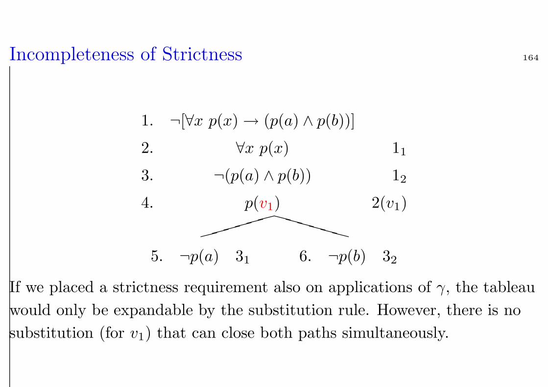
Incompleteness of Strictness 164
5. ¬p(a) 31 6. ¬p(b) 32
XXXXXX
1. ¬[∀x p(x)→ (p(a) ∧ p(b))]
2. ∀x p(x) 11
3. ¬(p(a) ∧ p(b)) 12
4. p(v1) 2(v1)
If we placed a strictness requirement also on applications of γ, the tableau
would only be expandable by the substitution rule. However, there is no
substitution (for v1) that can close both paths simultaneously.
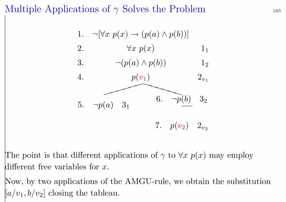
Multiple Applications of γ Solves the Problem 165
5. ¬p(a) 31
7. p(v2) 2v2
6. ¬p(b) 32
XXXXXX
1. ¬[∀x p(x)→ (p(a) ∧ p(b))]
2. ∀x p(x) 11
3. ¬(p(a) ∧ p(b)) 12
4. p(v1) 2v1
The point is that different applications of γ to ∀x p(x) may employ
different free variables for x.
Now, by two applications of the AMGU-rule, we obtain the substitution
[a/v1, b/v2] closing the tableau.
How Often Do we Have to Apply γ? 166
Theorem 1.51 There is no recursive function f : FΣ × FΣ → N such that,
if the closed formula F is unsatisfiable, then there exists a closed tableau
for F where to all formulas ∀xG appearing in T the γ-rule is applied at
most f(F,∀xG) times on each path containing ∀xG.
Otherwise unsatisfiablility or, respectively, validity for first-order logic would be
decidable. In fact, one would be able to enumerate in finite time all tableaux
bounded in depth as indicated by f . In other words, free-variable tableaux are
not recursively bounded in their depth.
Again ∀ is treated like an infinite conjunction. By repeatedly applying γ,
together with the substitution rule, one is capable of enumerating all instances
F [t/x] vertically, that is, conjunctively, in each path containing ∀xF .
Refutational Completeness 167
Therefore strictness for γ should from now on mean that each instance of
γ (depending on the choice of the free variable) is applied at most once to
each γ-formula on any path.
Theorem 1.52 F1, . . . , Fn satisfiable ⇔ there exists no closed, strict
AMGU-Tableau for F1, . . . , Fn.
For the proof one defines a fair tableau expansion process converging
against an infinite tableau where on each path each γ-formula is expanded
into all its variants (modulo the choice of the free variable).
One may then again show that each path in that tableau is saturated (up
to redundancy) by resolution. This requires to apply the lifting lemma for
resolution in order to show completeness of the AMGU-restriction.
Semantic Tableaux vs. Resolution 168
• Both methods are machine methods on which todays provers are based
upon.
• tableaux: global, goal-oriented, “backward”
• resolution: local, “forward”
• Resolution can be combined with more powerful redundancy
elimination methods.
• Like resolution, the tableau method, in order to be useful in practice,
must be accompanied by refinements: lemma generation, ordering
restrictions, efficient term and proof data structures
• Because of its global nature redundancy elimination is more difficult
for the tableau method.
• Resolution can be refined to work well with equality and algebraic
structures; tableaux cannot (it seems).
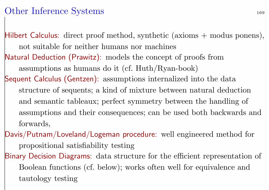
Other Inference Systems 169
Hilbert Calculus: direct proof method, synthetic (axioms + modus ponens),
not suitable for neither humans nor machines
Natural Deduction (Prawitz): models the concept of proofs from
assumptions as humans do it (cf. Huth/Ryan-book)
Sequent Calculus (Gentzen): assumptions internalized into the data
structure of sequents; a kind of mixture between natural deduction
and semantic tableaux; perfect symmetry between the handling of
assumptions and their consequences; can be used both backwards and
forwards,
Davis/Putnam/Loveland/Logeman procedure: well engineered method for
propositional satisfiability testing
Binary Decision Diagrams: data structure for the efficient representation of
Boolean functions (cf. below); works often well for equivalence and
tautology testing