mémoire présenté le€¦ · par dang diep nguyen: titre : reinsurance management in a big...
TRANSCRIPT

Mémoire présenté le :
pour l’obtention du Diplôme Universitaire d’actuariat de l’ISFA
et l’admission à l’Institut des Actuaires
Par : Dang Diep NGUYEN
Titre : Reinsurance management in a big insurance group: Risk-costing and optimization
Confidentialité : NON OUI (Durée : 1 an 2 ans)
Les signataires s’engagent à respecter la confidentialité indiquée ci-dessus.
Membres présents du jury de l’IA Signature Entreprise
B. Baltesar Nom : AXA Global Life
C. Pigeon Signature :
L. Eckert
Membres présents du jury de l’ISFA Directeur de mémoire en entreprise
D. Clot Nom : Hai Trung PHAM
Signature :
Invité
Nom :
Signature :
Autorisation de publication et de mise
en ligne sur un site de diffusion de
documents actuariels (après expiration
de l’éventuel délai de confidentialité)
Signature du responsable entreprise
Signature du candidat
Secrétariat :
Mme Christine DRIGUZZI
Bibliothèque :
Mme Patricia BARTOLO

Acknowledgement
Foremost, I would like to express my deepest gratitude to my tutor Mr. Hai Trung Pham for hisexcellent guidance and continuous support of my thesis. He was also tutor of my graduation intern-ship, which was a perfect opportunity to acquire practical knowledge in the world of business. Hismotivation, patience and his immense knowledge helped me eminently for the beginning of my careeras well as the accomplishment of this thesis.
Besides of my tutor, I also want to address my thanks to Risk Management team in AXA Global Lifeled by Mr Serge Da Marianna, with whom I worked during my graduation internship. Their hospitality,their patience and their advices made my first working experience an unforgettable memory.
My sincere thanks also go to my current team, Pricing team in AXA Global Life, especially Mrs.Frédérique Moy, Head of Pricing Department. Their experiences, their collaboration as well as thewarm working atmosphere give me the best environment to develop my professional competencies.I would like to present my special thanks to my colleague Mr. Samuel Weill, of whom expertisethroughout pricing field enlightened me in my works for this thesis.
I’m grateful to Frédéric Planchet my academic tutor. I appreciated his instruction and feedback whichwas essentially important for a good orientation and development of my thesis.
I would like to thank my mother, for giving birth to me at the first place and supporting me spirituallythroughout my life.
Finally and most importantly, I would like to thank my wife for her unlimited support, daily encour-agement, quiet patience and unwavering love.
1

Abstract
For decades, reinsurance has been one of the most important vehicles for risk management. It iscommon that nowadays, some big insurance groups have it own internal reinsurer entity in order toreduce the level of ceded profit externally in the one hand, and to benefit the diversification effect inthe other hand.
It exists two main missions for an internal reinsurer. The first one consists of the optimisation ofreinsurance program giving the specific needs of the local insurance entity. The second one consistsof a pricing model in order to challenge the external reinsurer’s prices.
The objectives of this report are in the one hand, to develop pricing models for non-proportionalreinsurance , and to assess the optimisation of reinsurance for an insurance company in the otherhand.
Regarding the first objective, the two most common non-proportional reinsurance were taken intoaccount in this report: Excess of loss per life and excess of loss per event Excess of loss perevent.With regard to the excess of loss per life, the first pricing model is a frequency-severity model whichpurely bases on the historical claim data and the size of portfolio. Our study was trying to introducethe truncated distributions in the calibration to see whether we can obtain better calibrationof atypical risk than the use of usual statistic distributions can. The calibration using truncateddistribution was largely applied in P&C reinsurance, it seems to be interesting to see its applicationin life reinsurance.In case of very limited claim data, the internal reinsurer could have alternative pricing model: usingthe Best Estimate incident rate risk and using the portfolio model point by Sum At Risk and by age.
With regard to the excess of loss per event, the report aims to continue the road of the past CATmodels in life insurance such as Strickler’s (1960) and Erland Ekheden’s (2008) by: extending the CATevents database - using terrorism database (GTD), simulating claim data using Sum At Risk modelpoint and adding geographical deterministic scenarios in the simulation. In particular, we would liketo test the application of other "fat tail" distributions than the traditional distribution for CAT claims:Generalized Pareto Distribution.
For the second objective, we will assume that the insurance company uses standard formula factors inits calculation of Solvency Capital Requirement. Then based on its specific needs in terms of volatilityand required capital, we try to determine the optimized reinsurance structure.
Key words: non-proportional reinsurance, excess of loss per life, excess of loss per event, truncateddistribution, Generalized Pareto Distribution, Solvency Capital Requirement, optimisation.
2

Résumé
Depuis des décennies, la réassurance est l’un des principaux outils de la gestion des risques. Il estfréquent que de nos jours, certains grands groupes d’assurance disposent d’un réassureur internequi aide d’une part à réduire le profit cédé extérieurement et d’autre part à bénéficier de l’effet dediversification.
Il existe deux missions principales pour un réassureur interne. La première consiste à optimiserle programme de réassurance de l’entité locale en répondant à ses besoins spécifiques. La secondeconsiste à établir un modèle de tarification afin de challenger les prix du réassureur externe.
Les objectifs de ce rapport sont d’une part d’élaborer des modèles de tarification pour la réassurancenon-proportionnelle et d’autre part de proposer les indicateurs d’optimisation de la réassurancepour une entité locale.
En ce qui concerne le premier objectif, les deux réassurances non-proportionelles les plus courants sontconsidérées: excédent de sinistre par tête et excédent de sinistre par événement.Pour la réassurance excédent de sinistre par tête, le premier modèle de tarification est un mod-èle de fréquence-sévérité qui s’appuie sur les données historiques de sinistres. Notre étude a tentéd’introduire les distributions tronqées dans la calibration pour voir si nous pouvons obtenir un meilleurqualité de fit du risque atypique que l’utilisation des distributions statistiques habituelles. La cali-bration utilisant les distributions tronquées ont été largement appliqué en réassurance on-vie. Ilsemble intéressant de voir son application dans la réassurance vie.Au cas où les données de sinistres sont très limitées, le réassureur pourrait utiliser un autre modèlede tarification: modèle de taux d’incident Best Estimate en utilisant le modèle point du portefeuillepar Somme At Risk et l’âge.
Pour la réassurance excédent de sinistre par événement, le rapport vise à poursuivre des modèles detarification du risque CAT en vie tels que Strickler (1960) et Erland Ekheden (2008) en élargissantla base de données CAT en utilisant la base pour les événements terrorists - GTD; en simulantles montants de sinistre à l’aide du modèle point par Sum At Risk et en ajoutant des scénariosdéterministes. En particulier, nous aimerions tester l’application d’autres distributions de la "queueépaisse" que la distribution traditionnelle pour la caribration du risque CAT - distribution Paretogénéralisée.
En ce qui concerne le deuxième objectif, nous supposerons que la compagnie d’assurance utilise lesformules standards dans son calcul du capital de solvabilité requis . En suite, en fonction de ses besoinsspécifiques en termes de volatilité ou de capital requis, nous tentons de déterminer la structure deréassurance optimisée.
Mots clés: réassurance non proportionnelle, excédent de sinistre par tête, excédent de sinistre par événe-ment, distribution tronquée, Pareto distribution généralisée, capital requis, réassurance optimisée.
3

Contents
1 Introduction to life reinsurance 71.1 Brief definition of life reinsurance . . . . . . . . . . . . . . . . . . . . . . . . . . . . . . 7
1.1.1 Definition . . . . . . . . . . . . . . . . . . . . . . . . . . . . . . . . . . . . . . . 71.1.2 Covered risks . . . . . . . . . . . . . . . . . . . . . . . . . . . . . . . . . . . . . 71.1.3 Contractual elements . . . . . . . . . . . . . . . . . . . . . . . . . . . . . . . . . 8
1.2 Traditional life reinsurance and structured life reinsurance . . . . . . . . . . . . . . . . 91.3 Focus on traditional life reinsurance . . . . . . . . . . . . . . . . . . . . . . . . . . . . 9
1.3.1 Different types of traditional life reinsurance . . . . . . . . . . . . . . . . . . . 91.3.1.1 Proportional reinsurance . . . . . . . . . . . . . . . . . . . . . . . . . 101.3.1.2 Non-proportional reinsurance . . . . . . . . . . . . . . . . . . . . . . . 14
1.3.2 Data available to Reinsurer . . . . . . . . . . . . . . . . . . . . . . . . . . . . . 171.3.2.1 Portfolio data . . . . . . . . . . . . . . . . . . . . . . . . . . . . . . . 171.3.2.2 Public catastrophes data . . . . . . . . . . . . . . . . . . . . . . . . . 19
1.3.3 The role of traditional reinsurance for a life insurer . . . . . . . . . . . . . . . . 221.4 Reinsurance in Solvency II context . . . . . . . . . . . . . . . . . . . . . . . . . . . . . 22
1.4.1 Reinsurance in calculation of solvency capital requirement . . . . . . . . . . . . 221.4.1.1 Reinsurance under Solvency I . . . . . . . . . . . . . . . . . . . . . . . 221.4.1.2 Reinsurance under Solvency II . . . . . . . . . . . . . . . . . . . . . . 23
2 Non-proportional reinsurance pricing models 242.1 XL per life . . . . . . . . . . . . . . . . . . . . . . . . . . . . . . . . . . . . . . . . . . 26
2.1.1 Some important definitions . . . . . . . . . . . . . . . . . . . . . . . . . . . . . 262.1.2 Pricing model . . . . . . . . . . . . . . . . . . . . . . . . . . . . . . . . . . . . . 27
2.1.2.1 Grand principle . . . . . . . . . . . . . . . . . . . . . . . . . . . . . . 272.1.2.2 Frequency-severity approach . . . . . . . . . . . . . . . . . . . . . . . 272.1.2.3 Burning Cost method approach . . . . . . . . . . . . . . . . . . . . . 402.1.2.4 Incident rate approach . . . . . . . . . . . . . . . . . . . . . . . . . . 432.1.2.5 Combined approach . . . . . . . . . . . . . . . . . . . . . . . . . . . . 44
2.1.3 Application of proposed pricing models . . . . . . . . . . . . . . . . . . . . . . 452.1.3.1 Data . . . . . . . . . . . . . . . . . . . . . . . . . . . . . . . . . . . . 452.1.3.2 Claim data descriptive statistics . . . . . . . . . . . . . . . . . . . . . 46
4

2.1.3.3 Pricing . . . . . . . . . . . . . . . . . . . . . . . . . . . . . . . . . . . 472.2 XL per event . . . . . . . . . . . . . . . . . . . . . . . . . . . . . . . . . . . . . . . . . 55
2.2.1 Risks covered by XL per event (CAT treaty) . . . . . . . . . . . . . . . . . . . 552.2.2 Treaty conditions . . . . . . . . . . . . . . . . . . . . . . . . . . . . . . . . . . . 552.2.3 Data analysis . . . . . . . . . . . . . . . . . . . . . . . . . . . . . . . . . . . . . 562.2.4 Pricing model . . . . . . . . . . . . . . . . . . . . . . . . . . . . . . . . . . . . . 59
2.2.4.1 Deterministic model . . . . . . . . . . . . . . . . . . . . . . . . . . . . 592.2.4.2 Model by simulation . . . . . . . . . . . . . . . . . . . . . . . . . . . . 612.2.4.3 Development of model by simulation . . . . . . . . . . . . . . . . . . . 652.2.4.4 Application . . . . . . . . . . . . . . . . . . . . . . . . . . . . . . . . . 66
3 Optimisation of reinsurance program 703.1 Retention and limit of XL per life . . . . . . . . . . . . . . . . . . . . . . . . . . . . . . 70
3.1.1 Different factors impacted by the level of retention . . . . . . . . . . . . . . . . 713.1.1.1 Expected profit and loss . . . . . . . . . . . . . . . . . . . . . . . . . . 713.1.1.2 Solvency capital requirement . . . . . . . . . . . . . . . . . . . . . . . 723.1.1.3 Volatility . . . . . . . . . . . . . . . . . . . . . . . . . . . . . . . . . . 723.1.1.4 Risk appetite . . . . . . . . . . . . . . . . . . . . . . . . . . . . . . . . 723.1.1.5 Level of services provided by reinsurer . . . . . . . . . . . . . . . . . . 72
3.1.2 Impact of reinsurance in solvency capital requirement . . . . . . . . . . . . . . 733.1.3 KPIs of cession . . . . . . . . . . . . . . . . . . . . . . . . . . . . . . . . . . . . 80
3.1.3.1 Cession without constraint . . . . . . . . . . . . . . . . . . . . . . . . 803.1.3.2 Cession with constraints . . . . . . . . . . . . . . . . . . . . . . . . . . 81
3.2 Retention and limit of XL CAT . . . . . . . . . . . . . . . . . . . . . . . . . . . . . . . 82
Appendix A Example: calculation of Cost of capital in Burning Cost pricing 84
5

List of Figures
1.1 Risk retrocession . . . . . . . . . . . . . . . . . . . . . . . . . . . . . . . . . . . . . . . 71.2 Quota-share reinsurance . . . . . . . . . . . . . . . . . . . . . . . . . . . . . . . . . . . 101.3 Surplus reinsurance . . . . . . . . . . . . . . . . . . . . . . . . . . . . . . . . . . . . . . 121.4 XL per Life reinsurance . . . . . . . . . . . . . . . . . . . . . . . . . . . . . . . . . . . 141.5 Stop-loss reinsurance . . . . . . . . . . . . . . . . . . . . . . . . . . . . . . . . . . . . . 171.6 Model point . . . . . . . . . . . . . . . . . . . . . . . . . . . . . . . . . . . . . . . . . . 181.7 Exclusion XL per event (CAT treaty) . . . . . . . . . . . . . . . . . . . . . . . . . . . 191.8 EMDAT database extraction . . . . . . . . . . . . . . . . . . . . . . . . . . . . . . . . 201.9 GTD database extration . . . . . . . . . . . . . . . . . . . . . . . . . . . . . . . . . . . 221.10 Impact of reinsurance under Solvency II . . . . . . . . . . . . . . . . . . . . . . . . . . 23
2.1 XL per life - List of claims higher than retention . . . . . . . . . . . . . . . . . . . . . 252.2 Example of truncated distribution - Logistic distribution . . . . . . . . . . . . . . . . . 382.3 Number of claims triangle . . . . . . . . . . . . . . . . . . . . . . . . . . . . . . . . . . 412.4 Amount of claim triangle . . . . . . . . . . . . . . . . . . . . . . . . . . . . . . . . . . 422.5 Model point for XL per Life pricing . . . . . . . . . . . . . . . . . . . . . . . . . . . . 432.6 Goodness of fit criteria . . . . . . . . . . . . . . . . . . . . . . . . . . . . . . . . . . . . 502.7 Truncated Weibull cumulative distribution function . . . . . . . . . . . . . . . . . . . . 512.8 Usual Weibull and lognormal cumulative distribution function . . . . . . . . . . . . . . 522.9 Incident approach . . . . . . . . . . . . . . . . . . . . . . . . . . . . . . . . . . . . . . . 532.10 Summary - results of XL per life reinsured risk-costing models . . . . . . . . . . . . . 542.11 Hill plot . . . . . . . . . . . . . . . . . . . . . . . . . . . . . . . . . . . . . . . . . . . . 672.12 Best fit distribution for the number of victims . . . . . . . . . . . . . . . . . . . . . . . 672.13 C.d.f of GPD vs other distributions . . . . . . . . . . . . . . . . . . . . . . . . . . . . . 68
3.1 Retention per life management . . . . . . . . . . . . . . . . . . . . . . . . . . . . . . . 713.2 Solvency Capital Requirement tree . . . . . . . . . . . . . . . . . . . . . . . . . . . . . 733.3 Cost of capital net of reinsurance . . . . . . . . . . . . . . . . . . . . . . . . . . . . . . 813.4 Cost of capital reduction after the reinsurance . . . . . . . . . . . . . . . . . . . . . . . 813.5 Standard deviation of net claim amount . . . . . . . . . . . . . . . . . . . . . . . . . . 823.6 Volatility reduction after reinsurance . . . . . . . . . . . . . . . . . . . . . . . . . . . . 82
6

Chapter 1
Introduction to life reinsurance
1.1 Brief definition of life reinsurance
1.1.1 Definition
Reinsurance can be defined as a coverage purchased by an insurer to cover all or a part of risksfrom insurance policies issued by this company. This buying action is called a "cession", the insur-ance company is called "ceding company". The Reinsurer can then also cede the risk or a part ofit to other Reinsurers. This action is called "retrocession" and the other Reinsurers are known as"retrocessionaires".
Figure 1.1: Risk retrocession
1.1.2 Covered risks
One or more categories of risks can be covered by a reinsurance contract. In particular, for lifeinsurance business:
• Mortality and morbidity
• Disability
• Medical expense
• Critical illness
• Longevity
• Others
7

In a reinsurance treaty, we have often a list of exclusion. For example: participating in a criminalact, suicide or self-inflicted injury, etc. In general, they are risks that are difficult to handle by thereinsurer.In addition, the "High Risk Occupation" (HRO) and the "High Risk Business" (HRB) are submittedas "Special Acceptances". The reinsurer could either decline or accept the risk with or without extra-loading.High Risk Business: Individual Policies of the kinds particularized in the reinsurance treaty. Forexample: Short-term travel accident policies.High Risk Occupation: The occupations of Original Insured considered to be of greater risk suchas: Professional sport-players, cabin crew and pilots of the airline companies, workers in mineralactivities.
1.1.3 Contractual elements
The contractual elements between the players mentioned in previous section are written in a legalagreement called: Reinsurance treaty. One can find following important technical notions in a lifereinsurance treaty:
Reinsurer expense: a sum calculated as a percentage of the Reinsurance Premium. It representsthe expenses issued from Reinsurer’s activities linked to the covered treaty.
Premium commission: The commission payable by Reinsurer to Reinsured for its administra-tive activities of original insurance policies.
Profit sharing commission: The amount of profit from Reinsurer to be shared with Reinsuredif the treaty makes profit for the Reinsurer.
Minimum Deposit Premium: The first and fixed amount payable by Reinsured to Reinsureras premium. The remaining amount will be calculated in function of claims amount during the year.
Sum at risk: under a Policy or for a given period of insurance, the difference between:the insuredbenefit or the present value of the benefits payable in the event of a Claim and the correspondingtechnical reserve, if any, at the date of the Claim. From now on, this term will be noted as "SAR".
Deductible: in respect of any Claim, the amount of Ultimate Net Loss retained by the Reinsuredfor its own account.
Limit: the maximum amount covered by the Reinsurance Agreement in respect of each CoveredLoss, in excess of the Deductible.
8

Annual Aggregate Limit: the maximum amount covered by the Reinsurance Agreement in onecovered year.
Special Acceptances: agreement by the Reinsurer to include risks as Covered risks where, un-less specifically agreed, Acceptances such risks would ordinarily not be accepted or would be excludedfrom cover or, if covered, would be subject to limitations.
Claim bordereau: The file sent by reinsured containing historical claim triggering the reinsur-ance treaty.
Premium bordereau: The file containing all information about reinsurance premium, especiallyusing for reinsurance per insured life.
1.2 Traditional life reinsurance and structured life reinsurance
We distinguish two main kinds of life reinsurance which are traditional reinsurance and struc-tured reinsurance. Traditional reinsurance can be defined as a vehicle of transfer of risks forexample: mortality, morbidity, disability and medical expense. The current thesis will only focus onthe traditional reinsurance.It’s also interesting to notice that in the more recent period, structured reinsurance by definition,is used as important tools for insurers to achieve some objectives, for example: to optimize thediversification of risks, to reduce the taxes, volume of reserve or cost of capital etc. When structuredreinsurance involves risk transfer, the risk transfer purpose is only secondary.
1.3 Focus on traditional life reinsurance
1.3.1 Different types of traditional life reinsurance
There are two main kinds of traditional reinsurance: proportional and non-proportional.In proportional basis, the reinsurance premium is indicated proportionally to the insurance premiumor to the ceded sum at risk of each insured. In contrast, in non-proportional basis, the reinsurancepremium is indicated globally for the total ceded portfolio.Technical notions: If the insurance portfolio contains n policies with the corresponding sum at risksXi,i=1,..,n and the corresponding insurance premiums: Pi,i=1,..,n.The reinsurance premium is noted as P re. If the reinsurance premiums are given per life, we noteP rei,i=1,..,n
9

1.3.1.1 Proportional reinsurance
The main types of proportional reinsurance in the market are: quota-share and surplus.a) Quota-share - QSReinsurer and insurer share the premium and the amount of claim in quota basis. The quota-shareratio, i.e. "cession rate" is noted q, then 1 -q would be called "retention rate". We have reinsurancepremium:
P re = q.n∑i=1
Pi
If there is a claim occurred for policy j, then, the amount of claim paid by Reinsurer called "claimrecovery" is equal to:
Cj = q.Xj and C =∑j
Cj
where C is total amount of claims during the covered period In the treaty wording, there would bea clause which limits the amount of sum at risk accepted by Reinsurer. This limit is often called"Underwriting limit". Above this level, the policies could be classed as "Special acceptances".The following graph shows an example of quota-share reinsurance with the ceded quota-share ratiobeing equal to 25%.
Figure 1.2: Quota-share reinsurance
The treaty could introduce a clause of profit sharing commission. Thus, the reinsurance result is thecombination of reinsurance premium and claim, expense and commission, and profit sharing, i.e:
10

Reins.re = Pre(1−RC)− C − PS.(Pre(1−RC − α)− C)
Where :
• Preins.re: Reinsurance result
• RC : Reinsurance premium commission
• C: Claims amount
• PS: Profit sharing ratio
• α: Reinsurer expense
b) Surplus per life - XPThe Surplus treaty is another form of proportional reinsurance but in practice, it introduces followingnotions as in non-proportional treaty:
• R: Retention
• L: Limit
The treaty Surplus is noted in this case: L XP R.The retention and limit are applied in per head or per policy level. A sum at risk Xi is assigned toeach insured or each policy. From the following calculation, the treaty defines the cession rate r foreach insured or each policy:
r = min( LXi,max(1− R
Xi, 0))
For mortality coverage with lump-sum payment in case of claim, the amount of claim is generallyfixed by the sum at risk Xi and the treaty reimbursement mechanism works exactly as XL per Lifenon-proportional treaty: reinsurer engages to pay any amount of claim exceeding the retention andlimited to the limit of the treaty, i.e. shown by following formulas:
Xrei = min(L,max(Xi −R, 0))
However, for disability coverage, the amount of claim sometimes depends on the level of disability andtherefore isn’t fixed at the sum at risk level. The cession rate is used in this case:
Xrei = Xi ∗ r
The graph below shows the part of Reinsurer and insurer in sum at risk for a Surplus reinsurance 5mXP 1m with mortality coverage:
11

Figure 1.3: Surplus reinsurance
As precised from the start, the reinsurance premium is calculated in proportional basis, per policy by2 kinds of basis:
• Quota-share basis:
Pre(i) = Xrei
Xi.Pi
Reinsurance premium is proportional to the original premium.
• Risk premium basis:Pre(i) = Xre
i .qxi
Reinsurer gives the specific rates applied to the ceded sum at risk which are generally differentfrom insurance premium rate.
In practice, risk premium basis is more frequently used than quota-share basis. The reinsurancepremium rate could be percentage of a reference table (e.g. regulation’s mortality table) or it couldbe a proper premium table calibrated by Reinsurer.An example of reinsurance premium table for policies with death benefit:
12
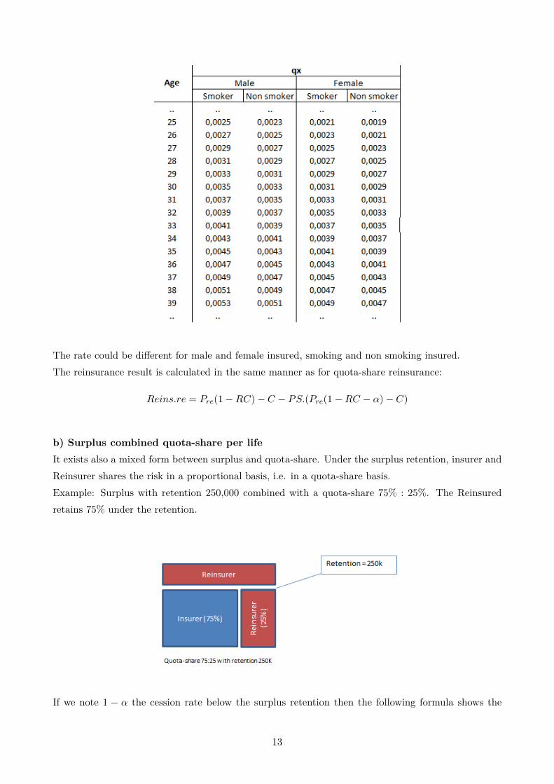
The rate could be different for male and female insured, smoking and non smoking insured.The reinsurance result is calculated in the same manner as for quota-share reinsurance:
Reins.re = Pre(1−RC)− C − PS.(Pre(1−RC − α)− C)
b) Surplus combined quota-share per lifeIt exists also a mixed form between surplus and quota-share. Under the surplus retention, insurer andReinsurer shares the risk in a proportional basis, i.e. in a quota-share basis.Example: Surplus with retention 250,000 combined with a quota-share 75% : 25%. The Reinsuredretains 75% under the retention.
If we note 1 − α the cession rate below the surplus retention then the following formula shows the
13
calculation of the reinsured sum at risk: Reinsured sum at risk:
Xrei = min(L,max(Xi −R, 0)) +min(Xi, R) ∗ (1− α)
Insurer’s retained sum at risk: Xi −Xrei
The reinsurance premium is normally defined in a risk premium basis (qx applied in ceded sum atrisk).The reinsurance result is calculated in the same manner as for proportionally surplus treaty.
1.3.1.2 Non-proportional reinsurance
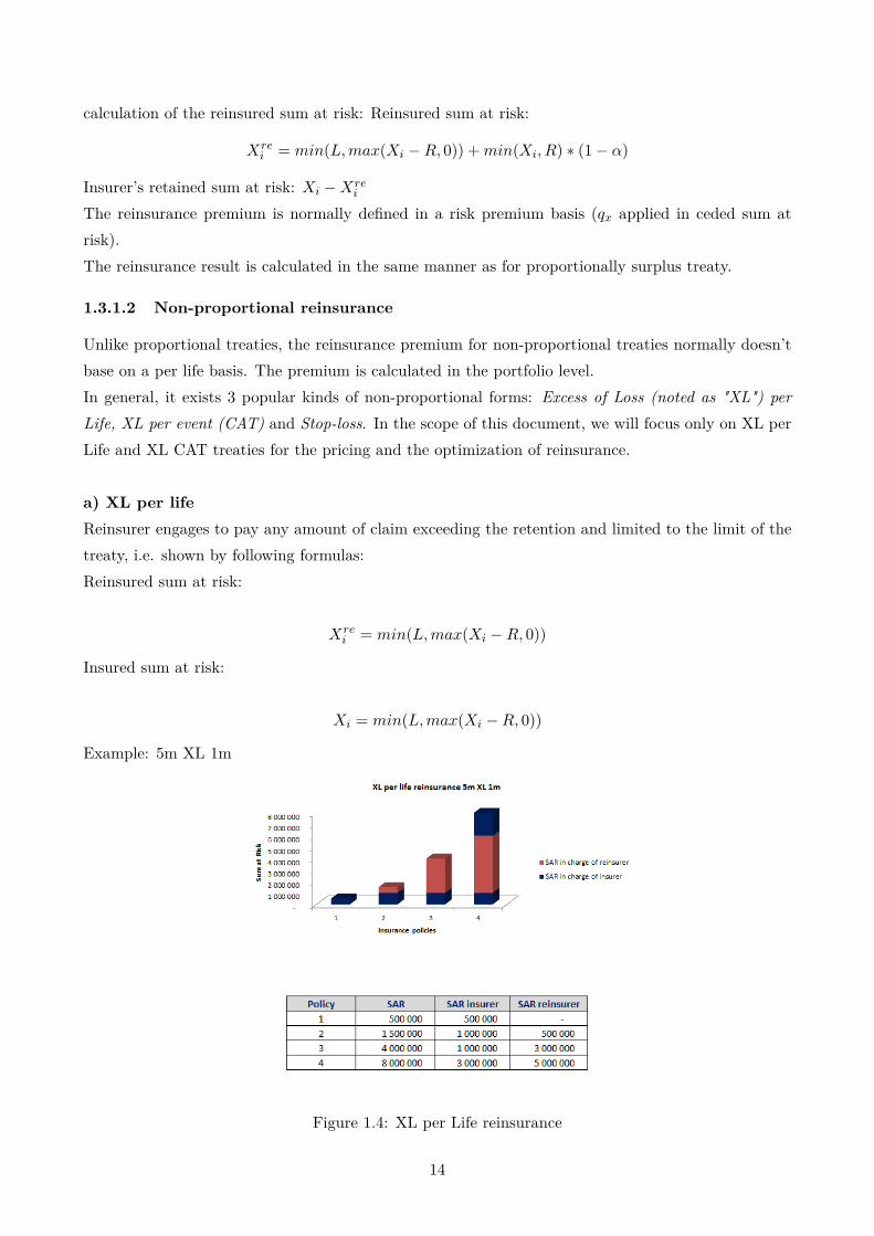
Unlike proportional treaties, the reinsurance premium for non-proportional treaties normally doesn’tbase on a per life basis. The premium is calculated in the portfolio level.In general, it exists 3 popular kinds of non-proportional forms: Excess of Loss (noted as "XL") perLife, XL per event (CAT) and Stop-loss. In the scope of this document, we will focus only on XL perLife and XL CAT treaties for the pricing and the optimization of reinsurance.
a) XL per lifeReinsurer engages to pay any amount of claim exceeding the retention and limited to the limit of thetreaty, i.e. shown by following formulas:Reinsured sum at risk:
Xrei = min(L,max(Xi −R, 0))
Insured sum at risk:
Xi = min(L,max(Xi −R, 0))
Example: 5m XL 1m
Figure 1.4: XL per Life reinsurance
14

In addition, it’s common for non-proportional treaties to have an AAL clause (aggregate annual loss)per year which is not likely to be included in proportional basis.
C = min(∑j
Cj , AAL)
Covered period:The covered period of XL per life treaty is normally one year (yearly renewable). This treaty coversall claims exceeding the retention of the treaty incurred during the covered period. The claim couldbe reported after the covered period (IBNyR - Chapter 2 - 2.1.1), or not enough reported during thecovered period (IBNeR - Chapter 2 - 2.1.1)Treaty conditions:
• R - Retention (deductible): The retention of the treaty. The claim amount has to exceed thislevel in order to activate the treaty.
• L - Limit (Capacity): The maximum obligation of Reinsurer per claim.
• n - Number of reinstatement: The maximum number of amounts of limit could be payable byreinsurer per year after the first used limit.
• AAL - Annual Aggregate Limit - The maximum total amount of reinsured claim payable byReinsurer per year: AAL = (n+1).L
Reinsurance premium: The reinsurance premium isn’t calculated by a proportional basis perinsured life. The reinsurance premium is given in form of rate of a premium basis. The premiumbasis could be EPI (Earned Premium Income) or ceded SAR. As the cover lasts during 1 year period,the rate is normally fixed at the beginning of the contract and re-adjusted at the end of the contractin function of the evolution of the premium basis. For example, if the premium basis stated in thetreaty is EPI, then at the time that the reinsurance treaty is issued (begining of year n), the Reinsurerpays normally an amount called "Minimum Deposit Premium" (MDP).
MDP = q.EPI01/01/n
At the end of the year, the Reinsurer and insurer readjust the reinsurance premium as following:
Pre = min(MDP, q.EPI01/01/n + EPI31/12/n
2 )
In general, the governance of reinsurance premium of XL per life treaty is much more simple than sur-plus reinsurance treaty as required no calculation per head. It’s often used when there is limited datain per life basis (in some countries, insurer can not obtain all per life information in group business).
b) XL per eventThe XL per event treaty (or also called in other words "CAT treaty") is placed by insurer after almost allother reinsurances such as per life and quota-share reinsurance in order to protect the portfolio against
15

extreme losses caused by natural catastrophic events or man-made catastrophic events (industrialhazard, terrorism attacks, etc.).Covered period:As XL per life treaty, XL per event treaty has also normally one year covered period (yearly renewable).This treaty covers also all claims exceeding the retention of the treaty incurred during the coveredperiod.Treaty conditions:
• R - Retention (deductible): The retention of the treaty. The claim amount per event has toexceed this level in order to activate the treaty.
• L - Limit (Capacity): The maximum obligation of Reinsurer per event.
• n - Number of reinstatement: The maximum number of amounts of limit could be payable byreinsurer per year after the first used limit.
• AAL - Annual Aggregate Limit - The maximum total amount of reinsured claim payable byReinsurer per year: AAL = (n+1).L
• Minimum number of victims: M - The minimum number of victims in the event in order toactivate the treaty.
c) XL Stop lossAs CAT treaty, Stop-loss is also a reinsurance after the placement of per life reinsurances.Stop-loss reinsurance will help to protect company result against the bad annual loss ratio due toeither number or size of claims.As already mentioned, a CAT cover will help the company be protected against a big catastrophicevent. However, the CAT cover generally excludes the risk of epidemic and pandemic. The stop-losscover, in complement to the CAT cover, can cover this risk and then can protect the final result of theinsurance company. Stop-loss reinsuance, therefore, not only protect the insurer against large claimsbut also large number of small claims during the year.
Example: Stop-loss reinsurance with retention 80% and capacity 120%. If the annual claims ratio(total claim/ total premium) exceeds 80%, the treaty will pay the exceeding part limited by thecapacity 120%.
16
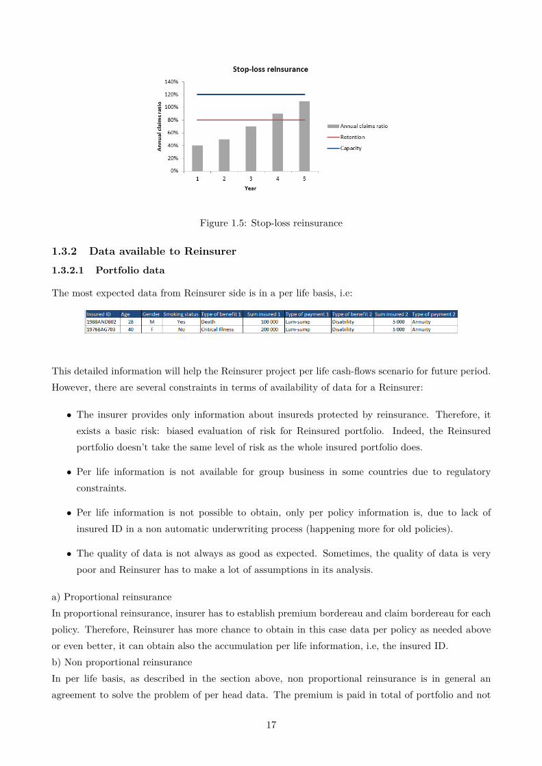
Figure 1.5: Stop-loss reinsurance
1.3.2 Data available to Reinsurer
1.3.2.1 Portfolio data
The most expected data from Reinsurer side is in a per life basis, i.e:
This detailed information will help the Reinsurer project per life cash-flows scenario for future period.However, there are several constraints in terms of availability of data for a Reinsurer:
• The insurer provides only information about insureds protected by reinsurance. Therefore, itexists a basic risk: biased evaluation of risk for Reinsured portfolio. Indeed, the Reinsuredportfolio doesn’t take the same level of risk as the whole insured portfolio does.
• Per life information is not available for group business in some countries due to regulatoryconstraints.
• Per life information is not possible to obtain, only per policy information is, due to lack ofinsured ID in a non automatic underwriting process (happening more for old policies).
• The quality of data is not always as good as expected. Sometimes, the quality of data is verypoor and Reinsurer has to make a lot of assumptions in its analysis.
a) Proportional reinsuranceIn proportional reinsurance, insurer has to establish premium bordereau and claim bordereau for eachpolicy. Therefore, Reinsurer has more chance to obtain in this case data per policy as needed aboveor even better, it can obtain also the accumulation per life information, i.e, the insured ID.b) Non proportional reinsuranceIn per life basis, as described in the section above, non proportional reinsurance is in general anagreement to solve the problem of per head data. The premium is paid in total of portfolio and not
17
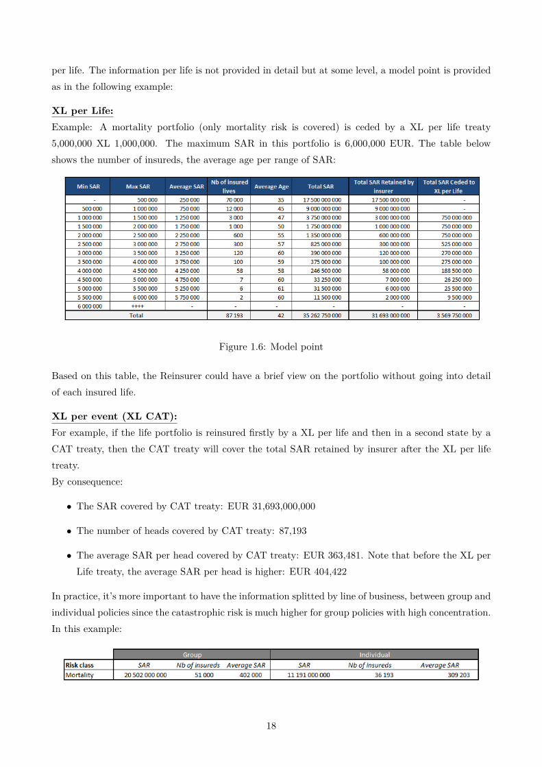
per life. The information per life is not provided in detail but at some level, a model point is providedas in the following example:
XL per Life:Example: A mortality portfolio (only mortality risk is covered) is ceded by a XL per life treaty5,000,000 XL 1,000,000. The maximum SAR in this portfolio is 6,000,000 EUR. The table belowshows the number of insureds, the average age per range of SAR:
Figure 1.6: Model point
Based on this table, the Reinsurer could have a brief view on the portfolio without going into detailof each insured life.
XL per event (XL CAT):For example, if the life portfolio is reinsured firstly by a XL per life and then in a second state by aCAT treaty, then the CAT treaty will cover the total SAR retained by insurer after the XL per lifetreaty.By consequence:
• The SAR covered by CAT treaty: EUR 31,693,000,000
• The number of heads covered by CAT treaty: 87,193
• The average SAR per head covered by CAT treaty: EUR 363,481. Note that before the XL perLife treaty, the average SAR per head is higher: EUR 404,422
In practice, it’s more important to have the information splitted by line of business, between group andindividual policies since the catastrophic risk is much higher for group policies with high concentration.In this example:
18

The risks covered by a reinsurance treaty should be relevant to the risks covered in the original policies(insurance policies), i.e., the CAT treaty shouldn’t cover the risks which are not covered by the originalpolicies. Therefore, the risks covered by insurance policies are provided as well.In this example:
Figure 1.7: Exclusion XL per event (CAT treaty)
In practice, the original policies always covers natural catastrophe risk and epidemic or pandemic risk.However, the epidemic and pandemic are not in the scope of this document. Also, the original policiesmay cover or not terrorism risk (bomb attacks, ambushes, etc), NBC (Nuclear, Biological, Chemical)and NBC terrorism risk. Political instability causes are normally covered except passive participationin war. High Risk Occupation is by default excluded in the reinsurance treaty. If Insurer wants tocover a group of high risk occupations (pilots, sport men, etc.), it has to request Reinsurer to put thegroup in a Special Acceptance.
1.3.2.2 Public catastrophes data
Natural CAT and man-made CAT except terrorism:For CAT treaties, in most cases, Reinsurer doesn’t possess enough claim data in its underlying portfo-lio. For the risk assessment, it has to use the data coming from general population in order to do thecalibration. A transformation step will be done in order to deduce the risk on the reinsured portfolio.
19

One of the most popular source of CAT data is EMDAT database (http://emdat.be/). An exampleof available information can be shown in the following table:
Figure 1.8: EMDAT database extraction
In order to understand better the database, we did some following descriptive statistics of the database.The using period is: 1900-2014.
Worst events in terms of number of deaths from 1970:
Statistics by type of disaster:
• Severity: 1900-2014
20
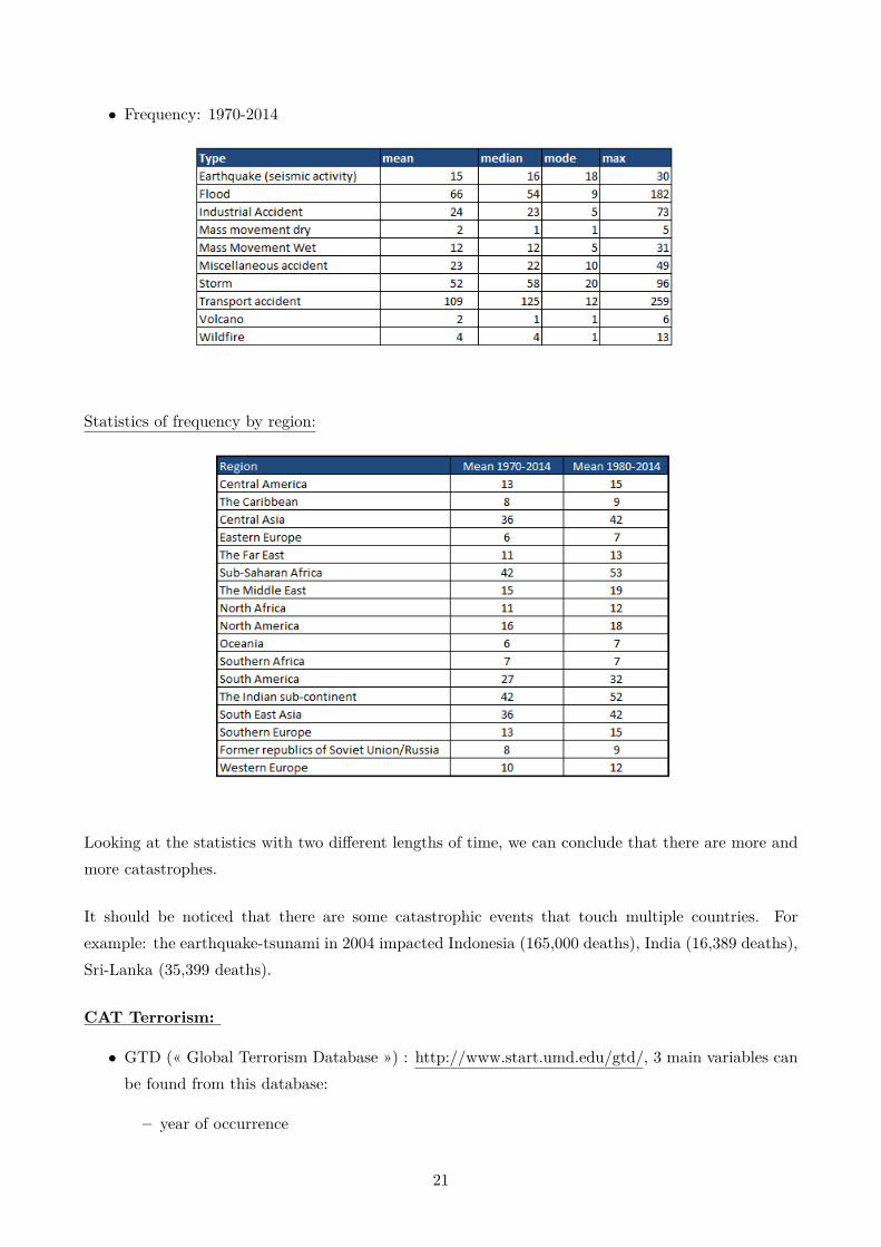
• Frequency: 1970-2014
Statistics of frequency by region:
Looking at the statistics with two different lengths of time, we can conclude that there are more andmore catastrophes.
It should be noticed that there are some catastrophic events that touch multiple countries. Forexample: the earthquake-tsunami in 2004 impacted Indonesia (165,000 deaths), India (16,389 deaths),Sri-Lanka (35,399 deaths).
CAT Terrorism:
• GTD (« Global Terrorism Database ») : http://www.start.umd.edu/gtd/, 3 main variables canbe found from this database:
– year of occurrence
21

– country name
– number of deaths
Figure 1.9: GTD database extration
1.3.3 The role of traditional reinsurance for a life insurer
Reinsurance plays very important roles in insurance activities and risk management:
• Protect the insurer against the occurrence of extreme events or the accumulation of many normalevents.
• Reduce the volatility of insurance portfolio.
• Increase the underwriting capacity of insurer. Reinsurance can help insurers underwrite the riskrequiring an amount of solvency capital greater than their own.
• Play the role as consulting. Reinsurer has sometimes more experiences and data in the marketdue to the fact that they work with many insurers at the same time. Reinsurer can thereforeprovide some services to insurer such as: launching new product, pricing, medical underwriting,etc.
1.4 Reinsurance in Solvency II context
1.4.1 Reinsurance in calculation of solvency capital requirement
1.4.1.1 Reinsurance under Solvency I
Solvency Margin and relief through reinsurance in Solvency I framework are measured very easilybased on factors on volumes and limited by arbitrary factors:
Solvency Margin = 4% of statutory reserves+ 0.3% of Sum At Risk
Capital relief through reinsurance as % of the Solvency Margin:
Min(reinsured reserves/ total reserves, 15%) +Min(Reinsured SAR/Sum At Risk, 50%)
22

1.4.1.2 Reinsurance under Solvency II
Under Solvency II, reinsurance has double effects which generally increase the SII Solvency Ratio:BOFSCR
• Reduction of Risk Margin leads to the increase of Basic Own Funds
• Reduction of SCR
Figure 1.10: Impact of reinsurance under Solvency II
23

Chapter 2
Non-proportional reinsurance pricingmodels
In this thesis, we aim to propose the reinsured risk-costing models for non-proportional reinsurance."Risk-costing" means that we do not set any margin above three traditional components of the price:pure premium, cost of capital and expense. We apply the proposed models in an example of reinsuranceprogram containing:
• XL per life treaty for per life level.
• XL per event (XL CAT) for the part retained net of the XL per life treaty.
The taken example uses an insurance portfolio based in France. The currency is EUR. The structuresof the reinsurance treaties are:
• XL per life: EUR 5M XL 1M. The number of reinstatement: 15.
• XL CAT: EUR 100M XL 10M. The number of reinstatement: 1. The minimum number ofvictims to trigger the treaty: 5.
The information for each kind of treaty is given as following:
XL per life: The treaty is priced for the 2017 coverage.List of data available and assumptions:
• 2010-2016 historical claims data above the retention of XL per life treaty including the develop-ment of claims
24

Figure 2.1: XL per life - List of claims higher than retention
Note that the amounts didn’t take into account inflation rate. They are reported amounts.
• 2010-2016 historical total ceded sum at risk
• 2010-2016 historical earned reinsurance premium
• Model point as in example in chapter 1
• Assuming that there is no special acceptance
• Assuming that there was no change in structure over past years
25
XL per event (CAT treaty): The treaty is priced for the 2017 coverage.List of data available:
• Total sum at risk and number of heads
• Sum at risk by range
• Model point in example in chapter 1
• Assuming that there is no special acceptance
• Concentration site information with the most concentrated groups in the portfolio.
2.1 XL per life
2.1.1 Some important definitions
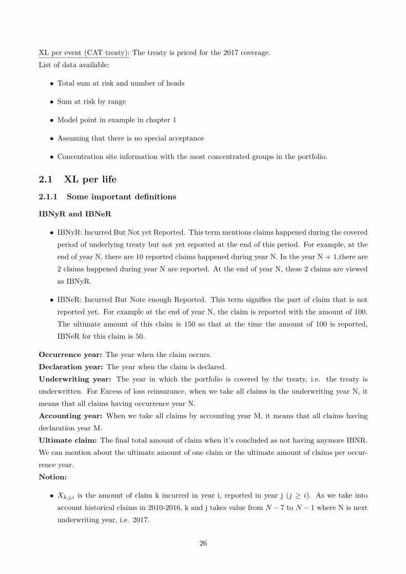
IBNyR and IBNeR
• IBNyR: Incurred But Not yet Reported. This term mentions claims happened during the coveredperiod of underlying treaty but not yet reported at the end of this period. For example, at theend of year N, there are 10 reported claims happened during year N. In the year N + 1,there are2 claims happened during year N are reported. At the end of year N, these 2 claims are viewedas IBNyR.
• IBNeR: Incurred But Note enough Reported. This term signifies the part of claim that is notreported yet. For example at the end of year N, the claim is reported with the amount of 100.The ultimate amount of this claim is 150 so that at the time the amount of 100 is reported,IBNeR for this claim is 50.
Occurrence year: The year when the claim occurs.Declaration year: The year when the claim is declared.Underwriting year: The year in which the portfolio is covered by the treaty, i.e. the treaty isunderwritten. For Excess of loss reinsurance, when we take all claims in the underwriting year N, itmeans that all claims having occurrence year N.Accounting year: When we take all claims by accounting year M, it means that all claims havingdeclaration year M.Ultimate claim: The final total amount of claim when it’s concluded as not having anymore IBNR.We can mention about the ultimate amount of one claim or the ultimate amount of claims per occur-rence year.Notion:
• Xk,j,i is the amount of claim k incurred in year i, reported in year j (j ≥ i). As we take intoaccount historical claims in 2010-2016, k and j takes value from N − 7 to N − 1 where N is nextunderwriting year, i.e. 2017.
26
• EPIk is the earned premium income of year k in the insurance portfolio which is used as anindicator for the basis of the volume of portfolio.
• ak is inflation rate of year k which is used as an indicator for the valuation of amounts in year k.
2.1.2 Pricing model
2.1.2.1 Grand principle
The premium for the XL per life treaty underwritten in year N is the combination of:
• Expected claim amount The expected claim amount in year N could be estimated by differentmethods:
– Frequency - severity
– Burning Cost
– Incident rates
– Combined method
In the following sections, we will go through each method and discuss their advantage andlimitation.
• Cost of capital or variance: When reinsurer underwrites a treaty, it takes risks. Therefore,an amount of solvency capital is required. Though the solvency required capital is normallycalculated in the portfolio level, an amount allocated per treaty should be taken into the price.The calculation of cost of capital per treaty will be described in chapter 3.
• Expenses: Once the treaty is signed, reinsurer has to spend fees on administration, acquisition,claim management, etc. The expense is often taken as fixed percentage of the commercialpremium for all treaties. In this thesis, we consider the expenses rate used in pricing is 10%.
2.1.2.2 Frequency-severity approach
We call the claims triggering XL per life retention or around the retention "atypical claims".Principle: The frequency of and severity of atypical claims incurred in year N are calibrated andthen simulated in 500K scenarios. The expected value of claim amount is taken as the average amountof 500K scenarios.We have:
S =N∑i=1
Xrei
Where:
• S is the annual reinsured claim amount
• N is the annual number of claims
27

• Xrei is reinsured amount of claim i
The price of XL per Life treaty is a composition of the expected value, the cost of risk which representsthe volatility of result undertaken by Reinsurer or the cost of require capital and the expense issuedby the management of the reinsurance treaty.
P = E(S) + Cost.of.risk
1− expense
The calibration of severity is done by 2 fitting methods: MLE (Maximum Likelihood Estimation) andMME (Method of Moment Estimation).
Maximum Likelihood Estimation (MLE)Suppose there is a sample x1 ... xn of n independent and identically distributed (i.i.d) observations,coming from a distribution with an unknown probability density function f(.). It is assumed that thefunction f belongs to a certain family of distributions {f(.|θ), θ ∈ Θ}, called the parametric model, sothat f = f(.|θ0). Θ is the definition interval of the function’s parameters. The value θ0 is unknownand is referred to as the "true value" of the parameter. It is desirable to find an estimator which wouldbe as close as possible to the true value θ0.To use the method of maximum likelihood, one first specifies the joint density function for all obser-vations. For an iid sample, this joint density function is:
f(x1, x2, ..., xn|θ) = f(x1|θ).f(x2|θ)...f(xn|θ)
The observed values x1, x2, ..., xn are fixed realizations of this function, whereas θ will be the function’sparameters and allowed to vary freely; this function will be called the likelihood:
L(θ|x1, x2, ..., xn) = f(x1, x2, ..., xn) =n∏i=1
f(xi|θ)
The log likelihood function is more often used in practice:
LL(θ|x) = ln(L(θ|x1, x2, ..., xn)) =n∑i=1
ln(f(xi|θ))
The method of maximum likelihood estimates θ0 by finding a value of θ that maximizes LL(θ|x). Thismethod of estimation defines a maximum-likelihood estimator (MLE) of θ0:
θmle ⊆ {argmaxθ∈ΘLL(θ|x)}
Method of Moment Estimation (MME)The method of moments is a method of estimation of population parameters such as the mean,variance, median, etc., by equating sample moments with unobservable population moments and thensolving those equations for the quantities to be estimated.Let (x1, x2, ..., xn) be an iid sample of the random variable X which is assumed to have a density where
28

is a vector parameter:Empirical mean of X is given by:
X = 1n
n∑i=1
Xi
Empirical variance of X, the unbiased estimator of the variance, is given by:
S2X = 1
n− 1
n∑i=1
(Xi − X)2
Empirical standard deviation of X = SX
Empirical distribution function of X = FX which is defined by :
∀x ∈ R, FX(x) = 1nCard{i ∈
[1;n
]/Xi < x}
Empirical α-quantile of X is defined by:
∀α ∈]0; 1], ˆF−1X (α) = Inf{x ∈ Supp(X)/FX(x) ≥ α}
Criteria to choose the best fitting quality distribution
• Akaike Information Criterion (AIC)
AIC = 2k − ln(L)
Where:
– k denotes the number of parameters of the statistical model
– L denotes the maximized value of the likelihood function
• Kolmogorov Smirnov criterion (KS)
The KS statistic quantifies a distance between the empirical distribution function of the sampleand the cumulative distribution function of the reference distribution.
Dn = supx|Fn(x)− F (x)|
• Cramer-von Mise
Let x1, x2, ...xn be the observed values in increasing order. The Cramer-von Mises criterion usesthe fact, that if is the underlying random variable X with the continuous distribution functionF (X), then F (X) follows the uniform distribution U(0, 1). Cramer-von Mise statistic:
T = 112n +
n∑i=1
[2i− 12n − F (xi)
]
29

• Anderson-Darling
The Anderson-Darling statistic:
AD = n
∫ ∞−∞
[Fn(x)− F (x)
]2[F (x)(1− F (x)]dF (x)
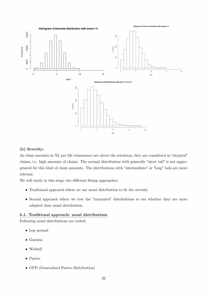
(a) Frequency:Frequency of atypical claims could be modelled by discrete distributions such as: Poisson, Binomialor Negative Binomial distributions. Each of them has different states of relationship between meanand variance, i.e:
• Negative Binomial: Mean ≤ Variance
• Poisson: Mean > Variance
The reason why we won’t use Binomial distribution is that it will simulate the number of claimslimited to a parameter n, which is not realistic.
Poisson distributionN is a Poisson random variable if it takes non-negative integer value: 0,1,2,... and its probabilityfunction is as following:
P (N = k) = λke−λ
k!Mean and variance:
E(N) = V ar(N) = λ
The parameter λ can be easily estimated by the empirical mean of the given sample.
Negative binomial distributionWe consider a sequence of independent trials with each following a Bernoulli distribution with proba-bility of success p in each trial. We are observing the sequence until there are r times of failure. Thenumber of success we have seen, K, will have Negative Binomial distribution. It takes non-negativeinteger value and its probability function is as following:
f(k, r, p) = P (K = k) = Ckk+r−1.pk.(1− p)r
Mean and variance:E(K) = rp
1− p = µ
V ar(K) = rp
(1− p)2 = σ2
By consequence, the parameters r and p are estimated easily by Method of Moment, i.e, with empiricalmean and variance of the given sample:
p = σ2 − µσ2
30

r = µ2
σ2 − µ
Consider that r →∞, denote mean of K as λ then
λ = rp
1− p ⇒ p = λ
r + λ
Hence, the probability mass function will be:
f(k; r, p) = Γ(k + r)k!.Γ(r) .p
k.(1− p)r = λk
k! .Γ(r + k)
Γ(r).(r + λ)k. 1(1+λ
r)r
If we consider r →∞ then Γ(r+k)Γ(r).(r+λ)k → 1 and 1
(1+λr
)r →1eλ
and finally,
limr→∞
f(k, r, p) = λke−λ
k!
which is the probability mass function of Poisson distribution.In other words:
Poisson(λ) = limr→∞
NB(r, λ
λ+ r)
The Negative Binomial distribution allows to take into account the over-dispersion problem (varianceis higher than mean) which can not be shown in Poisson distribution (where variance is equal to mean).
Binomial distributionWhen variance is observed to be smaller than mean, one can use the Binomial distribution. K is thenumber of successes in a sequence of n independent trials where each has the probability of success p.We note K follows a binomial distribution with parameters n ∈ N and p ∈ [0, 1], i.e, K ∼ B(n, p).The probability mass function of K is as following:
P (K = k) = Ckn pk(1− p)n−k
Mean and variance:E(K) = n.p
V ar(K) = n.p.(1− p)
Similar to the 2 frequency distributions above, the parameters of Binomial distribution can be easilyestimated by the empirical mean and variance of the given sample.The following histograms show the difference in variance of those distributions. The negative binomialdistribution gives larger dispersion than the Poisson distribution does and the binomial distributiongives the lowest dispersion.
31
(b) Severity:As claim amounts in XL per life reinsurance are above the retention, they are considered as "atypical"claims, i.e. high amounts of claims. The normal distribution with generally "short tail" is not appro-priated for this kind of claim amounts. The distributions with "intermediate" or "long" tails are morerelevant.We will study in this stage two different fitting approaches:
• Traditional approach where we use usual distribution to fit the severity
• Second approach where we test the "truncated" distributions to see whether they are moreadapted than usual distribution.
b.1. Traditional approach: usual distributionsFollowing usual distributions are tested:
• Log normal
• Gamma
• Weibull
• Pareto
• GPD (Generalized Pareto Distribution)
32
Log normal distributionX follows log-normal distribution with two parameter µ and σ that are respectively mean and standarddeviation of X if and only if:
X = eµ+σ.Z
where Z is standard normal random variable.Apparently, X has positive values.Probability density function:
f(x, µ, σ
)= 1xσ√
2πexp
[− (lnx− µ)2
2σ2]
The mean and variance of a random variable following a Log-normal distribution: Mean and variance:
E(X) = eµ+σ22
V ar(X) = e2µ+σ2(eσ2 − 1)
MLE
LL(µ, σ|x) = ln(L(µ, σ|x1, x2, ..., xn)) =n∑i=1
ln(f(xi|µ, σ)) = −∑i
(lnxiσ√
2π)−∑i
(lnxi − µ)2
2σ2
The MLE parameters optimizing this function are:
µ =∑ni lnxin
σ =n∑i
(lnxi − µ)2
n
MMEThe parameters µ and σ could be obtained by following equations:
µ = ln( E[X]2√
V ar[X] + E[X]2)
σ2 = ln(1 + V ar[X]E[X]2 )
By using the empirical mean and variance, we can calculate the corresponding estimators for µ andσ.
Weibull distributionThe cumulative distribution function of a Weibull variable X:
F (x, β, α) = 1− e−( xα
)β
for x ≥ 0 and F (x, β, α) = 0 for x < 0The probability density function:
f(x, α, β) ={
βα
(xα
)β−1e−( x
α)β x ≥ 0
0 x < 0
33

Where β > 0 is the shape parameter and α > 0 is the scale parameter of the distribution.The mean and variance of a random variable following a Weibull distribution:
E(X) = α Γ(1 + 1β
)
V ar(X) = α2[Γ(1 + 2β
)− (Γ(1 + 1β
))2]MLE
LL(α, β|x) = ln(L(α, β|x1, x2, ..., xn)) =n∑i=1
ln(f(xi|α, β)) =
The MLE method for Weibull requires some additional steps. We firstly recall the location-scaleproperty of ln(X):We note Y = ln(X) then the cumulative probability function of Y is:
P (Y < y) = P (ln(X) ≤ y) = P (X ≤ exp(y)) = 1− exp[−(exp(y)
α
)β]= 1− exp
[− exp
{(y − ln(α)
).β}]
= 1− exp[− exp
(y − ln(α)1β
)]= 1− exp
[− exp
(y − ub
)](b = 1
β, u = ln(α))
The corresponding sample of Y is: y1, y2, ..., yn yi = ln(xi)We have F (y) = 1− exp
[− exp( (y−u)
b )]
= G(y−ub ) with G(z) = 1− exp(−exp(z)) with g(z) = G′(z) =
exp(z − exp(z)). Thus,f(y) = F
′(y) = d
dyF (y) = 1
bg(y − u
b)
withln(f(y)) = −ln(b) + y − u
b− exp((y − u)
b)
As partial derivatives of ln(f(y)) with respect to u and b we get
δ
δuln(f(y)) = −1
b+ 1bexp(y − u
b)
δ
δbln(f(y)) = −1
b− 1b
y − ub
+ 1b
y − ub
exp(y − ub
)
and thus as likelihood equation:
0 = −nb
+ 1b
n∑i=1
exp(yi − ub
)
orexp(u) = [ 1
n
n∑i=1
exp(yib
)]b
and0 = −n
b− 1b
n∑i=1
(yi − ub
) + 1b
n∑i=1
yi − ub
exp(yi − ub
)
[5] shows that β is the root of following equation:
0 =n∑i=1
yiwi(β)− 1β− y where wi(β) = exp(yiβ)∑n
j exp(yjβ) withn∑i
wi(β) = 1
34

Then the estimation of β could be solved by numerical method.
MMEThe two first moments are:
m1 = (µ) = 1α
1β
Γ(1 + 1
β
)m2 = µ2 + σ2 =
( 1α
) 1β[Γ(1 + 2
β)− (Γ(1 + 1
β))2]
Then:σ2
µ2 =Γ(1 + 2
β )− Γ2(1 + 1β )
Γ(1 + 1β )
=Γ(1 + 2
β )Γ(1 + 1
β )− Γ(1 + 1
β)
Which depends only on parameter β. Therefore, the estimator of the shape parameter is obtainedusing the function:
h(c) =(1 + S2
x
x2
)(Γ(1 + 1
β))− Γ(1 + 2
β)
The MME estimator of β is the solution of h(β) = 0. After the estimation of β, the scale parameteris estimated by:
α =( x
Γ(1 + 1β
)
)βPareto distributionThe cumulative probability function of the Pareto random variable is as following:
FX(x) ={
1− (xmx )α x ≥ xm0 x < xm
The probability density function:
fX(x) ={
αxαmxα+1 x ≥ xm0 x < xm
The mean and variance of a random variable following a Pareto distribution:
E(X) ={∞ α ≤ 1αxmα−1 α > 1
V ar(X) ={∞ α ∈ (1, 2]( xmα−1)2. α
α−2 α > 2
MLElnfX(x) = lnα+ α.lnxm − (α+ 1)lnx
Hence,n∑i=1
f(xi|α) = n.lnα+ n.α.lnxm − (α+ 1)n∑i=1
xi
The MLE estimation of parameter α is the solution of the equation:
35

δ
δα
n∑i=1
f(xi|α) = n
α+ nlnxm −
n∑i=1
lnxi = 0
Hence,α = n∑
i lnxi − n.lnxmMMEThe MME estimation of α is deduced by the first moment equation.
αMME = x
x− xmGeneralized Pareto DistributionThe cumulative distribution function of random available X following the Generalized Pareto Distri-bution:
F(ξ,µ,δ)(x) =
1−(1 + ξ(x−µ)
δ
)− 1ξ
for ξ 6= 01− exp(−x−µ
δ ) for ξ = 0
The probability density function:
f(ξ,µ,δ)(x) = 1δ
[1 + ξ(x− µ)
δ
](− 1ξ−1)
for x ≥ µ when ξ ≥ 0 and µ ≤ x ≤ µ− δξ when ξ < 0
The mean and variance of a random variable following a Generalized Pareto Distribution:
E(X) = µ+ δ
1− ξ , ξ < 1
V ar(X) = δ2
(1− ξ)2(1− 2ξ) , ξ <12
If ξ ≥ 1/2 variance doesn’t exist, if ξ ≥ 1 even mean doesn’t exist.
With shape ξ > 0 and location µ = σ/ξ , the GPD is equivalent to the Pareto distribution withscale xm = σ/ξ and shape α = 1/ξ.MLE
LL(u, σ, ξ|x)n
= −ln(σ)− (1 + 1ξ
).n∑i=1
ln(1 + ξ
xi − µσ
)We take ρ = ξ
σ , then estimator of ξ and ρ are solution of:
(ξ, ρ) = argmax{−ln(ξρ
)− (1 + 1/ξ).n∑i=1
ln(1 + ρ(xi − µ))}
MMEThe estimators of ξ and σ are:
xi = 12[1− (x− µ)2
S2x
]
36

σ = 12(x− µ)
[1 + (x− µ)2
S2x
]b.2. Truncated distributionsWhy truncated distribution?In statistical theory, we knew about usual distributions for extreme value studies, for example: Weibull,log-normal, log-gamma, etc. However, those distributions have ranges of variable’s values in entireset R or R+ while as discussed previously, we’re interested in atypical claims, i.e, whose amounts arehigher than certain thresholds. That’s why we will analyse the use of the "truncated distributions" -whose range are bounded at some levels.Definition:If g(x) and G(x) is the density and cumulative distribution functions of a random variable X, thenthe density distribution function of the truncated variable Y = X/a<X<b is as following:
fY,a,b(x) = g(x)G(b)−G(a) ∗ Ia≤x≤b
Note from this formula that f(x) has exactly the same parameters as g(x).In our case, we will use left-truncated distribution since our data accepts values in the interval [R,+∞) where R is the threshold of atypical claims.We call g(x) as original distribution, and f(x) as truncated distribution.The following example shows the difference between the original distribution and its truncated version:Example 1: two-side truncated logistic distribution and logistics distribution.Following is the histogram of X with logistics distribution and Y with truncated logistics distribution.Its parameters are:
• Location = 0
• Scale = 2
37

Figure 2.2: Example of truncated distribution - Logistic distribution
The density of Y concentrates in the interval (-5, 5) that makes higher density values of Y in thisregion than density values of X.
Cumulative probability function and inverse probability function are defined as following:
FY (x) = G(max(min(x, b), a))−G(a)G(b)−G(a)
F−1Y (p) = G−1(G(a) + p.(G(b)−G(a)))
The mean and variance are calculated as following:
E(X) =∫ b
axfX(x)dx
,
V ar(X) =∫ b
a{x− E(X)}2fX(x)dx
In this document, one of our objective is to compare the efficiency of left-truncated distributions andtheir usual version in fitting severity of atypical claims. We will try to test the following truncateddistributions:
• Left-truncated Log-normal
• Left-truncated Weibull
Left-truncated Log-normalWe consider the variable X following left-truncated log-normal distribution then X ∈ [u,+∞].Mean and variance:
E(X) = u+ exp(µ+ σ2
2 )
38

V ar(X) = exp(2.µ+ σ2).(exp(σ2)− 1)
MLEThe MLE estimators for µ and σ are:
µ =n∑i=1
ln(xi − u)
σ = n
n− 1
n∑i=1
[ln(xi − u)− µ
]2MMEThe estimators MME for µ and σ are:
σ2 = ln[1 + ( S2
x
x− u)2]
µ = ln(x− u)− σ2
2Left-truncated WeibullThe cumulative distribution function of left-truncated Weibull:
F (x) =[1− exp
(− (x− u
α)β)]
Where u is the atypical thresold, β the shape parameter, α the scale parameter.The mean and variance are given by:
E(X) = u+ α.Γ(1 + 1
β
)
V ar(X) = α2[Γ(1 + 2β
)− (Γ(1 + 1β
))2]Similar to the usual version Weibull distribution, we obtain following estimators of α and βMLEThe shape parameter c is the solution of h(β) = 0 where:
h(β) =
∑ni=1
((xi − u)β.ln(xi − u)
)∑ni=1(xi − u)β − 1
β−
n∑i=1
(xi − u)β
Then the estimation of the scale parameter is:
α =[ n∑i=1
(xi − u)β] 1β
Advantage and limitationAdvantage
• This method helps to have very good views on frequency and severity of claim amounts. It helpsto predict better the tail of the distribution of claim amounts.
39
• When there are few claim data higher than the retention, external or internal reinsurer mayask for claim amounts lower than the retention and use this method to simulate claim amounthigher than the retention.
Limitation
• It’s not applicable when there is no possibility to obtain sufficient claim data.
• The model is purely based on claim data therefore doesn’t consider the risk profile of the portfolio(age, sum at risk distribution, etc.)
2.1.2.3 Burning Cost method approach
Definition: “Burning Cost ratio”Burning Cost ratio for underwriting year N is ratio between the ultimate claim amount occurredduring year N and the exposure basis of year N. The earned premium income or the total sum at riskof year N could play the role as “exposure basis” which represents the size of portfolio. The largerportfolio is likely to have bigger ultimate claim amount.
BCi = Si/Ci
Where: BCi, Si and Ci are the burning cost ratio, the ultimate claim amount and the exposure basisfor underwriting year i.The “exposure basis” isn’t obliged to be the earned premium income or total sum at risk. One canreplace it by another indicator which allows having a reference of the development of insurance/rein-surance portfolio, for example: the total ceded Sum at Risk.If we use “The total Sum at risk” as “exposure basis” for the calculation of burning cost ratio of areinsurance portfolio:
BCi = SiSARi
Where:
• Si is the total ultimate reinsured claim amount occurred during year i
• SARi is the total SAR in the underwriting year i
Reinsurance pricing XL per life by Burning Cost ratio Principle: The burning cost ratio forthe pricing underwriting year is estimated by the (weighted) average of last n years burning cost ratio.
BCN = 1n.(BCN−1 +BCN−2 + ...+BCN−n)
Or, weighted average by premium basis:
BCN = BCN−1.CN−1 +BCN−2.CN−2 + ...+BCN−n.CN−nCN−1 + CN−2 + ...+ CN−n
40

Finally, the pure premium is calculated by:
E(S) = BCN ∗ SARN
Calculation of IBNRIn the numerator of the Burning Cost ratio, we have to calculate the "ultimate" amount of claimsoccurred in the year. The current information gave the view at 31/12/N-1. Wae have to estimate thelevel of IBNR of reinsured claims at this time. There is a number of traditional approaches for theestimation of IBNR, for example: Chain ladder, Bonheuter Ferguson, Boostrap. However, from thepractical point of view, we will consider in this thesis the Chain ladder approach which is deterministicand easy to use.As mentioned, the estimation of IBNR consists two parts: IBNyR (Incurred But Not yet Reported)and IBNeR (Incurred But Not enough Reported).IBNyRThe chain ladder method applies to the number of claims Mi,j triangle.
Figure 2.3: Number of claims triangle
The development factor of the number of claims from year j to year j +1:
fj =∑n−ji=1 Mi, j + 1∑n−j
i=1 Mi,j
, j = 1, . . . , n− 1
Where Mi,j is the number of claims occurred in year i and reported before or in year j.From the development factor we can estimate the ultimate number of claims:
Mi,n = Mi,n−i+1 ×n−1∏
j=n−i+1fj
IBNeRThe IBNeR effect takes into account the development in terms of amount of occurred claim.
gj =∑n−ji=1 Si, j + 1∑n−j
i=1 Si,j, j = 1, . . . , n− 1
41
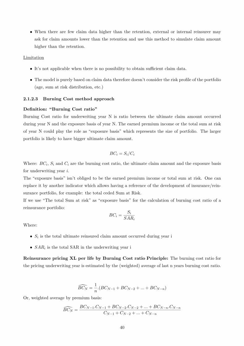
Where Si,j is the total amount of claims occurred in year i and reported before or in year j. Itmeans, we consider also the development of late declared claims. The "double" triangle is used for thecalculation of Chain-ladder factors:
Figure 2.4: Amount of claim triangle
Ultimate claim amountsAs in deterministic approach, we don’t aim to add "new claim" in the list, we will apply both IBNyReffect and IBNeR effect in the claim amount. We have the ultimate single claim amount:
Xi,n = Xi,n−i+1 ×n−1∏
j=n−i+1fj ×
n−1∏j=n−i+1
gj
The ultimate reinsured claim amount of the year of occurrence i:
Si =Ni∑Xi,n
Where Ni is the number of claims occurred in year i.Remark: "AS-IF" calculation for Burning Cost approach:The ultimate claim amounts and exposure basis should be recalculated in order to have equivalentvalues in the current year (N) (taking into account inflation impact). This "AS-IF" calculation isdescribed in the section 2.1.3.3.Finally, we have the result for pure premium:
E(S) = BCN ∗ SARN
However, this deterministic methode doesn’t give us a view on volatility of reinsured annual claimamount. The Cost of capital part in the pricing formula could be calculated by using a hybridapproach: using life shock described in Appendix A.
Advantage and limitationAdvantage
• It’s deterministic approach which is easy to implement and it helps to have a global view on theclaim amounts.
• In case that there are few claims, the Burning Cost method can still give a price.
Limitation
42

• The Burning Cost approach bases only on the historical claims, it doesn’t consider the detail onthe exposure of portfolio (age, volatility of SAR, number of insured, etc.)
• The approach is not suitable when there are no historical reinsured claims. When there are fewclaims, the method still works but the result isn’t very reliable due to the fact that in general,reinsurance claims are very volatile, the method doesn’t help to predict potential reinsuredclaims.
• The Burning Cost approach is a deterministic approach which relies on the average of annualresults therefore it doesn’t take into account the volatility of reinsured claim amount.
2.1.2.4 Incident rate approach
Sometimes, the XL per life treaty isn’t working and we don’t get enough claim data to performfrequency and severity model. The Burning Cost method can give in some cases a price but it has thelimitation to do not take into account the portfolio’s risk profile and volatility of claims.In the data communicated by insurer, we can obtain a model point of the insurance portfolio: theaverage age and the number of insured per range of SAR, i.e:
Figure 2.5: Model point for XL per Life pricing
Methodology:Assuming that we can obtain the mortality Best Estimate of the mortality insurance portfolio, i.e. qxitable, for each range of sum at risk i, the random variable amount of claims follows a binomial law.We have following parameters applied in the method:
• The total number of experiments, i.e. the number of insureds Ni
• The probability of death, qxi
Given SARrei , the average sum at risk of the range, the mean and variance of the reinsured claimamount belonging to the range i are calculated by:
• E(Xi) = qxi .Ni.SARrei
43

• V ar(Xi) = qxi .(1− qxi).Ni.SARrei2
It is then possible to sum all those variables together to get the amount of claims ceded to reinsurer.
• E(S) =∑i qxiNiSARrei
• V ar(S) = V tMV with V the vector of standard deviation of X and M the matrix of covariancereflecting the dependency between bands (correlation assumed).
The pricing formula could be the traditional combination of mean and variance:
P = E(S) + βσ(S)1− expense
Advantage and limitationAdvantage
• The incident rate approach takes into account the portfolio’s information such as age, averageSAR per range, etc.
• Compared to Burning Cost approach, mortality incident rate approach gives an idea about thevolatility of the claim amount.
• The method works even when we have very few claim data
• Simplicity of the calculation: Once mortality Best Estimate rate is available, the expected valueand variance of the claim amount are calculated quite easily.
Limitation
• There is a basic risk in the calculation. The Best Estimate mortality rate represents the insuranceclaims while we are in the issue of estimating reinsured claims. The mortality rate may be lowerbecause of a better underwriting process for high sum insured cases. It doesn’t fully take intoaccount historical reinsured claims.
2.1.2.5 Combined approach
The combined approach between Burning Cost which uses the historical reinsurance claim and theincident rate approach which uses the portfolio information (age, average SAR per range, etc.) couldhelp to use the maximum amount of available information.Principle: We suppose that the historical reinsured claim information represents correctly the averageclaim amount but it doesn’t sufficiently illustrate the variance, for example, due to limited claim data.The idea is to keep this average view and use the variance view given by the qx Best Estimate asdescribed in incident rate method.Methodology:From the historical claim amount, we determine the Best Estimate mortality of reinsured portfolio.
44

qREx = Sreal
SInsuranceBest.Estimate
× qxInsuranceBest.Estimate
Where:
• qREx is the Best Estimate mortality rate for reinsured claim
• Sreal is the historical amount of reinsured claim
• SInsuranceBestEstimate is the hypothetical reinsured claim amount calculated by using qx Best Estimateof insurance portfolio (as in the section "incident rate approach")
• qxInsuranceBestEstimate is the qx Best Estimate rate of the insurance portfolio
Once the qREx is calculated, the price is then calculated in the same way as in the incident rateapproach.Advantage and limitationAdvantage
• It takes into account both historical reinsured claim information and portfolio information.
Limitation
• It doesn’t keep the view in variance shown by historical reinsured claims information as thefrequency-severity does. However, when the variance of reinsured claims view is judged as notcreditable (for example, due to limited claim data, the treaty is not very working, etc.), we canconsider that this limitation is not significant.
2.1.3 Application of proposed pricing models
2.1.3.1 Data
We will consider the XL per Life reinsurance treaty as described at the beginning of the chapter. Theinformation given in a Renewal period to reinsurers are as following:
• Contractual elements: Draft of reinsurance treaty with condition terms such as: Retention,Limit, the number of reinstatement, etc.
– Retention: 1M
– Limit: 5M
– Number of reinstatement: 15
• Historical claim amounts above the retention level containing:
– Amount of claim at 1st declaration date
45

– Date of occurrence. Claim historic from 2010 to 2016. In practice, the year 2016 isn’tcomplete as the Renewal period takes place normally before year end. It requires in themodelling some treatment for example: proportionally adding the claim amount in orderto obtain full year claims. However, in this case study, for the sake of simplification, weassume the claim data is updated to full year 2016.
– The claim amount and status (open/closed) at the end of each year
• Portfolio profile: The model point presented in chapter 1 is used:
• The earned premium income for the period 2010-2016 and the expected premium income for2017:
• The total SAR for the period 2010-2016 and the expected SAR for 2017.
2.1.3.2 Claim data descriptive statistics
Frequency development 2010-2016:The following triangle contains frequency development information of claims above retention 1M withoccurrence year and development year viewed at 31/12/2016. Note that the number shown in thediagonal is the number of claims known at 31/12/2016.
46

Severity viewed at present year:The following tables shows some descriptive statistics about the gross amount of claims (before rein-surance) viewed at 31/12/2016:
We should notice that in the claim data, there are "closed" claims which are considered to no longerdevelop and "open" claims which would have potentially IBNeR amount in the future. The number of"closed" and "open" viewed at 31/12/2016 are resumed in the following table:
We can see that all claims occurred in 2010 and 2011 are all considered as "closed". This situation isvery common in death claims: in general, all claims are reported and closed after 5 years or less.
2.1.3.3 Pricing
a) Frequency - severity approach
Frequency fitting:Step 1: Determining the ultimate number of claims:By using Chain-ladder we can estimate the ultimate number of claims by occurrence year. This stephelps us take into account the IBNyR effect.
The IBNyR development factor from N+i to N+i+1:
The IBNyR development factor from each occurence year to it’s ultimate number:
47

Step 2: Fitting the ultimate number of claims
The ultimated number of claims is fitted with Poisson or Negative Binomial distribution. As thenumber of data points is small, the MME method could be used.As E(N) = 8 > V ar(N) = 2.3, the chosen distribution should be Poisson with parameters: λ = 8
Severity fitting:Step 1: Estimation of IBNeR effectThe IBNeR development factor from N+i to N+i+1:
The IBNeR ultimate development factor of claims for each occurrence year to it’s ultimate amount:
From the IBNeR development factors given by method Chain-ladder, we can see that claims occurredbetween 2010 and 2014 will no longer develop.
Step 2: Taking into account inflationGiven the inflation rate, we could calculate also the inflation impact based on a 100-scale index:
48

Step 3: Taking into account evolution of portfolio exposure. Final AS-IF claim amountGiven the total SAR per information, we can calculate the impact of the evolution of portfolio exposurebased on a 100-scale index:
The final AS-IF claim amount is calculated by applying the inflation index and portfolio exposureindex. The coefficients are calculated per occurrence year as following:
These coefficients are to be applied to the claim amount in order to have the AS-IF amounts. It meansthat a claim amount X occurred in 2010 is equivalent to a claim amount of 1.16 × X in 2017. Thefollowing table shows the list of 10 largest claims and their AS-IF amount.
The AS-IF claim amounts are taken as the sample of the calibration of severity. As mentioned above,6 distributions are tested:
• Log-normal
• Weibull
49
• Left-truncated Log-normal
• Left-truncated Weibull
• Pareto
• Generalized Pareto Distribution
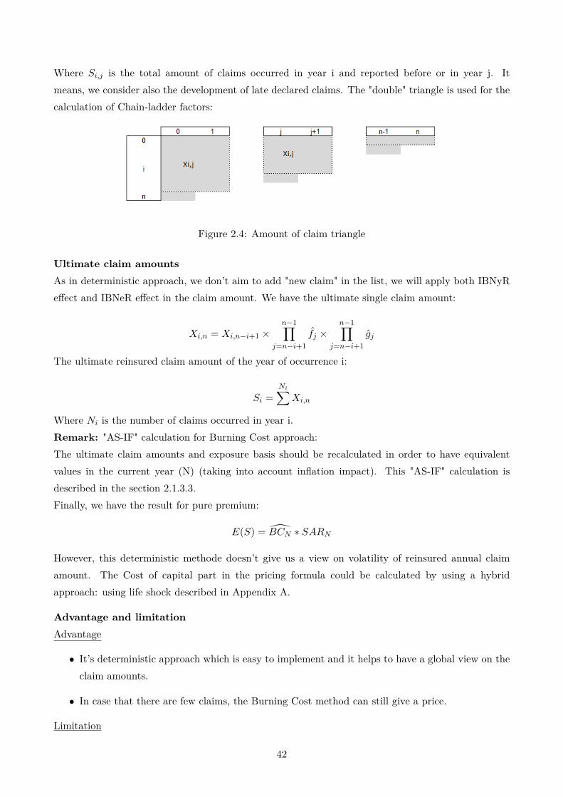
We have following result for goodness of fit criteria:
Figure 2.6: Goodness of fit criteria
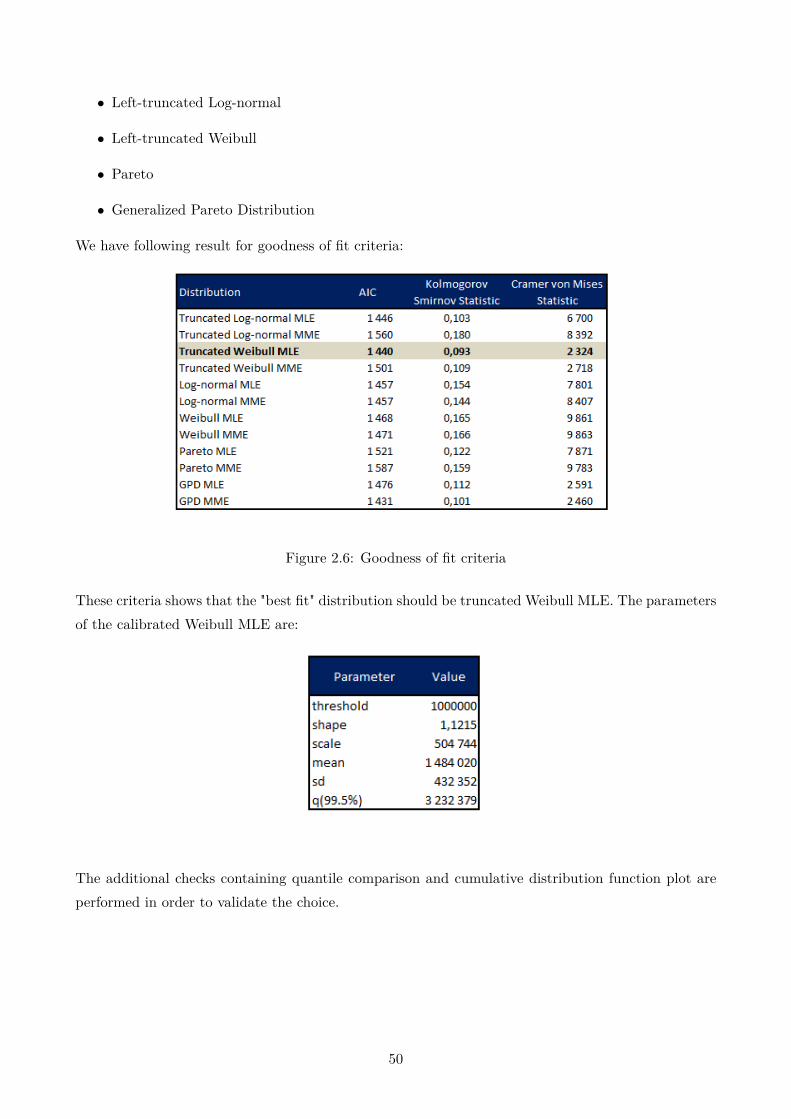
These criteria shows that the "best fit" distribution should be truncated Weibull MLE. The parametersof the calibrated Weibull MLE are:
The additional checks containing quantile comparison and cumulative distribution function plot areperformed in order to validate the choice.
50

Figure 2.7: Truncated Weibull cumulative distribution function
Looking at the quantile comparison in the table above, the truncated Weibull distribution gives moreprudence in the tail of the distribution and very good fit in the beginning part of the distribution. Inaddition, given the fact that the existed claims are only at the first ranges of Sum At Risk, we validatethe truncated Weibull distribution.It is interesting to compare the goodness of fit of truncated Weibull with its original (non truncated)version of the distribution:
51
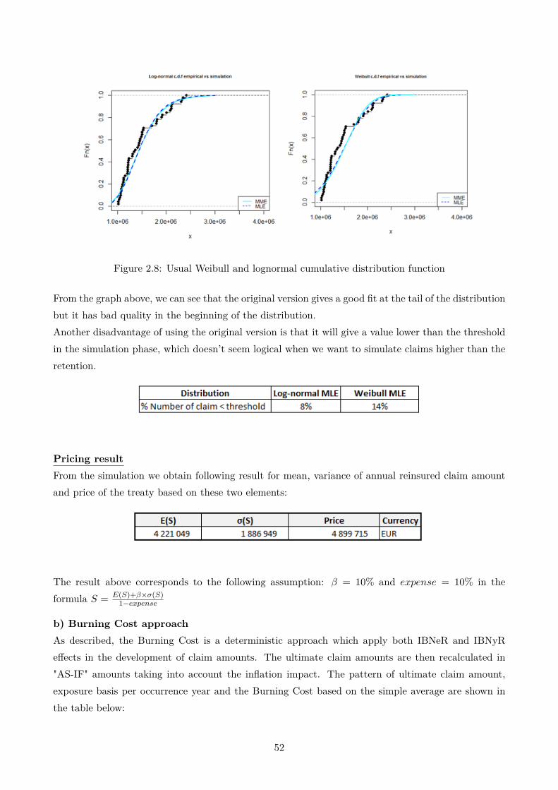
Figure 2.8: Usual Weibull and lognormal cumulative distribution function
From the graph above, we can see that the original version gives a good fit at the tail of the distributionbut it has bad quality in the beginning of the distribution.Another disadvantage of using the original version is that it will give a value lower than the thresholdin the simulation phase, which doesn’t seem logical when we want to simulate claims higher than theretention.
Pricing resultFrom the simulation we obtain following result for mean, variance of annual reinsured claim amountand price of the treaty based on these two elements:
The result above corresponds to the following assumption: β = 10% and expense = 10% in theformula S = E(S)+β×σ(S)
1−expense
b) Burning Cost approachAs described, the Burning Cost is a deterministic approach which apply both IBNeR and IBNyReffects in the development of claim amounts. The ultimate claim amounts are then recalculated in"AS-IF" amounts taking into account the inflation impact. The pattern of ultimate claim amount,exposure basis per occurrence year and the Burning Cost based on the simple average are shown inthe table below:
52

The pure premium is the product of average burning cost and the expected exposure basis of 2017.Pure premium given by Burning Cost approach: EUR 4,728,270. The reinsurer can add their cost ofcapital and expense into the price. The cost of capital is calculated as described in appendix A (atabout EUR 445, 952 × 110% = 490, 547 assuming a transmission factor of 110%). Finally, we havereinsurance premium at about EUR 5, 798, 686
c) Incident approachExpected value and the variance of annual reinsured claim amount calculated by qx Best Estimateinsurance can be shown in the following table:
Figure 2.9: Incident approach
Suppose that there is no correlation between different ranges of SAR, then V ar(S) =∑i V ar(Xi).
In final, we have:
• E(S) = 15.7m
• σ(S) = 5m
If we apply the same pricing formula as in the frequency-severity approach (β = expense = 10%),then we have P = 17.9m.This price has only indicative sense since it has no link with the historical reinsured claim amount.
d) Combined approach
53

The combined approach between Burning Cost and incident rate uses both results of two approaches.From the expected annual claim amount estimated in Burning Cost and incident rate approaches, weestimate the discount rate in qx Best Estimate:
qREx = 4.715.7 × q
BEx = 30.1%× qBEx
By using the same calculation as in the incident rate approach and the same pricing formula withβ = expense = 10%, we obtain:
• E(S) = 4.7 m
• σ(S) = 2.7 m
• Final premium = 5.56 m
e) ConclusionIn summary, we have following results given by 4 approaches:
Figure 2.10: Summary - results of XL per life reinsured risk-costing models
(*): All prices are calculated based on the same pricing formula using pure premium, standard devi-ation and expense except for Burning Cost approach as this deterministic approach doesn’t calculatethe variance.We have following conclusion:
• The frequency and severity approach purely based on the historical reinsured claim information.Its outputs are therefore expected value and variance based on historical amounts.
• The Burning Cost approach also purely based on the historical reinsured claim information.However, it’s deterministic approach which applies both IBNeR and IBNyR effect on the claimamount viewed at 31/12/N-1. The method doesn’t calculate the variance of annual reinsuredclaim. The price is calculated based on pure premium and cost of capital estimated from ahybrid method (life shocks for SCR and PC approach for pure premium).
• The incident rate approach in this case has only indicative purpose because it takes into accountonly the portfolio information, the best estimate mortality view is based on insurance portfolio(for internal reinsurer) and reinsurer’s experience in the market (for external reinsurer).
• Combined method between Burning Cost and Incident Rate could help to return to the expectedclaim amount level as in Burning Cost calculation and in addition, to have a view on variancewhen there are few historical claims.
54

From the different views on the price, an internal reinsurer could be able to define their strategy ofcession and an insurer can challenge the price of external reinsurers.
2.2 XL per event
2.2.1 Risks covered by XL per event (CAT treaty)
The CAT treaty covers following risks:
• Earthquake
• Tsunami
• Flood
• Storm
• Volcanic activities
• Forest fires
• Industrial hazard
• Terrorism
And the following risks are not covered by CAT treaty:
• Famine
• Epidemic, pandemic
• Extreme temperature
• Drought
The reason for that they are not covered is these types of event normally happen during a long periodand it’s difficult to conclude exactly the cause of the death for a big number of victims.
2.2.2 Treaty conditions
The treaty CAT covers accidents caused by the types of events mentioned above but there are inaddition other conditions for example:
• The CAT event occurs in the covered period of the treaty, i.e. from 1 January to 31 December;
• There are at least M victims caused by the event and the amount of claim exceeds the retentionof the treaty. In general, M is often taken between 3 and 5 deaths.
• The CAT treaty covered victims during first three days of the event. After that, it’s oftenconsidered as a second event.
55

2.2.3 Data analysis
We recall the available data for the pricing of CAT treaty:Portfolio data:
And,
Contractual elements:
The treaty covers both natural catastrophes (CAT NAT), terrorism events, and also man-made nonterrorism events (traffic accidents, industrial accidents, etc.)
Public catastrophes database - EMDATEMDAT database contains historical natural and man-made non terrorism catastrophic events.The treaty covers an insurance company based in France. As at the renewal period, we don’t havethe full year 2016 database, we suppose to use the historical catastrophic events during the period1970-2015 in order to calibrate the risk. We don’t consider the events happened before 1970 to makesure that the data is enough reliable and that we have the similarity of condition (infrastructure,prevention, etc.) as today.
Frequency:
56

In average, there are 3 events per year are recorded in EMDAT.
Severity:
It’s interesting to note that the median and mean are far lower than the max. In order to have abetter view on the number of victims, we plot them per occurrence year:
57

There are 6 events with more than 100 deaths in the tail of the sample. Most of the remaining eventsconcentrate in the range [1, 50]. The median of the number of deaths is 11.
Public terrorist acts database - GTDFrequency:
The graphic above shows that there were a lot of terrorist acts in the period 1975-1995 then it wasvery few events until recent period. However, in 2015, it was suddenly recorded the largest number of
58

terrorist acts in France (15 attacks).
Severity:
The graph above about fatality of terrorist acts in France shows that almost all of events have lessthan 20 deaths. There is only one irregular point: 92 people were killed in Bataclan attack.
Population:The population of France is taken from http://data.worldbank.org/ with 66.8 millions of inhabitantsin 2016.
2.2.4 Pricing model
2.2.4.1 Deterministic model
When we say "deterministic", it means the method doesn’t require Monte-Carlo simulation.One of the first pricing models was developed by Strickler (1960): The reinsurer obligation is modeledby 2 factors:
• The frequency distribution of the events which cause more than M deaths
• The distribution of the reinsured claim amount
Distribution of claim amount:Denote C the claim amount of one insured life in a CAT event. ¯SAR the average sum at risk per head.According to Strickler’s assumption, C follows the following distribution: C ∼ SAR × Exp(1) whereExp(1) is the exponential distribution with mean 1. Then, in an event of n deaths, the total claimamount of this event, denoting by Z, follows the following distribution: Z ∼ SAR × Γ(n, 1) where
59
Gamma(n, 1) is Gamma distribution. The underlying assumption here is the claim amounts per lifein one CAT event are independent, then the sum of independent exponential distribution is a Gammadistribution.If wn(z) is the density distribution function of Z, then:
wn(z) = ezzn−1
(n− 1)!Number of victims:By analyzing the SBMLIC database (Statistical Bulletin of the Metropolitan Life Insurance Company),Strickler found that the annual number of victims among 1 million people of the general populationdue to CAT events with more than n deaths could be estimated by:
A(n) = 8× 1001/n × n1/3
A(1) represents the total number of victims over 1 million people due to CAT events during the year.
The annual number of CAT events:The number of CAT events which cause exactly n deaths over 1 million people of general populationis calculated by:
H(n) = A(n)−A(n− 1)n
Hence, the probability that an event causes exactly n deaths when it occurs is:
h(n) = H(n)∑∞i=0(H(i))
Note that when n → ∞, H(n) → 0 and h(n) → 0. Strickler used a conservative assumption thatH(n)→ 0 when n > 1500.
Distribution of the claim amount:As mentioned, in CAT treaty, the reinsurer will pay only when the event causes from M deaths. Thedensity probability function of the amount of claim:
w(n) =∞∑
n=Mh(n)wn(z)
Limitation of the Strickler model:
• The function A(n) is predefined and applied only for the US database at the giving time of theextraction of data.
• The assumption that H(n) = 0 when n > 1500 is a strong assumption. In history, it exists someCAT events that cause a much higher number of death. Example: Tsunami in Indonesia in 2014killed 165,708 people.
• The assumption about the claim amount which follows Gamma distribution is a strong assump-tion.
Strickler model has strong assumption but given the availability of data at that time, it alreadydemonstrated a good approach and give us the idea to develop new model.
60

2.2.4.2 Model by simulation
Erland Ekheden (2008) published in his thesis new model which at the same time reuses Stricker’sideas and takes into account some improvements compared to Strickler’s model:
• The frequency and severity of CAT events are calibrated from an international source of data
• The distribution of claim amount divided by the average sum at risk is again assumed to beGamma distributed
Notion:
• K: the number of catastrophic events occurred during the period of contract (we consider thecase of 1 year period);
• Xk: the number of victims in the general population due to kth event.
• Yk: the number of victims in the insured portfolio
• Zk: the amount paid by the insurer for the event k
• Zrek : the amount paid by the reinsurer for the event k
• SARind: the average sum at risk of individual business
SARind = Total sum at risk individual businessTotal number of heads individual business
• SARgrp: the average sum at risk of group business
SARgrp = Total sum at risk group businessTotal number of heads group business
• SAR: The average sum at risk of the whole portfolio (both individual and group)
• q: insurance penetration rate
q = the number of insuredpopulation of the covered zone
• pr.region: sub-region penetration rate
pr.region = population of the covered zonepopulation of the simulation zone
• R: retention of the treaty
• L: limit of the treaty
Frequency:Note Km the number of CAT events which cause at least m deaths in the calibration region. Wesuppose that Km is:
61

• A Poisson variable if E(Km) ≥ V ar(Km)
• A Binomial Negative distribution if E(Km) < V ar(Km). In general, we observe a over-dispersion(variance > mean). The BN distribution gives us this property.
The parameters of frequency are calibrated easily by the method of moment.In some cases, depending on the countries, the covered zone doesn’t contain enough data, we have tocalibrate based on a larger region by adding some neighbor countries.Example: Luxembourg. We would regroup it with Germany, France, Belgium. We note « the region»: Luxembourg, Germany, France, Belgium and « the sub-region » : Luxembourg.The the pr.region parameter is used:
pr.region = population of the covered zonepopulation of the simulation zone
We note Jm the number of CAT events which cause at least m deaths in the covered region:
Jm ∼ Binom(Km, pr.region)
Severity:We suppose that the severity in sub-region has the same characteristic as in the region. We calibratethe parameters of severity distribution in the regional level. We note X the number of deaths in theregion due to a CAT event. X can receive extreme values in the tail of distribution. Therefore, wecan model X by a GPD (Generalized Pareto Distribution):
X ∼ GPD(m,σ, ξ)
We note Y the number of death in the insured portfolio due to the event that caused X death in theregion. .We suppose that given X, Y follows Binomial distribution.
Y |X ∼ Binom(X, p)
In order to take into account the dependency of victims in a CAT event, we introduce here a parameterθ.Then, p follows Beta distribution given X:
p|X ∼ Beta(qθln(X), (1− q)θln(X)), θ ∈ R
where q is the insured penetration rate: q = total number of insuredspopulation of the covered zone
Remark:
• if θln(X)→∞ then Y |X ∼ Binom(X, q)
• if θln(X)→ 0 then P (Y = 0|X) = 1− P (Y = X|X) = 1− q
62

The parameter θ represents dependency. A small θ implicates high dependency and a big θ implicatesthe independence among the victims.
The reinsured claim amount due to CAT events:In Erland Ekheden’s thesis, the Strickler’s assumption is applied. The amount of claim paid by theinsurer follows gamma distribution multiplied by the average sum at risk per head.
Z = SAR× Γ(y, 1)
Application of reinsurance treaty:
Zre = min(max(Z −R, 0), L)1Y >=m
Hence, the annual reinsured claim amount:
S = min(Jm∑i
Zrei , AAL)
Pricing formula:It should take into account following main components: pure premium, cost of required capital,expense, number of reinstatement:
Pfinal = PP + CoC
(1− expense) ∗ freinstatementWhere:
• PP: Pure premium
• CoC: Cost of capital
• freinstatement: factor which represents the fact that insurer has to pay reinstatement premium.
Reinstatement factor:In order to quantify the impact of reinstatement, we consider following consequent cases:a) We consider the following reinsurance contract: L XS F (without AAL or reinstatement).S is the sum of N claims of reassured amounts Yi,i=1..N , i.e.
S =N∑i=1
Yi
where Y is the reassured amount for sinister X:
Y = min[max((X − F ), 0), L]
In this case, we can say that there is no limit for S in a year, when N →∞ then S →∞.The pure premium of reinsurance:
P1 = E(S)
63

b) We consider the following reinsurance contract: L XS F @ 1 reinst 0 % (free reinstatement).Note that in this case, the reinstatement is free and AAL = (1 + nb.of.reinst) ∗ L = 2L.We denote S′ the total annual charge for the reinsurance company, we get:
S′ = Min [S, AAL] = Min [S, 2L]
Then we get the premium P2 for this 1 free reinstatement treaty:
P2 = E(S′)
c) We consider the following reinsurance contract: L XS F @ 1 reinst 100 % (paying reinstatement).Note that in this case, the reinstatement is paying and AAL = (1 + nb.of.reinst) ∗ L = 2L.We denote S′′ the total annual charge for the reinsurance company then
S′′ = S′ − premium for reinstatement
In fact, the company must pay S′ and receive an amount called premium for reinstatement denotingPreinst from the re-insured each time the re-insured want to use the reinstatement. Preinst is a randomfactor which depends on the number of claims and claim amounts.
Preinst =
0 if S′ = 0P3 ∗ S
′
L if 0 < S′ < LP3 if S′ > L
We can re-write:Preinst = P3 ∗
S′
L∗ I{0<S′<L} + P3 ∗ I{S′>L}
We denote P3 the pure premium for this 1 paying reinstatement treaty then we get:
P3 = E(S′′)
= E(S′)− E(Preinst)
= P2 − P3 ∗ [E(S′
L∗ I{0<S′<L}) + E(I{S′>L})]
= P2 − P3 ∗ E(Min(S′, L)L
)
Finally,P3 = P2
1 + Min(S′,L)L
Generally, if nb.reinst > 1 we can derive also
P3 = P2
1 + Min(S′,n∗L)L
where n is number of reinstatement.Suppose that other charges and expenses are hold from free reinstatement treaty to paying reinstate-ment treaty so we can apply this formula for the full reinsurance premium.
Cost of capital:
64

The SCR corresponding to the quantile 99.5% of the distribution is in general high for CAT risk. Itcreates a significant cost of capital for Reinsurer. By consequence, Reinsurer tends to impose the costof capital in the price.The quantile 99.5% normally corresponds to the module SCR Life CAT which doesn’t represent thefull risk taken by Reinsurer. A transmission factor is usually used in order to extrapolate to the fullSCR per treaty. The cost of capital rate is defined based on reinsurer’s view.
CoC = CoCrate × SCRtreaty.level
In this thesis, we assume the cost of capital rate for reinsurer at 8% and the transmission factor fromSCRCAT to the total SCR per treaty is 110%.The final pricing formula applied to our case:
P = PP + 8%× 110%× SCRCAT(1− expense)(1 + Min(S′,nL)
L )
2.2.4.3 Development of model by simulation
Advantage and limitation of model by simulation Erland EkhedenAdvantage:
• The model by simulation improved two first limitations of Strickler’s model: Based on two richhistorical databases, it calibrated more exactly the frequency and severity of the catastrophes.
• It partially applied the portfolio information (average sum at risk and number of heads), includeddependency in order to identify if the victims are more likely to be in collective or individualbusiness.
Limitation:
• It still relies on the strong assumption about the distribution of reinsured claim amount (Gammadistribution).
• The severity distribution relies directly on Generalized Pareto Distribution without deep quan-titative justification.
• It doesn’t take into account geographical location information of insureds. For example: con-centration sites such as building, tower, etc. The simulated scenarios purely based on historicalcatastrophic events recored in EMDAT and GTD.
We’ll try to overcome these limitations of the model by proposing following approaches:
(1) For each simulation, when the number of deaths in the insured portfolio is simulated (denoted asy), we can use the portfolio composition information (model point) to take randomly y heads in themodel point. Hence, the claim amount gross of the reinsurance treaty.
Z =y∑i
SARi
65

(2) From the calibration of atypical claims in XL per Life pricing section above, we conclude thattruncated distributions seem to get better quality of fit when we calibrate the data from the certainthreshold. In general, having some extreme claims in the tail of the distribution is one characteristicof CAT claims. Therefore, we will propose here to test different fat tail distribution and compare theirquality of test in terms of the Maximum Likelihood value:
• Truncated log-normal
• Truncated Pearson V
• Truncated log-gamma
• Truncated Log-logistic
• Truncated Burr
• GPD
(3) Suppose that we have information about 5 most concentrated sites in terms of Sum at Risk. Wesuppose that we can estimate the loss in a worst case scenario for each site but we have no idea aboutit’s probability of occurrence. By consequence, we add this 5 scenarios in our 1M scenarios simulatedby the model frequency - severity and reassess the simulated distribution of losses.
2.2.4.4 Application
Model’s parameters:
• Region (Used for the calibration): France. Given the descriptive statistics, we conclude that wehave enough data for France and we don’t have to extend to the neighbour countries.
• Sub-region (The covered region): France
• Frequency: Poisson or Negative Binomial
• Severity: Fat tail distributions
Frequency & severity calibration:The first step consists the choice of threshold for truncated distribution. We noticed that the databaseare generally more reliable from 10 deaths.In addition, for GPD distribution, we use the classic Hill plot in order to determine the threshold.
66

Figure 2.11: Hill plot
From the Hill plot, we can see that the threshold could be chosen at 10 where the alpha index hasstabilized.We compare the quality of fit of GPD versus other distribution:
Figure 2.12: Best fit distribution for the number of victims
From the result table, we always retain GPD distribution which gave the lowest AIC. However, inpractice, we may choose another best fit distribution in another case.In addition to the calculation of AIC, we try to look at the cumulative distribution function and wefocus on the tail of the distribution to verify the retained conclusion.
67

Figure 2.13: C.d.f of GPD vs other distributions
From the cumulative distribution function graph, we conclude that GPD seems to fit the best theempirical distribution. The traced c.d.f line for GPD is quite closed to the c.d.f line for truncatedlog-normal but slightly more prudent in the tail of the distribution after the quantile 0.98.Comment: We validate the GPD distribution but it was interesting to test other distributions.
By retaining GPD, we have following estimated parameters for frequency and severity distribution:
As E(Freq) < V ar(Freq), the chosen distribution for frequency should be Negative Binomial.Result:We generate 1 M scenarios with each corresponds to one year period. The result given by the modelby simulation in 2.2.4.2 shows that there are 481 scenarios where the treaty is trigger. Hence, thereturn period is 2079 years. By consequence, the quantile 99.5% is 0 (the return period greater than200 years).
In this case, the Reinsurer doesn’t incur a loss in an 1/200 event. However, it takes always therisk which represents by the variance of the annual claim amount. Assume that Reinsurer places its
68

SCRCAT as based on the standard error. The SCRCAT could be prudently calculated by the followingformula:
SCRCAT = max[qtsimulated99.5% , qtnormality99.5% ]
The qtnormality99.5% is the hypothetical quantile 99.5% assuming the normality: the annual reinsured claimamount follows the centered normal distribution N(0, σ). Hence, qtnormality99.5% = Φ−1
99.5%(0, 1) × σ ≈2.5758.σ.The table below shows the pricing result based on 3 cases: (a) the reinsured claim amounts fol-low Gamma distribution; (b) the reinsured claim amounts are simulated by using model point andrandomly choosing the life insureds and (c) adding deterministic scenarios.For (c): We assume that Reinsurer estimated the 5 biggest deterministic losses are: Building collapse(100m), and others (25m, 21m, 20m and 15m). We have following results:
Comment:
• The reinstatement factor is very closed to 1. It means, there is very small probability thatInsurer has to pay the reinstatement premium
• The price given by the Gamma assumption is at 148K. When we use the information in modelpoint, the price is lower. This is due to the lower standard error of claim amount. It can beexplained by the fact that the model point after per life coverage is quite homogeneous in termsof sum at risk, there is less volatility in this case.
• When we add the deterministic scenarios, both expected value and standard error increase. Itcould be explained by the fact that the 5 defined scenarios are more likely in the tail of thedistribution.
69

Chapter 3
Optimisation of reinsurance program
In this chapter, we assume that due to business specificity (for example: lack of detailed data per lifewhich is as mentioned, likely to happen concerning group business), the non-proportional structure isthe most suitable type of reinsurance.The optimisation of reinsurance consists of the determination of the retention and the limit of thetreaties. At the first state, we assume that the structure of XL per event treaty is unchanged thenwe will try to optimize the determination of retention and limit of XL per life treaty by looking atdifferent economic factors.At the second step, we study the determination of XL per event treaty’s structure.
3.1 Retention and limit of XL per life
Besides the regulatory or risk appetite constraint, insurer can define its optimal reinsurance based onits own objectives, for example: optimizing the P&L ceded given the need of decreasing x% volatility,minimizing the volatility given y% of profit ceded to reinsurer, etc. We will study firstly the relationamong different factors and then determine the optimal reinsurance given each kind of objective.Limit:The sum of retention and limit should cover almost all insureds’ sums at risk in the portfolio. The caseswhere the sums at risk exceed the sum of retention and limit are considered as "Special Acceptances"which should be validated by reinsurer whether it’s accepted to be covered in the treaty or not, thenthe reinsured amount will exceed the limit of the treaty in this case.Retention:Setting retention for insurer depends on and impact on different important fields:
70

Figure 3.1: Retention per life management
• Solvency capital requirement: as discussed in last chapters, the level of retention couldimpact directly the solvency capital requirement. The higher retention is, the bigger volume isretained by insurer and the higher required solvency capital is.
• P&L: The reinsurance means a part of expected profit will be ceded to reinsurer in exchange ofother advantages such as volatility reducing, solvency required capital reducing and capacity ofunderwriting new business increasing
• Volatility: Excess of loss reinsurance can reduce the volatility of result since it normally coversatypical risk. One of the reason why insurer calls out reinsurance is that its result is too volatile.
• Risk appetite: The volume of business under insurer’s retention should respect its risk appetite.
• Level of services given by reinsurer: Sometimes, Insurer needs Reinsurer expertise and ser-vice in order to launch a new product. However, this case is more likely to happen to proportionalreinsurance with quota-share basis which could make Reinsurer as a partner of Insurer duringthe development phase of new product. When Insurer grows in terms of experience on claimmanagement, underwriting, etc. it can reduce the cession and pass to non-proportional rein-surance. We’re studying in this document the second phase: determining the optimal retentionwhen Insurer has already relevant experience on the portfolio.
3.1.1 Different factors impacted by the level of retention
3.1.1.1 Expected profit and loss
The expected profit or loss ceded to reinsurer via the XL per Life reinsurance treaty is given by:
P.Lceded = E(Sre)− Pre
71
Where:
• P.Lceded is the profit or loss ceded via reinsurance treaty.
• Sre is the claim amount. E(Sre) represents the expected reinsured amount of claims.
• Pre is the reinsurance premium.
The expected claim amount E(Sre) is estimated by the average claim amount over last 5 years historicalclaims.The challenge for insurer consists of the estimation of reinsurance premium. Insurer can profit therenewal period to obtain prices corresponding to different level of retentions.
3.1.1.2 Solvency capital requirement
The reinsurance has certainly impact on solvency capital requirement. The gain in solvency requiredcapital could be translated in the gain of cost of capital. The cost of capital is defined as the cost offor reinsurer while keeping an amount in the available financial resource without using it, for example,for a financial investment purpose.
CoC = RateCoC × SCR
We will analyse in details in the next section the impact of reinsurance in the solvency capital require-ment
3.1.1.3 Volatility
The volatility of the portfolio should be measured net of reinsurance:
σ = std(P.Lnet.of.reins)
3.1.1.4 Risk appetite
Each insurer should have it risk appetite framework. In practice, it’s often set as a condition about amaximum annual amount of claims in 1/20 case or the expected volatility.
3.1.1.5 Level of services provided by reinsurer
The increase in retention means less business and less profit for reinsurer. By consequence, thelevel of services provided by reinsurer would reduce. The decision on retention should be made withconsideration about the need of insurer.
In the next section, we will make a focus on the impact of reinsurance on the solvency capital require-ment.
72

3.1.2 Impact of reinsurance in solvency capital requirement
From insurer’s perspectives, the traditional reinsurance can mainly impact the SCRLife and SCRdefault.We can find in the following graph the common composition of the total SCR of an insurance company.
Figure 3.2: Solvency Capital Requirement tree
For the current reinsurance program, we continue to use the model point established in the chapter2 and study the impact of reinsurance on this portfolio. For the other reinsurance programs, theapplication is the same.
The ceded ratio of portfolio is 10% in terms of Sum At Risk and 6% in terms of number of insureds.The average retained Sum At Risk is 363,481.
We will study in the following reinsurance program with 2 levels of protection: per life and per event.
73

The reinsurance treaties have non.proportional structure: XL per Life and XL per Event. The treatieshave following condition:
• XL per Life: 5M XS 1M
• XL per Event: 10M XS 100M.
For the sake of simplification, we suppose that the portfolio covered only the risk of death (mortalityrisk). The benefit is paid directly one time after the event of death.The Best Estimate mortality table of the portfolio is assumed to be 80% of the mortality table TH.TF00.02 in France.When we try to calculate the average qx weighted by SAR for overall portfolio, we obtain a significantdifference between the average qx before and after XL per Life reinsurance. The different between qxof the portfolio net and gross of reinsurance is 13.8%.
We assume that the Insurer uses the standard formula in their calculation of SCR.Capital requirement for mortality risk sub.module:According the simplified formula in standard formula approach, the capital requirement for mortalityrisk is calculated as:
SCRmortality = 0.15 . SAR . q .n∑k=1
( 1− q1 + ik
)(k−0.5)
Where:
• q is the expected average mortality risk weighted by the sum assured over the next year. In thiscase, we consider that q was estimated at the level of
• n denotes the modified duration in years of payments payable on death included in the bestestimate projection. In this case, we consider that the payment should be made one timeconsequently to the event of death. Therefore, n = 0 and
∑nk=1
(1−q1+ik
)(k−0.5)= 1
• SAR: total sum at risk of the insurer
Hence, finally:SCRmortality = 0.15 . SAR . q
In the given example, the XL per life treaty could help insurer to reduce SCR mortality by 22%. It’s aresult of the fact that insurer ceded 10% SAR to XL per life treaty and the average mortality weightedby sum at risk is lower than the average mortality weighted by the SAR gross of reinsurance by 13.8%
74

Capital requirement for catastrophe risk sub module:According the simplified formula in standard formula approach, the capital requirement for life CATrisk sub.module is calculated as:
SCRLife.CAT = 0.0015 . SAR
The amount 0.0015 × SAR is also considered as the claim amount in case of an 1/200 CAT event.However, the application of the CAT reinsurance treaty can not reduce the loss amount in case of1/200 event because the coefficient 0.15% was calibrated in standard formula from a pandemic eventwhile XL CAT treaty doesn’t cover pandemic. The only impact comes from XL per Life treaty with10% of reduction in SCR Life CAT.
75
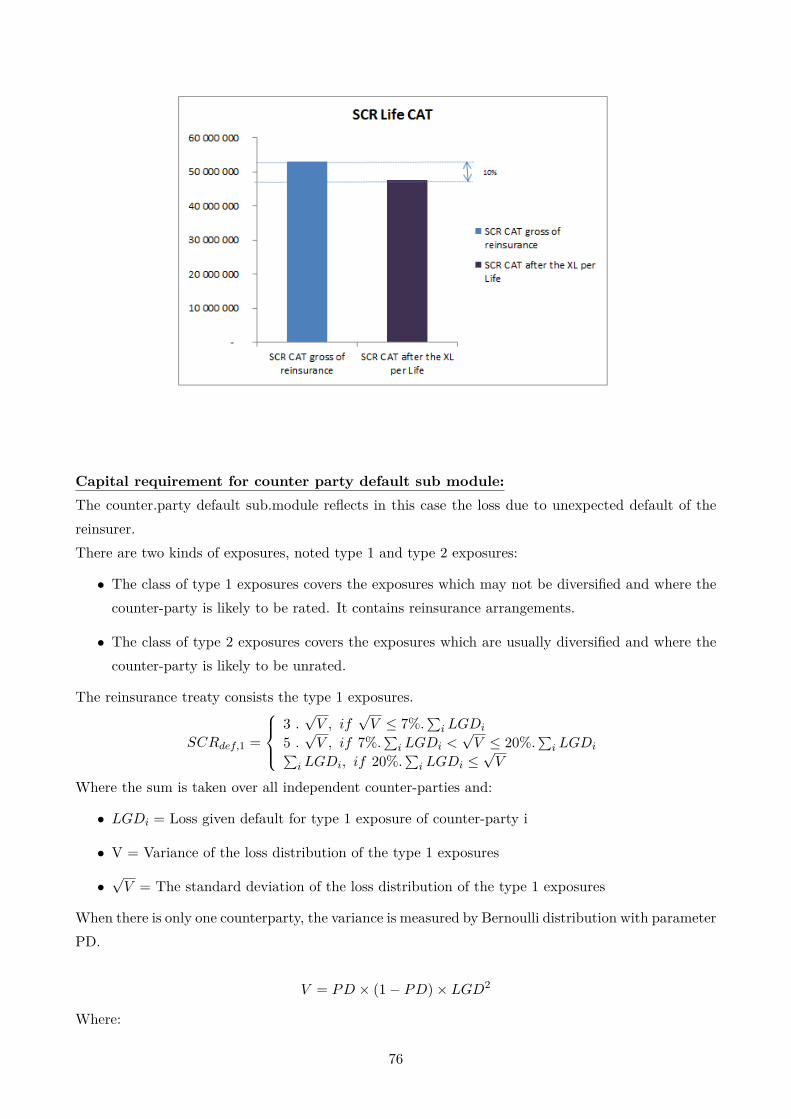
Capital requirement for counter party default sub module:The counter.party default sub.module reflects in this case the loss due to unexpected default of thereinsurer.There are two kinds of exposures, noted type 1 and type 2 exposures:
• The class of type 1 exposures covers the exposures which may not be diversified and where thecounter-party is likely to be rated. It contains reinsurance arrangements.
• The class of type 2 exposures covers the exposures which are usually diversified and where thecounter-party is likely to be unrated.
The reinsurance treaty consists the type 1 exposures.
SCRdef,1 =
3 .√V , if
√V ≤ 7%.
∑i LGDi
5 .√V , if 7%.
∑i LGDi <
√V ≤ 20%.
∑i LGDi∑
i LGDi, if 20%.∑i LGDi ≤
√V
Where the sum is taken over all independent counter-parties and:
• LGDi = Loss given default for type 1 exposure of counter-party i
• V = Variance of the loss distribution of the type 1 exposures
•√V = The standard deviation of the loss distribution of the type 1 exposures
When there is only one counterparty, the variance is measured by Bernoulli distribution with parameterPD.
V = PD × (1− PD)× LGD2
Where:
76

• PD is the probability of default
• LGD is the loss-given-default of the counterparty
The value of PD is given by credit quality steps:
The equivalent ratings are evaluated by ESMA as following:
The Solvency Capital Requirement technical specification indicated other cases where credit steps arenot available and also when the reinsurance treaty is under pooling risk concept. For the sake ofsimplification, we suppose that reinsurer has a credit quality step 2 and therefore the probability ofdefault is 0.05%. We assume that the insurer has only one reinsurer which covers both XL per Lifeand XL CAT treaty.When there is only one single name exposure, the variance is calculated as following:
V = PD.(1− PD).LGD2
For a reinsurance arrangement i , the loss.given.default should be calculated as follows:
LGDi = max(0, 50%(Recoverablesi + 50%RMre,i) + F.Collaterali)
where:
• Recoverablesi is Best Estimate recoverables from reinsurance contract i
• RMre,i is risk mitigating effect on underwriting risk of the reinsurance arrangement
77

• Collaterali is Risk-adjusted value of collateral
• F is the factor to take into account the economic effect of the collateral
For the sake of simplification, we suppose that Collateral factor is null.The risk mitigating effect RMre,i is an approximation of the difference between the (hypothetical)capital requirement for underwriting risk under the condition that the reinsurance arrangement is nottaken into account in its calculation and the capital requirement for underwriting risk (without anyamendments) (ref. [4])
RMre,i = SCRUW.gross.of.reins. − SCRUW.net.of.reins.
The calculation of RMre,i requires the complete calculation of SCR Life Underwriting on the completeportfolio. For the sake of simplification, we assume that the given example represents the wholeportfolio, there is no other risk to be consider in the module SCR Underwriting.The matrix of correlation could be applied to calculate the SCR Life Underwriting:
We assume that SCR lapse, longevity, expense and revision are null, the only sub-modules to beconsidered are mortality and CAT. In this case:
SCRLife.UW =√SCR2
mortality + 2.ρ.SCRmortality.SCRLife.CAT + SCR2Life.CAT
where ρ is correlation between sub-module mortality and sub-module CAT: 0.25
78

The recoverable best estimate is calculated based on the qx Best Estimate insurance shown in thesection 2.1.3.3 (Incident rate pricing approach) which is used in reinsurance pricing basis.The calculation of SCRdef is shown in the following table:
The final step consists of the application of the correlation matrice in order to have the total SCR:
For the sake of simplification, we assume that the total SCR consists only Life risk and counterpartyrisk. Finally,
79
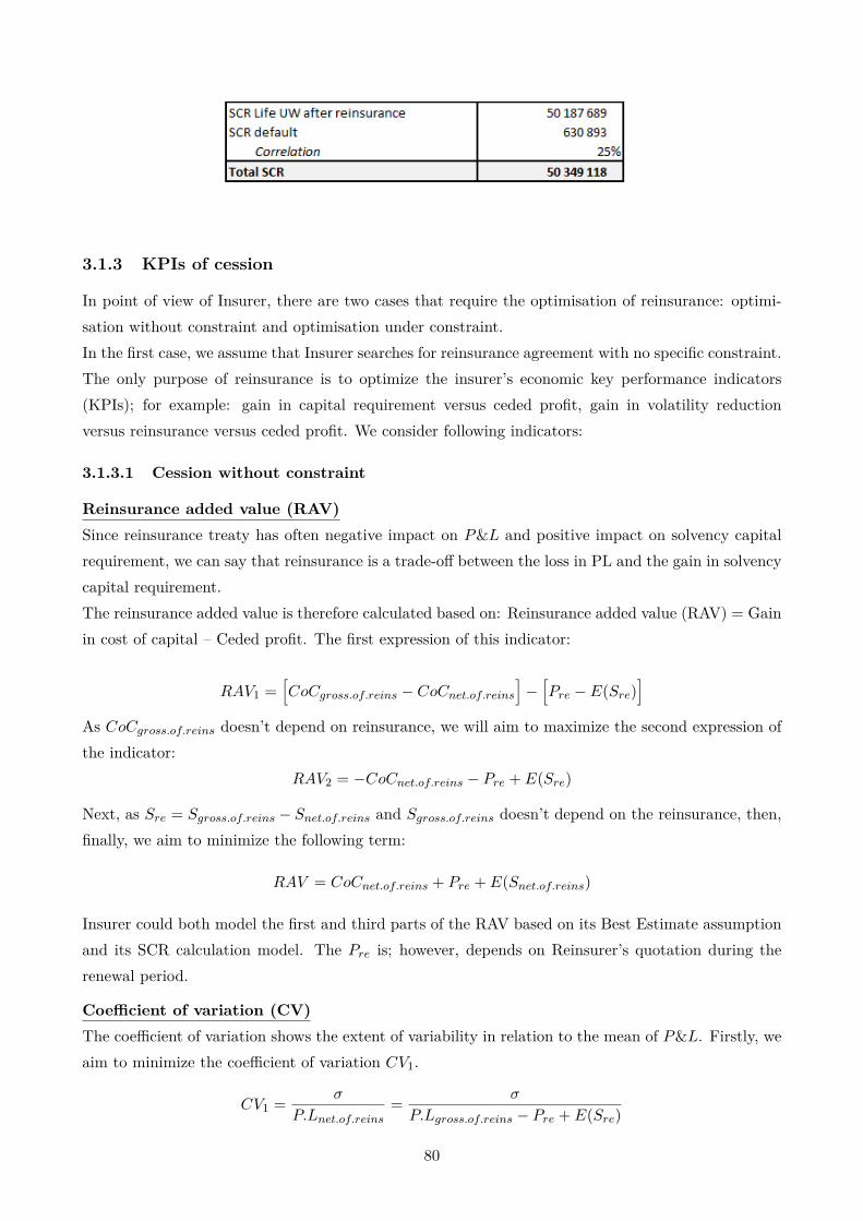
3.1.3 KPIs of cession
In point of view of Insurer, there are two cases that require the optimisation of reinsurance: optimi-sation without constraint and optimisation under constraint.In the first case, we assume that Insurer searches for reinsurance agreement with no specific constraint.The only purpose of reinsurance is to optimize the insurer’s economic key performance indicators(KPIs); for example: gain in capital requirement versus ceded profit, gain in volatility reductionversus reinsurance versus ceded profit. We consider following indicators:
3.1.3.1 Cession without constraint
Reinsurance added value (RAV)Since reinsurance treaty has often negative impact on P&L and positive impact on solvency capitalrequirement, we can say that reinsurance is a trade-off between the loss in PL and the gain in solvencycapital requirement.The reinsurance added value is therefore calculated based on: Reinsurance added value (RAV) = Gainin cost of capital – Ceded profit. The first expression of this indicator:
RAV1 =[CoCgross.of.reins − CoCnet.of.reins
]−[Pre − E(Sre)
]As CoCgross.of.reins doesn’t depend on reinsurance, we will aim to maximize the second expression ofthe indicator:
RAV2 = −CoCnet.of.reins − Pre + E(Sre)
Next, as Sre = Sgross.of.reins − Snet.of.reins and Sgross.of.reins doesn’t depend on the reinsurance, then,finally, we aim to minimize the following term:
RAV = CoCnet.of.reins + Pre + E(Snet.of.reins)
Insurer could both model the first and third parts of the RAV based on its Best Estimate assumptionand its SCR calculation model. The Pre is; however, depends on Reinsurer’s quotation during therenewal period.
Coefficient of variation (CV)The coefficient of variation shows the extent of variability in relation to the mean of P&L. Firstly, weaim to minimize the coefficient of variation CV1.
CV1 = σ
P.Lnet.of.reins= σ
P.Lgross.of.reins − Pre + E(Sre)
80

Then, as P.Lgross.of.reins doesn’t depend on reinsurance. Sre = Sgross.of.reins − Snet.of.reins andSgross.of.reins doesn’t depend on the reinsurance. Finally, we will aim to maximize following term:
CV = σ
Pre + E(Snet.of.reins)
Insurer could both model the σ and Snet.of.reins based on its own Best Estimate mortality.However, as mentioned, P re depends on Reinsurer feedback during the renewal period.
3.1.3.2 Cession with constraints
Insurer could look for reinsurance with various purposes. We will study following examples:
• (1): The reinsurer looks for a reduction of 10% of its cost of capital.
• (2): The reinsurer looks for ceding 20% of its volatility
We limit our scope of study in the optimisation with constraint.(1) Ceding 10% of the Cost of Capital:Similarly to the calculation in the sub-section 3.1.2, we calculate the cost of capital for the list ofretentions from 0 to the maximum SAR (6M) with the steps of 500K and by taking 8% as the cost ofcapital rate, we obtain following result in terms of cost of capital:
Figure 3.3: Cost of capital net of reinsurance
Figure 3.4: Cost of capital reduction after the reinsurance
The result shows that the most suitable retention is 1M.In general, the insurance should place the offer of reinsurance program with 1M retention in the marketand look for the lowest premium.
(2) Ceding 20% of the volatility:
81

We model the volatility of claim amount net of reinsurance by using Best Estimate rate:
V ar(S) =∑i
qxi .(1− qxi).Ni.SARi2
Where S: annual amount of claims net of reinsurance. SARi is the average Sum At Risk amount netof reinsurance of range i.
Figure 3.5: Standard deviation of net claim amount
Figure 3.6: Volatility reduction after reinsurance
The result suggests that the suitable level of retention according to insurers need in this case is between1.5M and 2M.
3.2 Retention and limit of XL CAT
As described in the previous part, the XL CAT treaty can not help to reduce the SCR. In fact, ingeneral, the main purpose of XL CAT reinsurance is to protect the portfolio against the catastrophicevents with extreme losses.
The limit of CAT treaty should be normally set to cover the Probable Maximum Loss in one singleevent. The PML requests a specific study based on the real exposure of insured portfolio on some veryconcentrated site: building, working factory, etc. and also eventually geological studies, etc. This isnot the purpose of this report and therefore we will just mention about it here without further details.
The retention of CAT treaty should correspond to the maximum loss that the insurance company cansustain in one single event. Each insurance company should define in their risk appetite for one singleCAT event. The risk appetite framework of insurance company is also not the scope of our study.
82
Conclusion
The proposed risk-costing or pricing models for reinsurance treaties could help the internal reinsurerto challenge reinsurer’s prices and define the best practice in terms of cession in a big insurance group.Due to the nature of data in reinsurance, it doesn’t exist an unique model which fits all cases.
For XL per life, the reinsurer could apply a frequency-severity calibration model purely based onclaim data when there is sufficient claim data. Even when the treaty is not working, this model canbe always used if reinsurer can obtain the claim data below the retention. This thesis proposes abetter quality of fit given by truncated distributions compared to usual distributions. When havingless claim data, the reinsurer could use alternative methods such as Burning Cost or incident rate or acombined method. The combined method helps to use both view in Best Estimate of insurance claimsand historical reinsured claim data.
For XL per event (CAT treaty), Generalized Pareto Distribution is often used for the calibrationof CAT risks. However, it’s interesting to test the quality of fits with other truncated "fat tail"distributions. The past models: Strickler’s model and Erland Ekheden’s CAT model in life were basedon some strong assumption using public historical claim data in EMDAT. This report integrated alsothe terrorism claim data in GTD database. In additional, it proposes to use the portfolio Sum At Riskdistribution data in the simulation of claim amounts and also to add the geographical concentrationscenarios in the list of scenarios.
The optimization of reinsurance plays also an important role in the reinsurance management. Depend-ing on the need of insurer in terms of volatility or required capital, an optimal reinsurance programcan be defined to help insurer to obtain its objectives.
This thesis presented only a small part of life reinsurance activities. In particular, for internal reinsur-ance activities, the third important role such as capturing diversification is not studied in this thesis.Also, the modelling of proportional reinsurance is not mentioned. In general, with the implementa-tion of solvency II with the requirement of better managing the risk and with the new age of data,reinsurance will have no doubt big advantage in not only risk management but also insurance business.
83

Appendix A
Example: calculation of Cost of capitalin Burning Cost pricing
We suppose that Reinsurer follows standard formula. Reinsurer firstly calculates its SCR Life UWcontaining mainly SCR CAT and SCR mortality based on the sum at risk and the standard formulashock. The total SCR attached to the reinsurance treaty is calculated by the SCR Life UW times atransmission factor.
The calculation is performed in the following table:
In practice, the qx is calibrated depending on each reinsurer. The qx taken in this example is basedon the local entity view of the risk (based on qx Best Estimate).
84

Bibliography
[1] John E.Tiller, Denise Fagerberg Tiller. Life, Health Annuity Reinsurance. Fourth Edition,2015.
[2] Erland Ekheden. [Mathematical Statistics - Stockholm University]. The Pricing of CatastropheCover In Life Reinsurance, 2008.
[3] Alexandra Field. [RGA International]. The future of (Life) Reinsurance Evolution or Rev-olution?, 2015.
[4] EIOPA. [European Insurance and Occupation Pensions Authority]. Technical Specification forthe Preparatory Phase - Part I , 2014.
[5] Fritz Scholz. [Stat 498B Industrial Statistics]. Inference for the Weibull Distribution, 2008.
[6] Committee of European Banking Supervisor. Standardised Approach: Mapping of ECAIs’credit assessments to credit quality steps.
85