Multiple Scattering

θ0

Lx0

When protons pass through a slab of material they suffer millions of collisions with

atomic nuclei. The statistical outcome is a multiple scattering angle whose distribution is

approximately Gaussian. For protons, this angle is always small so the projected

displacement in any measuring plane MP is also Gaussian. The width parameter of the

angular distribution is θ0 . The corresponding displacement, x0 , can easily be measured

by scanning a dosimeter across the MP. The task of multiple scattering theory is to

predict θ0 given the scattering material and thickness, and the incident proton energy.

MP

Many statistical processes obey the Central Limit Theorem: the random sum of

many small displacements is a Gaussian distribution. However, the displacements

must all be small , in a sense that can be made mathematically precise. Scattering

from the screened Coulomb field of the atomic nucleus does not obey the CLT

because the single scattering cross section falls off only as 1/θ4 , too slowly.

Therefore the angular distribution is approximately Gaussian for small angles but

eventually tends to a ‘single scattering tail’ ≈ 1/θ4 .

All this was well understood by many investigators who worked on multiple

scattering in the 1920’s and 30’s but it was Molière who in 1947 published the

definitive theory, uniting the Gaussian region with the large-angle region in a

precise and elegant way. He computed the distributions of both the space and

projected angles for arbitrarily thick targets as well as compounds and mixtures, and

produced numerical results long before the general availability of digital computers.

His numerical evaluations were later improved somewhat by Bethe, who

considered the overall Molière theory to be good to 1%.

His name notwithstanding, Molière was German. In his first paper, he derives an

accurate formula for single scattering in the screened Coulomb field of the nucleus.

The second, which uses that formula to compute multiple scattering, was his

‘Habilitationsschrift’ (a published work that qualified one to join the faculty) at the

University of Tübingen. He thanks Prof. Heisenberg for his interest and advice.

Molière Theory

Hanson et al., ‘Measurement of

multiple scattering of 15.7 MeV

electrons,’ Phys. Rev. 84 (1951)

634-637 studied electron

scattering by thin and thick foils

of Be and Au. They also gave a

formula for computing the

width of the best Gaussian fit

to the exact theory (‘Hanson’s

formula’ below). Their overall

measurements agree well with

Molière not only in the small

angle (Gaussian) region but also

in the single scattering tail. The

theoretical transition between

the two regions was improved

by Bethe later on.

An Early Measurement with Electrons

place

H. Bichsel, ‘Multiple scattering

of protons,’ Phys. Rev. 112

(1958) 182-185 bombarded

targets of Al, Ni, Ag and Au

with protons ranging from 0.77

to 4.8 MeV from a Van de

Graaff accelerator. His detector

was a tilted nuclear track plate.

He fitted his measurements

with the Molière form at the

appropriate B, adjusting only

the characteristic angle θ0 . The

results agreed with theory to

±5%. Bichsel went on to

become a leading expert in

range-energy and straggling

theory and modeling the Bragg

peak.

The First Measurement with Protons

Gottschalk et al., ‘Multiple

Coulomb scattering of 160

MeV protons,’ Nucl. Instr.

Meth. B74 (1993) 467-490.

Molière theory predicts the

multiple scattering angle

correctly over the periodic

table, three decades of

normalized target thickness

and over two decades of

angle. Compounds and

mixtures (not shown) are

also covered. The theory has

no empirical parameters!

Comprehensive Test of Molière Theory

Although Molière starts his paper by considering thin elementary targets,

presumably for clarity, he later covers thick scatterers as well as

compounds and mixtures. Both generalizations are very important for

proton beam line design and dose algorithms. Early workers in the field,

such as Bichsel and Scott, were well aware of these generalizations.

However, Bethe’s 1953 paper (in English) didn’t include those aspects. His

remark ‘Lewis5 has shown how the energy loss can be taken into account

...’ seems odd because Molière also shows it. In any event, Bethe was

interested in other aspects of the theory, and made a number of

improvements.

Some English-speaking readers apparently thought Bethe’s review was

comprehensive and assumed that Molière theory only applied when the

energy loss was small. ‘Effective energy’ fixes were used. Molière’s original

papers were always cited, of course!

‘But it’s in German!’

This paper by two

well-known theorists

manages to make

two mistakes in the

same paragraph.

Molière theory does

cover energy loss,

and if a single

kinematic factor is

used in simpler

theories, it should be

the geometric not the

arithmetic mean of

the incoming and

outgoing values.

Caveat Emptor

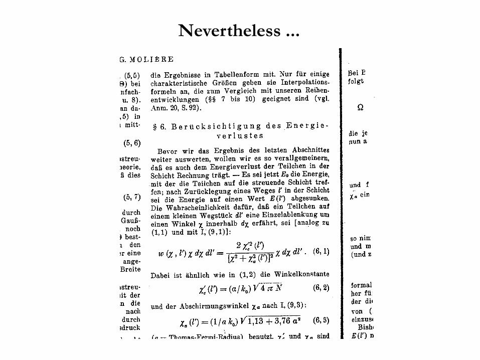
Nevertheless ...

Physical Interpretation of B

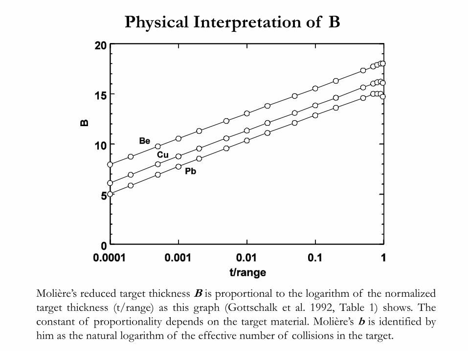
Molière’s reduced target thickness B is proportional to the logarithm of the normalized

target thickness (t/range) as this graph (Gottschalk et al. 1992, Table 1) shows. The

constant of proportionality depends on the target material. Molière’s b is identified by

him as the natural logarithm of the effective number of collisions in the target.

The Gaussian Approximation

This simple formula circumvents the Molière calculation and is often used as a

proxy for Molière theory in the Gaussian approximation. The scattering material is

entirely represented by its radiation length LR , which we can look up or calculate

from the chemical composition. Highland’s formula may be generalized to thick

targets by integration but we must take the correction factor [ ] outside the integral.

In Molière theory we first find, by a lengthy computation, a single scattering

parameter χC and a dimensionless target thickness parameter B. The quantity χC√B,

a characteristic multiple scattering angle, is the scale factor in a PDF which consists

of three terms in powers of 1/B . The first is a Gaussian.

Hanson et al. (Phys. Rev. 84 (1951) 634) were the first to observe that the best

Gaussian approximation is obtained, not by retaining just Molière’s first term, but

by using a Gaussian whose σ is a bit narrower, θ0 = χC√(B-1.2) . This approach still

requires the entire Molière computation.

Later, V.L. Highland (NIM 129 (1975) 497-499) fitted Molière/Bethe/Hanson

theory and found

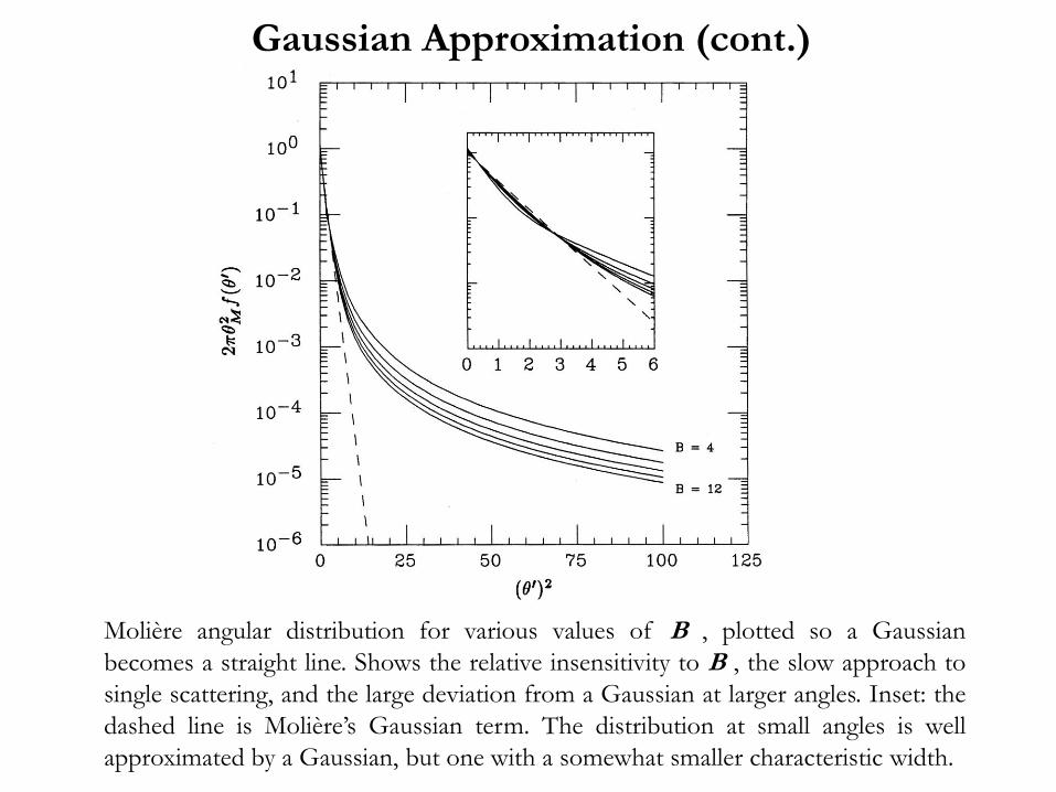
Molière angular distribution for various values of B , plotted so a Gaussian

becomes a straight line. Shows the relative insensitivity to B , the slow approach to

single scattering, and the large deviation from a Gaussian at larger angles. Inset: the

dashed line is Molière’s Gaussian term. The distribution at small angles is well

approximated by a Gaussian, but one with a somewhat smaller characteristic width.

Gaussian Approximation (cont.)

0

10

20

30

40

50

60

70

-30 -20 -10 -0 10 20 300.0001

0.001

0.01

0.1

1

10

100

mrad

Moliere

2.5 (99%)

Hanson, Highland

mrad

mrad

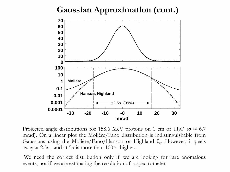
Gaussian Approximation (cont.)

Projected angle distributions for 158.6 MeV protons on 1 cm of H2O (σ ≈ 6.7mrad). On a linear plot the Molière/Fano distribution is indistinguishable fromGaussians using the Molière/Fano/Hanson or Highland θ0. However, it peelsaway at 2.5σ , and at 5σ is more than 100× higher.

We need the correct distribution only if we are looking for rare anomalousevents, not if we are estimating the resolution of a spectrometer.

Same paper as before, but measurements are fit with a Gaussian. We

regard Molière/Fano/Hanson as the gold standard in the Gaussian

approximation, and will try to construct a scattering power which,

when integrated over target thickness, will reproduce it.

Molière/Fano/Hanson (θHanson)

Generalized Highland (θHighland)

Same data, Gaussian fit. Agreement of this simple formula is almost as

good as θHanson (full calculation). (Be is slightly high because Highland

fitted Molière/Bethe/Hanson instead of Molière/Fano/Hanson.)

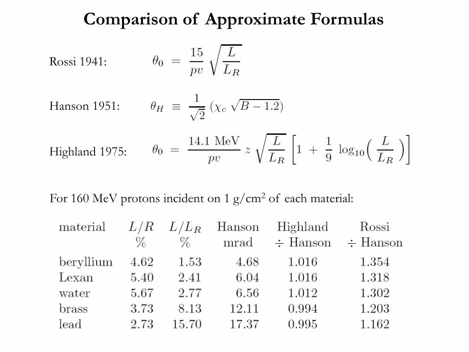
Hanson 1951:

Rossi 1941:

Highland 1975:

For 160 MeV protons incident on 1 g/cm2 of each material:

Comparison of Approximate Formulas

Highland’s Formula for Thick Targets

Unlike the full Molière theory, Highland’s formula as originally given applies only

to thin targets, as shown by the telltale factor pv. We extended it to moderately

thick and very thick targets. In the first case it is frequently good enough to

replace pv by its geometric mean : pv → p1v1p2v2 where 1,2 refer to the incoming

and outgoing proton. For very thick targets, however, it is necessary to integrate

over the target thickness, assuming, of course, that the proton range-energy

relation is known.

Notice that we have taken the logarithmic correction factor out of the integral. It is

evaluated for the target as a whole. Without this step (if we think of evaluating the

integral numerically) the answer would get ever smaller as dt′ became smaller.

Other arbitrary measures could be used, such as fixing the integral step size. This

is the one we prefer, and the one used in comparing Highland’s formula with data

in our paper.

Because of the way the integrand depends on depth, it is efficient to divide the

target by equal ratios rather than equal steps when evaluating the integral

numerically.

This shows the accuracy of Highland’s formula, as generalized to thick targets by

us., as a parameterization of Hanson’s formula applied to the Bethe form of

Molière theory. It is good to ±5% as claimed by Highland except for the thinnest

points for lead, which are outside his allowed range.

Accuracy of Highland’s Formula

A well collimated beam of protons scattered in the target and fell on a measuring

plane where the transverse dose distribution was measured by a diode. The data

were fit to obtain θM and θ0 and the corresponding ‘air’ (target out) angle was

subtracted in quadrature. In converting to angle, the virtual source position was

obtained from theory. Over 20 years, 115 different thicknesses and materials were

measured with steadily more automated methods but the same basic principle.

The HCL Experiment 1967-1987

Top: air run and thin through thick Be runs. Bottom: air run an thin through thick Pb

runs. Top right each frame: normalized target thickness. Main frame: measured data in

a semilog plot. Bottom window each frame: fit residual in a linear ±5% window.

Typical Data and Fits

Because of the rather short throw in the HCL experiment (to conserve signal), it was

necessary, especially for the thicker targets, to estimate where the protons were coming

from. We called this the ‘effective origin’ of scattered particles. The proper term per

ICRU Report 35 (1984) is ‘virtual point source’. The diagram suggests how it may be

calculated. First, we need an expression for the size parameter of the scattered beam

as a function of z. Then we extrapolate from two sufficiently distant points. Details

may be found in the paper and will be covered in a later lecture.

The Virtual Point Source

This graph shows the sweep of Molière theory. With no empirical parameters it

predicts the characteristic multiple scattering angle from Be to Pb over three

decades of normalized target thickness and two decades of multiple scattering

angle.

Overview of HCL Results

At the Bragg peak, because of range straggling, there is no longer any strong correlation

between depth and proton energy, and the multiple scattering angle appears to saturate.

Behavior Near End-of-Range

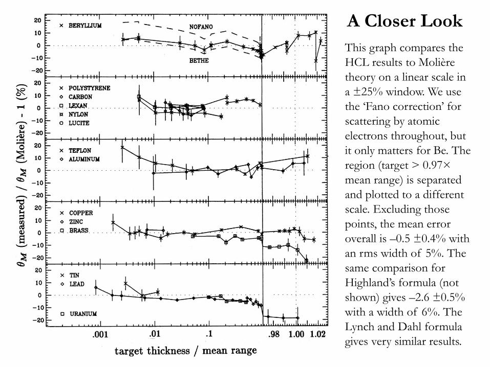
This graph compares the

HCL results to Molière

theory on a linear scale in

a ±25% window. We use

the ‘Fano correction’ for

scattering by atomic

electrons throughout, but

it only matters for Be. The

region (target > 0.97×

mean range) is separated

and plotted to a different

scale. Excluding those

points, the mean error

overall is –0.5 ±0.4% with

an rms width of 5%. The

same comparison for

Highland’s formula (not

shown) gives –2.6 ±0.5%

with a width of 6%. The

Lynch and Dahl formula

gives very similar results.

A Closer Look

We reviewed and in some cases reanalyzed the six previous proton studies. Some of

those claimed Molière’s theory was wrong, others were not aware of his generalization

to thick targets. The summary, above, is plotted to an arbitrary abscissa with each

experiment averaged over everything but target material. The experiments ranged from

1 MeV to 200 GeV. The mean is –0.3 ±0.5% (!) with an rms spread of 3%.

Grand Summary

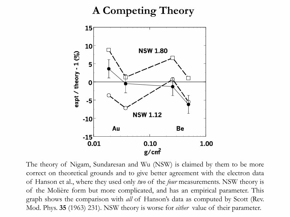
The theory of Nigam, Sundaresan and Wu (NSW) is claimed by them to be more

correct on theoretical grounds and to give better agreement with the electron data

of Hanson et al., where they used only two of the four measurements. NSW theory is

of the Molière form but more complicated, and has an empirical parameter. This

graph shows the comparison with all of Hanson’s data as computed by Scott (Rev.

Mod. Phys. 35 (1963) 231). NSW theory is worse for either value of their parameter.

A Competing Theory

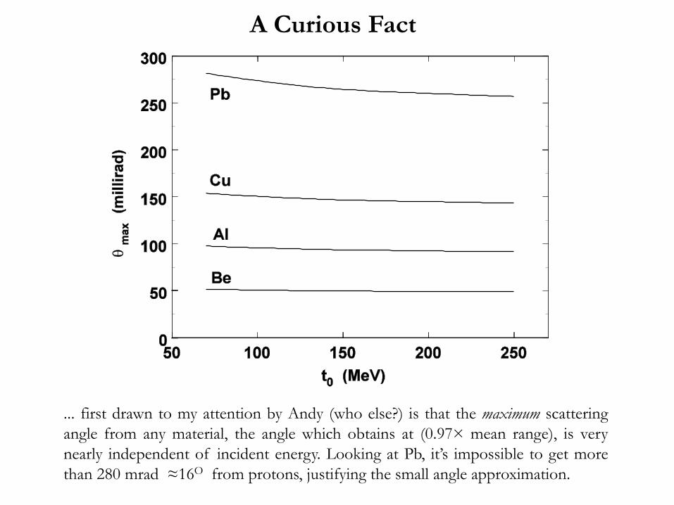
... first drawn to my attention by Andy (who else?) is that the maximum scattering

angle from any material, the angle which obtains at (0.97× mean range), is very

nearly independent of incident energy. Looking at Pb, it’s impossible to get more

than 280 mrad ≈16O from protons, justifying the small angle approximation.

A Curious Fact

That this procedure is, strictly speaking, incorrect is easily seen. Divide a scatterer

made of a single material into halves. Their quadratic sum will always be too small

by ~3%, as can also be seen directly from Highland’s formula. The error is worse,

the more you divide the scatterer.

Nevertheless, addition in quadrature works well enough in practice, perhaps

because in common engineering situations one of the slabs will dominate.

A better method suggested by Lynch and Dahl (Nucl. Instr. Meth. B58 (1991) 6-

10) is not practical for beam line design, essentially because it does not allow us to

compute slabs separately. The entire issue of mixed slabs is rather complicated, and

will be covered later.

Combining

ScatterersIn beam line design we frequently need to compute the net multiple scattering angle

from (say) a sheet of plastic followed by a sheet of lead, or some even more

complicated set of ‘homogeneous slabs’.

Molière theory does not apply to a sheet of plastic followed by a sheet of lead. (It

would apply to a fine mixture of plastic and lead!) However, we can find each

characteristic angle by itself (taking energy loss into account) and add them in

quadrature:

Summary

The Molière theory of multiple scattering applies to compounds and mixtures,and target thicknesses up to ~97% of the mean range. It has no adjustableparameters. It is at least accurate as available experiments (a few percent).

Highland’s approximation to the characteristic angle of the best Gaussian fit isnearly as good as Hanson’s formula based on the full theory, and far easier toevaluate. For thick targets, it must be integrated. For targets of intermediatethickness one can replace pv by (p1v1p2v2)

1/2.

In beam line design, finite slabs can be combined to sufficient accuracy by addingtheir characteristic angles in quadrature.

High-Z materials (lead) scatter far more than low-Z materials (water, plastic). Wewill make use of this to design contoured scatterers compensated for energy lossor range modulators compensated for scattering angle.