Remote Sensing of Environment 140 (2014) 78–93

Contents lists available at ScienceDirect

Remote Sensing of Environment

j ourna l homepage: www.e lsev ie r .com/ locate / rse

Remote sensing of diffuse attenuation coefficient usingMODIS imagery ofturbid coastal waters: A case study in Bohai Sea

Jun Chen a,b,⁎, Tingwei Cui c, Junwu Tang d, Qingjun Song e

a School of Ocean Sciences, China University of Geosciences, Beijing 100083, Chinab Key Laboratory of Marine Hydrocarbon Resources and Environmental Geology, Qingdao Institute of Marine Geology, Qingdao 266071, Chinac First Institute of Oceanography, State Oceanic Administration, Qingdao 266071, Chinad National Ocean Technology Center, Tianjin 300111, Chinae National Satellite Ocean Application Service, Beijing 100081, China

Corresponding author at: No.29, Xueyuan Road, BeijE-mail address: cjun@cgs.cn (J. Chen).

0034-4257/$ – see front matter © 2013 Elsevier Inc. All rihttp://dx.doi.org/10.1016/j.rse.2013.08.031

a b s t r a c t

a r t i c l e i n f o

Article history:Received 2 March 2013Received in revised form 22 August 2013Accepted 22 August 2013Available online xxxx

Keywords:Remote sensingDiffuse attenuationMODISBohai Sea

The objectives of this study are to evaluate the applicability of three existing retrieval algorithms of diffuse atten-uation coefficients of downwelling irradiance at 490 nm, Kd(490), for turbid Case II waters, and to improve theseexisting models using a simple semi-analytical (SSA) model. In this study, based on comparison of the Kd(490)predicted by these models with field measurements taken in the Bohai Sea and Yellow Sea, it is shown thatthe SSA model provides a stronger performance than these three selected existing models. The atmospheric in-fluences on the MODIS data are removed using an improved shortwave infrared band-based (ISWIR-based)model, which is capable of retrieving spectral remote sensing reflectance within 19% uncertainty. The Kd(490)data was quantified from the MODIS images after atmospheric correction using the SSA model and Wang'smodel. The study results indicate that the SSA model produces 31.51% uncertainty in deriving Kd(490) fromMODIS data, which is 12.1% higher than Wang's model. This study demonstrates the potential of the SSAmodel in estimating Kd(490) even in highly turbid coastal waters.

© 2013 Elsevier Inc. All rights reserved.

1. Introduction

The light available in the water column at wavelength ranges from400 to 700 nm in the visible parts of the spectrum (Bukata, Jerome,Kondratyev, & Pozdnyakov, 1995) is referred to as photosyntheticallyactive radiation (PAR). It is a natural component of irradiance reachingthe Earth's surface, and its potential to influence ecological processesand biogeochemical cycles in natural waters has long been recognized(Robert, Alexander, & Kirill, 1995). In aquatic environments, this lightlimits the growth of phytoplankton, and is a first order determinant ofthe response of phytoplankton to nutrient input in the sea. In otherwords, the PAR is used by phytoplankton for photosynthesis andconstrains the type and distribution of algae species and benthic algae,thus contributing significantly to total primary production (Carter,Ross, Schiel, Howard-Williams, & Hayden, 2005). From the perspectiveof an energy cycle, the supply of PAR for phytoplankton growth inaquatic environments is a product of the input of solar radiation atthe surface. The PAR supply is reduced by optically active constitu-ents through absorption and scattering, which are increased byhigher phytoplankton concentrations (Devlin et al., 2009). There-fore, light, together with nutrients, is a major governing parametercontrolling production and photosynthetic processes in aquatic en-

ing, China.

v-i- ⁎

ghts reserved.

ronments (Lund-Hansen, 2004). Furthermore, the estimation oflight diffuse attenuation coefficients, Kd(λ), in an aquatic environ-ment, is a critical factor to understand physical processes such asheat transfer in the upper layer of the ocean (Wu, Sathyendranath,& Platt, 2007).

Although capable of providing accurate measurements, traditionalfield monitoring on spatial distribution of Kd(λ) is costly and time con-suming, and thus confounds in coastal and oceanic systems by hightemporal and spatial variability (Sweeney, Titterton, & Leonard, 1991).Recent advances in optical sensor technology have opened new oppor-tunities to study biogeochemical processes in aquatic environments atspatial and temporal scales which previously had not been possible(Clavano, Boss, & Lee, 2007). These advances have allowed scientiststo utilize ocean color satellite images to synoptically investigate large-scale surface features in the world's oceans (Chang & Gould, 2006). Forexample, since the launch of the Coastal Zone Color Scanner (CZCS) in1978, the ocean-color community has provided maps of Kd(λ) at largespatial scales, offering a great improvement in spatial and temporalresolution compared to in situ data (Barale, 1987). More recently, thelaunch of the Sea-viewing Wide Field-of-view Sensor (SeaWiFS) onSeptember 18, 1997 has allowed the global ocean color data to be avail-able to the science community in near-real time (Mueller & Trees, 1997).SeaWiFS was on a sun-synchronous satellite with a 2801 km swathwidth, providing 2-day coverage of the global ocean with a nadir resolu-tion of ~1 km per pixel (Mueller & Fargion, 2002). Shortly afterwards,

79J. Chen et al. / Remote Sensing of Environment 140 (2014) 78–93

two Moderate Resolution Imaging Spectroradiometers (MODIS) werelaunched by NASA on 1999 and 2002, respectively. These satellite sen-sors provided near-daily coverage of the global ocean. The study resultsobtained by Gordon and Voss (1999) indicated thatMODISwas typically2–3 timesmore sensitive than SeaWiFS, which in turnwas approximate-ly twice as sensitive as CZCS.

Traditionally, the in situ spectral Kd(λ) had been measured by theocean-color scientific community at 490 nm, following the primarystudies performed in the 1970s (Smith & Baker, 1978). These achieve-ments had a great impact on our knowledge of the world's oceans.Shortly afterwards, Austin and Petzold (1981) found an empirical re-lationship between CZCS observations and the diffuse attenuationcoefficient for green light at 490 nm. Stumpf and Pennock (1991)used solutions obtained using the radiative transfer equation to de-rive relationships of water reflectance to Kd(λ) in moderately turbidwaters (0.5 m−1 b Kd(490) b 5 m−1). Datasets collected from theNational Oceanic and Atmospheric Administration (NOAA) AdvancedVery High Resolution Radiometer (AVHRR) and field measurementsobtained from Delaware Bay showed that the values of Kd(490) calcu-lated from the reflectance data agreed to within 60% of the observedvalues. However, due to limitations in the capabilities of the sensorand the atmospheric corrections, the results of these studies are suitableonly for waters having an attenuation coefficient of less than 0.5 m−1

and a predominance of absorbing material (Siegel & Dickey, 1987). Atpresent, the standard method (Mueller's model) to estimate values ofKd(490) from remotely sensed data is through empirical relationshipsbetween Kd(490) and the spectral ratio of water-leaving radiance attwo wavelengths (Mueller & Trees, 1997). Such a model is insufficientto provide an understanding of the variation of Kd(490), and involveslarge uncertainties inherent to empirical models (Lee, Du, & Arnone,2005). In order to overcome these limitations, several empiricaland semi-analytical models of Kd(490) are developed for retrievingKd(490) maps from satellite data. Morel et al. (2007) proposed anempirical relationship between Kd(490) and chlorophyll-a concentra-tion (chla). However, due to the complete neglect of the influences ofsuspended sediment matters involved in the retrieval results, theseresults are only suitable for Case I waters.

In order to accurately derive Kd(490) from turbid Case II waters, Leeet al. (2005, 2007) provided a semi-analytical relationship (Lee'smodel)between Kd(490) and inherent optical properties based on the radiativetransfer equation, with values of the model parameters derived fromMonte Carlo simulations using the averaged particle phase function.The model was further tested with data simulated using significantlydifferent particle phase functions, and the model-derived Kd(490) wasfound to match the simulation results very accurately. The retrievalaccuracy of this model is greatly dependent on the performance of thequasi-analytical algorithm (QAA model) suggested by Lee, Carder, andArnone (2002). Ivey (2009) applied the QAA model to derive the re-spective bb(λ) from coastal waters of Puget Sound, Washington, Stock-ing Island, Bahamas, and West Florida Shelf, and indicated that theQAA model produces a poor performance in bb(λ) predictions, with anestimation uncertainty of N50%. Zhang, Stramski, and Reynolds (2010)also demonstrated that the QAA-derived spectral exponent of particu-late backscattering generally leads to overestimation of both backscat-tering and absorption at wavelengths shorter than 551 nm, and mayyield negative absorption coefficients in the Arctic waters as well asmany coastal locations. Therefore, due to the failure of the QAA modelin deriving inherent optical properties, Lee's model may produce poorperformance in optically complex coastal waters.

Recently,Wang, Son, andHarding (2009) proposed a Kd(490)model(referred to as Wang's model) for deriving Kd(490) from coastal turbidwaters. The model uses a relationship relating the backscattering coeffi-cient at thewavelength 490 nm to the irradiance reflectance just beneaththe surface, at the red wavelengths. Using the in situ-derived bb(490) re-lationship observed in Chesapeake Bay, Wang, Son, and Harding (2009)found that Kd(490) models were formulated using the semi-analytical

approach. Match-up comparisons between the MODIS-derived and in-situ-measured Kd(490) products observed in Chesapeake Bay indicatethat the satellite-derived data using the proposed models are well cor-related with the in situ measurements. In Wang's model, Wang, Son,and Harding (2009) related bb(490) to the irradiance reflectance justbeneath the surface at wavelength 670 nm. However, in addition tobackscattering by all particulate matter, the irradiance reflectance at670 nm is also affected by total absorption coefficient (Gordon et al.,1988; Lee et al., 2002). If the total absorption coefficient at 670 nm variesbetween samples, the bb(490) model output may be different for thesame bb(670). Thus, Wang's model may be violated in some complexcases, e.g. cases involving high chla concentrations. For the estimationof Kd(λ), which is important for studies regarding heat budgets and pho-tosynthesis (Ohlmannn, Siegel, & Mobley, 2000; Sathyendranath, Prieur,& Morel, 1989; Wu et al., 2007), a model which is capable of providinga higher level of accuracy remains desired.

The objectives of this study are to validate the respective perfor-mances of Mueller, Lee and Wang's models, and to further improvethese for turbid Case II waters using an innovative simple semi-analytical (SSA) model. The specific goals of the study are as follows:(1) to evaluate the accuracy of Mueller, Lee and Wang's models foraccurately estimating Kd(490) in turbid coastal waters; (2) to improvethe performance of Mueller, Lee and Wang's models by a proposedSSA model with the spectral bands of the MODIS sensor; and (3) tocompare the accuracy of Mueller, Lee and Wang's models, and the SSAmodel in estimating Kd(490) from highly turbid and productive coastalwaters in China.

2. Data, methods and techniques

2.1. Accuracy assessment

In this study, the Root-Mean-Square (RMS) of the ratio of modeled-to-measured values is used to assess the accuracy of atmosphericcorrection. This statistic will be referred to as RMS and is describedby the following equation (Carder, Chen, Lee, Hawes, & Cannizzaro,2003; O'Reilly et al., 1998):

REi ¼xmod;i−xobs;i

xobs;i

����������� 100% ð1Þ

RMS ¼

ffiffiffiffiffiffiffiffiffiffiffiffiffiffiffiffiXni¼1

RE2i

n−2

vuuut� 100% ð2Þ

where REi is the relative uncertainty of the ith observation, xmod,i isthe modeled value of the ith element, xobs,i is the observed value ofthe ith element, and n is the number of elements.

2.2. Study area

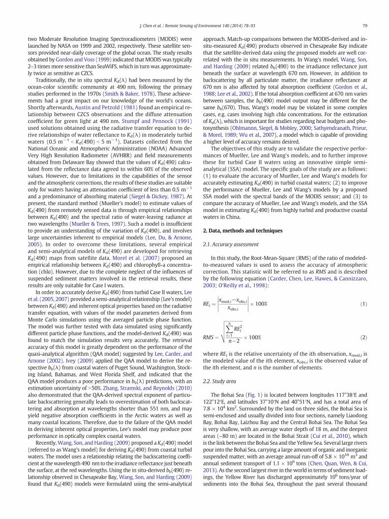
The Bohai Sea (Fig. 1) is located between longitudes 117°38′E and122°12′E, and latitudes 37°10′N and 40°51′N, and has a total area of7.8 × 104 km2. Surrounded by the land on three sides, the Bohai Sea issemi-enclosed and usually divided into four sections, namely LiaodongBay, Bohai Bay, Laizhou Bay and the Central Bohai Sea. The Bohai Seais very shallow, with an average water depth of 18 m, and the deepestareas (~80 m) are located in the Bohai Strait (Cui et al., 2010), whichis the linkbetween the Bohai Sea and the Yellow Sea. Several large riverspour into the Bohai Sea, carrying a large amount of organic and inorganicsuspended matter, with an average annual run-off of 5.8 × 1010 m3 andannual sediment transport of 1.1 × 109 tons (Chen, Quan, Wen, & Cui,2013). As the second largest river in theworld in terms of sediment load-ings, the Yellow River has discharged approximately 109 tons/year ofsediments into the Bohai Sea, throughout the past several thousand

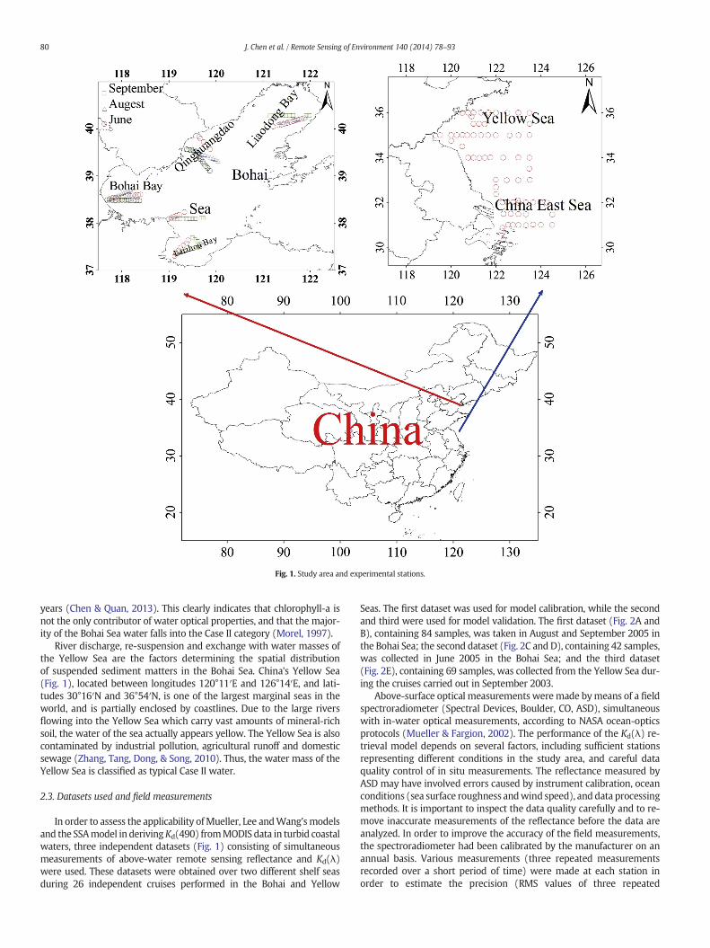
Fig. 1. Study area and experimental stations.

80 J. Chen et al. / Remote Sensing of Environment 140 (2014) 78–93

years (Chen & Quan, 2013). This clearly indicates that chlorophyll-a isnot the only contributor of water optical properties, and that the major-ity of the Bohai Sea water falls into the Case II category (Morel, 1997).

River discharge, re-suspension and exchange with water masses ofthe Yellow Sea are the factors determining the spatial distributionof suspended sediment matters in the Bohai Sea. China's Yellow Sea(Fig. 1), located between longitudes 120°11′E and 126°14′E, and lati-tudes 30°16′N and 36°54′N, is one of the largest marginal seas in theworld, and is partially enclosed by coastlines. Due to the large riversflowing into the Yellow Sea which carry vast amounts of mineral-richsoil, the water of the sea actually appears yellow. The Yellow Sea is alsocontaminated by industrial pollution, agricultural runoff and domesticsewage (Zhang, Tang, Dong, & Song, 2010). Thus, the water mass of theYellow Sea is classified as typical Case II water.

2.3. Datasets used and field measurements

In order to assess the applicability ofMueller, Lee andWang'smodelsand the SSAmodel in derivingKd(490) fromMODIS data in turbid coastalwaters, three independent datasets (Fig. 1) consisting of simultaneousmeasurements of above-water remote sensing reflectance and Kd(λ)were used. These datasets were obtained over two different shelf seasduring 26 independent cruises performed in the Bohai and Yellow

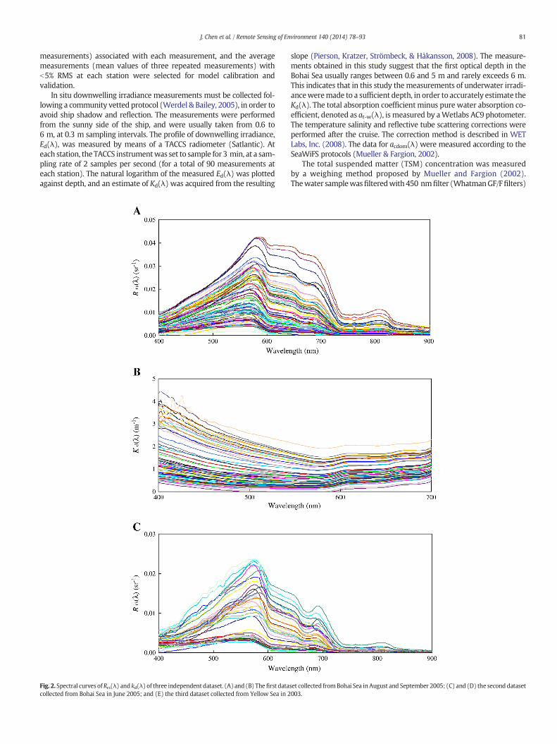
Seas. The first dataset was used for model calibration, while the secondand third were used for model validation. The first dataset (Fig. 2A andB), containing 84 samples, was taken in August and September 2005 inthe Bohai Sea; the second dataset (Fig. 2C and D), containing 42 samples,was collected in June 2005 in the Bohai Sea; and the third dataset(Fig. 2E), containing 69 samples, was collected from the Yellow Sea dur-ing the cruises carried out in September 2003.

Above-surface optical measurements weremade bymeans of a fieldspectroradiometer (Spectral Devices, Boulder, CO, ASD), simultaneouswith in-water optical measurements, according to NASA ocean-opticsprotocols (Mueller & Fargion, 2002). The performance of the Kd(λ) re-trieval model depends on several factors, including sufficient stationsrepresenting different conditions in the study area, and careful dataquality control of in situ measurements. The reflectance measured byASD may have involved errors caused by instrument calibration, oceanconditions (sea surface roughness andwind speed), and data processingmethods. It is important to inspect the data quality carefully and to re-move inaccurate measurements of the reflectance before the data areanalyzed. In order to improve the accuracy of the field measurements,the spectroradiometer had been calibrated by the manufacturer on anannual basis. Various measurements (three repeated measurementsrecorded over a short period of time) were made at each station inorder to estimate the precision (RMS values of three repeated

81J. Chen et al. / Remote Sensing of Environment 140 (2014) 78–93

measurements) associated with each measurement, and the averagemeasurements (mean values of three repeated measurements) withb5% RMS at each station were selected for model calibration andvalidation.

In situ downwelling irradiance measurements must be collected fol-lowing a community vetted protocol (Werdel & Bailey, 2005), in order toavoid ship shadow and reflection. The measurements were performedfrom the sunny side of the ship, and were usually taken from 0.6 to6 m, at 0.3 m sampling intervals. The profile of downwelling irradiance,Ed(λ), was measured by means of a TACCS radiometer (Satlantic). Ateach station, the TACCS instrumentwas set to sample for 3 min, at a sam-pling rate of 2 samples per second (for a total of 90 measurements ateach station). The natural logarithm of the measured Ed(λ) was plottedagainst depth, and an estimate of Kd(λ) was acquired from the resulting

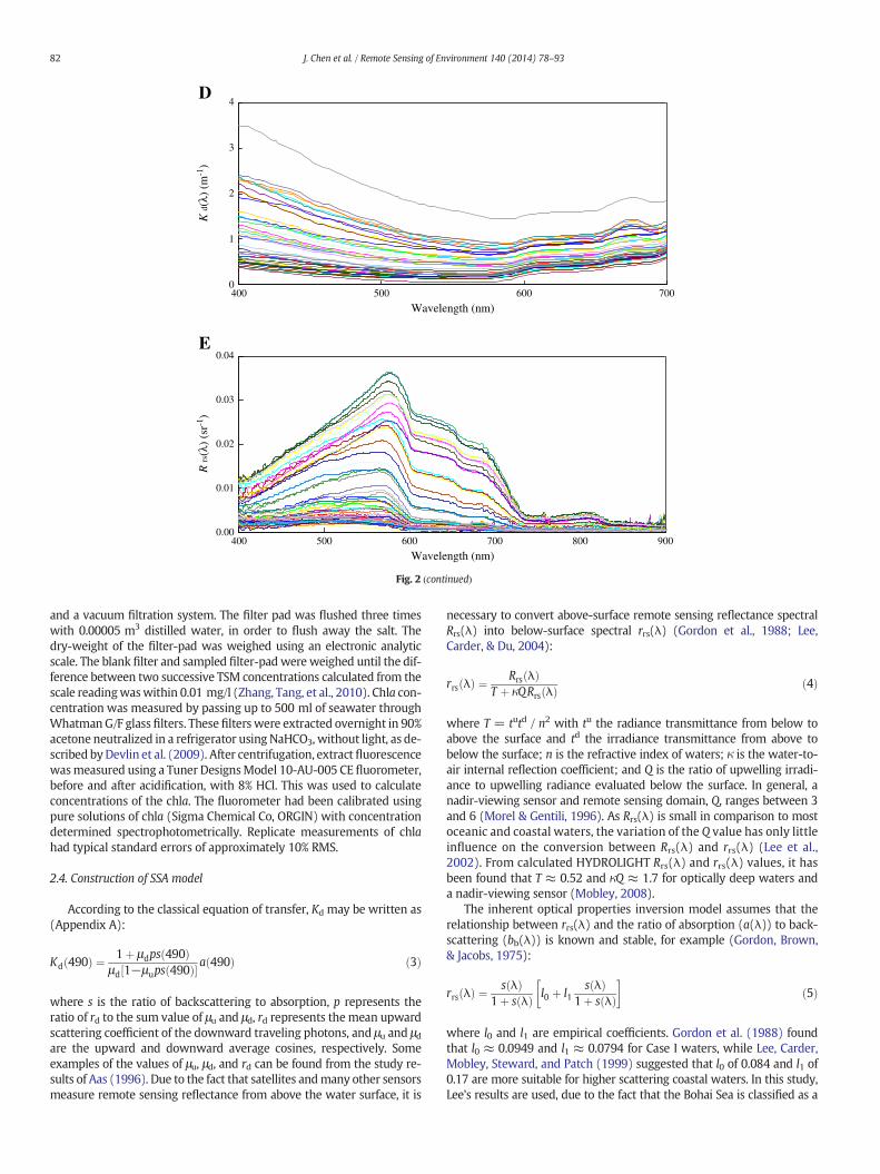
Fig. 2. Spectral curves ofRrs(λ) and kd(λ) of three independent dataset. (A) and (B) Thefirst datacollected from Bohai Sea in June 2005; and (E) the third dataset collected from Yellow Sea in 2

slope (Pierson, Kratzer, Strömbeck, & Håkansson, 2008). The measure-ments obtained in this study suggest that the first optical depth in theBohai Sea usually ranges between 0.6 and 5 m and rarely exceeds 6 m.This indicates that in this study themeasurements of underwater irradi-anceweremade to a sufficient depth, in order to accurately estimate theKd(λ). The total absorption coefficient minus pure water absorption co-efficient, denoted as at-w(λ), is measured by aWetlabs AC9 photometer.The temperature salinity and reflective tube scattering corrections wereperformed after the cruise. The correction method is described in WETLabs, Inc. (2008). The data for acdom(λ) were measured according to theSeaWiFS protocols (Mueller & Fargion, 2002).

The total suspended matter (TSM) concentration was measuredby a weighing method proposed by Mueller and Fargion (2002).Thewater samplewasfilteredwith 450 nmfilter (WhatmanGF/Ffilters)

set collected fromBohai Sea inAugust and September 2005; (C) and (D) the second dataset003.

0

1

2

3

4

400 500 600 700

Wavelength (nm)

K d

(λ)

(m-1

)

D

0.00

0.01

0.02

0.03

0.04

400 500 600 700 800 900

Wavelength (nm)

R rs

(λ)

(sr-1

)

E

Fig. 2 (continued)

82 J. Chen et al. / Remote Sensing of Environment 140 (2014) 78–93

and a vacuum filtration system. The filter pad was flushed three timeswith 0.00005 m3 distilled water, in order to flush away the salt. Thedry-weight of the filter-pad was weighed using an electronic analyticscale. The blank filter and sampled filter-pad were weighed until the dif-ference between two successive TSM concentrations calculated from thescale readingwaswithin 0.01 mg/l (Zhang, Tang, et al., 2010). Chla con-centration was measured by passing up to 500 ml of seawater throughWhatmanG/F glass filters. These filters were extracted overnight in 90%acetone neutralized in a refrigerator using NaHCO3, without light, as de-scribed byDevlin et al. (2009). After centrifugation, extract fluorescencewasmeasured using a Tuner DesignsModel 10-AU-005 CE fluorometer,before and after acidification, with 8% HCl. This was used to calculateconcentrations of the chla. The fluorometer had been calibrated usingpure solutions of chla (Sigma Chemical Co, ORGIN) with concentrationdetermined spectrophotometrically. Replicate measurements of chlahad typical standard errors of approximately 10% RMS.

2.4. Construction of SSA model

According to the classical equation of transfer, Kd may be written as(Appendix A):

Kd 490ð Þ ¼ 1þ μdps 490ð Þμd 1−μups 490ð Þ½ � a 490ð Þ ð3Þ

where s is the ratio of backscattering to absorption, p represents theratio of rd to the sum value of μu and μd, rd represents themean upwardscattering coefficient of the downward traveling photons, and μu and μdare the upward and downward average cosines, respectively. Someexamples of the values of μu, μd, and rd can be found from the study re-sults of Aas (1996). Due to the fact that satellites andmany other sensorsmeasure remote sensing reflectance from above the water surface, it is

necessary to convert above-surface remote sensing reflectance spectralRrs(λ) into below-surface spectral rrs(λ) (Gordon et al., 1988; Lee,Carder, & Du, 2004):

rrs λð Þ ¼ Rrs λð ÞT þ κQRrs λð Þ ð4Þ

where T = tutd / n2 with tu the radiance transmittance from below toabove the surface and td the irradiance transmittance from above tobelow the surface; n is the refractive index of waters; κ is the water-to-air internal reflection coefficient; and Q is the ratio of upwelling irradi-ance to upwelling radiance evaluated below the surface. In general, anadir-viewing sensor and remote sensing domain, Q, ranges between 3and 6 (Morel & Gentili, 1996). As Rrs(λ) is small in comparison to mostoceanic and coastal waters, the variation of the Q value has only littleinfluence on the conversion between Rrs(λ) and rrs(λ) (Lee et al.,2002). From calculated HYDROLIGHT Rrs(λ) and rrs(λ) values, it hasbeen found that T ≈ 0.52 and κQ ≈ 1.7 for optically deep waters anda nadir-viewing sensor (Mobley, 2008).

The inherent optical properties inversion model assumes that therelationship between rrs(λ) and the ratio of absorption (a(λ)) to back-scattering (bb(λ)) is known and stable, for example (Gordon, Brown,& Jacobs, 1975):

rrs λð Þ ¼ s λð Þ1þ s λð Þ l0 þ l1

s λð Þ1þ s λð Þ

� �ð5Þ

where l0 and l1 are empirical coefficients. Gordon et al. (1988) foundthat l0 ≈ 0.0949 and l1 ≈ 0.0794 for Case I waters, while Lee, Carder,Mobley, Steward, and Patch (1999) suggested that l0 of 0.084 and l1 of0.17 are more suitable for higher scattering coastal waters. In this study,Lee's results are used, due to the fact that the Bohai Sea is classified as a

83J. Chen et al. / Remote Sensing of Environment 140 (2014) 78–93

turbid Case IIwater. Therefore, knowing rrs(λ), s(λ)may be quickly calcu-lated using Eq. (5):

s λð Þ ¼ bb λð Þa λð Þ ¼ 2rrs λð Þ

l0 þffiffiffiffiffiffiffiffiffiffiffiffiffiffiffiffiffiffiffiffiffiffiffiffiffiffiffiffil20 þ 4l1rrs λð Þ

q−2rrs λð Þ

: ð6Þ

The backscattering coefficient may generally be expressed as afunction of the spectral irradiance reflectance just beneath the seasurface and the absorption (Gordon et al., 1988). Doron, Babin, andHembise (2007) showed that the backscattering coefficient at thewavelength 490 nm, bb(490), may be linearly related to the irradiancereflectance just beneath the surface at the wavelength 709 nm. Basedon this concept, Wang, Son, and Harding (2009) related bb(490) tothe irradiance reflectance just beneath surface at the wavelength670 nm as follows:

bb 490ð Þ ¼ C0 þ C1R 670ð Þ ð7Þ

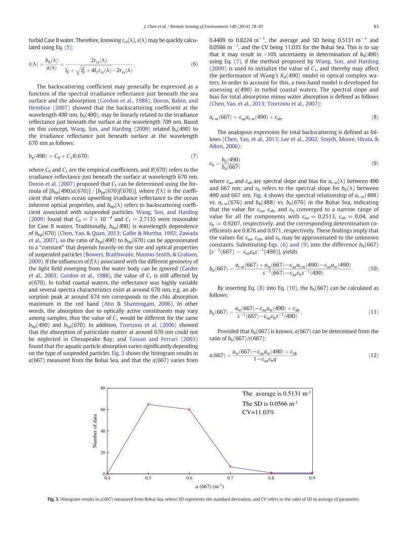
where C0 and C1 are the empirical coefficients, and R(670) refers to theirradiance reflectance just beneath the surface at wavelength 670 nm.Doron et al. (2007) proposed that C1 can be determined using the for-mula of [bbp(490)a(670)] / [bbp(670)f(670)], where f(λ) is the coeffi-cient that relates ocean upwelling irradiance reflectance to the oceaninherent optical properties, and bbp(λ) refers to backscattering coeffi-cient associated with suspended particles. Wang, Son, and Harding(2009) found that C0 = 7 × 10−4 and C1 = 2.7135 were reasonablefor Case II waters. Traditionally, bbp(490) is wavelength dependenceof bbp(670) (Chen, Yao, & Quan, 2013; Gallie & Murtha, 1992; Zawadaet al., 2007), so the ratio of bbp(490) to bbp(670) can be approximatedto a “constant” that depends heavily on the size and optical propertiesof suspended particles (Bowers, Braithwaite, Nimmo-Smith, & Graham,2009). If the influences of f(λ) associatedwith the different geometry ofthe light field emerging from the water body can be ignored (Carderet al., 2003; Gordon et al., 1988), the value of C1 is still affected bya(670). In turbid coastal waters, the reflectance was highly variableand several spectra characteristics exist at around 670 nm, e.g. an ab-sorption peak at around 674 nm corresponds to the chla absorptionmaximum in the red band (Ahn & Shanmugam, 2006). In otherwords, the absorption due to optically active constituents may varyamong samples, thus the value of C1 would be different for the samebbp(490) and bbp(670). In addition, Tzortziou et al. (2006) showedthat the absorption of particulate matter at around 670 nm could notbe neglected in Chesapeake Bay; and Tassan and Ferrari (2003)found that the aquatic particle absorption varies significantly dependingon the type of suspended particles. Fig. 3 shows the histogram results ina(667) measured from the Bohai Sea, and that the a(667) varies from

0

20

40

60

80

0.4 0.5 0.6

a (667

Num

ber

of d

ata

Fig. 3. Histogram results in a(667) measured from Bohai Sea, where SD represents th

0.4409 to 0.8224 m−1, the average and SD being 0.5131 m−1 and0.0566 m−1, and the CV being 11.03% for the Bohai Sea. This is to saythat it may result in N10% uncertainty in determination of bb(490)using Eq. (7), if the method proposed by Wang, Son, and Harding(2009) is used to initialize the value of C1, and thereby may affectthe performance of Wang's Kd(490) model in optical complex wa-ters. In order to account for this, a two-band model is developed forassessing a(490) in turbid coastal waters. The spectral slope andbias for total absorption minus water absorption is defined as follows(Chen, Yao, et al., 2013; Tzortziou et al., 2007):

at‐w 667ð Þ ¼ εaaat‐w 490ð Þ þ εab: ð8Þ

The analogous expression for total backscattering is defined as fol-lows (Chen, Yao, et al., 2013; Lee et al., 2002; Smyth, Moore, Hirata, &Aiken, 2006):

εb ¼ bb 490ð Þbb 667ð Þ ð9Þ

where εaa and εab are spectral slope and bias for at-w(λ) between 490and 667 nm; and εb refers to the spectral slope for bb(λ) between490 and 667 nm. Fig. 4 shows the spectral relationship of at-w(488)vs. at-w(676) and bb(488) vs. bb(676) in the Bohai Sea, indicatingthat the value for εaa, εab, and εb converged to a narrow range ofvalue for all the components with εaa = 0.2513, εab = 0.04, andεb = 0.9207, respectively, and the corresponding determination co-efficients are 0.876 and 0.971, respectively. These findings imply thatthe values for εaa, εab, and εb may be approximated to the unknownconstants. Substituting Eqs. (6) and (9) into the difference bb(667)[s−1(667) − εaaεbs−1(490)], yields

bb 667ð Þ ¼ at‐w 667ð Þ þ aw 667ð Þ−εaaat‐w 490ð Þ−εaaaw 490ð Þs−1 667ð Þ−εaaεbs

−1 490ð Þ : ð10Þ

By inserting Eq. (8) into Eq. (10), the bb(667) can be calculated asfollows:

bb 667ð Þ ¼ aw 667ð Þ−εaaaw 490ð Þ þ εabs−1 667ð Þ−εaaεbs

−1 490ð Þ : ð11Þ

Provided that bb(667) is known, a(667) can be determined from theratio of bb(667)/s(667):

a 667ð Þ ¼ aw 667ð Þ−εaaaw 490ð Þ þ εab1−εaaεbq

ð12Þ

0.7 0.8 0.9

) (m-1)

The average is 0.5131 m-1

The SD is 0.0566 m-1

CV=11.03%

e standard derivation, and CV refers to the ratio of SD to average of parameter.

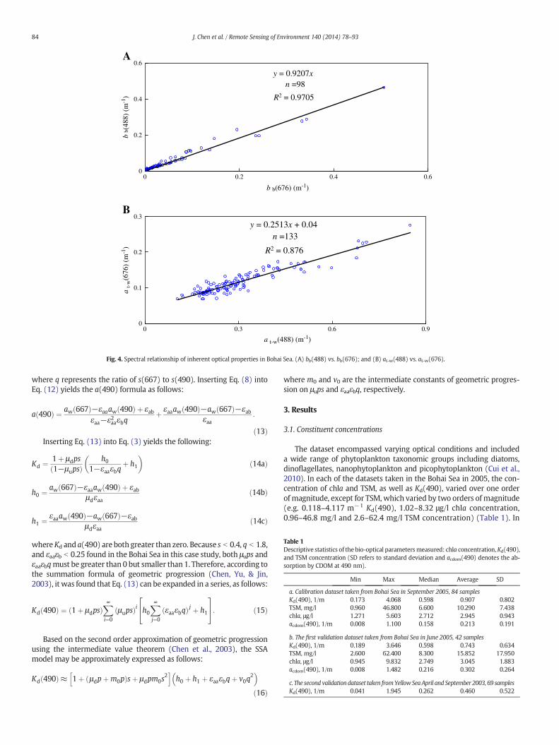
y = 0.9207x n =98

R2 = 0.9705

0

0.2

0.4

0.6

0 0.2 0.4 0.6

b b(676) (m-1)

b b(

488)

(m

-1)

A

y = 0.2513x + 0.04n =133

R2 = 0.876

0

0.1

0.2

0.3

0 0.3 0.6 0.9

a t-w(488) (m-1)

a t-

w(6

76)

(m-1

)

B

Fig. 4. Spectral relationship of inherent optical properties in Bohai Sea. (A) bb(488) vs. bb(676); and (B) at-w(488) vs. at-w(676).

Table 1Descriptive statistics of the bio-optical parametersmeasured: chla concentration,Kd(490),and TSM concentration (SD refers to standard deviation and acdom(490) denotes the ab-sorption by CDOM at 490 nm).

Min Max Median Average SD

a. Calibration dataset taken from Bohai Sea in September 2005, 84 samplesKd(490), 1/m 0.173 4.068 0.598 0.907 0.802TSM, mg/l 0.960 46.800 6.600 10.290 7.438chla, μg/l 1.271 5.603 2.712 2.945 0.943acdom(490), 1/m 0.008 1.100 0.158 0.213 0.191

b. The first validation dataset taken from Bohai Sea in June 2005, 42 samplesKd(490), 1/m 0.189 3.646 0.598 0.743 0.634TSM, mg/l 2.600 62.400 8.300 15.852 17.950chla, μg/l 0.945 9.832 2.749 3.045 1.883acdom(490), 1/m 0.008 1.482 0.216 0.302 0.264

c. The second validation dataset taken fromYellow Sea April and September 2003, 69 samplesKd(490), 1/m 0.041 1.945 0.262 0.460 0.522

84 J. Chen et al. / Remote Sensing of Environment 140 (2014) 78–93

where q represents the ratio of s(667) to s(490). Inserting Eq. (8) intoEq. (12) yields the a(490) formula as follows:

a 490ð Þ ¼ aw 667ð Þ−εaaaw 490ð Þ þ εabεaa−ε2aaεbq

þ εaaaw 490ð Þ−aw 667ð Þ−εabεaa

:

ð13ÞInserting Eq. (13) into Eq. (3) yields the following:

Kd ¼ 1þ μdps1−μupsð Þ

h01−εaaεbq

þ h1

� �ð14aÞ

h0 ¼ aw 667ð Þ−εaaaw 490ð Þ þ εabμdεaa

ð14bÞ

h1 ¼ εaaaw 490ð Þ−aw 667ð Þ−εabμdεaa

ð14cÞ

whereKd and a(490) are both greater than zero. Because s b 0.4, q b 1.8,and εaaεb b 0.25 found in the Bohai Sea in this case study, both μups andεaaεbqmust be greater than 0 but smaller than 1. Therefore, according tothe summation formula of geometric progression (Chen, Yu, & Jin,2003), it was found that Eq. (13) can be expanded in a series, as follows:

Kd 490ð Þ ¼ 1þ μdpsð ÞX∞i¼0

μupsð Þi h0X∞j¼0

εaaεbqð Þ j þ h1

24

35: ð15Þ

Based on the second order approximation of geometric progressionusing the intermediate value theorem (Chen et al., 2003), the SSAmodel may be approximately expressed as follows:

Kd 490ð Þ≈ 1þ μdpþm0pð Þsþ μdpm0s2

h ih0 þ h1 þ εaaεbqþ v0q

2�

ð16Þ

where m0 and v0 are the intermediate constants of geometric progres-sion on μups and εaaεbq, respectively.

3. Results

3.1. Constituent concentrations

The dataset encompassed varying optical conditions and includeda wide range of phytoplankton taxonomic groups including diatoms,dinoflagellates, nanophytoplankton and picophytoplankton (Cui et al.,2010). In each of the datasets taken in the Bohai Sea in 2005, the con-centration of chla and TSM, as well as Kd(490), varied over one orderof magnitude, except for TSM, which varied by two orders of magnitude(e.g. 0.118–4.117 m−1 Kd(490), 1.02–8.32 μg/l chla concentration,0.96–46.8 mg/l and 2.6–62.4 mg/l TSM concentration) (Table 1). In

85J. Chen et al. / Remote Sensing of Environment 140 (2014) 78–93

the Bohai Sea, the Kd(490), chla and TSM concentrations vary dependingon the season. In September theKd(490) varies from0.178 to 4.117 m−1,while the chla and TSM concentrations vary from1.271 to 4.718 μg/l and0.96 to 46.8 mg/l, respectively. In August the variation ranges of Kd(490)and TSM concentration were smaller, half the size of those in September(denoted in Table 1 using SD). In June the Kd(490) was smaller than thatin September but larger than that in August, while the TSM concentra-tion was larger than in these latter two months.

As in the case of the Bohai Sea in June–September 2005, Kd(490) vs.chla concentration, Kd(490) vs. TSM concentration, and Kd(490) vs.acdom(490) in these datasets (Fig. 2 and Table 1) were not significantlycorrelated, where acdom(490) refers to the absorption due to coloreddissolved organicmatter (CDOM)at 490 nm.However,whenwe ignoredoutliers with TSM N 20 mg/l, the performances of Kd(490) depended onTSM concentration increased significantly. Similarly, when we ignored

K d(490)= 0.

R 2

0

1

2

3

4

5

0 3

chla

K d

(490

) (m

-1)

A

Chla dominated water types

K d(490) = 0

R 2

0

1

2

3

4

5

0 10 20 30

TSM

K d

(490

) (m

-1)

B

TSM domina

K d(490)= 1.384an

R 2 =

0

1

2

3

4

5

0 0.4 0

a cdom(4

K d

(490

) (m

-1)

C

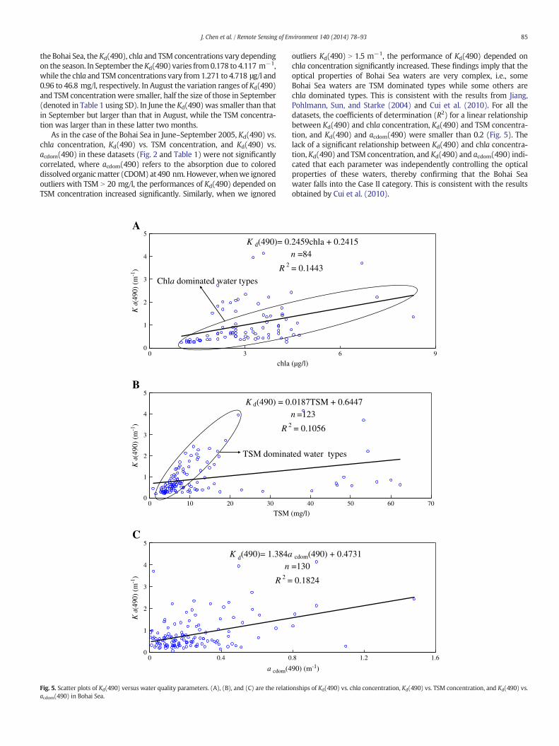
Fig. 5. Scatter plots of Kd(490) versus water quality parameters. (A), (B), and (C) are the relatioacdom(490) in Bohai Sea.

outliers Kd(490) N 1.5 m−1, the performance of Kd(490) depended onchla concentration significantly increased. These findings imply that theoptical properties of Bohai Sea waters are very complex, i.e., someBohai Sea waters are TSM dominated types while some others arechla dominated types. This is consistent with the results from Jiang,Pohlmann, Sun, and Starke (2004) and Cui et al. (2010). For all thedatasets, the coefficients of determination (R2) for a linear relationshipbetween Kd(490) and chla concentration, Kd(490) and TSM concentra-tion, and Kd(490) and acdom(490) were smaller than 0.2 (Fig. 5). Thelack of a significant relationship between Kd(490) and chla concentra-tion, Kd(490) and TSM concentration, and Kd(490) and acdom(490) indi-cated that each parameter was independently controlling the opticalproperties of these waters, thereby confirming that the Bohai Seawater falls into the Case II category. This is consistent with the resultsobtained by Cui et al. (2010).

2459chla + 0.2415n =84

= 0.1443

6 9

(µg/l)

.0187TSM + 0.6447n =123

= 0.1056

40 50 60 70

(mg/l)

ted water types

cdom(490) + 0.4731=130

0.1824

.8 1.2 1.6

90) (m-1)

nships of Kd(490) vs. chla concentration, Kd(490) vs. TSM concentration, and Kd(490) vs.

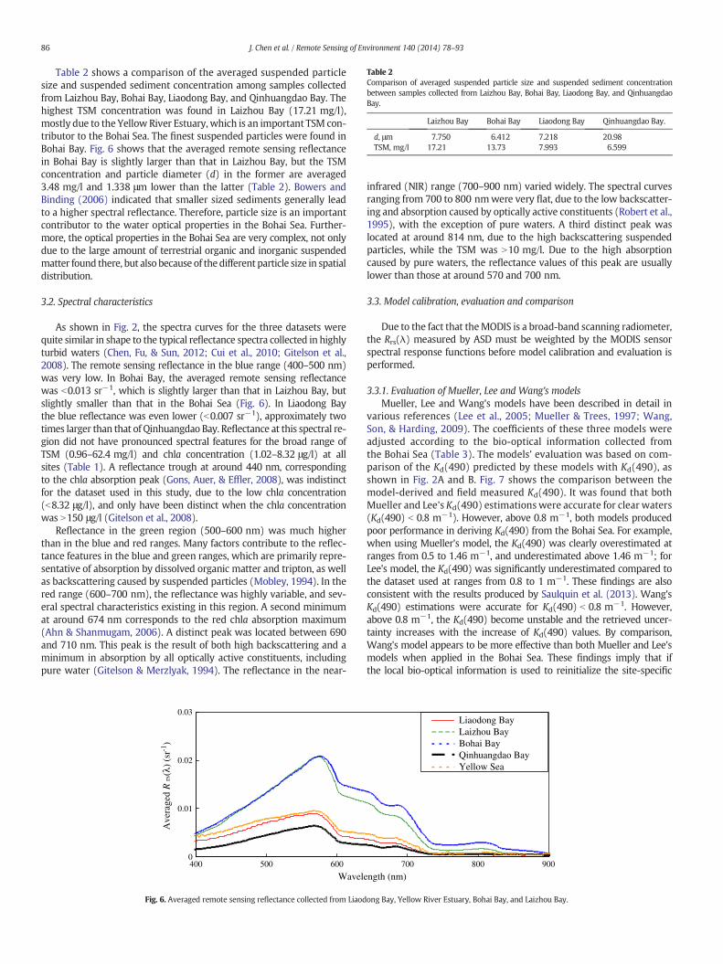
Table 2Comparison of averaged suspended particle size and suspended sediment concentrationbetween samples collected from Laizhou Bay, Bohai Bay, Liaodong Bay, and QinhuangdaoBay.

Laizhou Bay Bohai Bay Liaodong Bay Qinhuangdao Bay.

d, μm 7.750 6.412 7.218 20.98TSM, mg/l 17.21 13.73 7.993 6.599

86 J. Chen et al. / Remote Sensing of Environment 140 (2014) 78–93

Table 2 shows a comparison of the averaged suspended particlesize and suspended sediment concentration among samples collectedfrom Laizhou Bay, Bohai Bay, Liaodong Bay, and Qinhuangdao Bay. Thehighest TSM concentration was found in Laizhou Bay (17.21 mg/l),mostly due to the Yellow River Estuary, which is an important TSM con-tributor to the Bohai Sea. The finest suspended particles were found inBohai Bay. Fig. 6 shows that the averaged remote sensing reflectancein Bohai Bay is slightly larger than that in Laizhou Bay, but the TSMconcentration and particle diameter (d) in the former are averaged3.48 mg/l and 1.338 μm lower than the latter (Table 2). Bowers andBinding (2006) indicated that smaller sized sediments generally leadto a higher spectral reflectance. Therefore, particle size is an importantcontributor to the water optical properties in the Bohai Sea. Further-more, the optical properties in the Bohai Sea are very complex, not onlydue to the large amount of terrestrial organic and inorganic suspendedmatter found there, but also because of thedifferent particle size in spatialdistribution.

3.2. Spectral characteristics

As shown in Fig. 2, the spectra curves for the three datasets werequite similar in shape to the typical reflectance spectra collected in highlyturbid waters (Chen, Fu, & Sun, 2012; Cui et al., 2010; Gitelson et al.,2008). The remote sensing reflectance in the blue range (400–500 nm)was very low. In Bohai Bay, the averaged remote sensing reflectancewas b0.013 sr−1, which is slightly larger than that in Laizhou Bay, butslightly smaller than that in the Bohai Sea (Fig. 6). In Liaodong Baythe blue reflectance was even lower (b0.007 sr−1), approximately twotimes larger than that of Qinhuangdao Bay. Reflectance at this spectral re-gion did not have pronounced spectral features for the broad range ofTSM (0.96–62.4 mg/l) and chla concentration (1.02–8.32 μg/l) at allsites (Table 1). A reflectance trough at around 440 nm, correspondingto the chla absorption peak (Gons, Auer, & Effler, 2008), was indistinctfor the dataset used in this study, due to the low chla concentration(b8.32 μg/l), and only have been distinct when the chla concentrationwas N150 μg/l (Gitelson et al., 2008).

Reflectance in the green region (500–600 nm) was much higherthan in the blue and red ranges. Many factors contribute to the reflec-tance features in the blue and green ranges, which are primarily repre-sentative of absorption by dissolved organic matter and tripton, as wellas backscattering caused by suspended particles (Mobley, 1994). In thered range (600–700 nm), the reflectance was highly variable, and sev-eral spectral characteristics existing in this region. A second minimumat around 674 nm corresponds to the red chla absorption maximum(Ahn & Shanmugam, 2006). A distinct peak was located between 690and 710 nm. This peak is the result of both high backscattering and aminimum in absorption by all optically active constituents, includingpure water (Gitelson & Merzlyak, 1994). The reflectance in the near-

0

0.01

0.02

0.03

400 500 600

Wavel

Ave

rage

d R

rs(λ

) (s

r-1)

Fig. 6. Averaged remote sensing reflectance collected from Liaod

infrared (NIR) range (700–900 nm) varied widely. The spectral curvesranging from 700 to 800 nmwere very flat, due to the low backscatter-ing and absorption caused by optically active constituents (Robert et al.,1995), with the exception of pure waters. A third distinct peak waslocated at around 814 nm, due to the high backscattering suspendedparticles, while the TSM was N10 mg/l. Due to the high absorptioncaused by pure waters, the reflectance values of this peak are usuallylower than those at around 570 and 700 nm.

3.3. Model calibration, evaluation and comparison

Due to the fact that theMODIS is a broad-band scanning radiometer,the Rrs(λ) measured by ASD must be weighted by the MODIS sensorspectral response functions before model calibration and evaluation isperformed.

3.3.1. Evaluation of Mueller, Lee and Wang's modelsMueller, Lee and Wang's models have been described in detail in

various references (Lee et al., 2005; Mueller & Trees, 1997; Wang,Son, & Harding, 2009). The coefficients of these three models wereadjusted according to the bio-optical information collected fromthe Bohai Sea (Table 3). The models' evaluation was based on com-parison of the Kd(490) predicted by these models with Kd(490), asshown in Fig. 2A and B. Fig. 7 shows the comparison between themodel-derived and field measured Kd(490). It was found that bothMueller and Lee's Kd(490) estimations were accurate for clear waters(Kd(490) b 0.8 m−1). However, above 0.8 m−1, both models producedpoor performance in deriving Kd(490) from the Bohai Sea. For example,when using Mueller's model, the Kd(490) was clearly overestimated atranges from 0.5 to 1.46 m−1, and underestimated above 1.46 m−1; forLee's model, the Kd(490) was significantly underestimated compared tothe dataset used at ranges from 0.8 to 1 m−1. These findings are alsoconsistent with the results produced by Saulquin et al. (2013). Wang'sKd(490) estimations were accurate for Kd(490) b 0.8 m−1. However,above 0.8 m−1, the Kd(490) become unstable and the retrieved uncer-tainty increases with the increase of Kd(490) values. By comparison,Wang's model appears to be more effective than both Mueller and Lee'smodels when applied in the Bohai Sea. These findings imply that ifthe local bio-optical information is used to reinitialize the site-specific

700 800 900

ength (nm)

Liaodong BayLaizhou BayBohai BayQinhuangdao BayYellow Sea

ong Bay, Yellow River Estuary, Bohai Bay, and Laizhou Bay.

Table 3Kd(490) quantitative retrieval models.

Model Adjusted model R2

Mueller1:446−2:289

Rrs 490ð ÞRrs 555ð Þ

� �4:252 0.1367

Lee (1 + 0.005θs)a(490) + 25.981[1.0 − 0.52e−1.8a(490)]bb(490) 0.5087Wang 2:13� 10−4

Rrs 488ð Þ þ 0:8245Rrs 667ð ÞRrs 488ð Þ þ 3:657 18:877Rrs 667ð Þ−0:0165½ � 1−0:52e−

2:533�10−3Rrs 488ð Þ −9:817

Rrs 667ð ÞRrs 488ð Þ

" #0.8841

87J. Chen et al. / Remote Sensing of Environment 140 (2014) 78–93

coefficients of Wang's model, then Wang's model produces a good per-formance in deriving Kd(490) from the Bohai Sea, which has a coefficientof determination (R2) of 0.8841.

3.3.2. SSA model calibrationThe band tuning technique was used to determine the optimal posi-

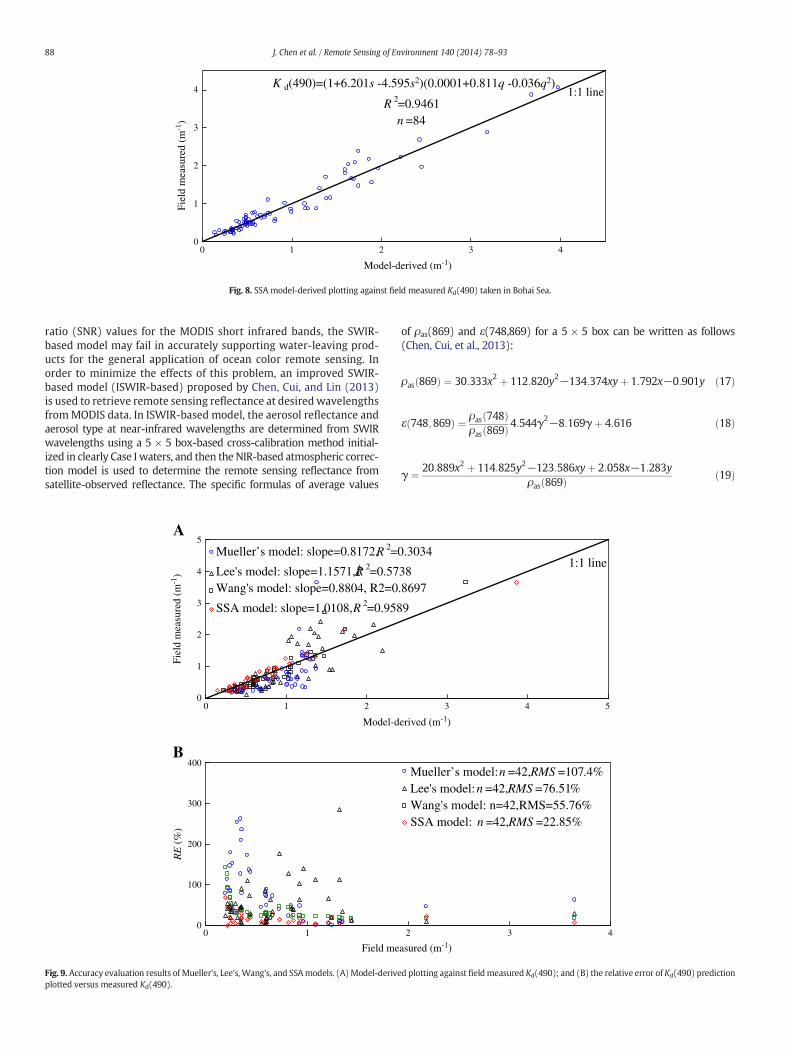
tions forλi and λj in the SSAmodel, i.e. in order to determine the optimalpositions and constant coefficients of the SSA model, λi and λj were de-termined by bands tuning from 412 to 869 nm using MODIS spectralbands. The recursive procedures proposed by Chen and Quan (2013)were used to identify the best fit function of Eq. (16). RMS values, asshown in Eq. (2), were used to determine the optimal bands and con-stant coefficients of the SSA model. The optimal SSA model must havethe minimum RMS value. For the purpose of prediction, statistical re-gression relationships were established between the SSA model and insitu Kd(490) taken in September 2005 (Fig. 2A and B). Based on 84field samples, the semi-analytical model shown in Fig. 8 was proposedas the optimal SSA model in quantifying Kd(490) from the Bohai Sea. Itwas found that the optimal bands of the SSA model were λi = 490 nmand λj = 667 nm, and that the corresponding correlation coefficient be-tween the retrieved Kd(490) and in situ measurements was 0.941. Theresults indicate that the SSA model is an effective predictor in derivingKd(490) with MODIS spectral bands in the turbid coastal waters of theBohai Sea.

3.3.3. Model evaluation and comparisonIn this section of the paper, an evaluation ofMueller, Lee andWang's

models and the SSAmodel withMODIS spectral bands is presented. Theevaluation was based on the comparison of the Kd(490) predicted bythese algorithms, with Kd(490) measured analytically for the indepen-dent dataset collected from the Bohai Sea in June 2005 (Fig. 2C and D).Comparisons of the measured and predicted estimates of Kd(490) byMueller, Lee and Wang's models and the SSA model with MODIS spec-tral bands are presented in Fig. 9A. It was found that the SSA model(RMS = 22.85%) had a superior performance in comparison to Mueller(RMS = 107.4%), Lee (RMS = 76.51%) and Wang's (RMS = 55.76%)models. Using the SSA model for retrieving Kd(490) in the Bohai Sea

1

2

3

4

0 1 2

Model-de

Fiel

d m

easu

red

(m-1

)

Mueller’s modelLee's modelWang's model

0

Fig. 7.Mueller's, Lee's, and Wang's models-derived plo

decreased by 84.55% RMS from Mueller's model, 53.66% RMS fromLee's model, and 32.91% RMS from Wang's model. It appears that onlythe SSA model and Wang's model may be used to retrieve Kd(490)from turbid Case II waters, but in thesewaters the SSAmodel ismore ef-fective thanWang's model.

The relationship between RE and Kd(490) was also presented todemonstrate the ability of these four models in estimating Kd(490)(Fig. 9B). It was found that the RE value decreases with increasingKd(490) values, but there is no statistically significant relationship be-tween the two. For the range of Kd(490) from 0.18 to 3.65 m−1, theRE of Kd(490) predicted by the SSAmodel was below 50%, with an aver-age of 22.85% of the observed Kd(490). The slopes of the linear relation-ships between SSA model-derived and in situ measured Kd(490) was1.01. Comparison of the SSA model to that of other three models indi-cates that the SSAmodel considerably reduces the RE value and outper-formsMueller, Lee andWang'smodels, especially at a low Kd(490) level(b0.5 m−1). These findings imply that the SSA model does not requirefurther optimization of spectral band positions and site-specific pa-rameterization to accurately estimate Kd(490) in water bodies withwidely varying bio-optical characteristics taken in different seasonsin the Bohai Sea.

3.4. Kd(490) retrieval in the Bohai Sea

Due to the poor performance of Mueller and Lee's models in theBohai Sea, only Wang's model and the SSA model are discussed in thissection of the paper.

3.4.1. Atmospheric correctionDue to the fact that the majority of the Bohai Sea water falls into the

Case II category (Cui et al., 2010), classical methods of atmospheric cor-rection (NIR-based model) (Gordon & Wang, 1994; Gould & Arnone,1997) may be violated in these waters. Wang, Son, and Shi (2009),Wang, Tang, and Shi (2007) proposed an atmospheric correction algo-rithm which uses the shortwave infrared bands (SWIR-based model)to improve ocean color products in turbid coastal waters measured bythe MODIS. However, due to the considerably lower sensor signal–noise

1:1 line

3 4

rived (m-1)

tting against field measured Kd(490), 84 samples.

1:1 line

1

2

3

4

0 1 2 3 4

Model-derived (m-1)

Fiel

d m

easu

red

(m-1

)

K d(490)=(1+6.201s -4.595s2)(0.0001+0.811q -0.036q2)

R 2=0.9461n =84

0

Fig. 8. SSA model-derived plotting against field measured Kd(490) taken in Bohai Sea.

88 J. Chen et al. / Remote Sensing of Environment 140 (2014) 78–93

ratio (SNR) values for the MODIS short infrared bands, the SWIR-based model may fail in accurately supporting water-leaving prod-ucts for the general application of ocean color remote sensing. Inorder to minimize the effects of this problem, an improved SWIR-based model (ISWIR-based) proposed by Chen, Cui, and Lin (2013)is used to retrieve remote sensing reflectance at desired wavelengthsfromMODIS data. In ISWIR-based model, the aerosol reflectance andaerosol type at near-infrared wavelengths are determined from SWIRwavelengths using a 5 × 5 box-based cross-calibration method initial-ized in clearly Case I waters, and then the NIR-based atmospheric correc-tion model is used to determine the remote sensing reflectance fromsatellite-observed reflectance. The specific formulas of average values

1

2

3

4

5

0 1 2

Model-d

Fiel

d m

easu

red

(m-1

)

Mueller’s model: slope=0.8172, R 2=0

Lee's model: slope=1.1571, R 2=0.57Wang's model: slope=0.8804, R2=0

SSA model: slope=1.0108, R 2=0.958

A

0

100

200

300

400

0 1

Field me

RE

(%

)

B

0

Fig. 9.Accuracy evaluation results of Mueller's, Lee's, Wang's, and SSAmodels. (A)Model-deriveplotted versus measured Kd(490).

of ρas(869) and ε(748,869) for a 5 × 5 box can be written as follows(Chen, Cui, et al., 2013):

ρas 869ð Þ ¼ 30:333x2 þ 112:820y2−134:374xyþ 1:792x−0:901y ð17Þ

ε 748;869ð Þ ¼ ρas 748ð Þρas 869ð Þ4:544γ

2−8:169γ þ 4:616 ð18Þ

γ ¼ 20:889x2 þ 114:825y2−123:586xyþ 2:058x−1:283yρas 869ð Þ ð19Þ

1:1 line

3 4 5

erived (m-1)

.3034

38.8697

9

2 3 4

asured (m-1)

Mueller’s model:n =42,RMS =107.4%Lee's model:n =42,RMS =76.51%Wang's model: n=42,RMS=55.76%SSA model: n =42,RMS =22.85%

d plotting against fieldmeasured Kd(490); and (B) the relative error of Kd(490) prediction

1:1 line

0.01

0.02

0.03

0 0.01 0.02 0.03

Model-derived (sr-1)

Fiel

d m

easu

red

(sr-1

)

R rs(488),n =31,RMS =17.41%

R rs(667),n =26,RMS =18.93%

0

Fig. 10. ISWIR-based model-derived plotted against field measured remote sensing reflectance.

89J. Chen et al. / Remote Sensing of Environment 140 (2014) 78–93

where x and y refer to ρas(1240) and ρas(2130), respectively, and ρasrefers to the aerosol scattering reflectance.

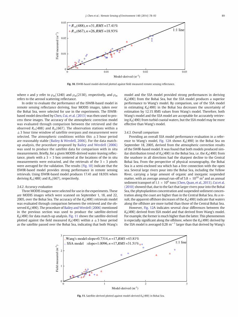
In order to evaluate the performance of the ISWIR-based model inremote sensing reflectance deriving, four MODIS images, taken overthe Bohai Sea, were selected for use in the experiments. The ISWIR-basedmodel described by Chen, Cui, et al. (2013)was then used to pro-cess these images. The accuracy of the atmospheric correction modelwas evaluated through comparison between the retrieved and theobserved Rrs(488) and Rrs(667). The observation stations within a±3 hour time window of satellite overpass and measurement wereselected. The atmospheric conditions within this ±3 hour periodare reasonably stable (Bailey & Werdell, 2006). For the data match-up analysis, the procedure proposed by Bailey and Werdell (2006)was used to produce the satellite data for comparison with in situmeasurements. Briefly, for a givenMODIS-derived water-leaving reflec-tance, pixels with a 3 × 3 box centered at the locations of the in situmeasurements were extracted, and the retrievals of the 3 × 3 pixelswere averaged for the validation. The results (Fig. 10) indicate that theISWIR-based model provides strong performance in remote sensingretrievals. Using ISWIR-based model produces 17.41 and 18.93% whenderiving Rrs(488) and Rrs(667), respectively.

3.4.2. Accuracy evaluationThreeMODIS imageswere selected for use in the experiments. These

are MODIS images which were scanned on September 1, 18, and 22,2005, over the Bohai Sea. The accuracy of the Kd(490) retrievals modelwas evaluated through comparison between the retrieved and the ob-served Kd(490). The procedure of Bailey andWerdell (2006)mentionedin the previous section was used to produce the satellite-derivedKd(490) for data match-up analysis. Fig. 11 shows the satellite-derivedplotted against the field measured Kd(490) within a ±3 hour periodas the satellite passed over the Bohai Sea, indicating that both Wang's

1

2

3

0 1

Model-de

Fiel

d m

easu

red

(m-1

)

Wang's model:slope=0.7314,n =17,RMSSSA model :slope=1.0096, n =17,RMS

0

Fig. 11. Satellite-derived plotted against m

model and the SSA model provided strong performances in derivingKd(490) from the Bohai Sea, but the SSA model produces a superiorperformance to Wang's model. By comparison, use of the SSA modelin estimating Kd(490) in the Bohai Sea decreases the uncertainty ofestimation by 12.1% RMS values from Wang's model. Therefore, bothWang's model and the SSA model are acceptable for accurately retriev-ing Kd(490) from turbid coastal waters, but the SSAmodelmay bemoreeffective than Wang's model.

3.4.3. Overall comparisonProviding an overall SSA model performance evaluation in a refer-

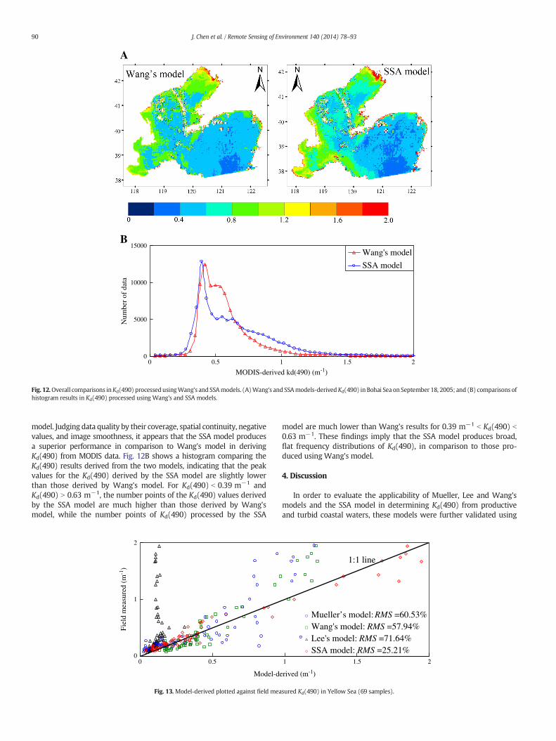
ence to Wang's model, Fig. 12A shows Kd(490) in the Bohai Sea onSeptember 18, 2005, derived from the atmospheric correction resultsof the SWIR-basedmodel. It was found that bothmodels produced sim-ilar distribution trend of Kd(490) in the Bohai Sea, i.e. the Kd(490) fromthe seashore in all directions had the sharpest decline to the CentralBohai Sea. From the perspective of physical oceanography, the BohaiSea is a semi-enclosed sea which has a free connection with the opensea. Several large rivers pour into the Bohai Sea, including the YellowRiver, carrying a large amount of organic and inorganic suspendedmatter, with an average annual run-off of 5.8 × 1010 m3 and an annualsediment transport of 1.1 × 109 tons (Chen, Quan, et al., 2013). Cui et al.(2010) showed that, due to the fact that larger rivers pour into the BohaiSea, the phytoplankton concentration and suspended sediment concen-tration along the coast are higher than in the Central Bohai Sea. As a re-sult, the apparent offshore decreases of the Kd(490) indicate thatwatersalong the offshore are more turbid than those of the Central Bohai Sea.

However, Fig. 12A indicates several clear differences between theKd(490) derived from SSA model and that derived from Wang's model.For example, the former ismuchhigher than the latter. This phenomenonis especially significant along the offshore, where the Kd(490) derived bythe SSA model is averaged 0.28 m−1 larger than that derived by Wang's

1:1 line

2 3

rived (m-1)

=43.81%=31.51%

odel-derived Kd(490) in Bohai Sea.

0

5000

10000

15000

0 0.5 1 1.5 2

MODIS-derived kd(490) (m-1)

Num

ber

of d

ata

Wang's model

SSA model

A

B

Fig. 12.Overall comparisons inKd(490) processedusingWang's and SSAmodels. (A)Wang's and SSAmodels-derivedKd(490) in Bohai Sea on September 18, 2005; and (B) comparisons ofhistogram results in Kd(490) processed using Wang's and SSA models.

90 J. Chen et al. / Remote Sensing of Environment 140 (2014) 78–93

model. Judging data quality by their coverage, spatial continuity, negativevalues, and image smoothness, it appears that the SSA model producesa superior performance in comparison to Wang's model in derivingKd(490) from MODIS data. Fig. 12B shows a histogram comparing theKd(490) results derived from the two models, indicating that the peakvalues for the Kd(490) derived by the SSA model are slightly lowerthan those derived by Wang's model. For Kd(490) b 0.39 m−1 andKd(490) N 0.63 m−1, the number points of the Kd(490) values derivedby the SSA model are much higher than those derived by Wang'smodel, while the number points of Kd(490) processed by the SSA

1

2

0 0.5

Model-d

Fiel

d m

easu

red

(m-1

)

0

Fig. 13. Model-derived plotted against field mea

model are much lower than Wang's results for 0.39 m−1 b Kd(490) b

0.63 m−1. These findings imply that the SSA model produces broad,flat frequency distributions of Kd(490), in comparison to those pro-duced using Wang's model.

4. Discussion

In order to evaluate the applicability of Mueller, Lee and Wang'smodels and the SSA model in determining Kd(490) from productiveand turbid coastal waters, these models were further validated using

1:1 line

1 1.5 2

erived (m-1)

Mueller’s model: RMS =60.53%Wang's model: RMS =57.94%Lee's model: RMS =71.64%SSA model: RMS =25.21%

sured Kd(490) in Yellow Sea (69 samples).

91J. Chen et al. / Remote Sensing of Environment 140 (2014) 78–93

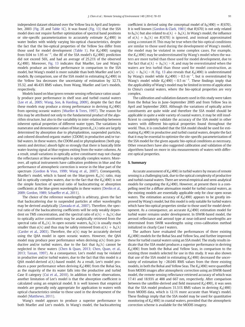
independent dataset obtained over the Yellow Sea in April and Septem-ber, 2003 (Fig. 2E and Table 1C). It was found (Fig. 13) that the SSAmodel does not require further optimization of spectral band positionsor site-specific parameterization to accurately estimate Kd(490) inwater bodies with widely varying bio-optical characteristics, despitethe fact that the bio-optical properties of the Yellow Sea differ fromthose used for model development (Table 1). For Kd(490) rangingfrom 0.04 to 1.95 m−1, the RE of the SSA model's Kd(490) predictiondid not exceed 56%, and had an average of 25.21% of the observedKd(490). Moreover, Fig. 13 indicates that Mueller, Lee and Wang'smodels produce an inferior performance in comparison to the SSAmodel, but Wang's model is more suitable than both Mueller and Lee'smodels. By comparison, use of the SSA model in estimating Kd(490) inthe Yellow Sea decreases the uncertainty of estimation by 32.73,35.32, and 46.43% RMS values, from Wang, Mueller and Lee's models,respectively.

Models based on blue/green remote sensing reflectance ratios usual-ly produce poor performance in shelf seas and turbid coastal waters(Lee et al., 2005; Wang, Son, & Harding, 2009), despite the fact thatthese models may produce a strong performance in deriving Kd(490)from opening oceanic waters (Mueller & Trees, 1997). The reason forthis may be attributed not only to the fundamental product of the algo-rithm structure, but also to the variability in inter-relationship betweeninherent optical properties of different water types. The variations innumerator and denominator values of blue/green Rrs(λ) ratio are largelydetermined by absorption due to phytoplankton, suspended particles,and colored dissolved organic matter (CDOM) in productive and/or tur-bid waters. In these waters, the CDOMand/or phytoplankton (both pig-ments and detritus) absorb light so strongly that there is basically littlewater-leaving signal at blue regions exiting from the water columns. Asa result, small variations in optically active constituent may not changethe reflectance at blue wavelengths in optically complex waters. More-over, all optical instruments have calibration problems in blue and theperformance of atmospheric correction is worse in the blue part of thespectrum (Gordon & Voss, 1999; Wang et al., 2007). Consequently,Mueller's model, which is based on the blue/green Rrs(λ) ratio, mayfail in optically complex waters, due to the fact that the Kd(490) is notthe simple function of spectral ratio of backscattering or absorptioncoefficients at the blue-green wavelengths in these waters (Devlin et al.,2009; Gordon, 1989; Schaeffer et al., 2011).

The choice of the reference wavelength is arbitrary, given the factthat backscattering due to suspended particles at other wavelengthsmay be derived analytically (Zawada et al., 2007). Therefore, the spec-tral ratio of the backscattering coefficients will be only weakly depen-dent on TMS concentration, and the spectral ratio of a(λ) + bb(λ) dueto optically active constituents may be analytically retrieved from thespectral ratio of Rrs(λ). In open oceanic waters, bb(λ) is usually muchsmaller than a(λ) and thus may be safely removed from a(λ) + bb(λ)(Carder et al., 2003). Therefore, the a(λ) may be accurately derivedusing the QAA model in open oceanic waters. However, the QAAmodel may produce poor performance when deriving a(λ) from pro-ductive and/or turbid waters, due to the fact that bb(λ) cannot beneglected in these waters (Chen & Quan, 2013; Chen, Quan, et al.,2013; Tassan, 1997). As a consequence, Lee's model may be violatedin productive and/or turbid waters, due to the fact that this model is aQAA model-derived a(λ)-based model. As a result, Lee's model pro-duces a poor performance when deriving Kd(490) from the Bohai Sea,as the majority of the its water falls into the productive and turbidCase II category (Cui et al., 2010). In addition to these observations,another limitation of Lee's model is that the absorption coefficient iscalculated using an empirical model. It is well known that empiricalmodels are generally only appropriate for application to waters withoptical characteristics similar to those used in the development of themodel (Matthews, 2011).

Wang's model appears to produce a superior performance toboth Mueller and Lee's models. In Wang's model, the backscattering

coefficient is derived using the conceptual model of bb(490) ∝ R(670).It is well known (Gordon & Clark, 1981) that R(670) is not only relatedto bb(λ) but also related to a(λ) + bb(λ). InWang's model, the influenceof a(λ) + bb(λ) on R(670) is ignored, and instead approximatedusing a constant H. This may be true when the bio-optical conditionsare similar to those used during the development of Wang's model,the model may be violated in some complex cases. For example,the Kd(490) may be underestimated by Wang's model when the wa-ters are more turbid than those used for model development, due tothe fact that a(λ) + bb(λ) N H, and may be overestimated when thewaters are less turbid than those used for model construction, asa(λ) + bb(λ) b H. Fig. 13 also reveals that Kd(490) is underestimatedby Wang's model while Kd(490) N 0.5 m−1, but is overestimated byWang's model while Kd(490) b 0.5 m−1. These findings imply thatthe applicability ofWang'smodelmay be limited in terms of applicationto China's coastal waters, where the bio-optical properties are verycomplex.

The calibration and validation datasets used in this studywere takenfrom the Bohai Sea in June–September 2005 and from Yellow Sea inApril and September 2003. Although the variations of optically activeconstituents are quite wide and therefore the SSA model should beapplicable in quite a wide variety of coastal waters, it may be still insuf-ficient to completely validate the accuracy of the SSA model in otherwaters with different bio-optical properties found throughout theworld. Thus, it is concluded that the SSA model should be used for esti-mating Kd(490) in productive and turbid coastal waters, despite the factthat it may be essential to optimize the site-specific parameterization ofthe SSAmodel for the given aquatic bio-optical conditions as necessary.Other researchers have also suggested calibration and validation of thealgorithms based on more in situ measurements of waters with differ-ent optical properties.

5. Summary

Accurate assessment ofKd(490) in turbidwaters bymeans of remotesensing is a challenging task, due to the optical complexity of productiveand turbid coastalwaters. There are several empirical and semi-analyticalmodels for computing the Kd(490). However, at present there is a com-pelling need for a diffuse attenuation model for turbid coastal waters, asthe existing models are essentially applicable only for clear open oceanwaters. The estimation accuracy of Kd(490) appears to be greatly im-proved byWang'smodel, but thismodel is only suitable for turbidwaterswhich have bio-optical properties similar to those used for model devel-opment. As a consequence, an accurate Kd(490) estimation model forturbid water remains under development. In ISWIR-based model, theaerosol reflectance and aerosol type at near-infrared wavelengths aredetermined from SWIR wavelengths using cross-calibration methodinitialized in clearly Case I waters.

The authors have evaluated the performances of three existingKd(490)models for the Bohai Sea and Yellow Sea, and further improvedthese for turbid coastal waters using an SSAmodel. The study results in-dicate that the SSA model produces a superior performance in derivingKd(490) from both the Bohai and Yellow Seas, in comparison to theexisting three models selected for use in this study. It was also shownthat use of the SSA model in estimating Kd(490) decreased the uncer-tainty of estimation by N28.04% RMS values from the three existingmodels, in both the Bohai and Yellow Seas. The Kd(490)were quantifiedfromMODIS images after atmospheric correction using an ISWIR-basedmodel, the remote sensing reflectance retrieved accuracy of which was17.41 and 18.93% at 488 and 667 nm, respectively. After comparisonbetween the satellite-derived and field measured Kd(490), it was seenthat the SSA model produces 31.51% RMS values in deriving Kd(490)from MODIS data, which is 12.1% more accurate than Wang's model.These findings imply that the SSA model may be used for quantitativemonitoring of Kd(490) in coastal waters, provided that the atmosphericcorrection scheme is available for the MODIS imagery.

92 J. Chen et al. / Remote Sensing of Environment 140 (2014) 78–93

Acknowledgments

This study is supported by the China State Major Basic ResearchProject (2013CB429701), Projects of International Cooperation and Ex-changes of National Natural Science Foundation of China (41210005),Science Foundation for 100 Excellent Youth Geological Scholars of ChinaGeological Survey, Serial Maps of Geology and Geophysics on China Seasand Landon the Scale of 1:1000000 (200311000001), High-techResearchand Development Program of China (No. 2007AA092102), Dragon 3Project (ID 10470), the Fundamental Research Funds for the CentralUniversities (No. 11CX05015A), and National Natural Science Foun-dation of China (No. 61371189). We would just like to express ourgratitude to two anonymous reviewers for their useful commentsand suggestions.

Appendix A

The radiative transfer equation for radiance L(z,μ) in seawater whichis stratified in plane layers may be written as follows (McCormick &Francisco, 1995):

μ∂L∂zþ cL ¼ b

Z 1

−1β μ; μ ′�

Ldμ ′ ðA1Þ

where z is the depthmeasured beneath the surface; μ is the cosine of thepolar angle definedwith respect to the downward direction; c = a + bis the sum of the absorption and scattering coefficients; β(μ, μ′) is thescattering function for light scattered with direction μ from directionμ′; and λ is the wavelength.

After integrating the radiative transfer equation for all directions ofthe light field, is the following formula is obtained (Kylling & Stamnes,1995):

ddz

Ed−Euð Þ ¼ −a E0d þ E0uð Þ: ðA2Þ

When the integration of Eq. (A1) is limited to the downward hemi-sphere, the result becomes the following:

dEddz

¼ aμd

þ rdbbμd

� �Ed þ

rubbμu

Eu ðA3Þ

where the index d denotes downward and u upward; Ed and Eu are thedownward and upward irradiances; E0d and E0u are the scalar mean thedownward; μd and μu are the downward and upward average cosines,respectively; and rd refers to the mean upward scattering coefficientof the downward traveling photons, while ru refers to the meandownward scattering coefficient of the upward traveling photons,with both coefficients normalized with the backward scattering co-efficient. The advantage of two-stream models compared to singlescattering models is that they contain the effects of multiple scatter-ing. Their disadvantage is that, in this study, they cannot predict thechange in the shape of the radiance distribution with depth, due tothe fact that the main focus of this study is Kd retrievals. Provided thatthe waters are sufficiently deep that reflected light from the bottomdoes not influence the irradiance of the upper layer, all irradiance mea-surements show that a first approximation of Ed should be of the follow-ing form (Gordon, 1989):

Ed zð Þ ¼ Ed 0ð Þ exp Kdzð Þ: ðA4Þ

The irradiance ratio ρ is defined as the ratio between upward anddownward irradiance (Morel & Gentili, 1996):

ρ ¼ Eu zð ÞEd zð Þ : ðA5Þ

Substituting Eq. (A4) into Eq. (A2) yields a useful relation between ρand Kd (Mobley, 1994):

Kd ¼ μu þ μdρμuμd 1−ρð Þ a: ðA6Þ

By inserting Eq. (A4) in Eq. (A3), the following may be observed(Aas, 1996):

ρ≈ μurdμu þ μd

s ðA7Þ

where s is the ratio of backscattering to absorption. When insertingEq. (A6) into Eq. (A7), the result becomes the following:

Kd ¼ 1þ μdpsμd 1−μupsð Þ a ðA8Þ

where p represents the ratio of rd to the sum value of μu and μd.

References

Aas, E. (1996). Two-stream irradiancemodel for deepwaters. Applied Optics, 11, 2095–2102.Ahn, Y. -H., & Shanmugam, P. (2006). Detecting the red tide algal blooms from satellite ocean

color observations in optically complexNortheast-Asia Coastalwaters.Remote Sensing ofEnvironment, 103, 419–437.

Austin, R. W., & Petzold, T. (1981). The determination of the diffuse attenuation coefficient ofsea water using the Coastal Zone Colour Scanner. New York: Springer, 239–256.

Bailey, S. W., & Werdell, P. J. (2006). A multi-sensor approach for the on-orbit validationof ocean color satellite data products. Remote Sensing of Environment, 102, 12–23.

Barale, V. (1987). Remote observations of the marine environment: Spatial heterogeneityof the mesoscale ocean color field in CZCS imagery of California near-coastal waters.Remote Sensing of Environment, 22, 173–186.

Bowers, D.G., & Binding, C. E. (2006). The optical properties of mineral suspended parti-cles: A review and synthesis. Estuarine, Coastal and Shelf Science, 67, 219–230.

Bowers, D.G., Braithwaite, K. M., Nimmo-Smith, W. A.M., & Graham, G. W. (2009). Lightscattering by particles suspended in the sea: The role of particle size and density.Continental Shelf Research, 29, 1748–1755.

Bukata, R. P., Jerome, J. H., Kondratyev, K. Y., & Pozdnyakov, D.V. (1995). Optical propertiesand remote sensing of inland and coastal waters (1st ed.)New York: CRC Press.

Carder, K. L., Chen, F. R., Lee, Z. P., Hawes, S. K., & Cannizzaro, J. P. (2003).MODIS OceanScience Team algorithm theoretical basis document: Case 2 chlorophyll a. (ATBD 19,Version 7).

Carter, C. M., Ross, A. H., Schiel, D. R., Howard-Williams, C., & Hayden, B. (2005). In situmicrocosm experiments on the influence of nitrate and light on phytoplankton com-munity composition. Journal of Experimental Marine Biology and Ecology, 326, 1–13.

Chang, G. C., & Gould, R.W. (2006). Comparisons of optical properties of the coastal oceanderived from satellite ocean color and in situ measurements. Optics Express, 14(22),10149–10163.

Chen, J., Cui, T. W., & Lin, C. S. (2013). An improved SWIR atmospheric correctionmodel: A direction-based model. IEEE Transactions on Geoscience and RemoteSensing. http://dx.doi.org/10.1109/TGRS.2013.2278340.

Chen, J., Fu, J., & Sun, J. H. (2012). Using Landsat/TM imagery to estimating nitrogen andphosphorus concentration in Taihu Lake, China. IEEE Journal of Selected AppliedEarth Observation and Remote Sensing, 5(1), 273–280.

Chen, J., & Quan, W. T. (2013). An improved algorithm for retrieving chlorophyll-a fromthe Yellow River Estuary using MODIS imagery. Environmental Monitoring andAssessment, 185, 2243–2255.

Chen, J., Quan, W. T., Wen, Z. H., & Cui, T. W. (2013). An improved three-bandsemi-analytical algorithm for estimating chlorophyll-a concentration in highly turbidcoastal waters: A case study of the Yellow River Estuary, China. Earth EnvironmentalSciences, 69, 2709–2719.

Chen, J., Yao, G. Q., & Quan, W. T. (2013). Retrieval of specific absorption and backscatter-ing coefficients from HJ-1A/CCD imagery in coastal waters. Optics Express, 21(5),5803–5821.

Chen, J. X., Yu, C. H., & Jin, L. (2003). Mathematical analysis. Beijing: Higher EducationPress.

Clavano, W. R., Boss, E., & Lee, K. B. (2007). Inherent optical properties of non-sphericalmarine-like particles—From theory to observation. Oceanography and Marine Biology,45, 1–38.

Cui, T., Zhang, J., Groom, S., Sun, L., Smyth, T., & Sathyendranath, S. (2010). Validation ofMERIS ocean-color products in the Bohai Sea: A case study for turbid coastal waters.Remote Sensing of Environment, 114, 2326–2336.

Devlin, M. J., Barry, J., Mills, D. K., Gowen, R. J., Foden, J., Sivyer, D., et al. (2009). Estimatingthe diffuse attenuation coefficient from optically active constituents in UK marinewaters. Estuarine, Coastal and Shelf Science, 82, 73–83.

Doron, M., Babin, A., & Hembise, O. (2007). Estimation of light penetration, and horizontaland vertical visibility in oceanic and coastal waters from surface reflectance. Journal ofGeophysical Research, 112, C06003.

93J. Chen et al. / Remote Sensing of Environment 140 (2014) 78–93

Gallie, E. A., & Murtha, P. A. (1992). Specific absorption and backscattering spectra forsuspended minerals and chlorophyll-a in Chilko Lake, British Columbia. RemoteSensing of Environment, 39, 103–118.

Gitelson, A. A., Dall'Olmo, G., Moses, W., Rundquist, D. C., Barrow, T., Fisher, T. R., et al.(2008). A simple semi-analytical model for remote estimation of chlorophyll-a inturbid waters: Validation. Remote Sensing of Environment, 112, 3582–3593.

Gitelson, A. A., & Merzlyak, M. N. (1994). Spectral reflectance changes associated with au-tumn senescence of Aesculus hippocastanum L. and Acer platanoides L. leaves. Spectralfeatures and relation to chlorophyll estimation. Journal of Plant Physiology, 143,286–292.

Gons, H. J., Auer, M. T., & Effler, S. W. (2008). MERIS satellite chlorophyll mapping ofoligotrophic and eutrophic waters in the Laurentian Great Lakes. Remote Sensing ofEnvironment, 112, 4098–4106.

Gordon, H. R. (1989). Can the Lambert–Beer law be applied to the diffuse attenuation co-efficient of ocean water? Limnology and Oceanography, 34, 1389–1409.

Gordon, H. R., Brown, O. B., Evans, R. H., Brown, J. W., Smith, R. C., & Baker, K. S. (1988). Asemianalytic radiance model of ocean color. Journal of Geophysical Research, 93,10909–10924.

Gordon, H. R., Brown, O. B., & Jacobs, M. M. (1975). Computed relationships between theinherent and apparent optical properties of a flat homogeneous ocean. Applied Optics,14(2), 417–427.

Gordon, H. R., & Clark, D. K. (1981). Clear water radiance for atmospheric correction ofcoastal zone color scanner imagery. Applied Optics, 20(24), 4175–4180.

Gordon, H. R., & Voss, K. J. (1999). MODIS normalized water-leaving radiance algorithmtheoretical basis document. NASA Technic Document (Under Contract NumberNAS5-31363, Version 4).

Gordon, H. R., & Wang, M. H. (1994). Retrieval of water-leaving radiance and aerosoloptical thickness over the oceans with SeaWiFS: a preliminary algorithm. AppliedOptics, 33(3), 443–452.

Gould, R. W., & Arnone, R. A. (1997). Remote sensing estimates of inherent optical prop-erties in a coastal environment. Remote Sensing of Environment, 61, 290–301.

WET Labs, Inc. (2008). AC meter protocol document (Revision N). www.wetlabs.comIvey, J. E. (2009). Closure between apparent and inherent optical properties of the ocean with

applications to the determination of spectral bottom reflectance. University of SouthFlorida Scholar Commons (Graduate School Theses and Dissertations).

Jiang, W., Pohlmann, T., Sun, J., & Starke, A. (2004). SPM transport in the Bohai Sea: Fieldexperiments and numerical modelling. Journal of Marine Systems, 44, 175–188.

Kylling, A., & Stamnes, K. (1995). A reliable and efficient two-stream algorithm for spher-ical radiative transfer: Documentation of accuracy in realistic layered media. Journalof Atmospheric Chemistry, 21, 115–150.

Lee, Z. P., Carder, K. L., & Arnone, R. A. (2002). Deriving inherent optical properties fromwater color: A multi-band quasi-analytical algorithm for optically deep waters.Applied Optics, 41(27), 5755–5772.

Lee, Z. P., Carder, K. L., & Du, K. P. (2004). Effects of molecular and particle scatterings onthemodel parameter for remote sensing reflectance. Applied Optics, 43(25), 4957–4964.

Lee, Z. P., Carder, K. L., Mobley, C. D., Steward, R. G., & Patch, J. S. (1999). Hyperspectral re-mote sensing for shallow waters. 2. Deriving bottom depths and water properties byoptimization. Applied Optics, 38, 3831–3843.

Lee, Z. P., Du, K. P., & Arnone, R. A. (2005). A model for the diffuse attenuation coefficientof downwelling irradiance. Journal of Geophysical Research, 110, C02017.

Lee, Z. P., Weideman, A., Kindle, J., Arnone, R. A., Carder, K., & Davis, C. (2007). Euphoticzone depth: Its derivation and implication to ocean-color remote sensing. Journal ofGeophysical Research, 112, C03009.

Lund-Hansen, L. C. (2004). Diffuse attenuation coefficients Kd(PAR) at the estuarine NorthSea–Baltic Sea transition: Time-series, partitioning, absorption, and scattering. Estuarine,Coastal and Shelf Science, 61, 251–259.

Matthews, M. W. (2011). A current review of empirical procedures of remote sensing ininland and near-coastal transitional waters. International Journal of Remote Sensing,32(21), 6855–6899.

McCormick, N. J., & Francisco, P. W. (1995). Radiative transfer two-stream shape factorsfor ocean optics. Applied Optics, 34, 6248–6255.

Mobley, C. D. (1994). Light and water: Radiative transfer in natural waters. New York:Academic Press.

Mobley, C. D. (2008). Hydrolight 6.0 user's guide, final report. Menlo Park, Calif.: SRIInternational.

Morel, A. (1997). Optical properties of oceanic Case I waters, revisited. In S. G. Ackleson, &R. Frouin (Eds.), Ocean optics XIII. Proc. SPIE, 2963. (pp. 108–114).

Morel, A., & Gentili, B. (1996). Diffuse reflectance of oceanic waters. III. Implication ofbidirectionality for the remote sensing problem. Applied Optics, 35(24), 4850–4862.

Morel, A., Huot, Y., Gentili, B., Werdell, P. J., Hooker, S. B., & Franz, B.A. (2007). Examiningthe consistency of products derived from various ocean color sensors in open ocean(Case 1) waters in the perspective of a multi-sensor approach. Remote Sensing ofEnvironment, 111, 69–88.

Mueller, J. L., & Fargion, G. S. (2002). Ocean optics protocols for satellite ocean color sensorvalidation. SeaWiFS technical report series, revision 3 part II (pp. 171–179).

Mueller, J. L., & Trees, C. C. (1997). Revised SeaWiFS prelaunch algorithm for diffuseattenuation coefficient K(490). NASA SeaWiFS technical report series, TM-104566,41. (pp. 18–21).

O'Reilly, J. E., Maritorena, S., Mitchell, B. G., Siegcl, D. A., Carder, K. L., & Garver, S. A. (1998).Ocean color chlorophyll algorithms for SeaWiFS. Journal of Geophysical Research,103(11), 937–953.

Ohlmannn, J. C., Siegel, D. A., & Mobley, C. D. (2000). Ocean radiant heating: Part I. Opticalinfluences. Journal of Physical Oceanography, 30, 1833–1848.

Pierson, D. C., Kratzer, S., Strömbeck, N., & Håkansson, B. (2008). Relationship between theattenuation of downwelling irradiance at 490 nm with the attenuation of PAR(400 nm–700 nm) in the Baltic Sea. Remote Sensing of Environment, 112, 668–680.

Robert, P. B., Alexander, S., & Kirill, Y. K. (1995). Optical properties and remote sensing ofinland and coastal waters (1st ed.)New York: CRC Press.

Sathyendranath, S., Prieur, L., &Morel, A. (1989). A three componentmodel of ocean colorand its application to remote sensing of phytoplankton pigments in coastal waters.International Journal of Remote Sensing, 10, 1373–1394.

Saulquin, B., Hamdi, A., Gohin, F., Populus, J., Mangin, A., & d'Andon, O. F. (2013). Estima-tion of the diffuse attenuation coefficient KdPAR using MERIS and application to sea-bed habitat mapping. Remote Sensing of Environment, 128, 224–233.

Schaeffer, B.A., Sinclair, G. A., Lehrter, J. C., Murrell, M. C., Kurtz, J. C., Gould, R. W., et al.(2011). An analysis of diffuse light attenuation in the northern Gulf of Mexico hypox-ic zone using the SeaWiFS satellite data record. Remote Sensing of Environment, 115,3748–3757.

Siegel, D. A., & Dickey, T. D. (1987). Observations of the vertical structure of the diffuseattenuation coefficient spectrum. Deep Sea Research Part A. Oceanographic ResearchPapers, 34, 547–563.

Smith, R. C., & Baker, K. S. (1978). The bio-optical state of ocean waters and remote sens-ing. Limnology and Oceanography, 23, 247–259.

Smyth, T. J., Moore, G. F., Hirata, T., & Aiken, J. (2006). Semi-analytical model for thederivation of ocean color inherent optical properties: Description, implementation,and performance assessment. Applied Optics, 45(31), 8116–8132.

Stumpf, R. P., & Pennock, J. R. (1991). Remote estimation of the diffuse attenuation coef-ficient in a moderately turbid estuary. Remote Sensing of Environment, 38, 183–191.

Sweeney, H. E., Titterton, P. J., & Leonard, D. A. (1991). Method of remotely measuringdiffuse attenuation coefficient of sea water. Deep Sea Research Part B. OceanographicLiterature Review, 38, 803–804.

Tassan, S. (1997). A numerical model for the detection of sediment concentration instratified river plumes using Thematic Mapper data. International Journal of RemoteSensing, 18(12), 2699–2705.

Tassan, S., & Ferrari, G. M. (2003). Variability of light absorption by aquatic particles in thenear-infrared spectral region. Applied Optics, 42(24), 4802–4810.

Tzortziou, M., Herman, J. R., Gallegos, C. L., Neale, P. J., Subramanian, A., Harding, L. W.,et al. (2006). Determination of chlorophyll contentand tropic state of lakes usingfield spectrometer and IRS-IC satellite data in the Mecklenburg Lake Distract,Germany. Remote Sensing of Environment, 73, 227–235.

Tzortziou, M., Subramanian, A., Herman, J. R., Gallegos, C. L., Neale, P. J., & Harding, L. W.(2007). Remote sensing reflectancec and inherent optical properties in the midChesapeake Bay. Estuarine, Coastal and Shelf Science, 72, 16–32.

Wang, M. H., Son, S. H., & Harding, L. W., Jr. (2009). Retrieval of diffuse attenuation coef-ficient in the Chesapeake Bay and turbid ocean regions for satellite ocean color appli-cations. Journal of Geophysical Research, 114, C10011.

Wang, M. H., Son, S. H., & Shi, W. (2009). Evaluation of MODIS SWIR and NIR-SWIR atmo-spheric correction algorithms using SeaBASS data. Remote Sensing of Environment,113, 635–644.

Wang, M. H., Tang, J. W., & Shi, W. (2007). MODIS derived ocean color products alongChina east coastal region. Geophysical Research Letters, 34, 1–5.

Werdel, & Bailey, S.W. (2005). An improved bio-optical data set for ocean color algorithmdevelopment and satellite data product variation. Remote Sensing of Environment, 98,122–140.

Wu, Y. T., Sathyendranath, S., & Platt, T. (2007). The impact of bio-optical heating on theproperties of the upper ocean: A sensitivity study using a 3-D circulation model forthe Labrador Sea. Deep Sea Research Part II, 54, 2630–2642.

Zawada, D.G., Hu, C. M., Clayton, T. Y., Chen, Z. Q., Brock, J. C., & Muller-Karger, F. E. (2007).Remote sensing of particle backscattering in Chesapeake Bay: A 6-year SeaWiFSretrospective view. Estuarine, Coastal and Shelf Science, 73, 792–806.

Zhang, G., Stramski, D., & Reynolds, R. A. (2010). Evaluation of the QAA algorithm forestimating the inherent optical properties from remote sensing reflectance in Arcticwaters. 2010 ocean sciences meeting, Portland.

Zhang, M. W., Tang, J. W., Dong, Q., & Song, Q. T. (2010). Retrieval of total suspendedmatter concentration in the Yellow and East China Seas from MODIS imagery.Remote Sensing of Environment, 114, 392–403.