the impact of inflation risk on financial planning and ... · the impact of inflation risk on...

The Impact of Inflation Risk on Financial

Planning and Risk-Return Profiles

Stefan Graf, Lena Haertel, Alexander Kling und Jochen Ruß

Preprint Series: 2012 - 11

Fakultät für Mathematik und Wirtschaftswissenschaften

UNIVERSITÄT ULM

The Impact of Inflation Risk on Financial Planning and Risk-Return

Profiles

Stefan Graf*

Ph. D. student, Ulm University

[email protected]

Lena Haertel

Ph. D. student, Ulm University

[email protected]

Alexander Kling

Institut für Finanz- und Aktuarwissenschaften (ifa) Ulm, Germany

[email protected]

Jochen Ruß

Institut für Finanz- und Aktuarwissenschaften (ifa) Ulm, Germany

[email protected]

This version: 09 August 2012

Abstract

The importance of funded private or occupational old age provision is expected to increase

due to the demographic changes and the resulting problems for government-run pay-as-you-

go systems. Clients and advisors therefore need reliable methodologies to match offered

products with clients’ needs and risk appetite. In Graf et al. (2012) the authors have

introduced a methodology based on stochastic modeling to properly assess the risk-return

profiles – i.e. the probability distribution of future benefits – of various old age provision

products. In this paper, additionally to the methodology proposed so far, we consider the

impact of inflation on the risk-return profile of old age provision products. In a model with

stochastic interest rates, stochastic inflation and equity returns including stochastic equity

volatility, we derive risk-return-profiles for various types of existing unit-linked products with

and without embedded guarantees and especially focus on the difference between nominal

and real returns. We find that typical “rule of thumb” approximations for considering inflation

risk are inappropriate and further show that products that are considered particularly safe by

practitioners because of nominal guarantees may bear significant inflation risk. Finally, we

propose product designs suitable to reduce inflation risk and investigate their risk-return

profile in real terms.

Keywords: Stochastic Modeling, Financial Planning, Inflation, Product Design.

* Corresponding author

mailto:[email protected]




THE IMPACT OF INFLATION RISK ON FINANCIAL PLANNING AND RISK-RETURN PROFILES 1

1 Introduction

The demographic transition constitutes a severe challenge for government-run pay-as-you-

go pension systems in many countries. Therefore, the importance of funded private and/or

occupational old age provision has been increasing and will very likely continue to increase.

Competing for clients’ money, product providers (e.g. life insurers and asset managers) have

come up with a variety of “packaged products” for old age provision that often consist of

equity investments combined with certain nominal maturity value and/or minimum death

benefit death guarantees. Graf et al (2012) provide an overview over the most important

types of such products and also show that information that is typically provided by product

providers is not sufficient to assess and to compare the downside risk and the return

potential (the ”risk-return profile“) of different products. They also argue that results provided

in the literature on financial planning (cf. the literature overview given in their paper) can

often not be applied in practice. Therefore, they introduce a methodology suitable to be

implemented in practice to assess the risk-return profile of such products. In a model with

stochastic interest rates, equity returns and stochastic equity volatility, they derive risk-return-

profiles for various products and investigate the impact of premium payment mode and

investment horizon.

Graf et al. (2012) are solely concerned with analyzing nominal returns. However, the relevant

criterion should not be the number of units of some currency that is provided as a benefit but

rather the purchasing power of the benefit. Hence, an appropriate assessment of inflation

risk should be included in their analyses.

This is currently of particular interest since recent quantitative easings issued by several

governments in order to stimulate capital markets to overcome the recent subprime and

current Euro debt crisis have revived the issue of a potential inflation and its impact on

financial planning. For assessing the protection against inflation risk of different asset

classes, the empirical analyses of Amenc et al. (2009) provide a good starting point. Further,

recent academic literature deals with portfolio optimization problems explicitly taking inflation

risk into account: Briére and Signore (2012) solve a portfolio allocation problem in a risk-

reward setting focusing on real (i.e. inflation adjusted) investment return whereas Weiyin

(2012) solves the asset allocation problem applying the expected utility approach and taking

inflation into account.

However, these important theoretical results are often too complex for a practical use by

clients and/or advisors and highly depend on the particular choice of a utility function.

Furthermore, the results are not applicable in practice because assumptions about available


products are often oversimplifying. For example, charges are usually not considered at all

and premium payments are typically reduced to single premiums. Additionally, a practical

implementation of such approaches would often require a continuous management of clients’

accounts which is often complex, not feasible for rather small contract volumes or might in

some countries result in tax disadvantages upon each transaction. Therefore, in practice

often ”packaged products“ where certain strategies are implemented that do not require any

action on the client’s side during the lifetime of the product, are offered and many financial

advisors try to find the most suitable product out of a variety of such products for each client.

In the present paper, we include inflation risk in the framework suitable for practical

implementation that has been proposed by Graf et al. (2012) and particularly analyze the

difference between nominal and real returns observed. We especially focus on common old

age provision products that are considered particularly safe by practitioners because of

certain investment guarantee on a nominal basis. Finally, we propose adjustments to the

existing products and investigate their impact.

In the academic literature, three approaches for a stochastic modeling of inflation are

common. The probably most common approach usually applied in pricing is given by the

“Jarrow-Yildirim” approach. Among others2, Jarrow and Yildirim (2003) propose a model

based on the idea of linking nominal and real units of currency with a foreign exchange

approach. They derive the dynamics of some consumer price index (CPI) along with the

instantaneous nominal and real interest rates in a Heath-Jarrow-Morton framework. The CPI

is then interpreted as the exchange rate between the nominal (i.e. domestic) and real (i.e.

foreign) “currencies”. Additionally, e.g. Belgrade et al. (2004) and Mercurio (2005) introduce

alternative approaches, proposing the use of market models based on traded inflation

derivatives similar to the popular market models that are available for interest rate modeling.

Note that both, the Jarrow-Yildirim and the market model approach are primarily designed for

pricing inflation-linked derivatives (under some risk-neutral probability measure) and may

therefore not directly be applied to a (real-world) analysis under an objective probability

measure. Finally, e.g. Ahlgrim et al. (2005) develop an economic scenario generator capable

of simulating a variety of economic variables including inflation rates by using a one-factor

diffusion model designed for analyses in the actuarial sector. Since we are also interested in

real-world analyses, we adopt the approach introduced by Ahlgrim et al. (2005) in the

following.

2 See e.g. Beletski and Korn (2006)


The remainder of this paper is organized as follows. Section 2 introduces the products that

are analyzed in a first step. We particularly investigate their nominal and real returns

assuming the financial model as introduced in Section 3. Section 4 then provides a

quantitative assessment of the resulting nominal and in particular real risk-return profiles.

Since we find that the products introduced in Section 2 (including products with nominal

investment guarantee) bear significant exposure to inflation risk, we propose product

modifications that might be suitable to reduce inflation risk in Section 5. Section 6 carries out

some sensitivity analyses to the obtained results and Section 7 finally concludes.

2 Standard Products

In the first part of our analyses, we consider several product types that are (sometimes in

different variants) common in retirement planning and offered by various financial institutions

such as banks, insurers or asset managers in many countries. The base contracts described

in this section are similar to those analyzed in Graf et al. (2012).3 We distinguish products

with and without embedded nominal investment guarantees and consider products with

single premium and with regular monthly premium payment and a term of years.4 The

following fee structure is applied to all products:

Premium proportional charges reduce the amount invested to .

Account proportional charges – quoted as an annual fee – are deducted on a

monthly basis from the client’s account.

Additionally, fund management charges (also quoted as an annual charge but

deducted daily) are applied within mutual funds if such funds are used in the

packaged product. Additional guarantee charges may apply for the products with

embedded investment guarantee (see below).

With denoting the client’s account value at time and

denoting the

performance of the considered products from to

, we obtain and define

the client’s account value (immediately before the beginning of the next month) as

.

3 The following description of the products closely follows Graf et al. (2012) which contains more

details.

4 Although we refrain from presenting detail results for regular contributions in Sections 4 and 5, we

still state the corresponding formulae.


Further, the account value at the beginning of the month is then given as

in case of regular contributions and

in case of a

single contribution.

2.1 Mutual fund and fixed income investment

In these simple products, the client’s account value is either completely invested in an

equity fund or in a fixed income instrument modeled as a zero-coupon bond with maturity

where denotes the zero-bond’s price at time t.

2.2 Products with nominal investment guarantee

The following products equipped with a “money back guarantee“ provide the guarantee that

at least the client’s contributions are paid back at maturity.5 However, the way of generating

this guarantee varies throughout the considered products: We let denote the so-called

guarantee basis at time which is however only valid at the contract’s maturity . We let

for the single and

for the regular contribution case.

2.2.1 Static option based product

For this product, the premium is invested into an underlying fund (in our numerical analyses

the introduced equity fund). Additionally, a guarantee is provided by purchasing a suitable

option that covers for losses of the fund value at maturity. As in practice, e.g. within variable

annuity contracts, to finance this option, an account proportional guarantee fee6 – quoted

as an annual charge – is deducted from the client’s account (additionally to the fees

introduced above). This results in

.

2.2.2 Zero plus underlying

This rather trivial but in many markets highly relevant product consists of a riskless asset (in

our approach a zero-bond7) and a risky financial instrument (in our approach the above

5 Note, it is very common in the old age provision market to offer products with 100% guarantee of the

contributions made. Hence, we do not consider products with different guarantee levels.

6 is fixed throughout the contract’s term at outset and not adjusted later on. The product provider

typically invests the guarantee fee in some derivative security (or hedge portfolio) on the considered

fund to hedge the guarantee. Since we focus on analyses from a client’s perspective, this is not further

investigated in this paper.

7 We ignore default risk in our model.


equity fund). Whenever new contributions enter the contract, the allocation in riskless and

risky asset for the whole investment portfolio is determined as follows:

where

defines the so-called floor. Note, in case above constraint

ensures that at most the currently available amount is invested in the riskless asset and

the product can be “underhedged”, i.e. the product provider’s loss is only realized at the

contract’s maturity.8

2.2.3 Client-individual constant proportion portfolio insurance (iCPPI)

In this product, the well-known CPPI-algorithm9 is applied on a client-individual basis. In

theory, the asset allocation of CPPI-products is rebalanced continuously according to some

given rule. In practice however, such re-allocations can only be applied at certain trading

dates. At each such rebalancing time (in our numerical as typically also in practice: daily)

the provider determines the asset allocation for each client’s individual account by

where denotes the multiplier10. Hence, times the so called cushion is invested

in the risky asset but (due to the borrowing constraint that is typically included in old age

provision contracts) no more than .11

Obviously in practice – when continuous rebalancing is impossible – the product provider

faces two sources of risk within a CPPI structure: First, the risky asset might lose more than

during one period (this risk is often referred to as gap risk or overnight risk). Second, the

floor might have changed within one period due to interest rate fluctuations. Since we

8 is possible due to charges and (in the considered iCPPI product below) also due to

fluctuations in interest rates and equity.

9 Cf. Black and Perold (1992).

10 Obviously, for a multiplier of 1, the zero plus underlying product and the iCPPI-product coincide.

11 For an analytical treatment of CPPI strategies without borrowing constraint compare e.g. Black and

Perold (1992). As a consequence of the borrowing constraint, the analytical tractability is lost. We still

chose to analyze the products actually offered in the market since products without a borrowing

constraint may behave significantly different than products with borrowing constraint.


perform analyses from a client’s perspective, we do not investigate how the product provider

deals with these risks12 and assume a flat additional charge on the risky asset within the

iCPPI product instead.13

2.3 Inflation-linked products

Our numerical analysis in Section 4 will show that the considered products, especially

products with nominal guarantees, come with a significant downside risk in real term.

Therefore, in Section 5 we will introduce some modifications of the considered products that

might be suitable to reduce inflation risk. Basically14, on the one hand we change the

calculation of the floor by taking into account the inflation accrued so far and some

estimate for future inflation and on the other hand we analyze the impact of using inflation-

linked zero-bonds instead of “standard” zero-bonds as risk-free asset.

3 Financial model

We start with an introduction of the (real-world) asset model used for our analysis where we

add inflation risk to the model introduced in Graf et al. (2012) who consider a slightly

modified version of the Heston model (cf. Heston (1993)) for stock markets and the Cox-

Ingersoll-Ross model (cf. Cox et al. (1985)) for interest rate markets. We add inflation by

means of the Vasiçek-model (cf. Vasiçek (1977)) which is typically used for modeling the

term structure of interest rates. As already mentioned, this approach coincides with the

economic scenario generator as introduced by Ahlgrim et al. (2005).

Let be a filtered probability space equipped with the natural filtration

generated by (correlated) Brownian Motions

and . Further, let denote the (nominal) short-rate, the

annualized rate of inflation and the equity’s spot price at time . The dynamics of

the asset model are then given by

12 Cf. Graf (2012) and references therein for more details.

13 Note, there also exist products for old age provision where CPPI algorithms are applied in mutual

funds instead.

14 Details and respective formulae are provided in Section 5.


where denotes the equity risk premium. Further, the (instantaneous) correlation of the

underlying Brownian Motions15 is given as

Graf et al. (2012) show how a potential pricing measure (i.e. a risk-neutral probability

measure) can be introduced in this setting. Within this setting, zero-bond prices

with time to maturity at time are given by with

,

where

.

For the sake of consistency to our previous work, interest rate and equity parameters are

directly adopted from Graf et al. (2012) and summarized in Table 1.

20% 4.5% 7.5% 4.5% 475% (22%)2 55% 2%22 3%

Table 1: Capital market parameters (without inflation)

Within this work, the parameters for the inflation model have been developed by applying a

maximum likelihood approach as e.g. proposed by Sørensen (1997) to data of the German

Consumer Price Index (CPI) provided by the Deutsche Bundesbank.16 The Index exists since

the monetary reform in Germany in 1948 and is available for monthly and annual data. As

already analyzed e.g. in Ahlgrim et al. (2005), disruptions in monthly data might lead to

overstated mean reversion strength and volatility parameters of the inflation rate process.

Hence, we derive the parameters by considering annual averages of the respective CPI. Due

to the rather high volatility of the annual CPI in the first years after World War II, we exclude

these observations and concentrate on the time series reflecting the period from 1952 to

2010. Results of the Maximum-likelihood estimates are summarized in Table 2.

15 Note, that the processes and are potentially correlated differently than their Brownian

motions.

16 The considered time series can be found under:

http://www.bundesbank.de/statistik/%20statistik_zeitreihen.php and signature UJFB99.

http://www.bundesbank.de/statistik/%20statistik_zeitreihen.php


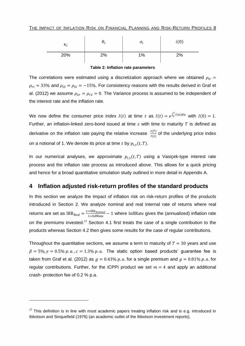
20% 2% 1% 2%

Table 2: Inflation rate parameters

The correlations were estimated using a discretization approach where we obtained

and . For consistency reasons with the results derived in Graf et

al. (2012) we assume . The Variance process is assumed to be independent of

the interest rate and the inflation rate.

We now define the consumer price index at time as

with .

Further, an inflation-linked zero-bond issued at time with time to maturity is defined as

derivative on the inflation rate paying the relative increase

of the underlying price index

on a notional of 1. We denote its price at time by .

In our numerical analyses, we approximate using a Vasiçek-type interest rate

process and the inflation rate process as introduced above. This allows for a quick pricing

and hence for a broad quantitative simulation study outlined in more detail in Appendix A.

4 Inflation adjusted risk-return profiles of the standard products

In this section we analyze the impact of inflation risk on risk-return profiles of the products

introduced in Section 2. We analyze nominal and real internal rate of returns where real

returns are set as

where gives the (annualized) inflation rate

on the premiums invested.17 Section 4.1 first treats the case of a single contribution to the

products whereas Section 4.2 then gives some results for the case of regular contributions.

Throughout the quantitative sections, we assume a term to maturity of years and use

The static option based products’ guarantee fee is

taken from Graf et al. (2012) as for a single premium and for

regular contributions. Further, for the iCPPI product we set and apply an additional

crash- protection fee of 0.2 % p.a.

17 This definition is in line with most academic papers treating inflation risk and is e.g. introduced in

Ibbotson and Sinquefield (1976) (an academic outlet of the Ibbotson investment reports).


4.1 Single contribution

We start with analyzing a single contribution to the products introduced in Section 2. Figure 1

gives the empirical frequency distributions of internal rates of return applying 50,000

trajectories.

Figure 1: Empirical nominal (upper) and real (lower) rates of return - single contribution

0%

2%

4%

6%

8%

10%

12%

14%

16%

18%

20%

-12% -10% -8% -6% -4% -2% 0% 2% 4% 6% 8% 10% 12%

Frequency distribution (nominal returns)

NominalZero Bond

Zero + Underlying Option Based Product

iCPPI Equity Fund

0%

2%

4%

6%

8%

10%

12%

14%

16%

18%

20%

-12% -10% -8% -6% -4% -2% 0% 2% 4% 6% 8% 10% 12%

Frequency distribution (real returns)

NominalZero Bond

Zero + Underlying Option Based Product

iCPPI Equity Fund


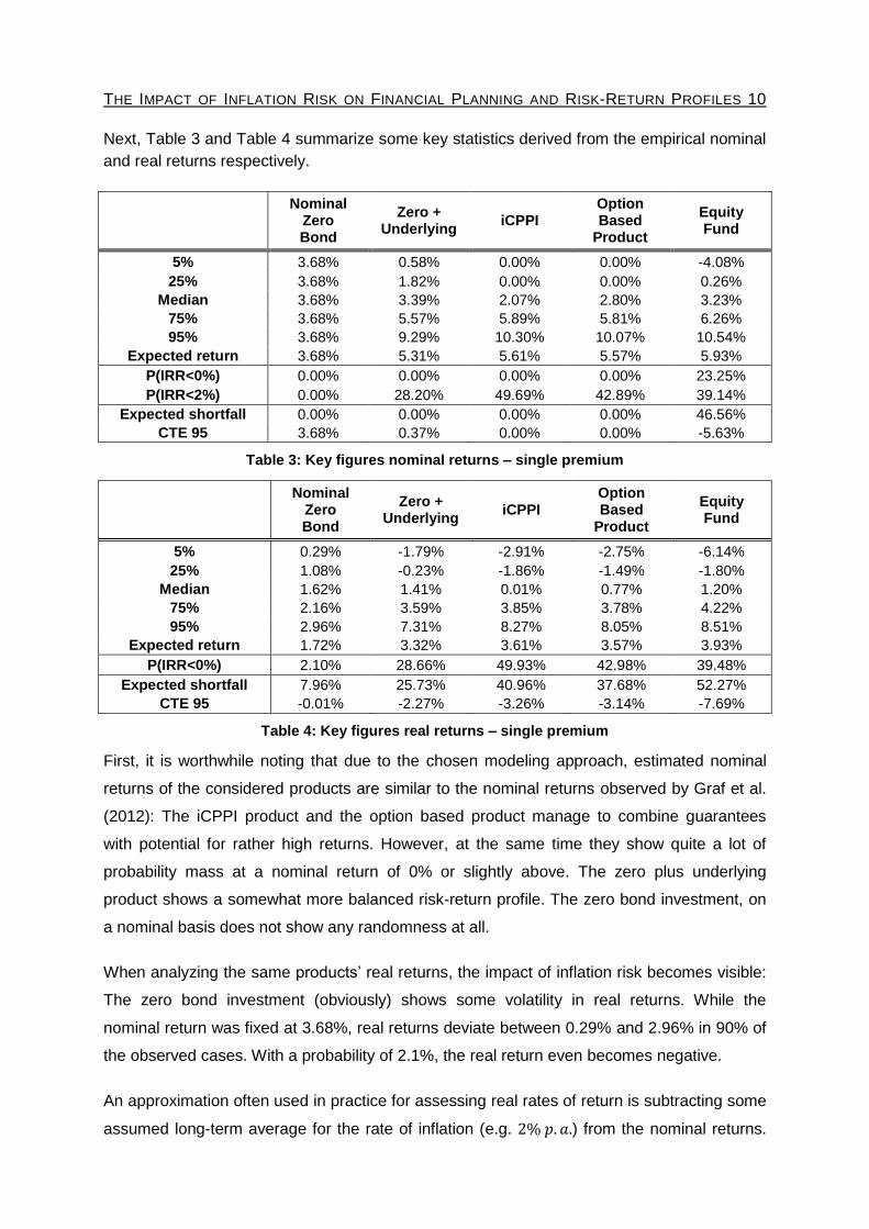
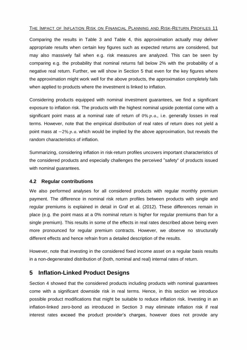
Next, Table 3 and Table 4 summarize some key statistics derived from the empirical nominal

and real returns respectively.

Nominal Zero Bond

Zero + Underlying

iCPPI Option Based

Product

Equity Fund

5% 3.68% 0.58% 0.00% 0.00% -4.08%

25% 3.68% 1.82% 0.00% 0.00% 0.26%

Median 3.68% 3.39% 2.07% 2.80% 3.23%

75% 3.68% 5.57% 5.89% 5.81% 6.26%

95% 3.68% 9.29% 10.30% 10.07% 10.54%

Expected return 3.68% 5.31% 5.61% 5.57% 5.93%

P(IRR<0%) 0.00% 0.00% 0.00% 0.00% 23.25%

P(IRR<2%) 0.00% 28.20% 49.69% 42.89% 39.14%

Expected shortfall 0.00% 0.00% 0.00% 0.00% 46.56%

CTE 95 3.68% 0.37% 0.00% 0.00% -5.63%

Table 3: Key figures nominal returns – single premium

Nominal Zero Bond

Zero + Underlying

iCPPI Option Based

Product

Equity Fund

5% 0.29% -1.79% -2.91% -2.75% -6.14%

25% 1.08% -0.23% -1.86% -1.49% -1.80%

Median 1.62% 1.41% 0.01% 0.77% 1.20%

75% 2.16% 3.59% 3.85% 3.78% 4.22%

95% 2.96% 7.31% 8.27% 8.05% 8.51%

Expected return 1.72% 3.32% 3.61% 3.57% 3.93%

P(IRR<0%) 2.10% 28.66% 49.93% 42.98% 39.48%

Expected shortfall 7.96% 25.73% 40.96% 37.68% 52.27%

CTE 95 -0.01% -2.27% -3.26% -3.14% -7.69%

Table 4: Key figures real returns – single premium

First, it is worthwhile noting that due to the chosen modeling approach, estimated nominal

returns of the considered products are similar to the nominal returns observed by Graf et al.

(2012): The iCPPI product and the option based product manage to combine guarantees

with potential for rather high returns. However, at the same time they show quite a lot of

probability mass at a nominal return of 0% or slightly above. The zero plus underlying

product shows a somewhat more balanced risk-return profile. The zero bond investment, on

a nominal basis does not show any randomness at all.

When analyzing the same products’ real returns, the impact of inflation risk becomes visible:

The zero bond investment (obviously) shows some volatility in real returns. While the

nominal return was fixed at 3.68%, real returns deviate between 0.29% and 2.96% in 90% of

the observed cases. With a probability of 2.1%, the real return even becomes negative.

An approximation often used in practice for assessing real rates of return is subtracting some

assumed long-term average for the rate of inflation (e.g. ) from the nominal returns.


Comparing the results in Table 3 and Table 4, this approximation actually may deliver

appropriate results when certain key figures such as expected returns are considered, but

may also massively fail when e.g. risk measures are analyzed. This can be seen by

comparing e.g. the probability that nominal returns fall below 2% with the probability of a

negative real return. Further, we will show in Section 5 that even for the key figures where

the approximation might work well for the above products, the approximation completely fails

when applied to products where the investment is linked to inflation.

Considering products equipped with nominal investment guarantees, we find a significant

exposure to inflation risk. The products with the highest nominal upside potential come with a

significant point mass at a nominal rate of return of , i.e. generally losses in real

terms. However, note that the empirical distribution of real rates of return does not yield a

point mass at which would be implied by the above approximation, but reveals the

random characteristics of inflation.

Summarizing, considering inflation in risk-return profiles uncovers important characteristics of

the considered products and especially challenges the perceived ”safety“ of products issued

with nominal guarantees.

4.2 Regular contributions

We also performed analyses for all considered products with regular monthly premium

payment. The difference in nominal risk return profiles between products with single and

regular premiums is explained in detail in Graf et al. (2012). These differences remain in

place (e.g. the point mass at a 0% nominal return is higher for regular premiums than for a

single premium). This results in some of the effects in real rates described above being even

more pronounced for regular premium contracts. However, we observe no structurally

different effects and hence refrain from a detailed description of the results.

However, note that investing in the considered fixed income asset on a regular basis results

in a non-degenerated distribution of (both, nominal and real) internal rates of return.

5 Inflation-Linked Product Designs

Section 4 showed that the considered products including products with nominal guarantees

come with a significant downside risk in real terms. Hence, in this section we introduce

possible product modifications that might be suitable to reduce inflation risk. Investing in an

inflation-linked zero-bond as introduced in Section 3 may eliminate inflation risk if real

interest rates exceed the product provider’s charges, however does not provide any


additional upside potential. Nevertheless, we include this type of investment in the following

analyses.

Corrigan et al. (2011) propose ideas on issuing “Variable Annuity type” guarantees providing

inflation risk protection by some form of an additional option on the mutual fund investment

as introduced above. Further, they derive fair (i.e. risk-neutral) prices of these types of

guarantees. Their results indicate that a complete option-based inflation risk protection may

come at a rather high cost. Hence, full coverage of inflation risk by means of an option

seems very expensive resulting in products with rather limited upside potential. To the best of

our knowledge no research has been done with respect to modifying the products introduced

above in order to cope with inflation risk. However, Fulli-Lemaire (2012) introduce some

hybrid trading strategy taking into account inflation estimates and analyze their potential

using historical backtesting and block bootstrapping techniques.

In what follows, we focus on modifying the iCPPI and the zero plus underlying products in

order to provide some reduction (not necessarily a complete elimination) of inflation risk. Our

modifications are based on two basic ideas: 1) incorporating some estimate for future

inflation in the guarantee basis which then impacts the calculation of the floor and hence

results in a different asset allocation as compared to the original products and 2) using a

different asset than nominal zero-bonds as a “risk-free asset”, e.g. an inflation-linked zero-

bond, and calculate the floor accordingly (see below). Similar to Section 2, we state the

necessary formulae for both single and regular contributions, however concentrate on

quantitative analyses of a single contribution and only briefly comment on the results for

regular contributions where additional insights are gained.

Note that vis-a-vis the client, the modified products come without any nominal or real

investment guarantee. Nevertheless, we still use the terms guarantee basis and floor as

introduced in Section 2.

5.1 Modification of the nominal guarantee basis

Our first approach is a modification of the nominal guarantee basis by allowing for

inflation. At time the modified guarantee basis consists of the realized inflation on the

premiums until time (which is a -measurable random variable determined by as

introduced in Section 3) and some estimate for the future rate of inflation within .

We set

when a single premium is considered and


when regular contributions are in place.

We consider two different approaches for estimating : In the historic approach, we use

the realized rate of inflation until time as an estimate for the future rate of inflation as well.

In the market approach, we use the market’s expectation on the future rate of inflation until

maturity .

In the historic approach we obviously obtain

for the single premium case

and

in the regular premium case where gives

the internal rate of return of a vector of contributions and a corresponding benefit .

In the market approach, we instead use the market’s expectation on the future rate of

inflation implied by inflation-linked derivatives (e.g. inflation-linked bonds or inflation swaps).

According to Corrigan et al. (2011) and e.g. a report by Kerkhof (2005), the market for zero-

coupon inflation swaps is amongst the most liquid inflation-linked derivatives markets. In our

model setup, the inflation swap issued at time delivers the relative increase

at maturity

against the fixed rate on a notional of 1. No arbitrage arguments then yield (cf. e.g.

Mercurio (2005)) the fair swap rate to fulfil

.18 Hence, the fair swap rate

is (without any model assumption) uniquely determined by the prices of nominal and

inflation-linked zero-bonds. Further note that the swap rate in general not only shows the

market’s expectation for the future rate of inflation but also includes various additional risk

premiums such as e.g. liquidity or credit risk. Hence, these additional risk premiums may be

filtered out to obtain a “best estimate” of the market’s inflation expectation as e.g. done in

Schulz and Stapf (2009). Since we do not model any additional risk factors, we extract the

market’s inflation expectation directly from and set .19

Of course, the historic approach is easier implemented in practice, since no additional data is

required. However, if significant changes in the (future) rate of inflation occur, e.g. due to a

18 Note, the swap rate is usually directly quoted by brokers, e.g. on Bloomberg.

19 Within the Appendix we show how prices of the inflation-linked zero-bond are computed in

our work and how we are hence able to derive an estimate for .


change in the monetary policy, the historic approach only reacts with a certain time-lag

whereas the market approach should be able to pick up this change rather quickly.

Based on the modified guarantee basis, the allocation mechanisms for the iCPPI and the

zero plus underlying remain unchanged as described in Section 2. In particular, in this

approach, the products still use nominal zero-bonds as riskless assets.

5.2 Use of inflation-linked zero-bonds instead of nominal zero-bonds

Neglecting liquidity issues that may arise in a practical application, in our second approach,

we use inflation-linked bonds as “safe assets” in the iCPPI and zero plus underlying products

introduced in Section 2. For ease of notation, we assume that the product provider solely

invests in the inflation-linked zero-bond issued at time 0.

Similar with Section 2, let denote the guarantee base at time . However, here we identify

as the number of units that have to be invested in the considered inflation-linked zero-

bond in order to provide the inflation protection for the invested premium(s). If a premium is

contributed to the contract at time ,

units of above inflation-linked zero-bond deliver

which exactly gives the premium after

allowing for inflation. Hence, we set

for single premium contracts. For

regular premium contracts, we set

and

at every monthly

premium payment date . The floor is consequently calculated as

. The

asset allocation of the zero plus underlying and the iCPPI products then follow exactly the

formulae introduced in Section 2, but using the floor introduced in this section and the

inflation-linked zero-bond as riskless asset.

Note, that this product is somehow similar to the product introduced in Section 5.1 applying a

market-based approach, since we obtain

when a single contribution is considered. Similar derivations are possible for regular

contributions. Hence, both products allocate the same amount of (nominal) money into the

riskless asset but assume a different riskless asset.


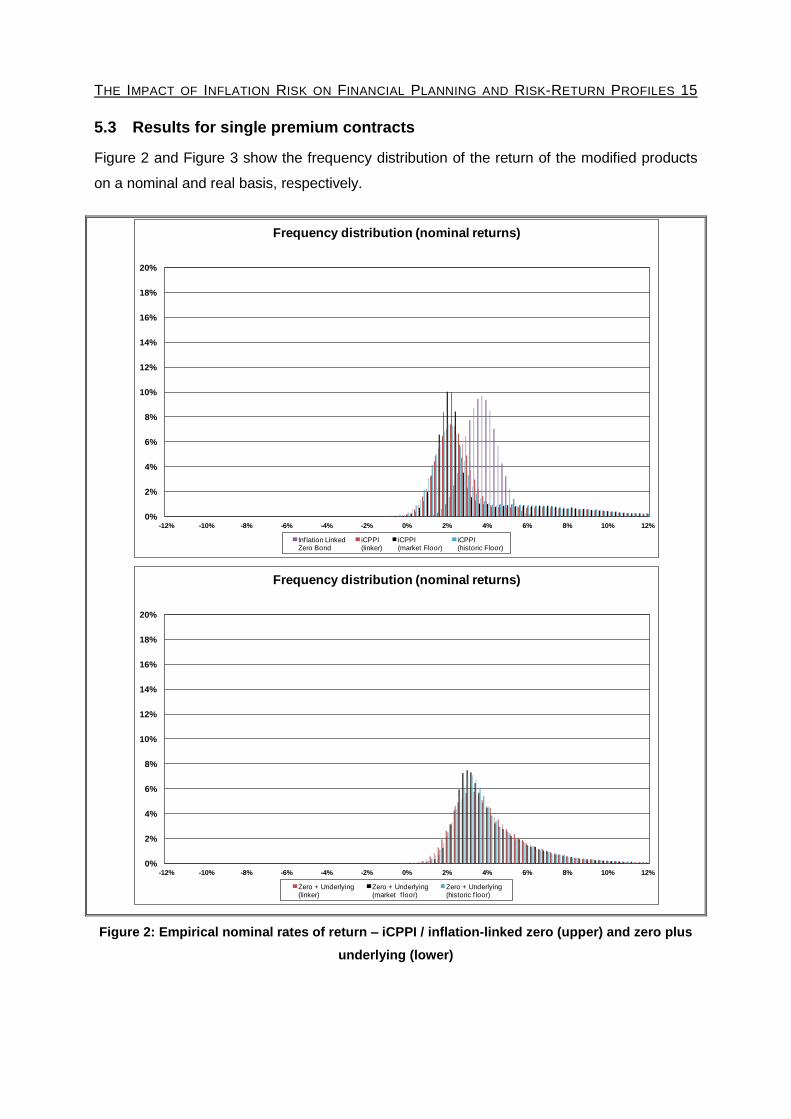
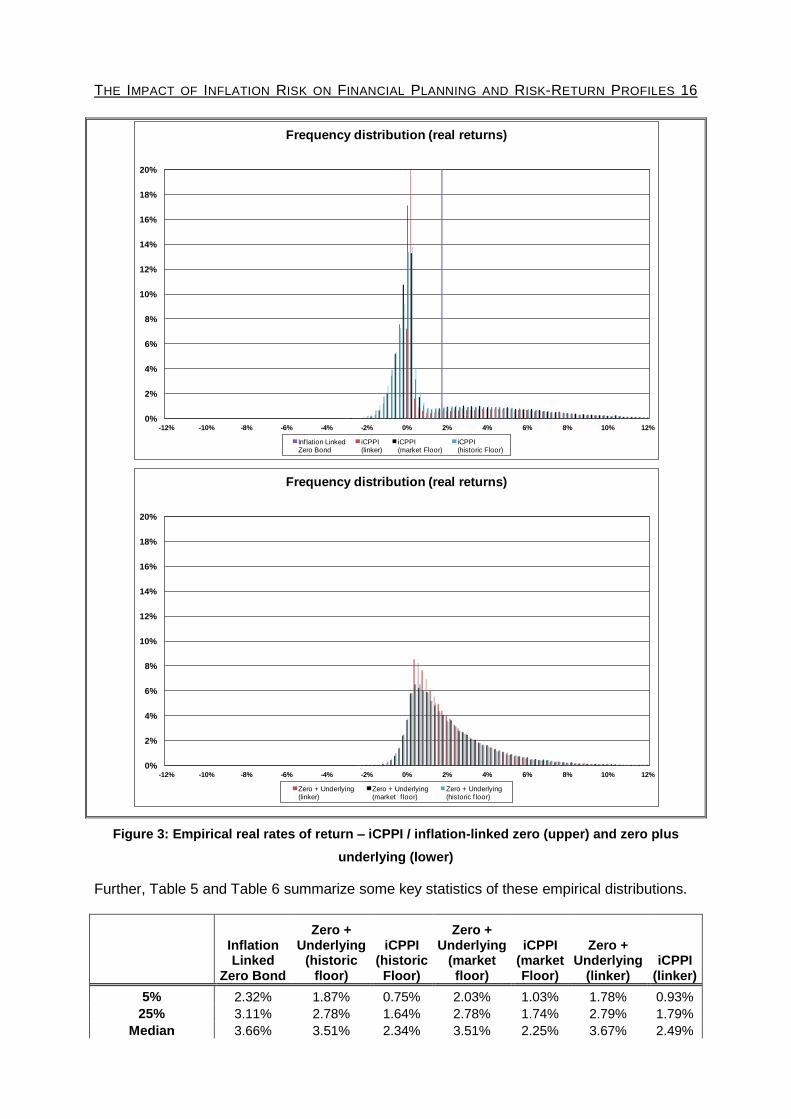
5.3 Results for single premium contracts

Figure 2 and Figure 3 show the frequency distribution of the return of the modified products

on a nominal and real basis, respectively.

Figure 2: Empirical nominal rates of return – iCPPI / inflation-linked zero (upper) and zero plus

underlying (lower)

0%

2%

4%

6%

8%

10%

12%

14%

16%

18%

20%

-12% -10% -8% -6% -4% -2% 0% 2% 4% 6% 8% 10% 12%


Inf lation Linked Zero Bond

iCPPI (linker)

iCPPI (market Floor)

iCPPI (historic Floor)

0%

2%

4%

6%

8%

10%

12%

14%

16%

18%

20%

-12% -10% -8% -6% -4% -2% 0% 2% 4% 6% 8% 10% 12%


Zero + Underlying (linker)

Zero + Underlying (market f loor)

Zero + Underlying (historic f loor)


Figure 3: Empirical real rates of return – iCPPI / inflation-linked zero (upper) and zero plus

underlying (lower)

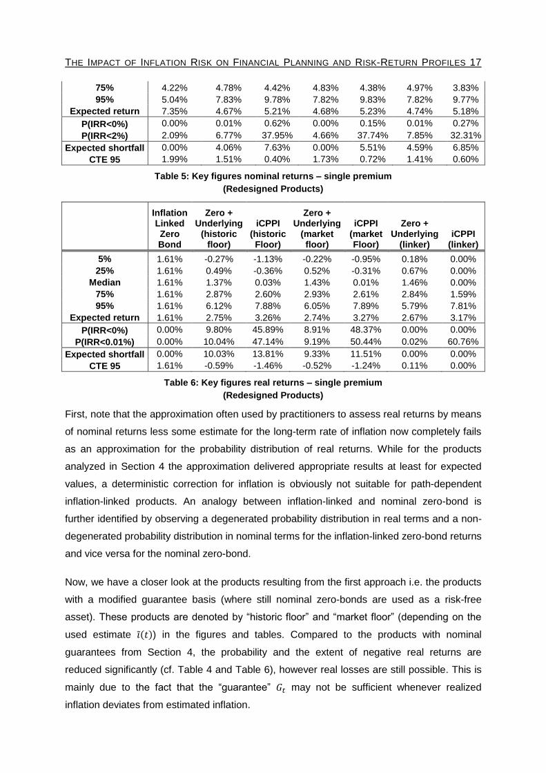
Further, Table 5 and Table 6 summarize some key statistics of these empirical distributions.

Inflation Linked

Zero Bond

Zero + Underlying

(historic floor)


Zero + Underlying

(market floor)


Zero + Underlying

(linker) iCPPI

(linker)

5% 2.32% 1.87% 0.75% 2.03% 1.03% 1.78% 0.93%

25% 3.11% 2.78% 1.64% 2.78% 1.74% 2.79% 1.79%

Median 3.66% 3.51% 2.34% 3.51% 2.25% 3.67% 2.49%

0%

2%

4%

6%

8%

10%

12%

14%

16%

18%

20%

-12% -10% -8% -6% -4% -2% 0% 2% 4% 6% 8% 10% 12%


Inf lation Linked Zero Bond

iCPPI (linker)



0%

2%

4%

6%

8%

10%

12%

14%

16%

18%

20%

-12% -10% -8% -6% -4% -2% 0% 2% 4% 6% 8% 10% 12%


Zero + Underlying (linker)

Zero + Underlying (market f loor)

Zero + Underlying (historic f loor)


75% 4.22% 4.78% 4.42% 4.83% 4.38% 4.97% 3.83%

95% 5.04% 7.83% 9.78% 7.82% 9.83% 7.82% 9.77%

Expected return 7.35% 4.67% 5.21% 4.68% 5.23% 4.74% 5.18%

P(IRR<0%) 0.00% 0.01% 0.62% 0.00% 0.15% 0.01% 0.27%

P(IRR<2%) 2.09% 6.77% 37.95% 4.66% 37.74% 7.85% 32.31%

Expected shortfall 0.00% 4.06% 7.63% 0.00% 5.51% 4.59% 6.85%

CTE 95 1.99% 1.51% 0.40% 1.73% 0.72% 1.41% 0.60%

Table 5: Key figures nominal returns – single premium

(Redesigned Products)

Inflation Linked Zero Bond

Zero + Underlying

(historic floor)


Zero + Underlying

(market floor)


Zero + Underlying

(linker) iCPPI

(linker)

5% 1.61% -0.27% -1.13% -0.22% -0.95% 0.18% 0.00%

25% 1.61% 0.49% -0.36% 0.52% -0.31% 0.67% 0.00%

Median 1.61% 1.37% 0.03% 1.43% 0.01% 1.46% 0.00%

75% 1.61% 2.87% 2.60% 2.93% 2.61% 2.84% 1.59%

95% 1.61% 6.12% 7.88% 6.05% 7.89% 5.79% 7.81%

Expected return 1.61% 2.75% 3.26% 2.74% 3.27% 2.67% 3.17%

P(IRR<0%) 0.00% 9.80% 45.89% 8.91% 48.37% 0.00% 0.00%

P(IRR<0.01%) 0.00% 10.04% 47.14% 9.19% 50.44% 0.02% 60.76%

Expected shortfall 0.00% 10.03% 13.81% 9.33% 11.51% 0.00% 0.00%

CTE 95 1.61% -0.59% -1.46% -0.52% -1.24% 0.11% 0.00%

Table 6: Key figures real returns – single premium


First, note that the approximation often used by practitioners to assess real returns by means

of nominal returns less some estimate for the long-term rate of inflation now completely fails

as an approximation for the probability distribution of real returns. While for the products

analyzed in Section 4 the approximation delivered appropriate results at least for expected

values, a deterministic correction for inflation is obviously not suitable for path-dependent

inflation-linked products. An analogy between inflation-linked and nominal zero-bond is

further identified by observing a degenerated probability distribution in real terms and a non-

degenerated probability distribution in nominal terms for the inflation-linked zero-bond returns

and vice versa for the nominal zero-bond.

Now, we have a closer look at the products resulting from the first approach i.e. the products

with a modified guarantee basis (where still nominal zero-bonds are used as a risk-free

asset). These products are denoted by “historic floor” and “market floor” (depending on the

used estimate ) in the figures and tables. Compared to the products with nominal

guarantees from Section 4, the probability and the extent of negative real returns are

reduced significantly (cf. Table 4 and Table 6), however real losses are still possible. This is

mainly due to the fact that the “guarantee” may not be sufficient whenever realized

inflation deviates from estimated inflation.


Comparing the historic and market approach, we find that the market approach may deliver

better results than the historic approach especially when lower percentiles of the real returns’

distributions are used as a risk measure. Hence, the extent of real losses (if they occur) is

generally lower when a market based approach is implemented instead of a pure historic

estimate, since the market based approach generally picks up changes in the future rate of

inflation more quickly than the historic approach does.20

We now look at the second approach for modification, i.e. products where inflation-linked

zero-bonds instead of nominal zero-bonds are used as a safe asset. These two products are

denoted by “linker” in the figures and tables. Although nominal losses are possible (cf. Table

5), the risk of negative real returns is significantly reduced: Considering the zero plus

underlying product, there is no risk of negative real returns in the single premium case21

whereas for the iCPPI product, real losses are possible due to gap events which are however

not observed in our simulation study. Further, the probability distributions of real rates for the

modified products and the corresponding probability distributions of nominal rates for the

“standard” products (cf. Figure 1 and Figure 2) have a similar shape.

Both products still offer some upside potential. Clearly, the iCPPI product comes with more

fluctuation compared to the zero plus underlying product. In the 95th percentile, for example,

the iCPPI versions even under real returns achieve an IRR of almost 8%. However the cost

of providing a very high upside potential in good capital market scenarios goes hand in hand

with a very high probability of approximately 60% of “just” getting the inflated premiums back.

In contrast, the zero plus underlying delivers a more moderate distribution of real returns

which results in less upside potential but also a lower probability of very low or even zero real

returns. Hence, considering these products and products ‘in between these two products’

seems a promising way of creating different inflation-protected products for clients with

different degrees of risk aversion.

Finally note that, although in our simulation study no negative real returns were observed,

there is no guarantee embedded in the products. If e.g. a massive increase in the expected

future rate of inflation (and thus massive increase in the inflation-linked zero-bonds’ price)

occurs simultaneously with a dramatic loss in equity, especially the introduced iCPPI product

may not be able to buy the required inflation-linked zero-bonds after that event and hence

real losses are possible.

20 In a model with “regime switches” in the monetary policy this effect might even be more pronounced.

21 Obviously this only holds if .


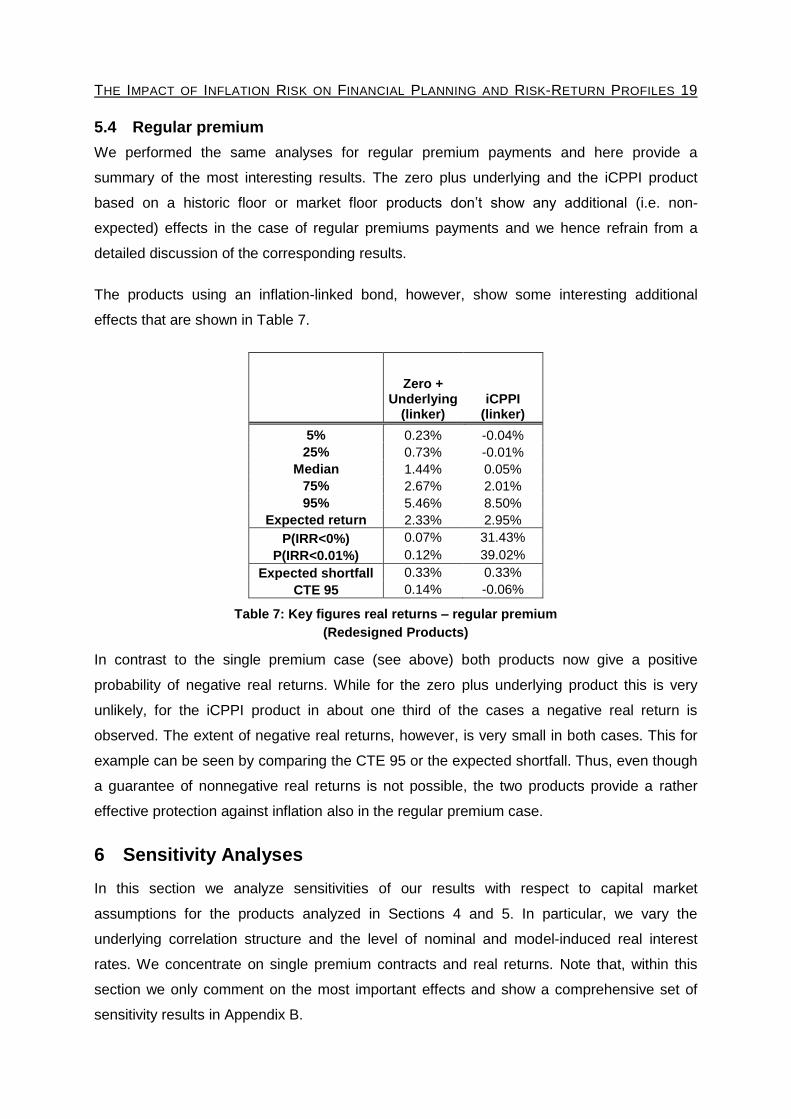
5.4 Regular premium

We performed the same analyses for regular premium payments and here provide a

summary of the most interesting results. The zero plus underlying and the iCPPI product

based on a historic floor or market floor products don’t show any additional (i.e. non-

expected) effects in the case of regular premiums payments and we hence refrain from a

detailed discussion of the corresponding results.

The products using an inflation-linked bond, however, show some interesting additional

effects that are shown in Table 7.

Zero + Underlying

(linker) iCPPI

(linker)

5% 0.23% -0.04%

25% 0.73% -0.01%

Median 1.44% 0.05%

75% 2.67% 2.01%

95% 5.46% 8.50%

Expected return 2.33% 2.95%

P(IRR<0%) 0.07% 31.43%

P(IRR<0.01%) 0.12% 39.02%

Expected shortfall 0.33% 0.33%

CTE 95 0.14% -0.06%

Table 7: Key figures real returns – regular premium


In contrast to the single premium case (see above) both products now give a positive

probability of negative real returns. While for the zero plus underlying product this is very

unlikely, for the iCPPI product in about one third of the cases a negative real return is

observed. The extent of negative real returns, however, is very small in both cases. This for

example can be seen by comparing the CTE 95 or the expected shortfall. Thus, even though

a guarantee of nonnegative real returns is not possible, the two products provide a rather

effective protection against inflation also in the regular premium case.

6 Sensitivity Analyses

In this section we analyze sensitivities of our results with respect to capital market

assumptions for the products analyzed in Sections 4 and 5. In particular, we vary the

underlying correlation structure and the level of nominal and model-induced real interest

rates. We concentrate on single premium contracts and real returns. Note that, within this

section we only comment on the most important effects and show a comprehensive set of

sensitivity results in Appendix B.


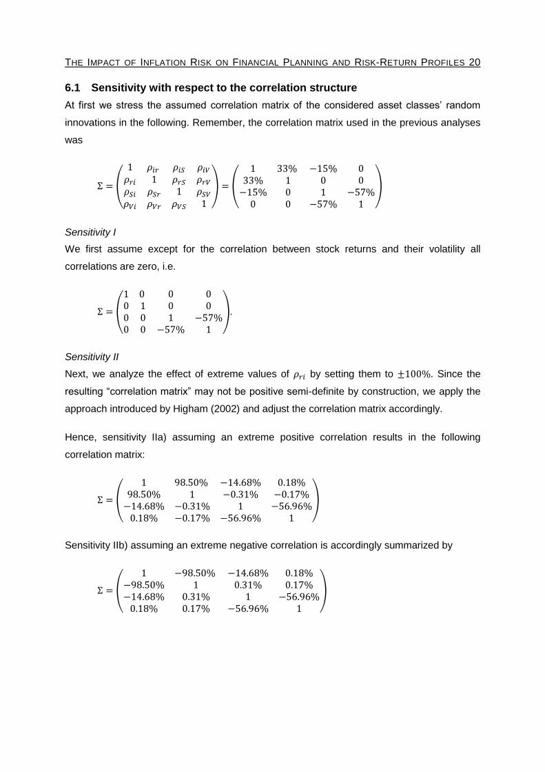
6.1 Sensitivity with respect to the correlation structure

At first we stress the assumed correlation matrix of the considered asset classes’ random

innovations in the following. Remember, the correlation matrix used in the previous analyses

was

Sensitivity I

We first assume except for the correlation between stock returns and their volatility all

correlations are zero, i.e.

.

Sensitivity II

Next, we analyze the effect of extreme values of by setting them to . Since the

resulting “correlation matrix” may not be positive semi-definite by construction, we apply the

approach introduced by Higham (2002) and adjust the correlation matrix accordingly.

Hence, sensitivity IIa) assuming an extreme positive correlation results in the following

correlation matrix:

Sensitivity IIb) assuming an extreme negative correlation is accordingly summarized by


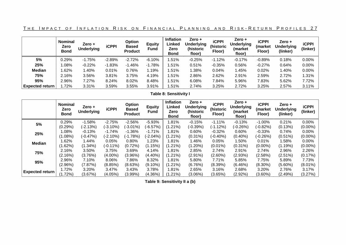
Results:

First note that the distribution of real investment returns remains unchanged for the nominal

zero-bond.22 Further, Table 8 in Appendix B shows that the assumption of a zero correlation

does not change the results too much and hence we only comment on the extreme positive

and negative correlation assumptions in the following.

The equity fund investment and the option based product provide a pure investment in the

considered equity process whose performance is influenced by the interest rates and hence

due to the correlation also related to the rate of inflation. We observe that when a positive

correlation of interest rates and the rate of inflation is assumed, the products’ lower

respectively upper tails (roughly approximated by the 5th and 95th percentile) increase and

decrease respectively, i.e. we observe less variability. For a negative correlation, we observe

the opposite effect. A similar effect occurs with the considered hybrid products, on the one

side due to the same effect in the equity part and on the other side due to the fact that when

the inflation rate increases, the product’s floor – as a function of the considered interest rates

– potentially decreases (increases) when correlation is positive (negative) (cf. Table 9)

leaving the products with higher (lower) equity share.

For the modified products as introduced in Section 5, it is worthwhile noting that, although the

payout of the inflation-linked zero-bond does not change, we observe a different deterministic

real return of the considered investment product when compared to the base-case. This is

due to the inflation-linked bond’s different price at . Further, the modified guarantee

products are generally more “volatile” when negative correlations of interest rates and

inflation rates are assumed, leaving the products with a potentially higher upside at the cost

of a more pronounced downside as well (cf. Table 9).

6.2 Sensitivity with respect to the level of nominal interest rates and rate of

inflation

We now stress the level of nominal interest rates and inflation by analyzing the following

sensitivities. Again, all other assumptions remain unchanged, in particular the “base case”

correlation matrix as introduced in Section 3 is applied.

22 Note, this effect is only observed for a single contribution and changes when regular contributions

are in place.


Sensitivity III

We assume an increase (decrease) of both, the start level and the long term average of

interest rates and inflation, i.e. in sensitivity IIIa) and

in sensitivity IIIb).

Results:

Since in this sensitivity analysis, the level of interest rates and inflation is stressed by the

same amount, the level of real rates remains more or less unchanged. Therefore, the real

probability distributions of non-hybrid standard products (i.e. pure equity and fixed income

investment) are very similar to the base case. However, when considering hybrid products,

this observation changes (tremendously). When the level of interest rates is increased

(decreased), the equity exposure of the considered products increases (decreases) as well

which generally generates more (less) volatility in the products. Further, from a real point of

view, the nominal guarantee’s value decreases (increases) when the level of inflation

increases (decreases). These effects therefore increase the product’s downside (in terms of

real returns) even when interest rates are higher (cf. Table 10).

In contrast, the modified products as introduced in Section 5 are generally only influenced by

the level of real interest rates and hence their probability distributions remain largely

unchanged when sensitivity III is applied (cf. Table 10) when real rates stay at a similar level.

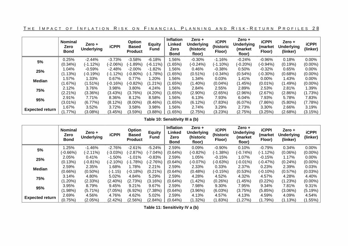
Sensitivity IV

Finally we investigate an increase (decrease) of the level of real interest rates by 1% by

assuming in sensitivity IVa) and in sensitivity IVb) while

leaving unchanged.

Results:

When real rates increase (decrease) the effects on the standard products are exactly as

expected: We observe a positive (negative) shift of the resulting return distributions (cf. Table

11). Increasing the level of real interest rates decreases the price of an inflation-linked zero-

bond and hence increases the cushion of all considered modified guarantee products (and

vice versa). Therefore, the results for these products are (obviously) worse when real interest

rates tend to be low. Additionally, path-dependant products suffer more than path-

independent products since the former essentially result in very skewed return distributions

(cf. Table 11).


7 Conclusion and Outlook

This paper shows the impact of inflation risk on the risk-return profiles of various old age

provision products. After extending the model introduced in Graf et al. (2012) by taking

inflation risk into account we derived the risk-return profiles for various common standard old

age provision products assuming e.g. different portfolio insurance strategies. We found that

most products – including products that are often considered particularly safe by practitioners

and regulators due to nominal guarantees – bear a significant inflation risk and especially

found that information about a product’s return distribution in real terms (that is not revealed

by information provided to clients and their financial advisors so far) is relevant for

sustainable financial planning. Finally, we have proposed product modifications that may

reduce or even remove the risk of negative real investment returns while still allowing for

some upside potential.

Of course, this work is only a first starting point in this area of research. Future research

could include an assessment of model risk, in particular taking into account the impact of the

recent monetary policy by the various central banks due to the debt crisis. Further, it seems

worthwhile studying whether the inflation-linked derivatives market is liquid enough for

institutional investors to actually implement the proposed product modifications in practice.

References

Ahlgrim K. C., D’Arcy S. P. and Gorvett R. W. (2005): Modeling Financial Scenarios: A

Framework for Actuarial Profession. Proceedings of the Casualty Actuarial Society 92:

177–238.

Amenc N., Martellini L. and Ziemann V. (2009). Alternative Investments for Institutional

Investors, Risk Budgeting Techniques in Asset Management and Asset-Liability

Management. The Journal of Portfolio Management, 35(4): 94-110.

Beletski T. and Korn R. (2006): Optimal Investment with Inflation-linked Products. Advances

in Risk Management Palgrave-Mac Millan: 170-190.

Belgrade N., Benhamou E. and Koehler E. (2004): A market model for inflation. CDC Ixis

Capital Markets. Available at SSRN http://ssrn.com/abstract=576081.

Black F. and Perold A. F. (1992). Theory of constant proportion portfolio. Journal of

Economic Dynamics and Control, 16 (3-4):403-426.

Corrigan J., De Weirdt M., Fang F. and Lockwodd D. (2011). Manufacturing Inflation Risk

Protection. Institute of Actuaries of Australia.

http://ssrn.com/abstract=576081


Cox J. C., Ingersoll J. E. and Ross S. A. (1985). A Theory of the Term Structure of Interest

Rates. Econometrica, 53(2):385-407.

Fulli-Lemaire N. (2012). A Dynamic Inflation Hedging Trading Strategy Using a CPPI.

Available at SSRN: http://ssrn.com/abstract=1978438.

Graf S., Kling A. and Ruß J. (2012) Financial Planning and Risk-Return Profiles. European

Actuarial Journal, 2(1):77-104.

Heston S. L. (1993). A Closed-Form Solution for Options with Stochastic Volatility with

Applications to Bond and Currency Options. The Review of Financial Studies, 6(2):327-

343.

Higham N. J. (2002). Computing the nearest correlation matrix – a problem from finance.

IMA Journal of Numerical Analysis, 22: 329-343.

Ibbotson R. G. and Sinquefield R. A. (1976). Stocks, Bonds, Bills, and Inflation: Year-by-

Year Historical Returns (1926-1974). The Journal of Business, 49(1): pp. 11-47.

Jarrow, R. and Yildirim, Y. (2003). Pricing Treasury Inflation Protected Securities and

Related Derivatives using an HJM Model, Journal of Financial and Quantitative Analysis,

38(2): 337-358.

Kerkhof J. (2005). Inflation Derivatives Explained Markets, Products, and Pricing. Fixed

Income Quantitative Research Lehmann Brothers. Available at:

http://www.scribd.com/doc/86770535/19601807-Lehman-Brothers-Kerkhof-Inflation-

Derivatives-Explained-Markets-Products-and-Pricing.

Mercurio F. (2005). Pricing inflation-indexed derivatives. Quantitative Finance, 5(3):289-301.

Schulz A. and Stapf J. (2009). Price discovery on traded inflation expectations: Does the

financial crisis matter? Deutsche Bundesbank Disussion Paper Series 1: Economic

Studies No 25/2009.

Sørensen M. (1997), Estimating Functions for Discretely Observed Diffusions: A Review.

Lecture Notes-Monograph Series, 32, 305-325.

Tankov P. (2010). Pricing and hedging gap risk. The Journal of Computational Finance,

13(3).

Vasiçek O. (1977). An Equilibrium Characterization of the Term Structure. Journal of

Financial Economics, 5: 177-188.

http://ssrn.com/abstract=1978438

http://www.scribd.com/doc/86770535/19601807-Lehman-Brothers-Kerkhof-Inflation-Derivatives-Explained-Markets-Products-and-Pricing

http://www.scribd.com/doc/86770535/19601807-Lehman-Brothers-Kerkhof-Inflation-Derivatives-Explained-Markets-Products-and-Pricing


A Pricing of inflation-linked zero-bonds

In this section we briefly sketch the implemented pricing of inflation-linked zero-bonds used

in the products in Section 5. Note that in the considered asset model introduced in Section 3

nominal interest rates follow a Cox-Ingersoll-Ross model and rates of inflation follow a

Vasiçek model. To the best of our knowledge, no closed form solution for pricing inflation-

linked zero-bonds is available in this setup. Hence, we assume the following approximation

for pricing:23 We assume the rate of inflation and the nominal interest rates to follow

correlated Vasiçek processes:

with . This model is “consistent” with the original model (cf. Section 3) if

we set , and . By no-arbitrage arguments, the price at time t of an

inflation-linked zero-bond issued at time with time-to-maturity is then

derived as

Since

and

follow a normal distribution,

and

are

normally distributed as well. Hence, the price is finally computed as the expectation

of a log-normal distributed random variable.

We now briefly sketch the (not complicated though rather tedious) derivation of the

distribution of

which is derived from the joint multivariate normal

distribution of

which is itself completely determined by the

expectation, variance and covariance of

and

respectively.

23 This approximation may also be identified as incorporating some model risk in our analyses when

inflation-linked derivatives are priced.


Expectation and variance of the processes are derived using the identity

for and the fact that

.

Finally, the covariance of the considered processes is calculated as follows

which can then be computed analytically as well.

B Sensitivity Analyses – Results

This section gives details with respect to the results explained in Section 6. We display key

statistics of the observed real returns considering a single premium investment only.

T H E I M P A C T O F I N F L A T I O N R I S K O N F I N A N C I A L P L A N N I N G A N D R I S K - R E T U R N P R O F I L E S 2 7

Nominal Zero Bond

Zero + Underlying

iCPPI Option Based

Product

Equity Fund


Zero + Underlying

(historic floor)


Zero + Underlying

(market floor)


Zero + Underlying

(linker)

iCPPI (linker)

5% 0.29% -1.75% -2.89% -2.72% -6.10% 1.51% -0.25% -1.12% -0.17% -0.89% 0.18% 0.00%

25% 1.08% -0.22% -1.83% -1.46% -1.78% 1.51% 0.51% -0.35% 0.56% -0.27% 0.64% 0.00%

Median 1.62% 1.40% 0.01% 0.76% 1.19% 1.51% 1.38% 0.04% 1.45% 0.02% 1.40% 0.00%

75% 2.16% 3.56% 3.81% 3.75% 4.19% 1.51% 2.86% 2.62% 2.91% 2.59% 2.72% 1.31%

95% 2.96% 7.27% 8.24% 8.02% 8.48% 1.51% 6.08% 7.84% 5.96% 7.83% 5.62% 7.72%

Expected return 1.72% 3.31% 3.59% 3.55% 3.91% 1.51% 2.74% 3.25% 2.72% 3.25% 2.57% 3.11%

Table 8: Sensitivity I

Nominal Zero Bond

Zero + Underlying

iCPPI Option Based

Product

Equity Fund


Zero + Underlying

(historic floor)


Zero + Underlying

(market floor)


Zero + Underlying

(linker)

iCPPI (linker)

5% 0.29%

(0.29%) -1.58%

(-2.13%) -2.75%

(-3.10%) -2.56%

(-3.01%) -5.93%

(-6.57%) 1.81%

(1.21%) -0.15%

(-0.39%) -1.11%

(-1.12%) -0.13%

(-0.26%) -1.00%

(-0.82%) 0.21%

(0.13%) 0.00%

(0.00%)

25% 1.08%

(1.08%) -0.13%

(-0.47%) -1.74%

(-2.10%) -1.36%

(-1.78%) -1.71%

(-2.04%) 1.81%

(1.21%) 0.60%

(0.31%) -0.32%

(-0.40%) 0.60%

(0.40%) -0.33%

(-0.26%) 0.74%

(0.51%) 0.00%

(0.00%)

Median 1.62%

(1.62%) 1.44%

(1.34%) 0.05%

(-0.11%) 0.80%

(0.72%) 1.23%

(1.15%) 1.81%

(1.21%) 1.46%

(1.20%) 0.05%

(0.01%) 1.50%

(0.31%) 0.01%

(0.00%) 1.58%

(1.19%) 0.00%

(0.00%)

75% 2.16%

(2.16%) 3.50%

(3.76%) 3.75%

(4.00%) 3.69%

(3.96%) 4.14%

(4.40%) 1.81%

(1.21%) 2.85%

(2.91%) 2.74%

(2.60%) 2.91%

(2.93%) 2.74%

(2.58%) 2.96%

(2.51%) 2.26%

(0.17%)

95% 2.96%

(2.96%) 7.10%

(7.87%) 8.06%

(8.85%) 7.86%

(8.63%) 8.32%

(9.10%) 1.81%

(1.21%) 5.80%

(6.76%) 7.71%

(8.39%) 5.85%

(6.46%) 7.75%

(8.30%) 5.89%

(5.60%) 7.73%

(8.01%)

Expected return 1.72%

(1.72%) 3.20%

(3.67%) 3.47%

(4.05%) 3.43%

(3.99%) 3.78%

(4.36%) 1.81%

(1.21%) 2.65%

(3.06%) 3.16%

(3.65%) 2.68%

(2.92%) 3.20%

(3.60%) 2.76%

(2.49%) 3.17%

(3.27%)

Table 9: Sensitivity II a (b)

T H E I M P A C T O F I N F L A T I O N R I S K O N F I N A N C I A L P L A N N I N G A N D R I S K - R E T U R N P R O F I L E S 2 8

Nominal Zero Bond

Zero + Underlying

iCPPI Option Based

Product

Equity Fund


Zero + Underlying

(historic floor)


Zero + Underlying

(market floor)


Zero + Underlying

(linker)

iCPPI (linker)

5% 0.25%

(0.34%) -2.44%

(-1.12%) -3.73%

(-2.06%) -3.58%

(-1.89%) -6.18%

(-6.11%) 1.56%

(1.65%) -0.30%

(-0.24%) -1.16%

(-1.10%) -0.24%

(-0.20%) -0.96%

(-0.94%) 0.18%

(0.19%) 0.00%

(0.00%)

25% 1.04%

(1.13%) -0.59%

(-0.19%) -2.48%

(-1.12%) -2.00%

(-0.80%) -1.82%

(-1.78%) 1.56%

(1.65%) 0.46%

(0.51%) -0.38%

(-0.34%) 0.50%

(0.54%) -0.32%

(-0.30%) 0.65%

(0.68%) 0.00%

(0.00%)

Median 1.57%

(1.67%) 1.33%

(1.51%) 0.67%

(-0.16%) 0.77%

(-0.82%) 1.20%

(1.21%) 1.56%

(1.65%) 1.34%

(1.40%) 0.03%

(0.04%) 1.41%

(1.45%) 0.00%

(0.01%) 1.43%

(1.49%) 0.00%

(0.00%)

75% 2.12%

(2.21%) 3.76%

(3.36%) 3.98%

(3.43%) 3.80%

(3.76%) 4.24%

(4.20%) 1.56%

(1.65%) 2.84%

(2.90%) 2.55%

(2.65%) 2.89%

(2.96%) 2.53%

(2.67%) 2.81%

(2.86%) 1.39%

(1.73%)

95% 2.91%

(3.01%) 7.71%

(6.77%) 8.36%

(8.12%) 8.12%

(8.00%) 8.58%

(8.46%) 1.56%

(1.65%) 6.13%

(6.12%) 7.93%

(7.83%) 6.04%

(6.07%) 7.93%

(7.86%) 5.78%

(5.80%) 7.83%

(7.78%)


(1.77%) 3.52%

(3.08%) 3.72%

(3.45%) 3.58%

(3.59%) 3.98%

(3.88%) 1.56%

(1.65%) 2.74%

(2.75%) 3.29%

(3.23%) 2.73%

(2.75%) 3.30%

(3.25%) 2.66%

(2.68%) 3.19%

(3.15%)

Table 10: Sensitivity III a (b)

Nominal Zero Bond

Zero + Underlying

iCPPI Option Based

Product

Equity Fund


Zero + Underlying

(historic floor)


Zero + Underlying

(market floor)


Zero + Underlying

(linker)

iCPPI (linker)

5% 1.25%

(-0.66%) -1.46%

(-2.11%) -2.76%

(-3.03%) -2.61%

(-2.87%) -5.24%

(-7.04%) 2.59%

(0.64%) 0.09%

(-0.82%) -0.90%

(-1.38%) 0.10%

(-0.74%) -0.79%

(-1.12%) 0.34%

(0.06%) 0.00%

(0.00%)

25% 2.05%

(0.13%) 0.41%

(-0.81%) -1.50%

(-2.10%) -1.01%

(-1.78%) -0.83%

(-2.76%) 2.59%

(0.64%) 1.05%

(-0.07%) -0.15%

(-0.63%) 1.07%

(-0.01%) -0.15%

(-0.47%) 1.17%

(0.24%) 0.00%

(0.00%)

Median 2.59%

(0.66%) 2.35%

(0.50%) 1.68% (-1.15)

1.78% (-0.18%)

2.21% (0.21%)

2.59% (0.64%)

2.33% (0.48%)

0.33% (-0.15%)

2.37% (0.53%)

0.23% (-0.10%)

2.39% (0.57%)

0.03% (0.03%)

75% 3.14%

(1.20%) 4.80%

(2.33%) 5.02%

(2.40%) 4.84%

(2.73%) 5.29%

(3.16%) 2.59%

(0.64%) 4.28%

(1.42%) 4.52%

(0.26%) 4.32%

(1.45%) 4.57%

(0.22%) 4.28%

(1.23%) 4.40%

(0.00%)

95% 3.95%

(1.98%) 8.79%

(5.71%) 9.45%

(7.05%) 9.21%

(6.92%) 9.67%

(7.38%) 2.59%

(0.64%) 7.98%

(3.96%) 9.30%

(6.03%) 7.95%

(3.75%) 9.34%

(5.85%) 7.81%

(3.06%) 9.31%

(5.19%)


(0.75%) 4.56%

(2.05%) 4.76%

(2.42%) 4.62%

(2.56%) 5.02%

(2.84%) 2.59%

(0.64%) 4.13%

(1.32%) 4.57%

(1.83%) 4.13%

(1.27%) 4.59%

(1.79%) 4.09%

(1.13%) 4.54%

(1.55%)

Table 11: Sensitivity IV a (b)

the impact of inflation risk on financial planning and ... · the impact of inflation risk on...

Documents