university of tsukuba mba in international business july 11, 2006 1 application of design of...

July 11, 20061

University of TsukubaMBA in International Business

Application of design of experiments in computer simulation study

Shu YAMADA [email protected]

and

Hiroe TSUBAKI [email protected]

Supported by

Grant-in-Aid for Scientific Research 16200021 (Representative: Hiroe Tsubaki), Ministry of Education, Culture, Science and Technology

July 11, 2006

Shu YAMADA and iroe TSUBAKIShu YAMADA and iroe TSUBAKI2


Introduction

Application of computer simulation:

- Computer Aided Engineering in manufacturing

- R & D stage in pharmaceutical industry

Advantages of computer simulation:

- reduction of time

- better solution by examining many possibilities,

- sharing knowledge by describing a model

July 11, 2006



Computer simulationSimulation study of a phenomena by computer calculation

in stead of physical experiments such as finite element method

Sometimes called Digital engineeringCAE (computer aided engineering)Simulation study

July 11, 2006



1. Interpretation of requirements

2. Developing a computer simulation model

3. Application of the developed simulation model

pxxxy ,,, 21

3333

2111311332110

31

ˆˆˆˆˆˆ

,ˆ

xxxxxx

xxy

Optimization in terms of various viewpoints

Output

Input

yDefine

pxxx ,,, 21

pxxxxx ,,,,, 4321

Validation: Comparison of simulation results to reality

Application of DOE depending on the situation

Stage Design AnalysisFractionalfactorial designSupersaturateddesignCentralcomposite

Second ordermodel

Spece fillingdesign

Various models

Screening

Approximation

Stepwise selectionby F statisitc

DOE helps well

ValidationSpecialist knowledge

Specialist knowledge

Screening

Approximation

Application of DOE in computer simulation study

July 11, 2006



Outline of this talk1. Validation of the developing model

Example: Forging of an automobile parts

Technique: Sequential experiments

2. Screening of many factors

Example: Cantilever

Technique: Supersaturated design and F statistic

3. Approximation of the response

Example: Wire bonding

Technique: Non-linear model and uniform design

July 11, 2006



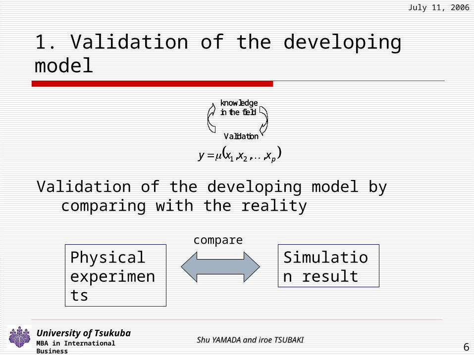
1. Validation of the developing model

Validation of the developing model by comparing with the reality

pxxxy ,,, 21

Validation

knowledge in the field

pxxxy ,,, 21

Validation


Validation


Physical experiments

Simulation result

compare

July 11, 2006



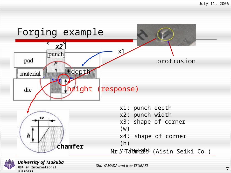
Forging example

protrusion

Mr. Taomoto (Aisin Seiki Co.)

height (response)

x1

chamfer

x1: punch depth x2: punch width x3: shape of corner (w)x4: shape of corner (h)y: height

depth

x2

July 11, 2006



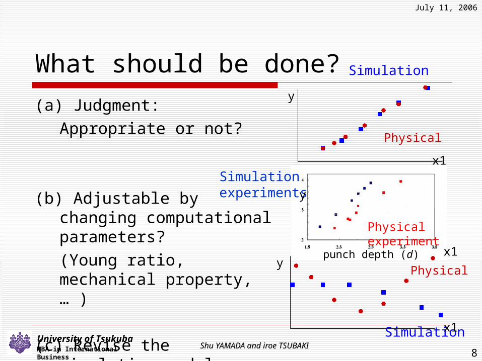
(a) Judgment:

Appropriate or not?

(b) Adjustable by changing computational parameters?

(Young ratio, mechanical property,… )

(c) Revise the simulation model

What should be done?

punch depth (d)

Simulation experiments

Physical experiment

Simulation

Physical

Physical

Simulation

y

y

y

x1

x1

x1

July 11, 2006



(a) Judgment: Appropriate or not?

Application of statistical tests

(b) Adjustable by changing computational parameters?

How to determine the level of the computational parameters systematically

(c) Revise the simulation model

Not a statistical problem

Simulation experiments

Physical experiment

July 11, 2006



Validation of the developing computer simulation model

punch depth (x1)

prot

rusi

on h

eigh

t

Simulation experimentsPhysical experiment

Adjusted simulation results

Find appropriate levels of computational parameters to fit the simulation results to physical experimental results

Computational parameters

Yong ratio, poison ratio, etc.

July 11, 2006



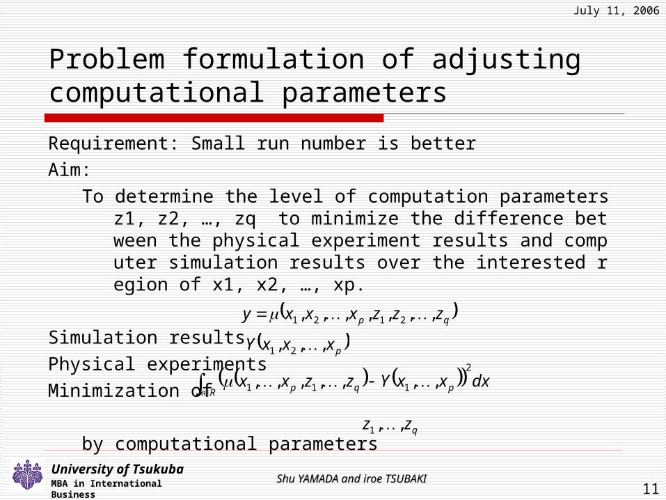
Problem formulation of adjusting computational parameters

Requirement: Small run number is better

Aim:

To determine the level of computation parameters z1, z2, …, zq to minimize the difference between the physical experiment results and computer simulation results over the interested region of x1, x2, …, xp.

Simulation results

Physical experiments

Minimization of

by computational parameters

dxxxYzzxxRx pqp

2

111 ,,,,,,,

qp zzzxxxy ,,,,,,, 2121

pxxxY ,,, 21

qzz ,,1

July 11, 2006



An approach by “easy to change” factor

Punch depth (x1) : Easy to change factor levels because it does not require remaking of mold. Physical experiments can be performed by using the mold by several levels.

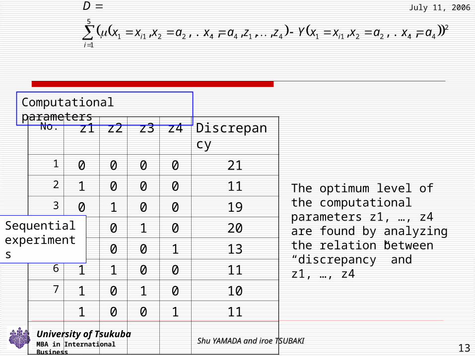
At each combination of computational parameters, the discrepancy between physical and experimental experiments are calculated by

5

1

244221141442211 ,...,,,,,,...,,

iii axaxxxYzzaxaxxx

D

July 11, 2006



No. z1 z2 z3 z4 Discrepancy

1 0 0 0 0 212 1 0 0 0 113 0 1 0 0 194 0 0 1 0 205 0 0 0 1 136 1 1 0 0 117 1 0 1 0 10

1 0 0 1 11

Computational parameters

5

1

244221141442211 ,...,,,,,,...,,

iii axaxxxYzzaxaxxx

D

Sequential experiments

The optimum level of the computational parameters z1, …, z4 are found by analyzing the relation between “discrepancy” and z1, …, z4

July 11, 2006



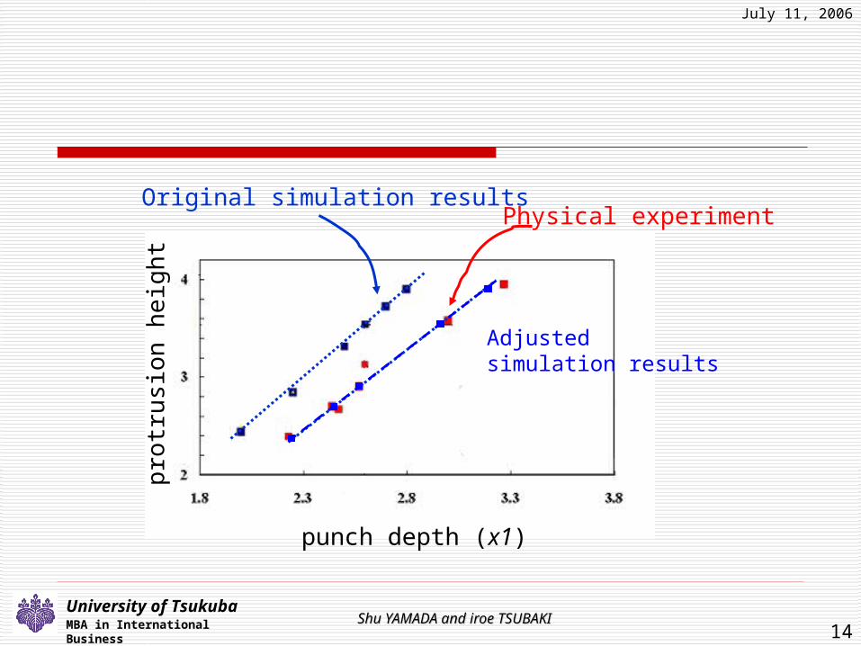
punch depth (x1)

prot

rusi

on h

eigh

t

Original simulation resultsPhysical experiment

Adjusted simulation results

July 11, 2006



Future problems at validation stage

(1) Statistical tests to judge the appropriateness of the simulation model

(2) Identification of the trend

(3) Design to examine the simulation model efficiently

July 11, 2006



2. Screening problemExample: cantilever

Ex. FEM measures the maximum stress

Factors x1, x2, …, xp

Theoretical equations (x1, x2, …, xp) are applied to calculate the respo

nse variables under given factor level

Design a beam in which one side is fixed to the wall

July 11, 2006



Design a beam (Iwata and Yamada (2004))

Stepping cantileverFactors

Hight 　 x1 ～ x15Levels No.1 30(mm)　　　　　 No.2 35(mm)

No.3 40(mm)Response

Maximum stressVariation of the maximum stress Weight of the beam

July 11, 2006



An application of three-level supersaturated design

Requirements

The relation between the responses and their factors are complicated

It takes several hours to calculate the response in a design

There are many factor effects

Linear effects 15

Interaction effects 105

Quadratic effects 15

Impossible to estimate all factor effects simultaneously.

July 11, 2006



Application of three-level supersaturated design

(Yamada and Lin (1999))

No. [1] [2] [3] [4] [5] [6] [7] [8] [9] [10] [11] [12] [13] [14] [15] [16] [17] [18] [19] [20] [21] [22] [23] [24] [25] [26] [27] [28] [29] [30]

1 1 1 1 1 1 1 1 1 1 1 1 1 1 1 1 1 1 1 1 1 1 1 1 1 1 1 1 1 1 1

2 1 1 2 2 2 3 1 3 2 3 3 2 1 2 3 1 2 3 1 3 2 1 2 2 2 3 1 3 2 3

3 1 1 3 3 3 3 3 2 1 2 3 1 2 3 1 3 2 3 3 2 1 1 3 3 3 3 3 2 1 2

4 1 2 1 2 3 3 2 1 3 3 1 3 2 3 2 1 3 1 3 3 3 2 1 2 3 3 2 1 3 3

5 1 2 2 3 1 2 3 1 2 3 2 1 3 3 3 2 1 3 2 1 3 2 2 3 1 2 3 1 2 3

6 1 2 3 1 2 2 2 3 1 2 2 3 1 1 3 3 3 2 3 1 2 2 3 1 2 2 2 3 1 2

7 1 3 1 3 2 2 1 2 3 1 3 3 3 2 2 3 1 2 2 3 1 3 1 3 2 2 1 2 3 1

8 1 3 2 1 3 1 3 3 3 2 1 2 3 2 1 2 3 2 1 2 3 3 2 1 3 1 3 3 3 2

9 1 3 3 2 1 1 2 2 2 1 2 2 2 1 2 2 2 1 2 2 2 3 3 2 1 1 2 2 2 1

10 2 1 1 1 1 1 1 1 1 1 1 1 1 1 1 1 1 1 1 1 1 2 2 2 2 2 2 2 2 2

11 2 1 2 2 2 3 1 3 2 3 3 2 1 2 3 1 2 3 1 3 2 2 3 3 3 1 2 1 3 1

12 2 1 3 3 3 3 3 2 1 2 3 1 2 3 1 3 2 3 3 2 1 2 1 1 1 1 1 3 2 3

13 2 2 1 2 3 3 2 1 3 3 1 3 2 3 2 1 3 1 3 3 3 3 2 3 1 1 3 2 1 1

14 2 2 2 3 1 2 3 1 2 3 2 1 3 3 3 2 1 3 2 1 3 3 3 1 2 3 1 2 3 1

15 2 2 3 1 2 2 2 3 1 2 2 3 1 1 3 3 3 2 3 1 2 3 1 2 3 3 3 1 2 3

16 2 3 1 3 2 2 1 2 3 1 3 3 3 2 2 3 1 2 2 3 1 1 2 1 3 3 2 3 1 2

17 2 3 2 1 3 1 3 3 3 2 1 2 3 2 1 2 3 2 1 2 3 1 3 2 1 2 1 1 1 3

18 2 3 3 2 1 1 2 2 2 1 2 2 2 1 2 2 2 1 2 2 2 1 1 3 2 2 3 3 3 2

19 3 1 1 1 1 1 1 1 1 1 1 1 1 1 1 1 1 1 1 1 1 3 3 3 3 3 3 3 3 3

20 3 1 2 2 2 3 1 3 2 3 3 2 1 2 3 1 2 3 1 3 2 3 1 1 1 2 3 2 1 2

21 3 1 3 3 3 3 3 2 1 2 3 1 2 3 1 3 2 3 3 2 1 3 2 2 2 2 2 1 3 1

22 3 2 1 2 3 3 2 1 3 3 1 3 2 3 2 1 3 1 3 3 3 1 3 1 2 2 1 3 2 2

23 3 2 2 3 1 2 3 1 2 3 2 1 3 3 3 2 1 3 2 1 3 1 1 2 3 1 2 3 1 2

24 3 2 3 1 2 2 2 3 1 2 2 3 1 1 3 3 3 2 3 1 2 1 2 3 1 1 1 2 3 1

25 3 3 1 3 2 2 1 2 3 1 3 3 3 2 2 3 1 2 2 3 1 2 3 2 1 1 3 1 2 3

26 3 3 2 1 3 1 3 3 3 2 1 2 3 2 1 2 3 2 1 2 3 2 1 3 2 3 2 2 2 1

27 3 3 3 2 1 1 2 2 2 1 2 2 2 1 2 2 2 1 2 2 2 2 2 1 3 3 1 1 1 3

July 11, 2006



Screening procedure

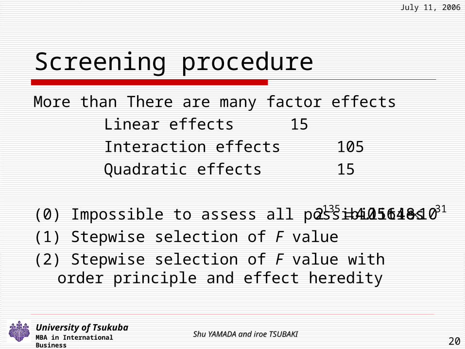
More than There are many factor effects

Linear effects 15

Interaction effects 105

Quadratic effects 15

(0) Impossible to assess all possibilities

(1) Stepwise selection of F value

(2) Stepwise selection of F value with order principle and effect heredity

31135 1005648.42

July 11, 2006



Analysis strategyOrder principle

Lower order terms are more important higher order terms

(Linear effect, interaction and quadratic,...)

Effect heredity

When two-factor interaction is detected,

(i) at least one factor effect of the two factors

(ii) both of the linear effects

should be included in the model. The strategy (ii) is implemented.

July 11, 2006



Procedure to ensure effect heredity and order principle (EO)

Step 1 Candidate set

Step 2

Quadratic term of the selected effect is added to the candidate set

Ex 1

Interaction term of the selected two factors is added

Ex 2

151,..., xx

2221151 ,,..., xxxxx

22151,..., xxx

July 11, 2006



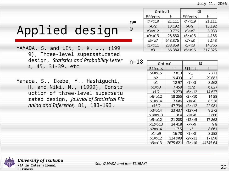
Applied designYAMADA, S. and LIN, D. K. J., (1999), Three-le

vel supersaturated design, Statistics and Probability Letters, 45, 31-39. etc

Yamada, S., Ikebe, Y., Hashiguchi, H. and Niki, N., (1999), Construction of three-level supersaturated design, Journal of Statistical Planning and Inference, 81, 183-193.

Eff ects F Eff ects Fx4×x10 21.111 x4×x10 21.111

x6 2̂ 13.192 x6 2̂ 13.192x3×x12 9.776 x3×x7 8.933x9×x13 28.830 x6×x13 4.185x5×x7 643.876 x7×x8 5.143x1×x11 288.850 x3×x8 14.766

x3 66.380 x6×x15 517.325

Ordi nal (i)

n=9

n=18Eff ects F Eff ects Fx6×x15 7.813 x１ 7.771

x2 9.433 x2 29.683x1 12.97 x1×x3 8.462

x1×x3 7.459 x1 2̂ 0.627x1 2̂ 9.279 x6×x12 14.027

x6×x12 18.255 x3×x10 14.88x1×x14 7.606 x1×x6 6.538x15 2̂ 47.734 x2×x12 22.981

x3×x14 23.437 x12×x4 9.372x10×x13 10.4 x2×x8 3.866x9×x12 21.208 x12×x5 17.868x12×x13 24.418 x7×x9 9.8x2×x14 17.5 x3 8.601x1×x9 16.78 x1×x8 8.158x1×x12 124.909 x2×x11 17.898x9×x13 2075.621 x7×x10 44345.04

Ordi nal (i)

July 11, 2006



What is a right choiceConsistency with the knowledge in the mechanical engineering

Physical property

1． The factors closing to the wall are important　　　　 such as x1,x2, x3

2. Sometimes, the edge side are important　　　　 such as x14, x15

3. Interaction can be considered at a connected two factors　　　　 such as x1×x2， x2×x3

x1 x4x3x2

x5 x15

July 11, 2006



EO select a reasonable selection in terms of the physical property of the cantilever

Effects F Effects F Effects Fx6×x15 7.813 x１ 7.771 x1 7.711

x2 9.433 x2 29.683 x2 29.683x1 12.97 x1×x3 8.462 x1 2̂ 6.066

x1×x3 7.459 x1 2̂ 0.627 x3 5.852x1 2̂ 9.279 x6×x12 14.027 x1×x3 10.466

x6×x12 18.255 x3×x10 14.88 x2 2̂ 28.566x1×x14 7.606 x1×x6 6.538 x×12 3.758x15 2̂ 47.734 x2×x12 22.981 x×7 5.631

x3×x14 23.437 x12×x4 9.372 x7×x12 9.498x10×x13 10.4 x2×x8 3.866 x3 2̂ 3.614x9×x12 21.208 x12×x5 17.868 x8 4.785x12×x13 24.418 x7×x9 9.8 x1×x2 8.77x2×x14 17.5 x3 8.601 x8×x12 5.445x1×x9 16.78 x1×x8 8.158 x4 2.8x1×x12 124.909 x2×x11 17.898 x4 2̂ 831.322x9×x13 2075.621 x7×x10 44345.04 x7 2̂ 156.486

n=18Ordinal EO

July 11, 2006



3. Approximation and optimizationExample: wire bonding in IC

Yamazaki, Masuda and Yoshino,(2005), Analysis of wire-loop resonance during al wire bonding, 11th Symposium on Microjoining in Electrics, February 3-4, 2005, Yokohama

Outline:Recent years AL wire bonding by microjoining is widely applied in many types of IC.

Finite Element Method obtained that it sometimes occurs resonance problem at the mircojoining.

July 11, 2006



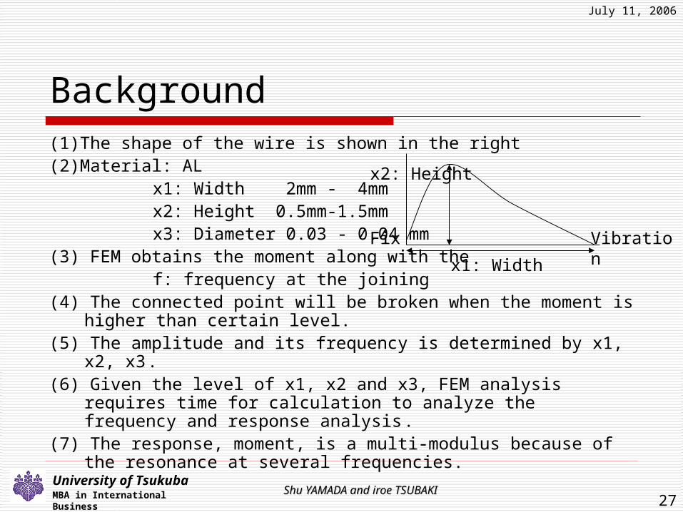
Background(1)The shape of the wire is shown in the right(2)Material: AL

x1: Width 2mm - 4mmx2: Height 0.5mm-1.5mm

x3: Diameter 0.03 - 0.04 mm (3) FEM obtains the moment along with the

f: frequency at the joining(4) The connected point will be broken when the moment is higher than

certain level.(5) The amplitude and its frequency is determined by x1, x2, x3．(6) Given the level of x1, x2 and x3, FEM analysis requires time for

calculation to analyze the frequency and response analysis．(7) The response, moment, is a multi-modulus because of the resonance at

several frequencies.

x1: Width

x2: Height

VibrationFix

July 11, 2006



Output of FEM software

x1: 3.14x2: 1.28x3: 0.03

x1: 3.00x2: 0.78x3: 0.03

FEMAP v8.2.1+ CAFEM v8.0

The peaks will be determined by x1: width, x2: height and x3: diameter

Complex function

July 11, 2006



Requirements(1)Outline of the factors in process

x1: Width Some restrictions because of the location with other parts

x2: Height controllable in the range (0.5-1.5mm)

x3: Diameter Specified in the priori process

f: Frequency Controllable by selecting the bonder

(2)The tentative levels of x1, x3 are determined in the priori process. Based on the tentative levels, optimum levels of x2 and f is explored. There is a need to consider the robustness against the difference of f from the specified value.

(3) It takes a long time to evaluate the frequency under a set of levels of x1, x2 and x3. Re-calculation is inefficient when the levels are slightly revised.

July 11, 2006



Strategy(1) The final goal is to find a good approximated function of M:

moment at the fixed point by x1: width, x2: height, x3: diameter and f: frequency such that

M=g(x1, x2, x3, f)

(2) In the future, various types of wires are applied in the IC design. Thus, the above approximation is helpful.

(3) To find a smooth function, 210-level design is utilized.

(4) Because of the complex relation, uniform design will be beneficial.

July 11, 2006



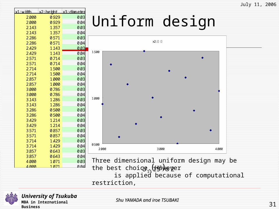
Uniform designx1: width x2: height x3: diameter

2.000 0.929 0.032.000 0.929 0.042.143 1.357 0.032.143 1.357 0.042.286 0.571 0.032.286 0.571 0.042.429 1.143 0.032.429 1.143 0.042.571 0.714 0.032.571 0.714 0.042.714 1.500 0.032.714 1.500 0.042.857 1.000 0.032.857 1.000 0.043.000 0.786 0.033.000 0.786 0.043.143 1.286 0.033.143 1.286 0.043.286 0.500 0.033.286 0.500 0.043.429 1.214 0.033.429 1.214 0.043.571 0.857 0.033.571 0.857 0.043.714 1.429 0.033.714 1.429 0.043.857 0.643 0.033.857 0.643 0.044.000 1.071 0.034.000 1.071 0.04

x2: 高さ

0.500

1.000

1.500

2.000 3.000 4.000

Three dimensional uniform design may be the best choice. However is applied because of computational restriction,

215215 U

July 11, 2006



http://www.math.hkbu.edu.hk/~ktfang/

July 11, 2006



x1: widthx2: heightx3: diameter2.000 0.929 0.032.000 0.929 0.042.143 1.357 0.032.143 1.357 0.042.286 0.571 0.032.286 0.571 0.042.429 1.143 0.032.429 1.143 0.042.571 0.714 0.032.571 0.714 0.042.714 1.500 0.032.714 1.500 0.042.857 1.000 0.032.857 1.000 0.043.000 0.786 0.033.000 0.786 0.043.143 1.286 0.033.143 1.286 0.043.286 0.500 0.033.286 0.500 0.043.429 1.214 0.033.429 1.214 0.043.571 0.857 0.033.571 0.857 0.043.714 1.429 0.033.714 1.429 0.043.857 0.643 0.033.857 0.643 0.044.000 1.071 0.034.000 1.071 0.04

frequency (210 levels)

x1: 3.14x2:1.28x3: 003

x1: 3.00x2: 0.78x3: 0.03

July 11, 2006



Approximation(1) It is beneficial to find levels of x1, x2, x3 and f with resonance

precisely rather than an well fitted model uniformly in the space of x1, x2, x3 and f.

(2) The main aim is to find levels x1, x2, x3 and f with resonance. The estimation of the moment is not the major aim.

(3) A RBF (radial basis function) like model is applied for the approximation.

＊ RBF is sometimes applied to describe the impulse response in neural network.

...2

1exp

2

1exp

2

1exp

2

3

33

2

2

22

2

1

1110

s

mfa

s

mfa

s

mfafbb

July 11, 2006



Model

5 10 15 20

020

4060

80

fr

y

5 10 15 20

020

4060

80

fr

pred

ict.c

...2

1exp

2

1exp

2

1exp

2

3

33

2

2

22

2

1

1110

s

mfa

s

mfa

s

mfafbb

f

fbb 10

1m 2m 3m

3s

2s1s

x1=3.00,

x2=0.78

X3=0.03

1a 2a

3a

July 11, 2006



x1: 3.14x2:1.28x3: 003

5 10 15 20

05

01

001

50

fr

y

5 10 15 20

05

01

001

50

fr

pre

dic

t.c

July 11, 2006



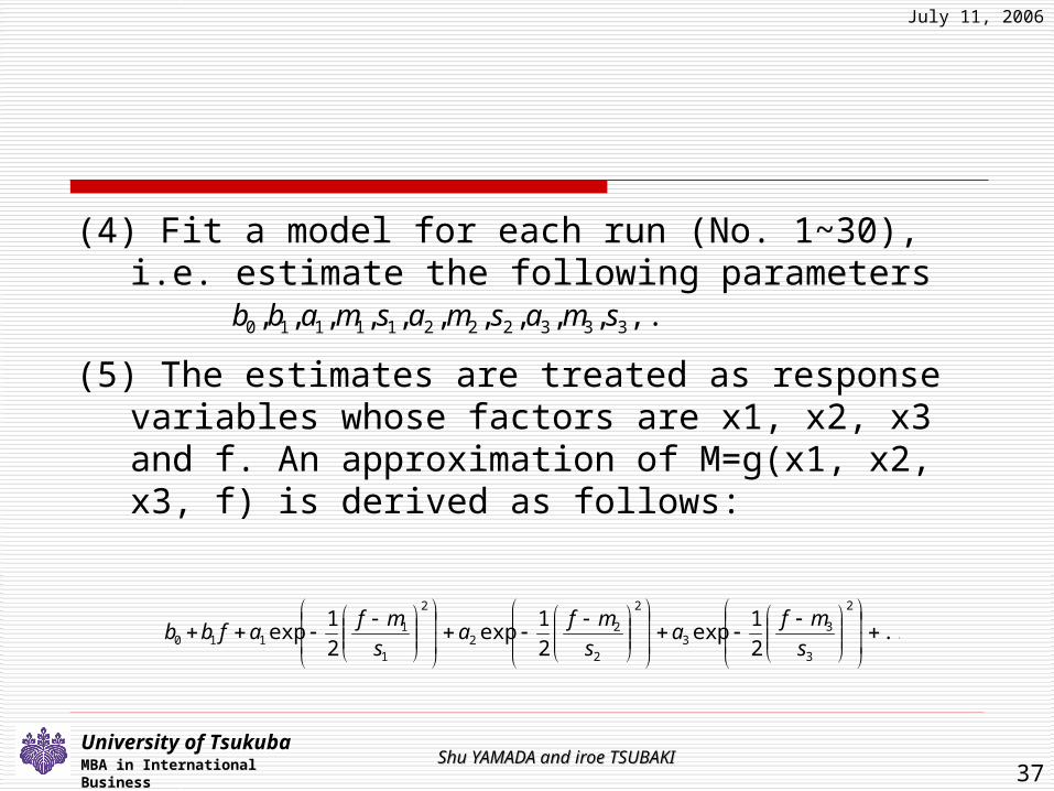
(4) Fit a model for each run (No. 1~30), i.e. estimate the following parameters

(5) The estimates are treated as response variables whose factors are x1, x2, x3 and f. An approximation of M=g(x1, x2, x3, f) is derived as follows:

,...,,,,,,,,,, 33322211110 smasmasmabb

...2

1exp

2

1exp

2

1exp

2

3

33

2

2

22

2

1

1110

s

mfa

s

mfa

s

mfafbb

July 11, 2006



(4) Fit a model for each run (No. 1~30), i.e. estimate the parameters

x1 x2 x3 b0 b1 a1 m1 s1 a2 m2 s2 a3 m3 s3 a4 m4 s4

2.000 0.929 0.03 17.670 0.623 282.100 6.343 0.205 198.000 13.930 0.391 1.000 1.000 1.000 1.000 1.000 1.000

2.000 0.929 0.04 52.260 -1.634 671.628 8.396 0.284

2.143 1.357 0.03 21.540 1.824 302.600 3.842 0.128 292.900 8.181 0.234 302.900 14.860 0.393

2.143 1.357 0.04 37.930 4.022 763.700 5.101 0.160 597.900 10.820 0.301 645.300 19.640 0.493

2.286 0.571 0.03 8.959 -0.090 40.913 7.422 0.194 15.110 18.500 0.363

2.286 0.571 0.04 31.385 -0.272 70.654 9.843 0.050

2.429 1.143 0.03 12.330 1.322 218.100 4.241 0.141 178.700 9.313 0.258 205.600 16.940 0.439

2.429 1.143 0.04 29.725 1.670 531.040 5.625 0.182 330.353 12.305 0.331

2.571 0.714 0.03 7.583 0.261 111.000 5.699 0.178 95.320 13.670 0.395

2.571 0.714 0.04 23.157 -0.468 227.231 7.523 0.239 155.645 18.090 0.570

2.714 1.500 0.03 18.510 1.341 191.600 2.842 0.104 207.000 6.130 0.174 220.800 11.150 0.301 204.000 17.460 0.422

2.714 1.500 0.04 33.480 2.874 525.700 3.781 0.119 417.200 8.120 0.226 473.400 14.780 0.391

2.857 1.000 0.03 10.875 -0.063 113.908 3.951 0.132 80.169 9.102 0.258 73.502 16.331 0.454

2.857 1.000 0.04 17.040 0.419 272.300 5.232 0.174 116.000 12.040 0.299

3.000 0.786 0.03 0.586 0.586 44.980 4.216 0.157 28.530 10.330 0.245 59.780 18.110 0.500

3.000 0.786 0.04 17.831 -0.626 84.585 5.573 0.150 8.239 13.995 0.353

3.143 1.286 0.03 16.776 -0.217 157.526 2.893 0.074 112.730 6.481 0.180 124.995 11.758 0.347 46.940 17.826 0.386

3.143 1.286 0.04 25.530 0.505 316.400 3.829 0.125 206.000 8.584 0.234 248.100 15.560 0.433

3.286 0.500 0.03 -11.743 2.958 62.348 4.222 0.178 34.831 11.114 0.154 288.200 17.869 0.495

3.286 0.500 0.04 22.721 0.754 216.967 5.538 0.161 118.535 14.752 0.309

3.429 1.214 0.03 9.249 0.031 109.600 2.710 0.076 75.270 6.254 0.180 72.680 11.250 0.315 7.658 17.250 0.207

3.429 1.214 0.04 21.301 -0.345 252.741 3.604 0.099 127.970 8.289 0.227 117.079 14.870 0.407

3.571 0.857 0.03 1.061 29.487 3.089 0.074 21.239 7.688 0.138 59.114 13.309 0.309 140.716 20.338 0.485

3.571 0.857 0.04 255.737 17.6878 0.8923

3.714 1.429 0.03 11.540 -0.095 98.762 2.186 0.070 87.177 4.933 0.142 92.258 8.929 0.261 30.218 13.523 0.265

3.714 1.429 0.04 20.490 0.322 281.000 2.894 0.076 161.700 6.544 0.182 179.700 11.830 0.329 30.060 18.210 0.313

3.857 0.643 0.03 -6.811 2.330 30.954 3.022 0.134 20.396 7.821 0.112 164.662 12.8338 0.3548 105.416 20.275 0.389

3.857 0.643 0.04 -31.606 7.409 108.136 3.992 0.208 32.853 10.362 0.092 597.156 16.780 0.455

4.000 1.071 0.03 0.000 0.871 31.305 2.348 0.111 31.679 5.714 0.148 6.000 10.000 0.050 71.379 15.301 0.400

4.000 1.071 0.04 0.000 19.129 75.876 3.108 0.072 35.098 7.585 0.115 100.634 13.345 0.362 401.240 20.136 0.587

July 11, 2006



(5) The estimates are treated as response variables whose factors are x1, x2, x3 and f.

b0 b1 a1 m1 s1 a2 m2 s2 a3 m3 s3

Constant -96.1 53.0 -743.0 14.6 0.1 -346.0 35.7 0.2 -1779.1 37.1 -2.0

x1 15.6 -32.0 12.5 -6.4 0.0 -68.9 -12.6 -0.2 -98.9 -11.4 0.8

x2 -37.3 16.6 252.9 -10.1 0.1 -131.4 -27.8 -0.5 -400.3 -21.7 0.7

z3 5640.0 -1125.3 32652.3 391.5 1.9 30519.3 746.6 44.5 126459.5 909.8 53.4

x1*x2 19.1 -5.5 -261.3 2.8 -0.1 -187.0 6.3 0.3 -89.9 6.1

x1*x3 -1465.8 433.7 -12456.0 -59.3 -10519.6 -88.2 -7.9 -17220.4 -98.4

x2*x3 22767.2 -86.5 10586.4 -196.6 -12.5 -42641.2 -175.3 -30.5

x1 2̂ 4.1 87.0 0.6 81.2 0.9 98.2 0.4 -0.2

x2 2̂ 0.8 269.9 3.4 934.8 -0.9

...2

1exp

2

1exp

2

1exp

2

3

33

2

2

22

2

1

1110

s

mfa

s

mfa

s

mfafbb

213211

22

213231213211

213231213211

2131213211

31213210

1.09.10.10.0-0 0.1

0.8 0.686.5-59.3-2.8391.510.1-6.4-14.6

87.022767.212456.0-261.3-32652.3252.912.5-743.0a

4.1433.75.5-1125.3-16.632.0-53.0

1465.8-19.15640.037.3-6.151.96

xxxxxs

xxxxxxxxxxxm

xxxxxxxxxx

xxxxxxxxb

xxxxxxxb

July 11, 2006



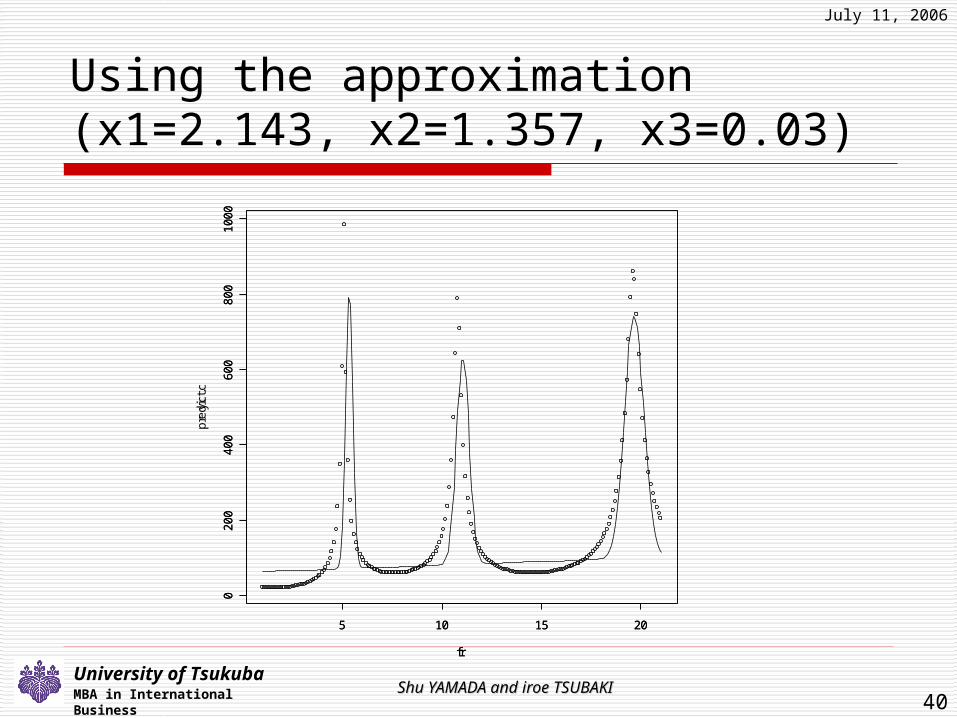
Using the approximation(x1=2.143, x2=1.357, x3=0.03)

5 10 15 20

02

00

40

06

00

80

01

00

0

fr

y

5 10 15 20

02

00

40

06

00

80

01

00

0

fr

pre

dic

t.c

July 11, 2006



(x1=3.000, x2=0.786, x3=0.03)

5 10 15 20

02

040

60

80

fr

y

5 10 15 20

02

040

60

80

fr

pre

dic

t.c

July 11, 2006



Comments(1) The essence of the case study is exploring an approximation of

multi-modulus function by uniform design and RBF.

(2) Fitting by RBF brings a good fitting. It is suggested that RBF is beneficial to fit response to frequency.

(3) It is concerned the over fitting in the case study. The fitness should be validated.

(4) The parameters a1, m1, a2, m2,… are estimated precisely, for example the adjusted R^2 is more than 90%. On the other hand, there is a need to estimate s1, s2, … more precisely.

July 11, 2006



5

10

15

20 0.5

0.6

0.7

0.8

0.9

1

0

5

10

15

5

10

15

205 10 15 20

0.5

0.6

0.7

0.8

0.9

1

Application of the approximation

x1: width 3mm, x3 diameter 0.3

ｘ 2 height

ｘ 2 height

frequency

f

Good choice

July 11, 2006



4. Grammar of DOE in computer simulation study

1. Interpreting requirements

2. Developing a simulator

3. Applying the simulator

pxxxy ,,, 21

3333

2111311332110

31

ˆˆˆˆˆˆ

,ˆ

xxxxxx

xxy

Optimization from various viewpoints

Output

Input

yDefine

pxxx ,,, 21

Validation


Validation: Comparison of simulation results to reality

Application of DOE depending on the situation

pxxxxx ,,,,, 4321

Stage Design AnalysisFractionalfactorial designSupersaturateddesignCentralcomposite

Second ordermodel

Spece fillingdesign

Various models

Screening

Approximation

Stepwise selectionby F statisitc

university of tsukuba mba in international business july 11, 2006 1 application of design of...

Documents