User Note for Relativistic EOS Table

(EOS1: 1998-version, with only nucleons)

H. Shena1, H. Tokib2, K. Oyamatsuc3, and K. Sumiyoshid4

aDepartment of Physics, Nankai University, Tianjin 300071, China

bResearch Center for Nuclear Physics (RCNP), Osaka University, Ibaraki, Osaka 567-0047,

Japan

cDepartment of Media Theories and Production, Aichi Shukutoku University, Nagakute-cho,

Aichi 480-1197, Japan

dNumazu College of Technology, Ooka 3600, Numazu, Shizuoka 410-8501, Japan

Abstract

This is a detailed note for users of the relativistic equation of state (EOS) of nuclear

matter.

Contents

• 1 Introduction

• 2 Relativistic mean-field theory

• 3 Ideal-gas approximation

• 4 Thomas-Fermi approximation

• 5 Calculation procedure in detail

• 6 Resulting EOS table

• 7 Suggestions for using the EOS table

1e-mail: shennankai@gmail.com2e-mail: toki@rcnp.osaka-u.ac.jp3e-mail: oyak@asu.aasa.ac.jp4e-mail: sumi@numazu-ct.ac.jp

1

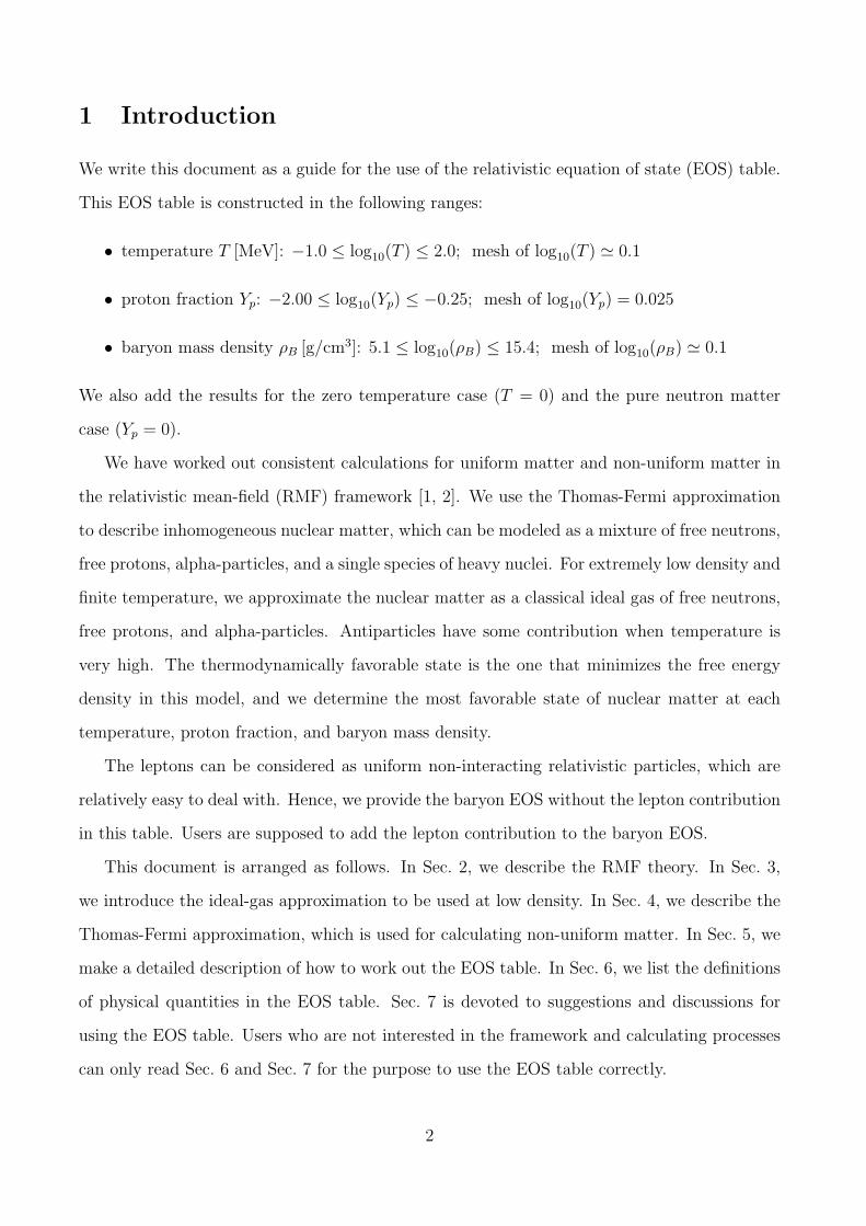
1 Introduction

We write this document as a guide for the use of the relativistic equation of state (EOS) table.

This EOS table is constructed in the following ranges:

• temperature T [MeV]: −1.0 ≤ log10(T ) ≤ 2.0; mesh of log10(T ) ' 0.1

• proton fraction Yp: −2.00 ≤ log10(Yp) ≤ −0.25; mesh of log10(Yp) = 0.025

• baryon mass density ρB [g/cm3]: 5.1 ≤ log10(ρB) ≤ 15.4; mesh of log10(ρB) ' 0.1

We also add the results for the zero temperature case (T = 0) and the pure neutron matter

case (Yp = 0).

We have worked out consistent calculations for uniform matter and non-uniform matter in

the relativistic mean-field (RMF) framework [1, 2]. We use the Thomas-Fermi approximation

to describe inhomogeneous nuclear matter, which can be modeled as a mixture of free neutrons,

free protons, alpha-particles, and a single species of heavy nuclei. For extremely low density and

finite temperature, we approximate the nuclear matter as a classical ideal gas of free neutrons,

free protons, and alpha-particles. Antiparticles have some contribution when temperature is

very high. The thermodynamically favorable state is the one that minimizes the free energy

density in this model, and we determine the most favorable state of nuclear matter at each

temperature, proton fraction, and baryon mass density.

The leptons can be considered as uniform non-interacting relativistic particles, which are

relatively easy to deal with. Hence, we provide the baryon EOS without the lepton contribution

in this table. Users are supposed to add the lepton contribution to the baryon EOS.

This document is arranged as follows. In Sec. 2, we describe the RMF theory. In Sec. 3,

we introduce the ideal-gas approximation to be used at low density. In Sec. 4, we describe the

Thomas-Fermi approximation, which is used for calculating non-uniform matter. In Sec. 5, we

make a detailed description of how to work out the EOS table. In Sec. 6, we list the definitions

of physical quantities in the EOS table. Sec. 7 is devoted to suggestions and discussions for

using the EOS table. Users who are not interested in the framework and calculating processes

can only read Sec. 6 and Sec. 7 for the purpose to use the EOS table correctly.

2

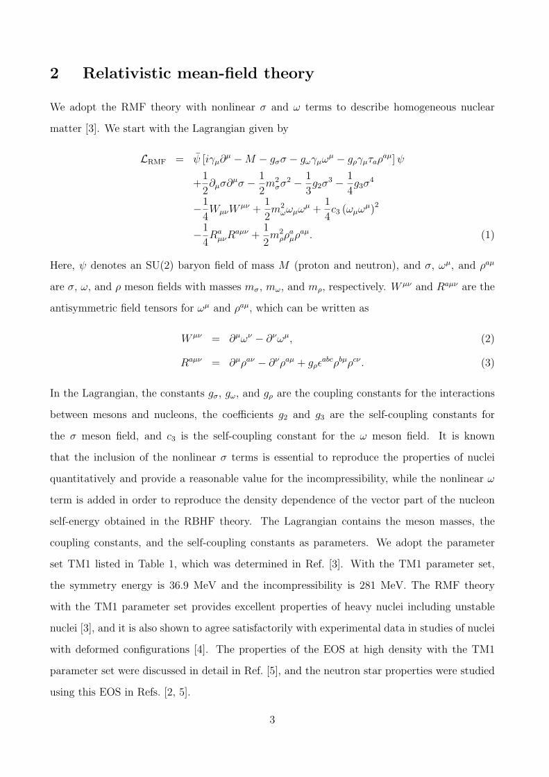
2 Relativistic mean-field theory

We adopt the RMF theory with nonlinear σ and ω terms to describe homogeneous nuclear

matter [3]. We start with the Lagrangian given by

LRMF = ψ [iγµ∂µ −M − gσσ − gωγµω

µ − gργµτaρaµ] ψ

+1

2∂µσ∂µσ − 1

2m2

σσ2 − 1

3g2σ

3 − 1

4g3σ

4

−1

4WµνW

µν +1

2m2

ωωµωµ +

1

4c3 (ωµω

µ)2

−1

4Ra

µνRaµν +

1

2m2

ρρaµρ

aµ. (1)

Here, ψ denotes an SU(2) baryon field of mass M (proton and neutron), and σ, ωµ, and ρaµ

are σ, ω, and ρ meson fields with masses mσ, mω, and mρ, respectively. W µν and Raµν are the

antisymmetric field tensors for ωµ and ρaµ, which can be written as

W µν = ∂µων − ∂νωµ, (2)

Raµν = ∂µρaν − ∂νρaµ + gρεabcρbµρcν . (3)

In the Lagrangian, the constants gσ, gω, and gρ are the coupling constants for the interactions

between mesons and nucleons, the coefficients g2 and g3 are the self-coupling constants for

the σ meson field, and c3 is the self-coupling constant for the ω meson field. It is known

that the inclusion of the nonlinear σ terms is essential to reproduce the properties of nuclei

quantitatively and provide a reasonable value for the incompressibility, while the nonlinear ω

term is added in order to reproduce the density dependence of the vector part of the nucleon

self-energy obtained in the RBHF theory. The Lagrangian contains the meson masses, the

coupling constants, and the self-coupling constants as parameters. We adopt the parameter

set TM1 listed in Table 1, which was determined in Ref. [3]. With the TM1 parameter set,

the symmetry energy is 36.9 MeV and the incompressibility is 281 MeV. The RMF theory

with the TM1 parameter set provides excellent properties of heavy nuclei including unstable

nuclei [3], and it is also shown to agree satisfactorily with experimental data in studies of nuclei

with deformed configurations [4]. The properties of the EOS at high density with the TM1

parameter set were discussed in detail in Ref. [5], and the neutron star properties were studied

using this EOS in Refs. [2, 5].

3

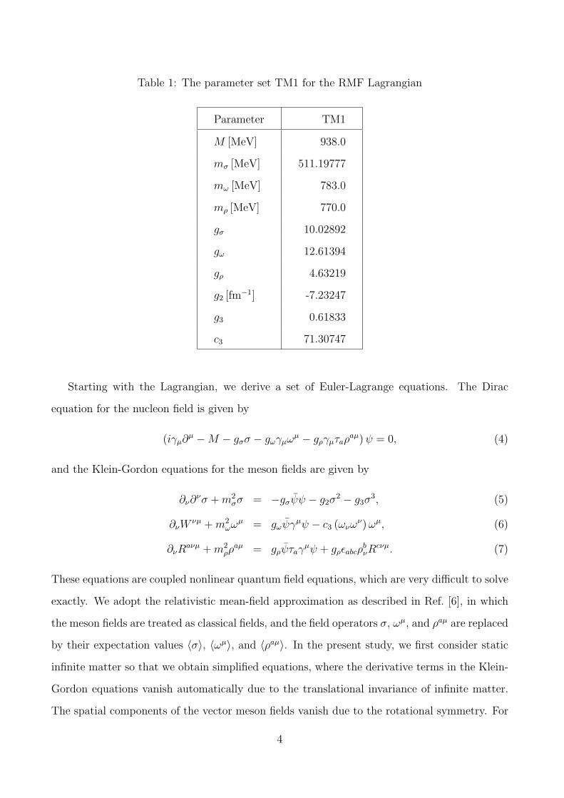
Table 1: The parameter set TM1 for the RMF Lagrangian

Parameter TM1

M [MeV] 938.0

mσ [MeV] 511.19777

mω [MeV] 783.0

mρ [MeV] 770.0

gσ 10.02892

gω 12.61394

gρ 4.63219

g2 [fm−1] -7.23247

g3 0.61833

c3 71.30747

Starting with the Lagrangian, we derive a set of Euler-Lagrange equations. The Dirac

equation for the nucleon field is given by

(iγµ∂µ −M − gσσ − gωγµω

µ − gργµτaρaµ) ψ = 0, (4)

and the Klein-Gordon equations for the meson fields are given by

∂ν∂νσ + m2

σσ = −gσψψ − g2σ2 − g3σ

3, (5)

∂νWνµ + m2

ωωµ = gωψγµψ − c3 (ωνων) ωµ, (6)

∂νRaνµ + m2

ρρaµ = gρψτaγ

µψ + gρεabcρbνR

cνµ. (7)

These equations are coupled nonlinear quantum field equations, which are very difficult to solve

exactly. We adopt the relativistic mean-field approximation as described in Ref. [6], in which

the meson fields are treated as classical fields, and the field operators σ, ωµ, and ρaµ are replaced

by their expectation values 〈σ〉, 〈ωµ〉, and 〈ρaµ〉. In the present study, we first consider static

infinite matter so that we obtain simplified equations, where the derivative terms in the Klein-

Gordon equations vanish automatically due to the translational invariance of infinite matter.

The spatial components of the vector meson fields vanish due to the rotational symmetry. For

4

the isovector-vector meson field ρaµ, only the third isospin component has a non-vanishing value

because of the charge conservation. Hence, the equations for the meson fields are reduced to

σ0 ≡ 〈σ〉 = − gσ

m2σ

〈ψψ〉 − 1

m2σ

(g2σ

20 + g3σ

30

), (8)

ω0 ≡ 〈ω0〉 =gω

m2ω

〈ψγ0ψ〉 − 1

m2ω

c3ω30, (9)

ρ0 ≡ 〈ρ30〉 =gρ

m2ρ

〈ψτ3γ0ψ〉. (10)

The Dirac equation then becomes

(−iαk∇k + βM∗ + gωω0 + gρτ3ρ0

)ψis = εisψis, (11)

where the index i denotes the isospin degree of freedom (proton and neutron), s denotes the

index of eigenstates of nucleon, M∗ ≡ M + gσσ0 is the effective nucleon mass, and εis is the

single-particle energy.

Nucleons occupy single-particle orbits with the occupation probability fis. At zero tem-

perature, fis = 1 under the Fermi surface, while fis = 0 above the Fermi surface. For finite

temperature, the occupation probability is given by the Fermi-Dirac distribution,

fis =1

1 + exp [(εis − µi) /T ]=

1

1 + exp[(√

k2 + M∗2 − νi

)/T

] , (12)

fis =1

1 + exp [(−εis + µi) /T ]=

1

1 + exp[(√

k2 + M∗2 + νi

)/T

] . (13)

Here the indices i and i denote nucleons and antinucleons, and εis and εis are the single-particle

energy of nucleons and antinucleons, respectively. The relation between the chemical potential

µi and the kinetic part of the chemical potential νi is give by

µi = νi + gωω0 + gρτ3ρ0. (14)

The chemical potential µi is related to the number density of nucleon ni as

ni =γ

2π2

∫ ∞

0dk k2 (fik − fik) , (15)

where γ is the degeneracy factor for the spin degree of freedom (γ = 2). The quantum number

s is replaced by the momentum k when we do the integration in the momentum space instead

5

of summing over the eigenstates. The equations of the meson fields can be written as

σ0 = − gσ

m2σ

∑

i

γ

2π2

∫ ∞

0dk k2 M∗

√k2 + M∗2

(fik + fik)−1

m2σ

(g2σ

20 + g3σ

30

), (16)

ω0 =gω

m2ω

(np + nn)− c3

m2ω

ω30, (17)

ρ0 =gρ

m2ρ

(np − nn) . (18)

Here, np and nn are the proton and neutron number densities as defined in Eq. (15), and we

denote nB = np + nn as the baryon number density. We solve these equations self-consistently.

The thermodynamical quantities are described in Ref. [6], and we simply write the expressions

here. The energy density of nuclear matter is given by

ε =∑

i

γ

2π2

∫ ∞

0dk k2

√k2 + M∗2 (fik + fik) +

1

2m2

σσ20 +

1

3g2σ

30 +

1

4g3σ

40

+gωω0 (np + nn)− 1

2m2

ωω20 −

1

4c3ω

40

+gρρ0 (np − nn)− 1

2m2

ρρ20, (19)

the pressure of nuclear matter is given by

p =∑

i

γ

6π2

∫ ∞

0dk k2 k2

√k2 + M∗2

(fik + fik)−1

2m2

σσ20 −

1

3g2σ

30 −

1

4g3σ

40

+1

2m2

ωω20 +

1

4c3ω

40 +

1

2m2

ρρ20, (20)

and the entropy density is calculated by

s =∑

i

γ

2π2

∫ ∞

0dk k2 [−fik ln fik − (1− fik) ln (1− fik)

−fik ln fik − (1− fik) ln (1− fik)] . (21)

3 Ideal-gas approximation

The interaction between nucleons is negligible at low density, so that we can treat nucleons

as non-interacting Boltzmann particles at low density. We use the ideal-gas approximation

to describe the mixed gas of neutrons, protons, and alpha-particles at low density and finite

temperature. We note that the connection between the RMF results and the ideal-gas approx-

imation is smooth.

6

For Boltzmann particles with spin 1/2, mass M , and number density ni (i is n or p), we

start with the partition function given by

Zi =[(nQ)ni/2/(ni/2)!

]2, (22)

where we have used the abbreviation nQ =(

MT2π

)3/2. The factor (ni/2)! comes from avoiding the

double counting for ni/2 indistinguishable particles of spin up or spin down. We can calculate

the free energy density from the partition function as

fi = −T ln Zi = −T ni [ln(2nQ/ni) + 1] . (23)

The entropy density is given by

si = −(

∂fi

∂T

)

ni

= ni

[ln(2nQ/ni) +

5

2

], (24)

the internal energy density can be written as

εi = fi + Tsi =3

2T ni, (25)

the chemical potential is obtained through the relation

µi =

(∂fi

∂ni

)

T

= −T ln(2nQ/ni), (26)

and the pressure is given by

pi =

[n2

i

∂ (fi/ni)

∂ni

]

T

= T ni. (27)

The partition function of alpha-particles can be written as

Zα = [8nQ exp (Bα/T )]nα /nα!, (28)

where nα is the alpha-particle number density, and Bα = 28.3 MeV is the binding energy of

an alpha-particle taken from Ref. [7]. The thermodynamical quantities of alpha-particles are

given by

fα = −T nα [ln(8nQ/nα) + 1]− nαBα, (29)

sα = nα

[ln(8nQ/nα) +

5

2

], (30)

εα =3

2T nα − nαBα, (31)

µα = −T ln(8nQ/nα)−Bα, (32)

pα = T nα. (33)

7

For a mixed gas with the neutron number density nn, the proton number density np, and

the alpha-particle number density nα, the free energy density is given by

f = fn + fp + fα. (34)

We have to take into account the volume of the alpha-particle, otherwise the alpha-particle

fraction would be some big number at high densities, where the alpha-particles should actually

disappear. When we take into account the volume excluded by the alpha-particles, the free

energy densities in Eq. (34) are given by

fn = −(1− u) T nn [ln(2nQ/nn) + 1] , (35)

fp = −(1− u) T np [ln(2nQ/np) + 1] , (36)

fα = −(1− u) {T nα [ln(8nQ/nα) + 1]− nαBα} , (37)

where u = nαvα is the fraction of space occupied by alpha-particles with the effective volume of

an alpha-particle vα = 24 fm−3 taken from Ref. [7]. We denote the effective number densities of

neutrons, protons, and alpha-particles as nn = nn/(1−u), np = np/(1−u), and nα = nα/(1−u).

The inclusion of the volume excluded by the alpha-particles has negligible effect in the low

density region, while it is necessary for the calculation at high density. Actually, we just use

Eqs. (35) and (36) for the case of nn+np < 10−5 fm−3, while the RMF theory is used to describe

nucleons when nn + np > 10−5 fm−3. For alpha-particles, we use Eq. (37) to calculate the free

energy in the whole density range. It is considered as a reasonable approximation because the

number density of alpha-particles is not so large even though the total baryon density is high,

and the alpha-particle fraction tends to vanish in the high density limit.

For very high temperature, we need to consider the contribution from antiparticles. The

alpha-particle fraction is very small at high temperature, so we can treat the matter as uniform

matter of nucleons and antinucleons. We have included the freedom of antiparticles in the RMF

theory, but the RMF code meets some difficulty at extremely low density, so we need to take

some approximation in order to describe the range of low density and high temperature. We

take the nonrelativistic approximation of the RMF theory at low density, where the effective

nucleon mass M∗ ≈ M , < mesons >≈ 0, and√

k2 + M∗2 ≈ M + k2

2M. Then the occupation

8

probability of the Fermi-Dirac distribution becomes

fis = ACi exp(−k2/2MT

), (38)

fis =A

Ci

exp(−k2/2MT

), (39)

where A = exp (−M/T ), and Ci = exp (µi/T ) with µi being the chemical potential of protons

(i = p) or neutrons (i = n), which is related to the number density ni as

ni = 2A(Ci − 1

Ci

) (MT

2π

)3/2

. (40)

The thermodynamical quantities can be approximated as

εi = 2A(Ci +

1

Ci

) (MT

2π

)3/2 (3

2T

), (41)

pi = 2A(Ci +

1

Ci

) (MT

2π

)3/2

T, (42)

si = 2A[5

2

(Ci +

1

Ci

)− Ci ln (ACi)− 1

Ci

ln(

A

Ci

)] (MT

2π

)3/2

. (43)

The contribution from antiparticles is negligible when Ci À 1/Ci, where the above expressions

agree with the ideal-gas approximation.

4 Thomas-Fermi approximation

In the range, T < 15 MeV and ρB < 1014.2 g/cm3, where heavy nuclei may be formed in order

to lower the free energy, we perform the Thomas-Fermi calculation based on the work done

by Oyamatsu [8]. In this case, the non-uniform matter can be modeled as a mixture of free

neutrons, free protons, alpha-particles, and a single species of heavy nuclei, while the leptons

can be treated as uniform non-interacting particles separately. For the system with fixed proton

fraction, the leptons play no role in the minimization of the free energy. Hence we mainly pay

attention to baryon contribution in this calculation. Hereafter, we will not mention the leptons

frequently, while we should keep in mind that there exists a uniform lepton gas everywhere.

We assume that each heavy spherical nucleus is located in the center of a charge-neutral

cell consisting of a vapor of neutrons, protons, and alpha-particles. The nuclei form a body-

centered-cubic (BCC) lattice to minimize the Coulomb lattice energy. It is useful to introduce

9

the Wigner-Seitz cell to simplify the energy of a unit cell. The Wigner-Seitz cell is a sphere

whose volume is the same as the unit cell in the BCC lattice. We define the lattice constant a

as the cube root of the cell volume. Then, we have

Vcell = a3 = NB/nB, (44)

where NB and nB are the baryon number per cell and the average baryon number density,

respectively. We define the baryon mass density as ρB = munB with mu being the atomic mass

unit. We calculate the Coulomb energy using this Wigner-Seitz approximation and add an

energy correction for the BCC lattice [8]. This energy correction is negligible unless the nuclear

size is comparable to the cell size.

We assume the nucleon distribution function ni(r) (i = n for neutron, i = p for proton) in

the Wigner-Seitz cell as

ni (r) =

(nin

i − nouti

) [1−

(r

Ri

)ti]3

+ nouti , 0 ≤ r ≤ Ri,

nouti , Ri ≤ r ≤ Rcell,

(45)

where r represents the distance from the center of the nucleus and Rcell is the radius of the

Wigner-Seitz cell defined by the relation

Vcell ≡ 4π

3R3

cell. (46)

The density parameters nini and nout

i are the densities at r = 0 and r ≥ Ri, respectively. The

parameters Ri and ti determine the boundary and the relative surface thickness of the heavy

nucleus.

For the distribution function of alpha-particle nα(r), which should decrease as r approaches

the center of the heavy nucleus, we assume

nα (r) =

−noutα

[1−

(r

Rp

)tp]3

+ noutα , 0 ≤ r ≤ Rp,

noutα , Rp ≤ r ≤ Rcell,

(47)

which could give nα(r = 0) = 0 and nα(r > Rp) = noutα . Here we use the same parameters Rp

and tp for both proton and alpha-particle distribution functions in order to avoid the presence

of too many parameters in the minimization procedure. The parameters Rn and tn may be

somewhat different from Rp and tp due to the additional neutrons forming a neutron skin in the

10

surface region. For a system with fixed temperature T , proton fraction Yp, and baryon mass

density ρB, there are eight independent parameters among the ten variables, a, ninn , nout

n , Rn,

tn, ninp , nout

p , Rp, tp, and noutα . The thermodynamically favorable state is the one that minimizes

the free energy density with respect to these eight independent parameters.

In this model the free energy density contributed from baryons is given by

f = Fcell / a3 = ( Ecell − T Scell ) / a3, (48)

where the free energy per cell Fcell can be written as

Fcell = (Ebulk + Es + EC)− TScell = Fbulk + Es + EC . (49)

The bulk energy Ebulk, entropy Scell, and bulk free energy Fbulk are calculated by

Ebulk =∫

cellε ( nn (r) , np (r) , nα (r) ) d3r, (50)

Scell =∫

cells ( nn (r) , np (r) , nα (r) ) d3r, (51)

Fbulk =∫

cellf ( nn (r) , np (r) , nα (r) ) d3r. (52)

Here ε ( nn (r) , np (r) , nα (r) ), s ( nn (r) , np (r) , nα (r) ), and f ( nn (r) , np (r) , nα (r) ) are the

local energy density, entropy density, and free energy density at the radius r, where the system

can be considered as a mixed uniform matter of neutrons, protons, and alpha-particles. Note

that these local densities at each radius are calculated by treating neutrons and protons in the

RMF theory as described in Sec. 2 for the case of nn(r) + np(r) > 10−5 fm−3, while we can use

the method described in Sec. 3 for low density case of nn(r) + np(r) < 10−5 fm−3.

As for the surface energy term Es due to the inhomogeneity of the nucleon distribution, we

take the simple form

Es =∫

cellF0 | ∇ ( nn (r) + np (r) ) |2 d3r. (53)

The parameter F0 = 70 MeV · fm5 is determined by performing the Thomas-Fermi calculations

for finite nuclei so as to reproduce the gross properties of the nuclear mass, charge radii, and

the beta stability line as described in the Appendix of Ref. [8].

The Coulomb energy per cell EC is calculated using the Wigner-Seitz approximation with

an added correction term for the BCC lattice [8]

EC =1

2

∫

celle [np (r) + 2nα (r)− ne] φ(r)d3r + 4EC , (54)

11

where φ(r) represents the electrostatic potential calculated in the Wigner-Seitz approximation,

ne is the electron number density of a uniform electron gas (ne = Yp nB), and 4EC is the

correction term for the BCC lattice, which can be approximated as

4EC = CBCC(Znone)

2

a. (55)

Here a is the lattice constant as defined in Eq. (44), the coefficient CBCC = 0.006562 is taken

from Ref. [8], and Znon is the non-uniform part of the charge number per cell given by

Znon =∫ Rp

0(nin

p − noutp − 2nout

α )

1−

(r

Rp

)tp

3

4πr2dr. (56)

Because of the long-range nature of the Coulomb interaction, the Coulomb energy will depend

on the lattice type. This dependence was discussed in more detail in Ref. [8]. The system

prefers the BCC lattice because the BCC lattice gives the lowest Coulomb energy.

5 Calculation procedure in detail

We calculate the EOS table in the range mentioned in Sec. 1. For each T , Yp, and ρB, we

perform the minimization of the free energy for non-uniform matter using the Thomas-Fermi

method described in Sec. 4. We also do the minimization for uniform matter with respect

to converting two protons and two neutrons into an alpha-particle, in which there is only one

independent parameter. Here, the phase of heavy nuclei formed together with free nucleons and

alpha-particles is referred to as non-uniform matter, while the phase of nucleons mixed with

alpha-particles without heavy nuclei is referred to as uniform matter. By comparing the free

energy of non-uniform matter with that of uniform matter, we determine the most favorable

state of nuclear matter at this T , Yp, and ρB. The density of the phase transition between

uniform matter and non-uniform matter depends on both T and Yp. The non-uniform matter

phase can exist only in the low temperature range (T < 15 MeV).

We construct the EOS table in three dimensions (T , Yp, and ρB). We first fix T , and then

fix Yp and ρB. We finish the following steps in order to work out an EOS table with fixed T

where the non-uniform matter phase exists.

• 1 calculate input table in the RMF theory for the use of minimization

12

• 2 do minimization for uniform matter at low density

• 3 do minimization for non-uniform matter at medium density

• 4 calculate the RMF result for uniform matter without alpha-particles at high density

• 5 determine the phase transition and connect the free energy

• 6 calculate the pressure and chemical potentials from the free energy

• 7 construct the finial EOS table at this T

Now, we explain each step in more detail.

• 1 The calculation of the minimization procedure needs the free energy per baryon as a

function of nn and np as input table, and this input table should be big enough in order to get

good numerical accuracy in doing linear approximation. We calculate this input table in the

RMF theory which can describe the homogeneous matter of protons and neutrons. This input

table covers the following range

Yp = np

nn+npfrom 0.0 to 0.5 mesh = 0.0005 point = 1001

nB = nn + np (fm−3) from 0.000010 to 0.000100 mesh = 0.000001 point = 91

from 0.000110 to 0.001000 mesh = 0.000010 point = 90

from 0.001100 to 0.060000 mesh = 0.000100 point = 590

from 0.061000 to 0.160000 mesh = 0.001000 point = 100

The density meshes are determined by the requirement to get good accuracy for the minimiza-

tion results. In this input table, we list the quantities of the energy per baryon E and the

entropy per baryon S. The free energy per baryon can be obtained by F = E − TS. We note

that the data at nn +np > 0.16 fm−3 is not necessary for the minimization procedure, while the

ideal-gas approximation is used to describe neutrons and protons when nn + np < 10−5 fm−3.

• 2 At low density and finite temperature, the thermodynamically favorable state might

be a uniform matter which is a mixed gas of neutrons, protons, and alpha-particles. For each

Yp and ρB, we do minimization in order to find out the alpha-particle fraction having the

minimum free energy. The free energy of the mixed gas is calculated by Eq. (34) as a function

of nn, np, and nα, where the RMF input table is used instead of Eqs. (35) and (36) when

13

nn + np > 10−5 fm−3. Since nB = nn + np + 4nα and Yp = (np + 2nα)/nB are fixed in this

case, there is only one independent parameter, the alpha-particle fraction Xα = 4nα/nB, in

this minimization procedure.

• 3 The non-uniform matter phase exists in some middle density range where the heavy

nuclei can be formed in order to lower the free energy. The starting density of non-uniform

matter phase depends on the temperature strongly, while the ending density is nearly indepen-

dent of the temperature. Both of them have a weak dependence on Yp. We first try to find

out the starting density at T , and then calculate the non-uniform matter results in this range

by using the minimization codes with respect to some independent parameters as described in

Sec. 4. Actually, we have to use a few codes to do this calculation because of the numerical

difficulty in the minimization procedure. As the density ρB increases with fixed T and Yp, the

heavy nucleus fraction increases, while the free nucleon fractions and alpha-particle fraction

decrease. When one of them decreases to a small value of about 10−5, it brings difficulty in

the minimization code, and lose good accuracy in the results. In this case, we use another

code which takes this composition out by deleting one independent parameter. It may run into

difficulty again as the density increases, and then we delete one more parameter. We list all

codes used in this procedure in Table 2. We determine which code should be used by com-

paring the free energies, and choose the one with the lowest free energy. Generally speaking,

the heavy nuclei use up free protons (Yp < 0.45) or free neutrons (Yp > 0.45) quickly after the

non-uniform matter appears. The alpha-particles will disappear as the density increases, and

then free neutrons (Yp < 0.45) or free protons (Yp > 0.45) disappear. Finally, only heavy nuclei

are formed without free particles outside (this pure nucleus phase does not occur at Yp < 0.3).

When T > 4 MeV, the calculation becomes relatively easy because the favorable state is always

the one including all compositions. As the temperature increases, the heavy nucleus fraction

decreases, and it disappears completely when T > 15 MeV.

• 4 As the density ρB increases beyond 1014.2 g/cm3, the non-uniform matter phase disap-

pears, and it becomes a homogeneous matter of neutrons and protons with less alpha-particles.

The alpha-particle fraction Xα decreases as the density ρB increases. We switch off the alpha-

particle degree of freedom when Xα < 10−4, and use the RMF code to calculate the results of

14

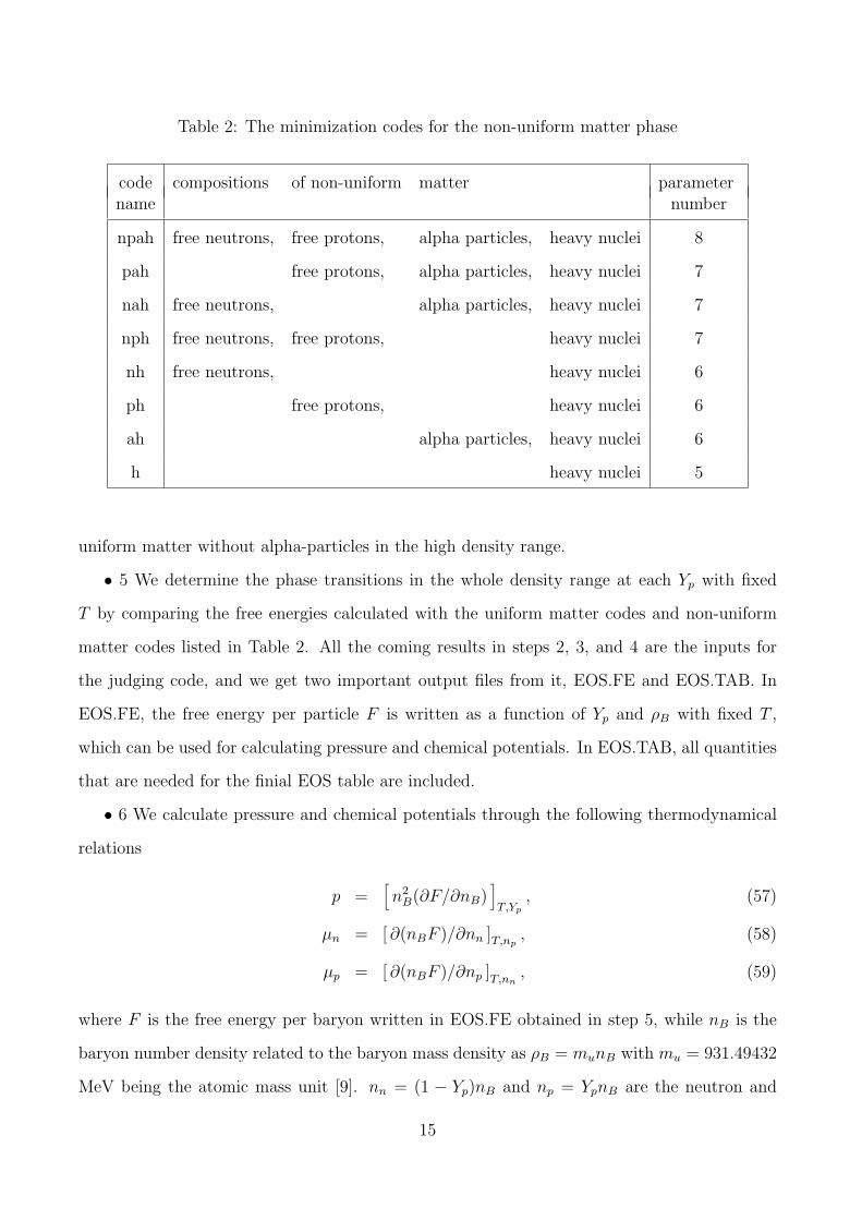
Table 2: The minimization codes for the non-uniform matter phase

code compositions of non-uniform matter parametername number

npah free neutrons, free protons, alpha particles, heavy nuclei 8

pah free protons, alpha particles, heavy nuclei 7

nah free neutrons, alpha particles, heavy nuclei 7

nph free neutrons, free protons, heavy nuclei 7

nh free neutrons, heavy nuclei 6

ph free protons, heavy nuclei 6

ah alpha particles, heavy nuclei 6

h heavy nuclei 5

uniform matter without alpha-particles in the high density range.

• 5 We determine the phase transitions in the whole density range at each Yp with fixed

T by comparing the free energies calculated with the uniform matter codes and non-uniform

matter codes listed in Table 2. All the coming results in steps 2, 3, and 4 are the inputs for

the judging code, and we get two important output files from it, EOS.FE and EOS.TAB. In

EOS.FE, the free energy per particle F is written as a function of Yp and ρB with fixed T ,

which can be used for calculating pressure and chemical potentials. In EOS.TAB, all quantities

that are needed for the finial EOS table are included.

• 6 We calculate pressure and chemical potentials through the following thermodynamical

relations

p =[n2

B(∂F/∂nB)]T,Yp

, (57)

µn = [ ∂(nBF )/∂nn ]T,np, (58)

µp = [ ∂(nBF )/∂np ]T,nn, (59)

where F is the free energy per baryon written in EOS.FE obtained in step 5, while nB is the

baryon number density related to the baryon mass density as ρB = munB with mu = 931.49432

MeV being the atomic mass unit [9]. nn = (1 − Yp)nB and np = YpnB are the neutron and

15

proton number densities, respectively. The numerical derivatives are calculated by a five-point

differentiation method. In the high density range where alpha-particles have been switched off,

we take the exact results calculated in the RMF theory instead of the numerical differentiations.

The output files of this step are PRE.TAB for pressure and CHE.TAB for chemical potentials.

• 7 We combine the files EOS.TAB, PRE.TAB, and CHE.TAB in order to get the finial

EOS table at this T . Due to the use of many codes listed in Table 2 for the non-uniform matter

phase, some fractions might be equal to zero at some densities in the file EOS.TAB. This is

because these compositions have been switched off for getting good accuracy. However, we

know that the fraction should be a small value at finite temperature if the chemical potential

is finite. In this case, we calculate the fraction Xi by the chemical potential µi and write it in

the finial EOS table,

Xi = (nouti V out)/(nBVcell), (60)

where Vcell is the cell volume as defined in Eq. (44), while V out = Vcell − 4π3

R3A is the volume

outside the heavy nucleus with RA being the maximum of Rp and Rn considered as the boundary

of the heavy nucleus. nouti is the free neutron number density (i = n) or free proton number

density (i = p). For alpha-particles (i = α), nouti should be four times of the alpha-particle

number density outside the heavy nucleus, because there are two protons and two neutrons in

an alpha-particle. The number densities outside the heavy nucleus can be obtained through

the relations,

noutn = 2

(MT

2π

)3/2

exp(µn

T), (61)

noutp = 2

(MT

2π

)3/2

exp(µp

T), (62)

noutα = 8

(MT

2π

)3/2

exp(µα + Bα

T), (63)

where µα = 2µn + 2µp is based on the equilibrium condition. The finial EOS table at this T is

the output file of this step.

We have to go through these steps for each T where the non-uniform matter phase exists. We

also add the results for zero temperature case (T = 0). There are two main differences between

T = 0 and T 6= 0 cases. (1) At T = 0, there are no alpha-particles and free protons (or free

16

neutrons) outside the heavy nucleus, so we need not calculate so many codes listed in Table 2.

The starting density of the non-uniform matter phase is below 105 g/cm3 at T < 0.4 MeV, so

we can skip step 2 in this case. (2) The ideal-gas approximation is not available at T = 0, so we

use a function Ck2f based on the Fermi-gas model to express the nonrelativistic kinetic energy

at low density. Note that the free energy at T = 0 is equal to the internal energy, because the

entropy is equal to zero in this case.

When the non-uniform matter phase disappears at high temperature, the calculation be-

comes relatively easy. We can skip step 3 which is the most complicated part in this calculation.

As the temperature increases, the alpha-particle contribution gets less and less. We actually

perform this uniform matter calculation depending on T . For T = 15 and 20 MeV, we still

use a large RMF input table as described in step 1 to calculate the mixed gas phase including

alpha-particles. When we write the finial EOS table, we switch off the alpha-particle contribu-

tion in the range of Xα < 10−4. For T = 25, 32, and 40 MeV, we use a small RMF input table

to calculate the fractions Xn, Xp, and Xα, while the alpha-particle contribution is neglected

in other quantities. Actually, the alpha-particle contribution is really small in this high tem-

perature range. As for T = 50, 63, 80, and 100 MeV, we only use a small RMF input table

to calculate Xα, while all other quantities are coming from the RMF results or the ideal-gas

approximation including antiparticles. The connection between the ideal-gas approximation

and the RMF theory is dependent on T , and we try to find out the density where they can be

connected with each other smoothly.

At the end, we calculate the pure neutron matter results (Yp = 0). There is only one com-

position in this case, so we can use the RMF theory to perform the calculation in the high

density range, while the ideal-gas approximation is used in the low density range. Finally, we

combine them to get the EOS table for Yp = 0.

6 Resulting EOS table

In this section, we explain the resulting EOS table and list the definitions of the physical

quantities tabulated. We provide the resulting EOS by three tables, which are named as

17

(1) eos1.tab (main EOS table, size: 53.21 MB)

• temperature T [MeV]: −1.0 ≤ log10(T ) ≤ 2.0; mesh of log10(T ) ' 0.1

• proton fraction Yp: −2.00 ≤ log10(Yp) ≤ −0.25; mesh of log10(Yp) = 0.025

• baryon mass density ρB [g/cm3]: 5.1 ≤ log10(ρB) ≤ 15.4; mesh of log10(ρB) ' 0.1

(2) eos1.t00 (EOS at T = 0, the same range of Yp and ρB, size: 1.72 MB)

(3) eos1.yp0 (EOS at Yp = 0, the same range of T and ρB, size: 0.78 MB)

One can download them from the following websites:

http://physics.nankai.edu.cn/grzy/shenhong/EOS/index.html

http://www.rcnp.osaka-u.ac.jp/∼shen/

In the model used in this calculation, we consider four compositions which are free neutrons,

free protons, alpha-particles, and a single species of heavy nuclei. Generally speaking, there are

two phases existing in the range covered by this EOS table. The phase where heavy nuclei are

formed is referred to as non-uniform matter, while the phase without heavy nuclei is referred

to as uniform matter. The phase transition can be found by the variation of the heavy nucleus

fraction between XA = 0 and XA 6= 0.

We write the EOS table in the following order: first fix T which is written at the beginning

of each block in the table, second fix Yp, third fix ρB. The blocks with different T are divided

by the string of characters ‘cccccccccccc’. For each T , Yp, and ρB, we write all quantities in one

line by the following order:

• (1) logarithm of baryon mass density: log10(ρB) [g/cm3]

• (2) baryon number density: nB [fm−3]

The baryon number density is related to the baryon mass density as ρB = munB with

mu = 931.49432 MeV being the atomic mass unit taken from Ref. [9].

• (3) logarithm of proton fraction: log10(Yp)

The proton fraction Yp of uniform matter is defined by

Yp =np + 2nα

nB

=np + 2nα

nn + np + 4nα

, (64)

18

where np is the proton number density, nn is the neutron number density, nα is the

alpha-particle number density, and nB is the baryon number density.

For non-uniform matter case, Yp is the average proton fraction defined by

Yp =Np

NB

, (65)

where Np is the proton number per cell, and NB is the baryon number per cell given by

Np =∫

cell[ np (r) + 2nα (r) ] d3r, (66)

NB =∫

cell[ nn (r) + np (r) + 4nα (r) ] d3r. (67)

Here, np(r) and nn(r) are the proton and neutron density distribution function given by

Eq. (45), and nα(r) is the alpha-particle density distribution function given by Eq. (47).

• (4) proton fraction: Yp

• (5) free energy per baryon: F [MeV]

The free energy per baryon is defined as relative to the free nucleon mass M = 938 MeV

in the TM1 parameter set as

F =f

nB

−M. (68)

• (6) internal energy per baryon: Eint [MeV]

The internal energy per baryon is defined as relative to the atomic mass unit mu =

931.49432 MeV as

Eint =ε

nB

−mu. (69)

• (7) entropy per baryon: S [kB]

The entropy per baryon is related to the entropy density via

S =s

nB

. (70)

• (8) mass number of the heavy nucleus: A

The mass number of the heavy nucleus is defined by

A =∫ RA

0[ nn (r) + np (r) ] 4πr2dr, (71)

19

where nn(r) and np(r) are the density distribution functions given by Eq. (45), and RA is

the maximum of Rp and Rn, which is considered as the boundary of the heavy nucleus.

• (9) charge number of the heavy nucleus: Z

The charge number of the heavy nucleus is defined by

Z =∫ RA

0np (r) 4πr2dr. (72)

• (10) effective nucleon mass: M∗ [MeV]

The effective nucleon mass is obtained in the RMF theory for uniform matter. In the

non-uniform matter phase, the effective nucleon mass is a function of space due to in-

homogeneity of the nucleon distribution, so it is meaningless to list the effective nucleon

mass for non-uniform matter. We replace the effective nucleon mass M∗ by the free

nucleon mass M in the non-uniform matter phase.

• (11) free neutron fraction: Xn

The free neutron fraction is given by

Xn = (noutn V out)/(nBVcell), (73)

where Vcell is the cell volume as defined in Eq. (44), V out = Vcell − 4π3

R3A is the volume

outside the heavy nucleus, noutn is the free neutron number density outside the heavy

nucleus, and nB is the average baryon number density.

• (12) free proton fraction: Xp

The free proton fraction is given by

Xp = (noutp V out)/(nBVcell), (74)

where noutp is the free proton number density outside the heavy nucleus.

• (13) alpha-particle fraction: Xα

The alpha-particle fraction is defined by

Xα = 4Nα/(nBVcell), (75)

20

where Nα is the alpha-particle number per cell obtained by

Nα =∫

cellnα (r) d3r, (76)

and nα(r) is the alpha-particle density distribution function given by Eq. (47).

• (14) heavy nucleus fraction: XA

The heavy nucleus fraction is defined by

XA = A/(nBVcell), (77)

where A is the mass number of the heavy nucleus as defined in Eq. (71).

• (15) pressure: p [MeV/fm3]

The pressure is calculated through the thermodynamical relation

p =[n2

B(∂F/∂nB)]T,Yp

. (78)

• (16) chemical potential of the neutron: µn [MeV]

The chemical potential of the neutron relative to the free nucleon mass M is calculated

through the thermodynamical relation

µn = [ ∂(nBF )/∂nn ]T,np. (79)

Here nn = (1− Yp) nB.

• (17) chemical potential of the proton: µp [MeV]

The chemical potential of the proton relative to the free nucleon mass M is calculated

through the thermodynamical relation

µp = [ ∂(nBF )/∂np ]T,nn. (80)

Here np = Yp nB.

We have done the following check for the EOS table:

(1) the consistency of the fractions,

Xn + Xp + Xα + XA = 1. (81)

21

(2) the consistency of the relation between F , Eint, and S,

F = Eint − TS + mu −M. (82)

(3) the consistency of the thermodynamical quantities,

F = µn(1− Yp) + µpYp − p

nB

. (83)

In general, these consistency relations can be satisfied within a few thousandths. Physical

constants to convert units are taken from Ref. [9].

7 Suggestions for using the EOS table

This relativistic EOS table is designed for use in supernova simulations, so we perform the

calculation at each T , Yp, and ρB. Note that the meshes of log10(T ) and log10(ρB) are not

exactly equal in the EOS table because of the difficulty in numerical calculation.

In order to perform the minimization of the free energy for non-uniform matter, we have

to parameterize the nucleon distributions, so that some quantities in the EOS table like A,

Z, Xn, Xp, Xα, and XA are dependent on this parameterization method. One should keep in

mind their definitions when these quantities are used. We suggest users pay more attention

to the thermodynamical quantities like F , Eint, S, p, µn, and µp, which are supposed not to

be sensitive to the parameterization method. The thermodynamical quantities are found to be

more smooth in the resulting EOS, while the use of many codes in Table 2 may bring some

fluctuations in the fractions, especially in the temperature range of 1 MeV < T < 5 MeV, where

the connection is very complicated.

We hope this EOS table can be used in your calculation successfully. We emphasize again

that this EOS table includes only baryon contributions, so you have to add the lepton contri-

butions when you use it.

References

[1] H. Shen, H. Toki, K. Oyamatsu, and K. Sumiyoshi, Prog. Theor. Phys. 100, 1013 (1998).

22

[2] H. Shen, H. Toki, K. Oyamatsu, and K. Sumiyoshi, Nucl. Phys. A637, 435 (1998).

[3] Y. Sugahara and H .Toki, Nucl. Phys. A579, 557 (1994).

[4] D. Hirata, K. Sumiyoshi, B. V. Carlson, H. Toki, and I. Tanihata, Nucl. Phys. A609,

131 (1996).

[5] K. Sumiyoshi, H. Kuwabara, and H. Toki, Nucl. Phys. A581, 725 (1995).

[6] B. D. Serot and J. D. Walecka, Adv. Nucl. Phys. 16, 1 (1986).

[7] J. M. Lattimer and F. D. Swesty, Nucl. Phys. A535, 331 (1991).

[8] K. Oyamatsu, Nucl. Phys. A561, 431 (1993).

[9] Physical Constants, Phys. Rev. D 50, 1233 (1994).

23