variability-resistant software through improved …mesl.ucsd.edu/site/talks/datecompiler13.pdf ·...

Variability-Resistant Software Through Improved Sensing & Modeling:

Compiler Directed Strategies

Rajesh K. Gupta

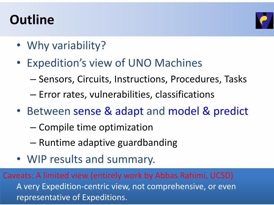
Outline

• Why variability?

• Expedition’s view of UNO Machines

– Sensors, Circuits, Instructions, Procedures, Tasks

– Error rates, vulnerabilities, classifications

• Between sense & adapt and model & predict

– Compile time optimization

– Runtime adaptive guardbanding

• WIP results and summary.

2

Caveats: A limited view (entirely work by Abbas Rahimi, UCSD) Caveats: A limited view (entirely work by Abbas Rahimi, UCSD) A very Expedition-centric view, not comprehensive, or even representative of Expeditions.

• Variability in transistor characteristics is a major challenge in nanoscale CMOS, PVTA – Static Process variation: effective transistor channel length and

threshold voltage – Dynamic variations: Temperature fluctuations, supply Voltage

droops, and device Aging (NBTI, HCI) • To handle variations designers use conservative guardbands

loss of operational efficiency

Variability is about Scale and Cost

22-Mar-13 3 Abbas Rahimi/ UC San Diego

Temperature

Clock

actual circuit delay guardband

Aging VCC Droop Across-wafer Frequency

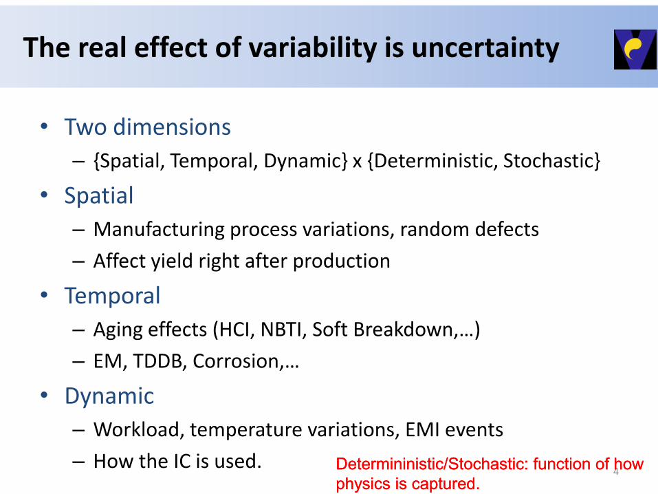
The real effect of variability is uncertainty

• Two dimensions

– {Spatial, Temporal, Dynamic} x {Deterministic, Stochastic}

• Spatial

– Manufacturing process variations, random defects

– Affect yield right after production

• Temporal

– Aging effects (HCI, NBTI, Soft Breakdown,…)

– EM, TDDB, Corrosion,…

• Dynamic

– Workload, temperature variations, EMI events

– How the IC is used. 4 DetermininisticDetermininistic/Stochastic: function of how /Stochastic: function of how

physics is captured.physics is captured.

Temporal and Functional Uncertainties

• Temporal uncertainties are quite familiar to real-time systems community – Measures that span architectural simplification to OS simplification,

structuring computation as precise and imprecise and combining with real-time OS models (FG/BG).

• PL: from performance to correctness to reliability

• Lately PL community has taken on fault-tolerant computations – How to avoid BSD? Decompose, Calibrate, Acceptance Tests

– Probabilistic Accuracy Bound & Early Phase Termination, [Rinard, ICS 2006]

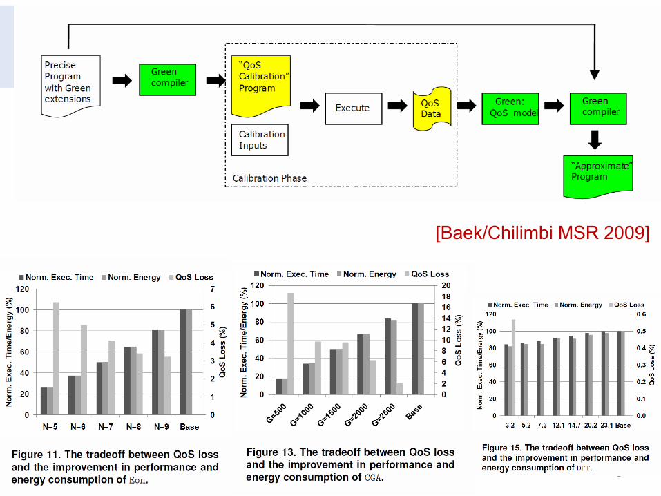
– Principled Approximation [Baek/Chilimbi MSR 2009]

• Programmer approximates expensive functions, build a model of QOS loss by the approximation during calibration phase – Use model during operational phase to save energy by an adaptation

function that monitors runtime behavior.

5

6

[Baek/Chilimbi MSR 2009]

Closer to HW: Uncertainty Manifestations

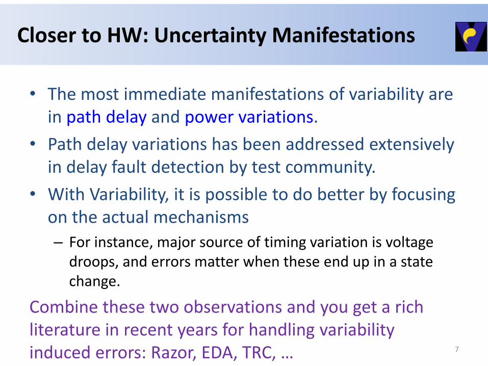
• The most immediate manifestations of variability are in path delay and power variations.

• Path delay variations has been addressed extensively in delay fault detection by test community.

• With Variability, it is possible to do better by focusing on the actual mechanisms

– For instance, major source of timing variation is voltage droops, and errors matter when these end up in a state change.

Combine these two observations and you get a rich literature in recent years for handling variability induced errors: Razor, EDA, TRC, … 7

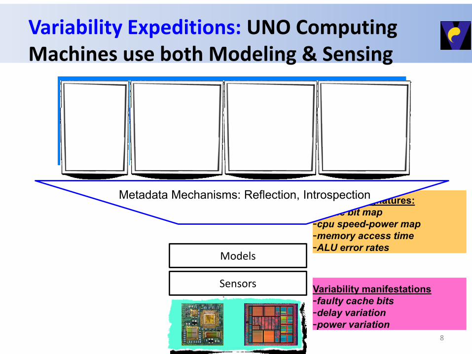
Variability Expeditions: UNO Computing Machines use both Modeling & Sensing

Variability manifestations

-faulty cache bits

-delay variation

-power variation

Variability manifestations

-faulty cache bits

-delay variation

-power variation

Variability signatures:

-cache bit map

-cpu speed-power map

-memory access time

-ALU error rates

Variability signatures:

-cache bit map

-cpu speed-power map

-memory access time

-ALU error rates

Do Nothing

(Elastic User,

Robust App)

Change

Algorithm

Parameters

(Codec Setting,

Duty Cycle Ratio)

Change

Algorithm

Implementation

(Alternate code

path, Dynamic

recompilation)

Change Hardware

Operating Point

(Disabling parts of

the cache,

Changing V-f)

8

Sensors

Models

Metadata Mechanisms: Reflection, Introspection

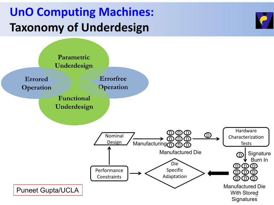
UnO Computing Machines: Taxonomy of Underdesign

9

Nominal Design

Hardware Characterization

Tests

Die Specific

Adaptation

D

Signature

Burn In

Manufacturing

Manufactured Die

Performance Constraints

D D D

D D D

D D D

D D D

D D D

D D D

D

Manufactured Die

With Stored

Signatures

Puneet Gupta/UCLA

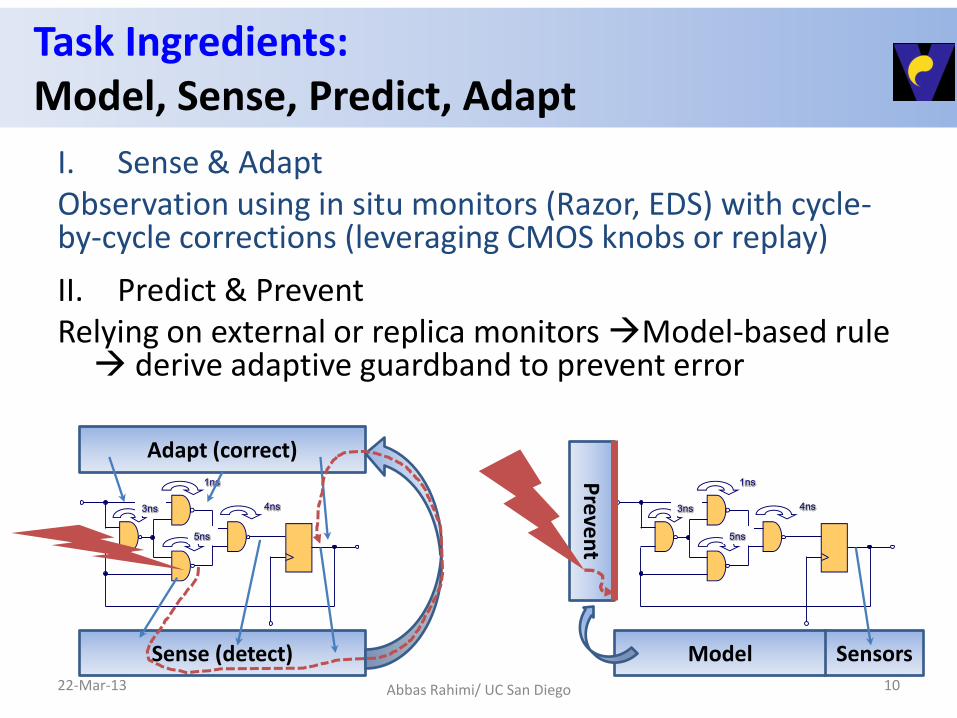
Task Ingredients: Model, Sense, Predict, Adapt

I. Sense & Adapt Observation using in situ monitors (Razor, EDS) with cycle-by-cycle corrections (leveraging CMOS knobs or replay)

22-Mar-13 Abbas Rahimi/ UC San Diego 10

1ns

4ns3ns

5ns

Sense (detect)

Adapt (correct)

Sensors Model

1ns

4ns3ns

5ns

Preve

nt

II. Predict & Prevent Relying on external or replica monitors Model-based rule derive adaptive guardband to prevent error

Instruction-level Vulnerability (ILV)

Sequence-level Vulnerability (SLV)

Procedure-level Vulnerability (PLV)

Task-level Vulnerability (TLV)

Monitor manifestations from instructions levels to task levels.

Expedition View of Cross-layer Awarenes & Adaptation (cf.: memory model)

By the time, we get to TLV, we are into a parallel software context: instruct OpenMP scheduler, even create an abstraction for programmers to express irregular and unstructured parallelism (code refactoring).

The steps to build

variability abstractions

up to the SW layer

Methodology

• Characterize effects of Dynamic Voltage and Temperature

Variation

• Estimate their effects on instruction executions

– Instruction-level Vulnerability (ILV)

– Sequence-level Vulnerability (SLV)

• Classify instructions, and sequences of instructions

• Use ILV, SLV

– Compile time optimization

– Runtime adaptive guardbanding

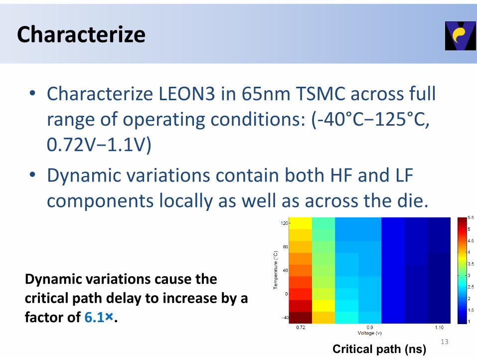
Characterize

• Characterize LEON3 in 65nm TSMC across full range of operating conditions: (-40°C−125°C, 0.72V−1.1V)

• Dynamic variations contain both HF and LF components locally as well as across the die.

13

Critical path (ns)

Dynamic variations cause the critical path delay to increase by a factor of 6.1×.

WAIT! DID WE MISS A STEP? One First Challenge: How do we make the leap to Software?

14

0

2

4

6

8

10

12

14

16

Fetch Decode Reg. acc. Execute Memory Write back

Num

ber

of

faile

d p

ath

s

x 10000 0.72V 0.88V 1.10V

0

1

2

3

4

5

6

7

8

Fetch Decode Reg. acc. Execute Memory Write back

Num

ber

of

faile

d p

ath

s

x 10000 -40 C 0 C 125 C

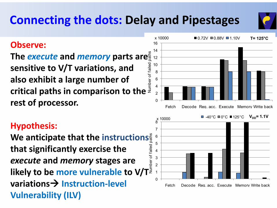
Observe: The execute and memory parts are sensitive to V/T variations, and also exhibit a large number of critical paths in comparison to the rest of processor. Hypothesis: We anticipate that the instructions that significantly exercise the execute and memory stages are likely to be more vulnerable to V/T variations Instruction-level Vulnerability (ILV)

VDD= 1.1V

T= 125°C

Connecting the dots: Delay and Pipestages

Method for ISA-level & Sequence-level Characterization

• For SPARC V8 instructions (V, T, F) are varied and – ILVi is evaluated for every instructioni with random operands

– SLVi is evaluated for a high-frequent sequencei of instructions

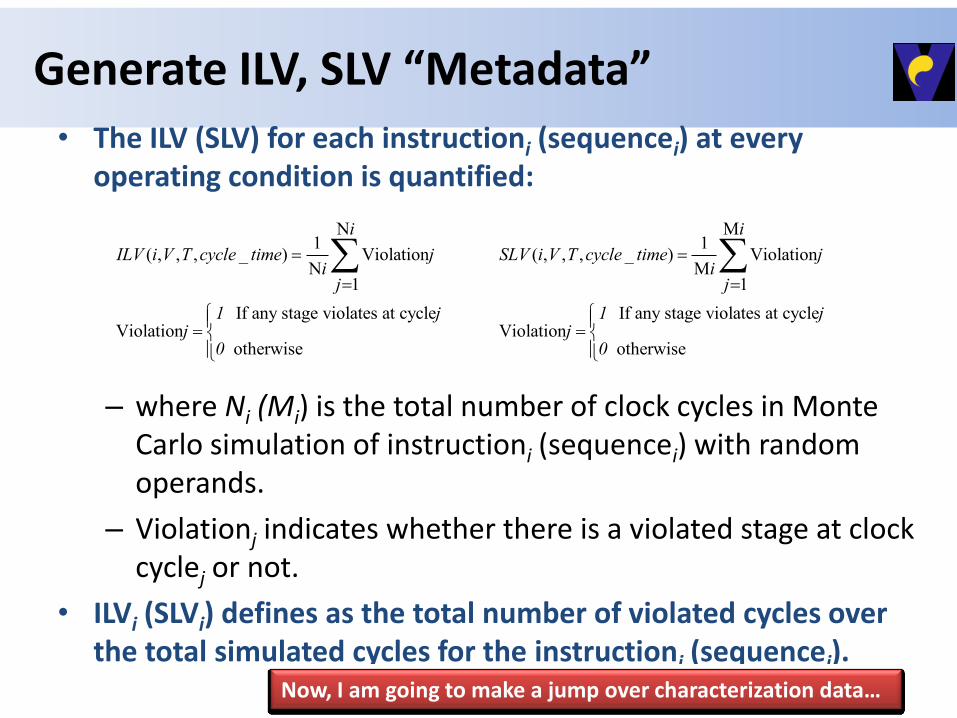
Generate ILV, SLV “Metadata” • The ILV (SLV) for each instructioni (sequencei) at every

operating condition is quantified:

– where Ni (Mi) is the total number of clock cycles in Monte Carlo simulation of instructioni (sequencei) with random operands.

– Violationj indicates whether there is a violated stage at clock cyclej or not.

• ILVi (SLVi) defines as the total number of violated cycles over the total simulated cycles for the instructioni (sequencei).

M1

( , , , _ ) ViolationM

1

If any stage violates at cycleViolation

otherwise

i

SLV i V T cycle time jij

1 jj

0

N

1( , , , _ ) Violation

N1

If any stage violates at cycleViolation

otherwise

i

ILV i V T cycle time jij

1 jj

0

Now, I am going to make a jump over characterization data…

1 Classify Instructions in 3 Classes

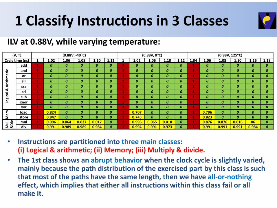
• Instructions are partitioned into three main classes: (i) Logical & arithmetic; (ii) Memory; (iii) Multiply & divide.

• The 1st class shows an abrupt behavior when the clock cycle is slightly varied, mainly because the path distribution of the exercised part by this class is such that most of the paths have the same length, then we have all-or-nothing effect, which implies that either all instructions within this class fail or all make it.

(V, T) (0.88V, -40°C) (0.88V, 0°C) (0.88V, 125°C)

Cycle time (ns) 1 1.02 1.06 1.08 1.10 1.12 1 1.02 1.06 1.10 1.12 1.04 1.06 1.08 1.10 1.16 1.18

Logi

cal &

Ari

thm

etic

add 1 0 0 0 0 0 1 0 0 0 0 1 0 0 0 0 0

and 1 0 0 0 0 0 1 0 0 0 0 1 0 0 0 0 0

or 1 0 0 0 0 0 1 0 0 0 0 1 0 0 0 0 0

sll 1 0 0 0 0 0 1 0 0 0 0 1 0 0 0 0 0

sra 1 0 0 0 0 0 1 0 0 0 0 1 0 0 0 0 0

srl 1 0 0 0 0 0 1 0 0 0 0 1 0 0 0 0 0

sub 1 0 0 0 0 0 1 0 0 0 0 1 0 0 0 0 0

xnor 1 0 0 0 0 0 1 0 0 0 0 1 0 0 0 0 0 xor 1 0 0 0 0 0 1 0 0 0 0 1 0 0 0 0 0

Me

m

load 1 0.824 0 0 0 0 1 0.707 0 0 0 1 0.796 0 0 0 0 store 1 0.847 0 0 0 0 1 0.743 0 0 0 1 0.823 0 0 0 0

Mu

l.&

Div

mul 1 0.996 0.064 0.027 0.017 0 1 0.996 0.065 0.018 0 1 0.876 0.876 0.016 06 0 div 1 0.991 0.989 0.989 0.984 0 1 0.994 0.991 0.973 0 1 0.991 0.991 0.991 0.984 0

ILV at 0.88V, while varying temperature:

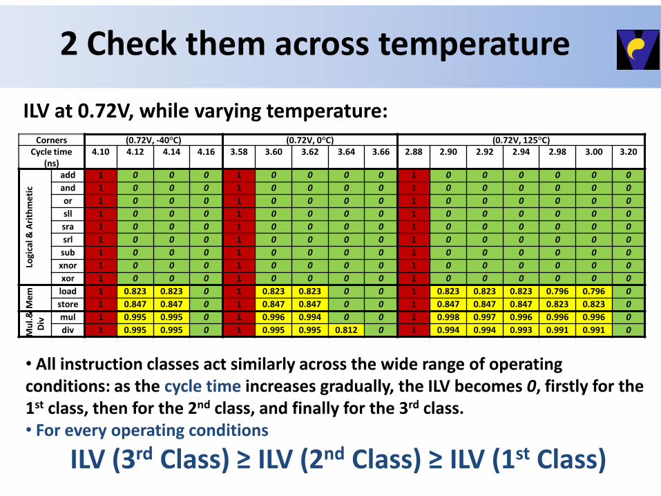
2 Check them across temperature

Corners (0.72V, -40°C) (0.72V, 0°C) (0.72V, 125°C) Cycle time

(ns) 4.10 4.12 4.14 4.16 3.58 3.60 3.62 3.64 3.66 2.88 2.90 2.92 2.94 2.98 3.00 3.20

Logi

cal &

Ari

thm

eti

c

add 1 0 0 0 1 0 0 0 0 1 0 0 0 0 0 0

and 1 0 0 0 1 0 0 0 0 1 0 0 0 0 0 0

or 1 0 0 0 1 0 0 0 0 1 0 0 0 0 0 0

sll 1 0 0 0 1 0 0 0 0 1 0 0 0 0 0 0

sra 1 0 0 0 1 0 0 0 0 1 0 0 0 0 0 0

srl 1 0 0 0 1 0 0 0 0 1 0 0 0 0 0 0

sub 1 0 0 0 1 0 0 0 0 1 0 0 0 0 0 0

xnor 1 0 0 0 1 0 0 0 0 1 0 0 0 0 0 0

xor 1 0 0 0 1 0 0 0 0 1 0 0 0 0 0 0

Me

m

load 1 0.823 0.823 0 1 0.823 0.823 0 0 1 0.823 0.823 0.823 0.796 0.796 0

store 1 0.847 0.847 0 1 0.847 0.847 0 0 1 0.847 0.847 0.847 0.823 0.823 0

Mu

l.&

Div

mul 1 0.995 0.995 0 1 0.996 0.994 0 0 1 0.998 0.997 0.996 0.996 0.996 0

div 1 0.995 0.995 0 1 0.995 0.995 0.812 0 1 0.994 0.994 0.993 0.991 0.991 0

ILV at 0.72V, while varying temperature:

• All instruction classes act similarly across the wide range of operating conditions: as the cycle time increases gradually, the ILV becomes 0, firstly for the 1st class, then for the 2nd class, and finally for the 3rd class. • For every operating conditions

ILV (3rd Class) ≥ ILV (2nd Class) ≥ ILV (1st Class)

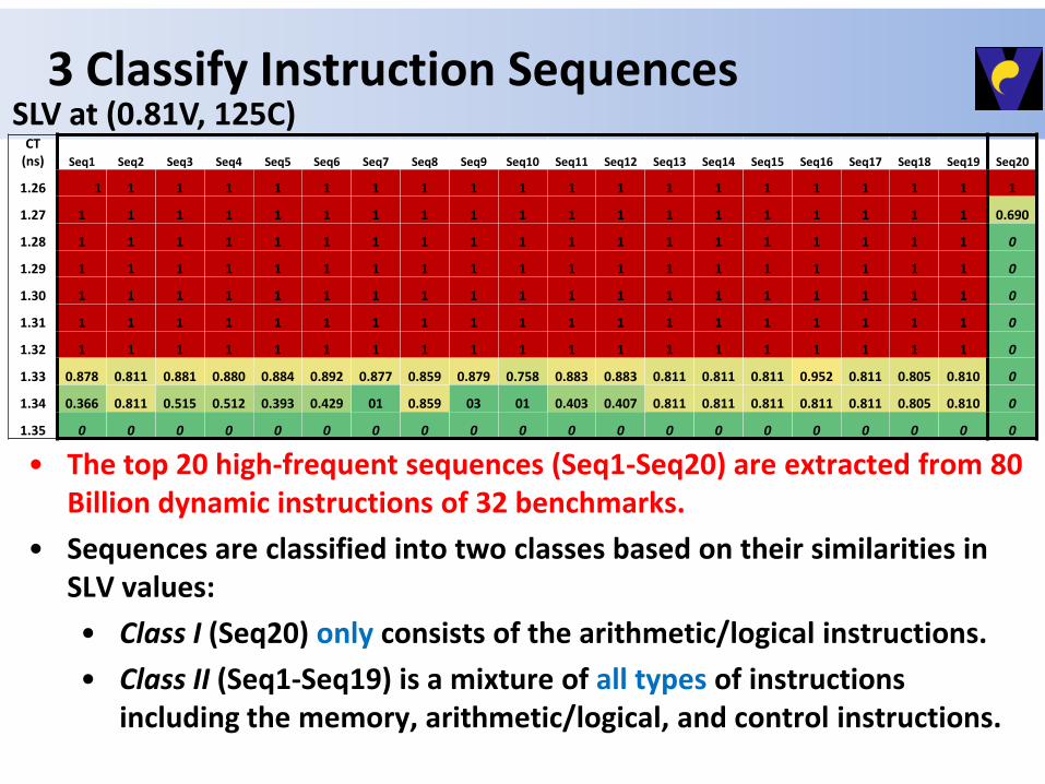
3 Classify Instruction Sequences CT

(ns) Seq1 Seq2 Seq3 Seq4 Seq5 Seq6 Seq7 Seq8 Seq9 Seq10 Seq11 Seq12 Seq13 Seq14 Seq15 Seq16 Seq17 Seq18 Seq19 Seq20

1.26 1 1 1 1 1 1 1 1 1 1 1 1 1 1 1 1 1 1 1 1

1.27 1 1 1 1 1 1 1 1 1 1 1 1 1 1 1 1 1 1 1 0.690

1.28 1 1 1 1 1 1 1 1 1 1 1 1 1 1 1 1 1 1 1 0

1.29 1 1 1 1 1 1 1 1 1 1 1 1 1 1 1 1 1 1 1 0

1.30 1 1 1 1 1 1 1 1 1 1 1 1 1 1 1 1 1 1 1 0

1.31 1 1 1 1 1 1 1 1 1 1 1 1 1 1 1 1 1 1 1 0

1.32 1 1 1 1 1 1 1 1 1 1 1 1 1 1 1 1 1 1 1 0

1.33 0.878 0.811 0.881 0.880 0.884 0.892 0.877 0.859 0.879 0.758 0.883 0.883 0.811 0.811 0.811 0.952 0.811 0.805 0.810 0

1.34 0.366 0.811 0.515 0.512 0.393 0.429 01 0.859 03 01 0.403 0.407 0.811 0.811 0.811 0.811 0.811 0.805 0.810 0

1.35 0 0 0 0 0 0 0 0 0 0 0 0 0 0 0 0 0 0 0 0

SLV at (0.81V, 125C)

• The top 20 high-frequent sequences (Seq1-Seq20) are extracted from 80 Billion dynamic instructions of 32 benchmarks.

• Sequences are classified into two classes based on their similarities in SLV values:

• Class I (Seq20) only consists of the arithmetic/logical instructions.

• Class II (Seq1-Seq19) is a mixture of all types of instructions including the memory, arithmetic/logical, and control instructions.

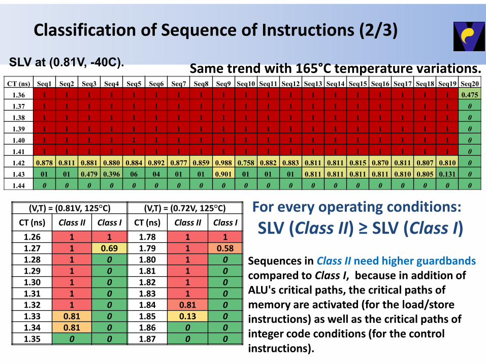
Classification of Sequence of Instructions (2/3)

CT (ns) Seq1 Seq2 Seq3 Seq4 Seq5 Seq6 Seq7 Seq8 Seq9 Seq10 Seq11 Seq12 Seq13 Seq14 Seq15 Seq16 Seq17 Seq18 Seq19 Seq20

1.36 1 1 1 1 1 1 1 1 1 1 1 1 1 1 1 1 1 1 1 0.475

1.37 1 1 1 1 1 1 1 1 1 1 1 1 1 1 1 1 1 1 1 0

1.38 1 1 1 1 1 1 1 1 1 1 1 1 1 1 1 1 1 1 1 0

1.39 1 1 1 1 1 1 1 1 1 1 1 1 1 1 1 1 1 1 1 0

1.40 1 1 1 1 1 1 1 1 1 1 1 1 1 1 1 1 1 1 1 0

1.41 1 1 1 1 1 1 1 1 1 1 1 1 1 1 1 1 1 1 1 0

1.42 0.878 0.811 0.881 0.880 0.884 0.892 0.877 0.859 0.988 0.758 0.882 0.883 0.811 0.811 0.815 0.870 0.811 0.807 0.810 0

1.43 01 01 0.479 0.396 06 04 01 01 0.901 01 01 01 0.811 0.811 0.811 0.811 0.810 0.805 0.131 0

1.44 0 0 0 0 0 0 0 0 0 0 0 0 0 0 0 0 0 0 0 0

SLV at (0.81V, -40C). Same trend with 165°C temperature variations.

(V,T) = (0.81V, 125°C) (V,T) = (0.72V, 125°C)

CT (ns) Class II Class I CT (ns) Class II Class I

1.26 1 1 1.78 1 1 1.27 1 0.69 1.79 1 0.58 1.28 1 0 1.80 1 0 1.29 1 0 1.81 1 0 1.30 1 0 1.82 1 0 1.31 1 0 1.83 1 0 1.32 1 0 1.84 0.81 0 1.33 0.81 0 1.85 0.13 0 1.34 0.81 0 1.86 0 0 1.35 0 0 1.87 0 0

For every operating conditions:

SLV (Class II) ≥ SLV (Class I)

Sequences in Class II need higher guardbands compared to Class I, because in addition of ALU's critical paths, the critical paths of memory are activated (for the load/store instructions) as well as the critical paths of integer code conditions (for the control instructions).

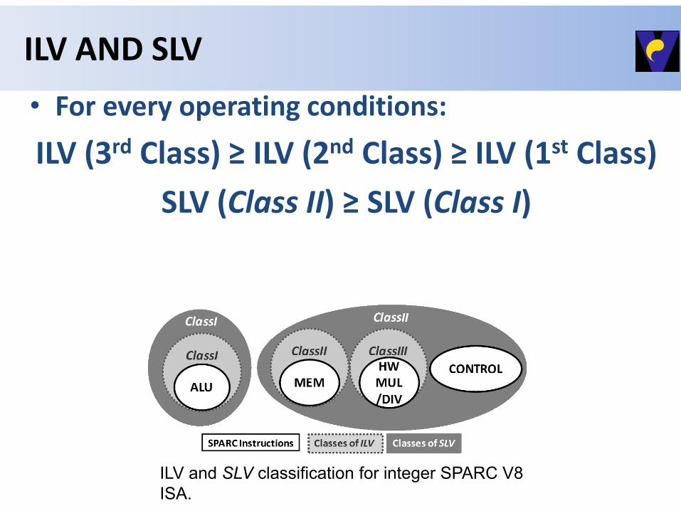
• For every operating conditions:

ILV (3rd Class) ≥ ILV (2nd Class) ≥ ILV (1st Class)

SLV (Class II) ≥ SLV (Class I)

ILV and SLV classification for integer SPARC V8

ISA.

ILV AND SLV

Now Use ILV, SLV

VA Compiler

Application Code

SLV

ILV

App.

type

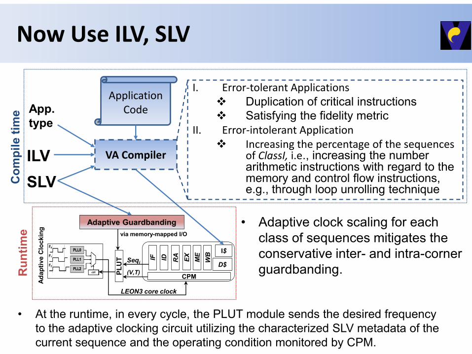
I. Error-tolerant Applications

Duplication of critical instructions

Satisfying the fidelity metric II. Error-intolerant Application

Increasing the percentage of the sequences of ClassI, i.e., increasing the number arithmetic instructions with regard to the memory and control flow instructions, e.g., through loop unrolling technique

Adaptive Guardbanding

IF

ID

WB

CPM

I$

D$

PL

UT

RA

EX

ME

Ad

ap

tiv

e C

lockin

g

(V,T)

Seqi

via memory-mapped I/O

LEON3 core clock

Co

mp

ile t

ime

Ru

nti

me • Adaptive clock scaling for each

class of sequences mitigates the

conservative inter- and intra-corner

guardbanding.

• At the runtime, in every cycle, the PLUT module sends the desired frequency

to the adaptive clocking circuit utilizing the characterized SLV metadata of the

current sequence and the operating condition monitored by CPM.

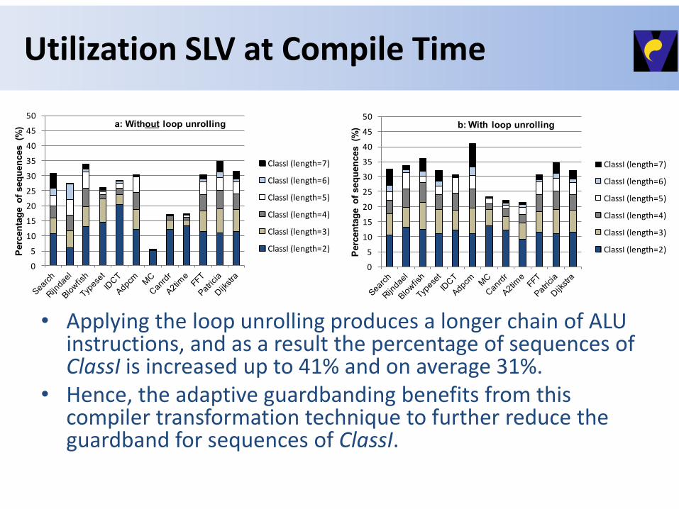
Utilization SLV at Compile Time

• Applying the loop unrolling produces a longer chain of ALU instructions, and as a result the percentage of sequences of ClassI is increased up to 41% and on average 31%.

• Hence, the adaptive guardbanding benefits from this compiler transformation technique to further reduce the guardband for sequences of ClassI.

0

5

10

15

20

25

30

35

40

45

50

Perc

en

tag

e o

f seq

uen

ces (%

) a: Without loop unrolling

ClassI (length=7)

ClassI (length=6)

ClassI (length=5)

ClassI (length=4)

ClassI (length=3)

ClassI (length=2)

0

5

10

15

20

25

30

35

40

45

50

Perc

en

tag

e o

f seq

uen

ces (%

) b: With loop unrolling

ClassI (length=7)

ClassI (length=6)

ClassI (length=5)

ClassI (length=4)

ClassI (length=3)

ClassI (length=2)

Effectiveness of Adaptive Guardbanding

• Using online SLV coupled with offline compiler techniques enables the processor to achieve 1.6× average speedup for intolerant applications, compared to recent work [Hoang’11], by adapting the cycle time for dynamic variations (inter-corner) and different instruction sequences (intra-corner).

1.2

1.3

1.4

1.5

1.6

1.7

1.8

1.9

No

rmali

zed

Th

rou

gh

pu

t

(0.72V,125°) (0.81V,0°) (0.81V,125°)

0.80

1.00

1.20

1.40

1.60

1.80

2.00

No

rmali

zed

Th

rou

gh

pu

t

(0.72V,125°) (0.81V,0°) (0.81V,125°)

• Adaptive guardbanding achieves up to 1.9× performance improvement for error-tolerant (probabilistic) applications in comparison to the traditional worst-case design.

[Hoang’11] G. Hoang, et al., "Exploring circuit timing-aware language and compilation,“ ASPLOS, 2011.

Example: Procedure Hopping in Clustered CPU, Each core with its voltage domain

• Statically characterize procedure for PLV

• A core increases voltage if monitored delay is high

• A procedure hops from one core to another if its voltage variation is high

• Less 1% cycle overhead in EEMBC.

26

... I$Bi-1I$B0

Log. Interc.

Core15

VA

-VD

D-h

op

pin

g

... TCDMBj-1TCDMB0

Log. Interc.

Low VDD

Typical VDD

High VDD

DF

S...

f+1

80

°f+

18

0°

f

CPM

Level ShiftersLevel Shifters

Level ShiftersLevel Shifters

SHM

PSS

Core0

VA

-VD

D-h

op

pin

g

CPM

PSS

VDD = 0.81V VDD = 0.99V VA-VDD-Hopping=( 0.81V 0.99V , )

f0

862

f1

909

f2

870

f3

847

f4

826

f5

855

f6

877

f7

893

f8

820

f9

826

f10

909

f11

847

f12

901

f13

917

f14

847

f15

901

f0

862

f1

909

f2

870

f3

847

f4

1370

f5

855

f6

877

f7

893

f8

1370

f9

1370

f10

909

f11

847

f12

901

f13

917

f14

847

f15

901

f0

1408

f1

1389

f2

1408

f3

1370

f4

1370

f5

1408

f6

1408

f7

1408

f8

1370

f9

1370

f10

1389

f11

1370

f12

1408

f13

1408

f14

1389

f15

1389

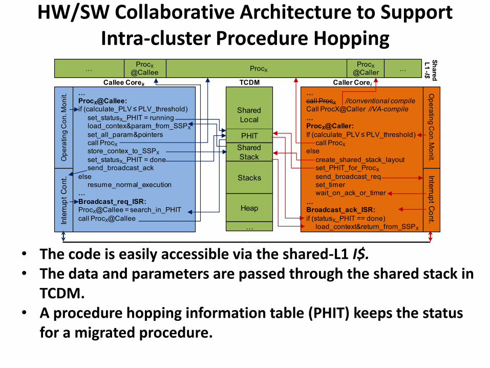
HW/SW Collaborative Architecture to Support Intra-cluster Procedure Hopping

27

• The code is easily accessible via the shared-L1 I$. • The data and parameters are passed through the shared stack in

TCDM. • A procedure hopping information table (PHIT) keeps the status

for a migrated procedure.

…ProcX@Callee:if (calculate_PLV ≤ PLV_threshold)

set_statusX_PHIT = runningload_contex&param_from_SSPX

set_all_param&pointerscall ProcX

store_contex_to_SSPX

set_statusX_PHIT = donesend_broadcast_ack

else resume_normal_execution

…

Broadcast_req_ISR:ProcX@Callee = search_in_PHIT

call ProcX@Callee

…call ProcX //conventional compile Call ProcX@Caller //VA-compile

…ProcX@Caller:

If (calculate_PLV ≤ PLV_threshold)call ProcX

else

create_shared_stack_layoutset_PHIT_for_ProcX

send_broadcast_reqset_timerwait_on_ack_or_timer

…Broadcast_ack_ISR:

if (statusX_PHIT == done)load_context&return_from_SSPX

Shared

Local

Heap

Shared

Stack

ProcXProcX

@Callee

PHIT

Op

era

ting

Co

n. M

on

it.In

terru

pt C

ont.

Op

era

tin

g C

on

. Mo

nit.

Inte

rrup

t C

ont.

TCDM

Sh

are

d

L1 -I$

Callee Corek Caller Corei

ProcX

@Caller……

…

Stacks

NOT SURE HOW FAR WE CAN PUSH THIS SENSING. REMEMBER ILP?

Towards Model and Predict

28

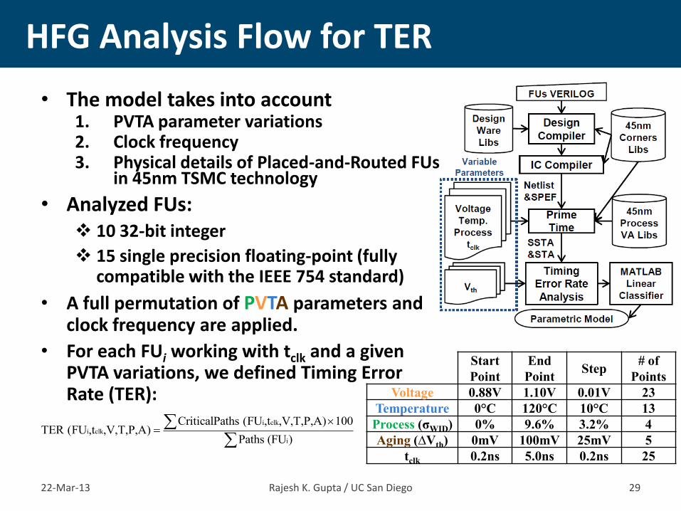
• The model takes into account 1. PVTA parameter variations 2. Clock frequency 3. Physical details of Placed-and-Routed FUs

in 45nm TSMC technology

• Analyzed FUs: 10 32-bit integer

15 single precision floating-point (fully compatible with the IEEE 754 standard)

• A full permutation of PVTA parameters and clock frequency are applied.

• For each FUi working with tclk and a given PVTA variations, we defined Timing Error Rate (TER):

HFG Analysis Flow for TER

22-Mar-13 Rajesh K. Gupta / UC San Diego 29

Start

Point

End

Point Step

# of

Points

Voltage 0.88V 1.10V 0.01V 23

Temperature 0°C 120°C 10°C 13

Process (σWID) 0% 9.6% 3.2% 4

Aging (∆Vth) 0mV 100mV 25mV 5

tclk 0.2ns 5.0ns 0.2ns 25

i clk

i clk

i

CriticalPaths (FU ,t ,V,T,P,A) 100TER (FU ,t ,V,T,P,A)

Paths (FU )

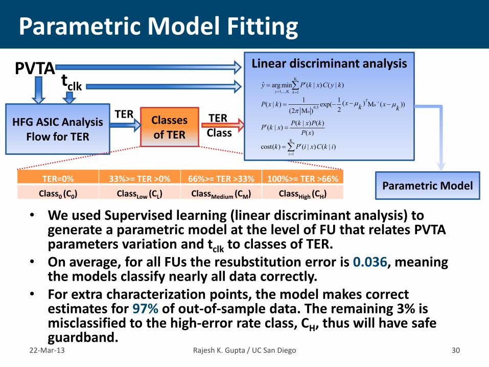
• We used Supervised learning (linear discriminant analysis) to generate a parametric model at the level of FU that relates PVTA parameters variation and tclk to classes of TER.

• On average, for all FUs the resubstitution error is 0.036, meaning the models classify nearly all data correctly.

• For extra characterization points, the model makes correct estimates for 97% of out-of-sample data. The remaining 3% is misclassified to the high-error rate class, CH, thus will have safe guardband.

Parametric Model Fitting


HFG ASIC Analysis Flow for TER

PVTA tclk

TER=0% 33%>= TER >0% 66%>= TER >33% 100%>= TER >66%

Class0 (C0) ClassLow (CL) ClassMedium (CM) ClassHigh (CH)

Classes of TER

TER TER Class

K

1,...,K 1

ˆ ( | ) ( | )arg miny k

y P k x C y k

1σ

0.5σ

1 1( )( | ) exp( M ( ))

2(2 M )

TxP x k xk k

( | ) ( )( | )

( )

P k x P kP k x

P x

K

1

cost( ) ( | ) ( | )i

k P i x C k i

Linear discriminant analysis

Parametric Model

• During design time the delay of the FP adder has a large uncertainty of [0.73ns,1.32ns], since the actual values of PVTA parameters are unknown.

Delay Variation and TER Characterization


(P,?,?,?) (P,A,?,?) (P,A,T,?)(P,A,T,V)

P(σWID)=

0%

A(∆Vth)=

0mV

T=0°C

V=1.10V

…

V=0.88V

… …

T=120°C

V=1.10V

…

V=0.88V

… … …

A(∆Vth)=

100mV

T=0°C

V=1.10V

…

V=0.88V

… …

T=120°C

V=1.10V

…

V=0.88V

… … … …

P(σWID)=

9.6%

A(∆Vth)=

0mV

T=0°C

V=1.10V

…

V=0.88V

…

T=120°C

V=1.10V

…

V=0.88V

… … …

A(∆Vth)=

100mV

T=0°C

V=1.10V

…

V=0.88V

… …

T=120°C

V=1.10V

…

V=0.88V

Delay

(ns)

0

50

100

0.90.95

11.05

1.1

0

20

40

60

80

100

Temperature (°C)VDD (V)

Tim

ing

Err

or

Ra

te (

%)

20

40

60

80

0

50

100

0.90.95

11.05

1.1

0

20

40

60

80

100

Temperature (°C)

VDD (V)

Tim

ing

Err

or

Ra

te (

%)

0

20

40

60

80

(P(σWID) = 0%, A(∆Vth)=100mV)

(P(σWID) = 0%, A(∆Vth)=0mV)

0

50

100

0.9

0.95

1

1.05

1.1

0

20

40

60

80

100


Tim

ing

Err

or

Ra

te (

%)

0

20

40

60

80

(P(σWID) = 9.6%, A(∆Vth)=0mV)

020

4060

80100

120

0.9

0.95

1

1.05

1.1

0

20

40

60

80

100


Tim

ing

Err

or

Ra

te (

%)

20

40

60

80

(P(σWID) = 9.6%, A(∆Vth)=100mV)

• The question is that mix of monitors that would be useful?

• The more sensors we provide for a FU, the better conservative guardband reduction for that FU.

Hierarchical Sensors Observability


0.6

0.8

1.0

1.2

1.4

1.6

1.8

2.0

2.2

2.4

2.6t c

lk(n

s)

FP_expFP_add

INT_mac

P_sensor PA_sensors PAT_sensors PATV_sensors • The guardband of FP adder can be reduced up to • 8% (P_sensor),

• 24% (PA_sensors),

• 28% (PAT_sensors),

• 44% (PATV_sensors)

Sensor overheads: In-situ PVT sensors impose 1−3% area overhead [Bowman’09] Five replica PVT sensors increase area of by 0.2% [Lefurgy’11] The banks of 96 NBTI aging sensors occupy less than 0.01% of the core's area [Singh’11]

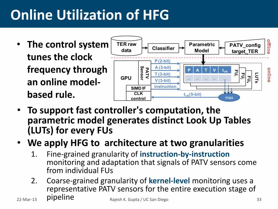
• The control system tunes the clock frequency through an online model-based rule.

Online Utilization of HFG


FU

k

FU

j

TER raw

data ClassifierParametric

ModelPATV_config

target_TER

P A T V tclk

… … … … …

PA

TV

Sen

so

r

CLK

control

FU

i

max

P (2-bit)

A (3-bit)

T (3-bit)

V (3-bit)

instruction

tclk(5-bit)

LU

TsGPU

SIMD IF

offlin

eo

nlin

e

• To support fast controller's computation, the parametric model generates distinct Look Up Tables (LUTs) for every FUs

• We apply HFG to architecture at two granularities 1. Fine-grained granularity of instruction-by-instruction

monitoring and adaptation that signals of PATV sensors come from individual FUs

2. Coarse-grained granularity of kernel-level monitoring uses a representative PATV sensors for the entire execution stage of pipeline

Throughput benefit of HFG


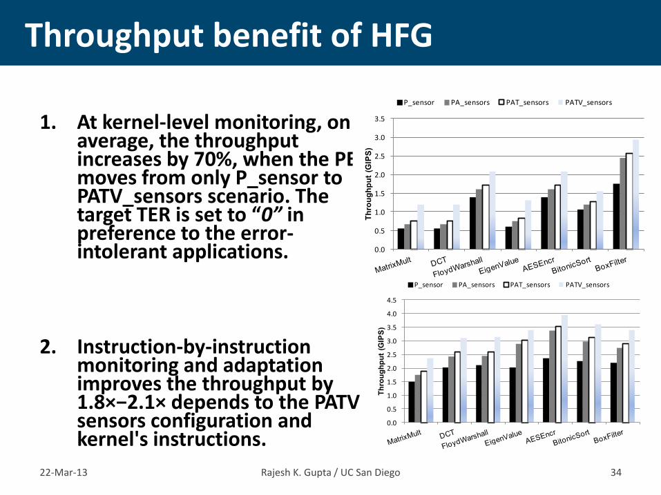
1. At kernel-level monitoring, on

average, the throughput increases by 70%, when the PE moves from only P_sensor to PATV_sensors scenario. The target TER is set to “0” in preference to the error-intolerant applications.

2. Instruction-by-instruction monitoring and adaptation improves the throughput by 1.8×−2.1× depends to the PATV sensors configuration and kernel's instructions.

0.0

0.5

1.0

1.5

2.0

2.5

3.0

3.5

Th

rou

gh

pu

t (G

IPS

)

P_sensor PA_sensors PAT_sensors PATV_sensors

0.0

0.5

1.0

1.5

2.0

2.5

3.0

3.5

4.0

4.5

Th

rou

gh

pu

t (G

IPS

)

P_sensor PA_sensors PAT_sensors PATV_sensors

Thank You!

35

http://variability.org

The Variability Expedition

A NSF Expeditions in Computing Project

variability-resistant software through improved …mesl.ucsd.edu/site/talks/datecompiler13.pdf ·...

Documents