������������ ��������������������������������������������������������������� �!"�"""��������

Research Memorandum GD-49

Harry X. Wu

Groningen Growth and Development CentreJuly 2001

������������ ��������������������������������������������������������������� �!"�"""���������#

Harry X. Wu**

Department of Business StudiesThe Hong Kong Polytechnic University, Hong Kong

ABSTRACT

This study joins the debate of whether Chinese manufacturing has experienced asignificant catch-up with or a process of falling behind the world’s advancedeconomies. It calculates a new set of industry-of-origin China-US PPPs for majormanufacturing industries at 1987 prices. Then using a newly constructed data set, itderives China’s comparative labour productivity level in manufacturing for 1952-97.The results show that China’s comparative labour productivity increased from about3.0 in 1952 to 7.6 in 1997 (USA=100), but with a long stagnation at around 4.5between 1958 and 1990. A clear catch-up process has been observed since the 1990swhen China’s market-oriented reform deepened.

������������� : F31, L60, O47, P27

��������: Industry-of-origin purchasing power parity, Comparative labourproductivity, Comparative advantage, Catch up

* Acknowledgement: The earlier versions of this paper were presented at the InternationalWorkshop on the Asian Economies in the 20th Century at Griffith University and the 11th InternationalConference of the Chinese Economic Studies Association of Australia at University of Melbourne. I amgrateful to Angus Maddison, Pierre van der Eng, Marcel Timmer, Bart van Ark, Yanrui Wu, Wen Mei,Esther Y.P. Shea and an anonymous referee for helpful comments and suggestions. I also thank RemcoD.J. Kouwenhoven and Adam Szirmai for sharing with me their processed US and Chinese data. Therevised work reported in this study is supported by the Research Grant Council of Hong Kong (Projectno. PolyU 5233/99H). I am responsible for all remaining errors and omissions.

** Send correspondence to the Department of Business Studies, The Hong Kong PolytechnicUniversity, Hung Hom, Kowloon, Hong Kong. Tel.: +852-2766-7126; Fax: +852-2765-0611. Or emailto buhxwu@polyu.edu.hk.

1

�$� �����������

The post-reform Chinese economy has been one of the few most rapidly growing

economies in the world. Even based on the most critical assessment so far of Chinese

official output statistics, the economy grew at 7.5 percent per annum between 1978

and 1995 (Maddison, 1998), compared with the official figure of 10 percent. This

growth rate is similar to that of Japan in 1952-78 and that of South Korea and Taiwan

in 1952-95 (Maddison, 1998, Tables 3.4 and 3.10). As for the pre-reform period 1952-

78, after Maddison’s downward adjustment, the economy still managed to grow at 4.4

percent a year, compared with the official 6.1 percent a year (1998, p.160), which is

still a respectable growth rate, especially given all the political and economic chaos

that China suffered during that period.

The Catch-up theory argues that countries at low levels of income have a

potentiality for a faster productivity advance than countries at high levels of income

since the former can use the stock of technology already developed by the latter

(Abramovitz, 1986). However, the realisation of catch-up is not guaranteed. It

depends primarily on two factors, namely social capability and technological

congruence. Social capability refers to the availability of an institutional framework,

the capability of government of policy making and political backing, and the human

capital (technological and skills) level of the population, whereas technological

congruence refers to the capability of adopting Western technology (Abramovitz,

1989).

Based on studies focusing on detailed productivity comparisons at sector/industry

level with the world’s productivity leader USA using the ICOP (International

Comparison of Output and Productivity) industry-of-origin purchasing power parity

(PPP) approach,1 it has been found that the post-war Japanese, South Korean and

Taiwanese economies experienced significant catch-up (Pilat, 1994; Timmer and

Szirmai, 1997; Timmer, 2000). Compared with these economies, it is unquestionable

that the post-war Chinese economy differs distinctly in social and economic settings

and has experienced radical, sometimes damaging, policy shifts. We may then ask:

“Compared with the leading economies in the world, has the Chinese economy, whose

leaders vowed in the 1950s to overtake the West in two decades, experienced any

significant catch-up or a process of falling behind?” This is an important question for

China at this time when facing a historical opening to international competition that

will follow its WTO entry.

1 The ICOP approach was developed by a group of researchers led by Angus Maddison at theUniversity of Groningen. For a brief explanation see Section 2 and for details see Maddison and vanArk (1988) and van Ark (1993).

2

To answer this question this study first estimates a new set of China-US PPPs for

manufacturing branches at 1987 prices using the ICOP industry-of-origin approach. It

then applies the PPP estimates to a newly constructed data set for the gross value

added and labour input in Chinese manufacturing in 1952-97 at industry level to

derive China’s labour productivity in manufacturing in comparison with that of the

USA. We have found that in the entire post-war period, China’s comparative labour

productivity only increased by about 2.1 percent a year. However, the increase was

faster (2.8 percent) during the economic reform period 1978-97 than during the central

planning period 1952-78 (1.5 percent). As a result, China’s comparative labour

productivity level rose from 3.0 in 1952 to 7.6 in 1997 (USA=100). This was,

however, accompanied by a long stagnation at around 4.5 between 1958 and 1990, but

then followed by a clear catch-up process when the market-oriented reform deepened.

More importantly, the results shed some lights on how individual industries performed

in terms of the PPP-implied comparative advantage in Chinese manufacturing and

hence provide an alternative assessment of China’s development policies in both the

central planning and reform periods.

This paper is organised as follows. The next section provides a brief review of the

theories and previous studies of international comparisons, highlighting the problems

to be tackled in this study. Section 3 presents the ICOP industry-of-origin PPP

approach to the China-US bilateral comparison that is adopted in this study. Section 4

explains the data used and the problems encountered in this study. Section 5 presents

and discusses the results. Finally, Section 6 gives some concluding remarks.

�$�%��%����������"������&�����

���������� ��������������� �� ��� ��� ����������� �

International comparison naturally requires a conversion of the output in national

currencies to a common ������ or an “international currency”. There are mainly

two approaches available for the conversion, namely the market exchange-rate

approach and the PPP approach. The exchange-rate approach (typically the “!����

"� #� $���� method”, World Bank, 1999, p.247) is criticised for substantially

underestimating the level of national income for developing countries (Kravis, Heston

and Summers, 1982). This is because in principle exchange rates are mainly a

reflection of purchasing power over tradable goods and services. For these items inter-

country price differences tend to be reduced because of specialisation through trade. In

poor countries where wages are low, nontradable items like health care, building

construction and government services are generally cheaper than in high income

countries. Therefore exchange rates tend to understate the domestic purchasing power

3

of the poor countries’ national currencies. Besides, exchange rates can often be

strongly influenced by capital movements and speculations and in recent decades have

been too volatile to serve as reliable indicators of purchasing power (Maddison and

van Ark, 1988).

There are mainly two PPP techniques that have been developed for international

comparison, namely the expenditure PPP approach and the industry-of-origin or

production PPP approach. The PPP in an expenditure framework is most widely

known through the International Comparison Project (ICP) of the United Nations.2 It

can be defined as the number of currency units required in the domestic market to buy

goods and services that one unit of the base-country currency can buy in the base

country (Kravis, Heston and Summers, 1982).3

Although the expenditure approach is useful for the analysis of expenditure

patterns and income levels across countries, it provides no sectoral perspective. For

that purpose the second method, the industry-of-origin or production approach, is

more useful. Developed by the ICOP project at the University of Groningen

(Maddison and van Ark 1988; van Ark 1993),4 this approach takes an integrated view

of input and output quantities, producer prices and the values derived from them.

Unlike the expenditure approach in ICP which uses special surveys, it employs

information from production censuses, input-output tables and national accounts. Its

integrated statistics of quantity, unit value and values permit cross-checks not

available to the expenditure approach in ICP. One of the most important benefits of

this approach is that with appropriate conversion factors (PPPs) derived separately for

individual sectors of the economy, it provides data which can be used for the analysis

of industry-specific productivity performance, structural change and comparative

advantage across countries.

The key concept of the industry-of-origin PPP approach is “unit value ratio”

(UVR) which is derived from the unit values of the same product or product group

between countries being compared. The unit values are obtained by dividing the ex-

factory sales values by the corresponding quantities obtained from each country’s

2 The expenditure PPP approach through ICP has become a regular exercise of severalinternational organizations such as UN/Eurosat and OECD. The Penn World Tables (Summers andHeston, 1988, 1991), which supply comparative information on GDP and price levels for 130 countries,are also based on results from this approach.

3 The prevailing international income comparison based on expenditure PPP converters wasinitiated by pioneering studies by Gilbert and Kravis (1954) and Gilbert and Associates (1958), andlater developed in successive ICP (International Comparison Project) phases by Kravis (1976, 1984),Kravis, Heston and Summers (1978, 1982), Summers and Heston (1988, 1991). Also see Kravis (1984)for a complete review of the pre-World War II studies of PPPs.

4 Based on previous work by Rostas (1948), Paige and Bombach (1959) and Maddison (1970).

4

production census or survey. These are in fact the prices used in the ICOP project. As

van Ark (1993) points out, the main advantage of using unit values instead of

specification prices is that the quantities and unit values are consistent with the total

value of output.

�������%������&� ����� ��� �� �'� ����

The first expenditure-PPP exercise for China in comparison with the United

States was conducted by Kravis (1981) using price and expenditure information for

1975. It was however a “reduced information” exercise because the amount of details

on prices and expenditure in China was significantly less than what is normally

required by ICP standards, and the results were too high to be acceptable in terms of

the value of renminbi yuan.5 Following the procedure similar to that of Kravis, Ren

and Chen (1994) conducted a China-US expenditure-PPP comparison for 1986 with

much better Chinese price and expenditure information than Kravis. A recent revision

of this exercise (Ren, 1997, p.47) has resulted in a yuan/US$ PPP of 0.94 for 1986

(compared to 0.34 by Kravis for the same year).6

Due to difficulties in obtaining the quantity and value data that are necessary for

deriving unit values at commodity or commodity group level, compared with the ICP

approach it is more difficult to apply the ICOP approach to the Chinese economy as a

whole. An earlier effort by Taylor (1991) applies only a pseudo production approach.7

Ren (1997) attempts to make an ICOP PPP comparison between China and the United

States, but ends up with an ICOP-ICP hybrid approach due to insufficient

information.8

Since more Chinese official data became available, there have been two important

studies that follow the standard ICOP PPP approach. One is the China-US agricultural

5 The yuan/US$ PPP = 0.34 in 1986 as converted by Ren (1997, p.31). See also comment byMaddison (1995, pp.167-8).

6 It should be noted that there were no new PPP estimates for China in the Penn World Tables ofSummers and Heston (1993, PTW 5.5). Their estimates were in fact extrapolated from Kravis’s resultsbased on official consumption deflators, together with a geometric average of PPPs derived from Renand Chen (1994).

7 Taylor’s study is also considered as a mixture of both expenditure and production approaches, oran unconventional ICP approach using value added weights (World Bank 1994).

8 Ren’s matching exercises fell into four categories in terms of the methods used: 1) applying astandard ICOP PPP method to agriculture, mining, manufacturing, utilities, transport andtelecommunications; 2) applying expenditure PPPs (re-weighted) to wholesales and retails; 3) using aquantity-indicator approach to derive PPPs for the finance, insurance and real estate sectors; and 4)using expenditure PPPs as proxies for production PPPs for construction, education, health care, andgovernment and other services (Ren, 1997, p.43).

5

comparison with 1987 as the benchmark by Maddison (1998)9 and the other is the

China-US manufacturing comparison with 1985 as the benchmark by Szirmai and

Ren (2000). Next we concentrate on the latter study as it is more relevant to the

present study.

��(� ����� ���� �����!��#����&)����� ��*�

As the first attempt that applies the ICOP industry-of-origin approach to Chinese

manufacturing, the study by Szirmai and Ren (2000), despite various problems mainly

due to data constraints, has laid an important foundation for any further work in this

field.

Using data from the Chinese 1985 industrial census, Szirmai and Ren make 67

product matches in 23 sample industries, representing 13 of the 15 ICOP branches of

manufacturing. The matched value of output represents 37.1 percent of the total gross

value of output in China and 18.9 percent in the USA (2000, Appendix A). Their

estimated yuan/USD PPP for the whole manufacturing sector for 1985 is 1.84 at the

US quantity weights and 1.15 at the Chinese quantity weights, implying a Fisher

average of 1.45 yuan per dollar, compared with the official exchange rate of 2.9 yuan

per dollar (2000, Table 4).

The most striking result from the Szirmai-Ren exercise is that in production PPP

terms and with the USA as the reference country, Chinese manufacturing experienced

no catch-up at all in 1980-92, with an estimated comparative labour productivity value

of 6.3 (USA=100) for 1980 and 6.2 for 1992 (2000, Table 8). However, if taking an

arithmetic mean of the three years at each end of this period, one will get 6.4 for 1980-

82 and 5.7 for 1990-92, indicating a clear decline over time. This result leads to the

authors’ conclusion that as other leading Asian economies exhibited catch-up during

this period, China in fact experienced a process of falling behind in the Asian context.

To understand this conclusion of “no catch up” or “falling behind”, one has to

understand the nature of the Chinese and US data Szirmai and Ren used and the

important adjustments they made to these data in order to estimate branch-level PPPs

for 1985 and conduct the ICOP catch-up accounting for the period 1980-92.

Obviously, the way of deriving PPPs, adjusting value added and employment data,

and deflating nominal output figures can affect the result of the catch up accounting.

9 For reader’s reference, Maddison’s study made 60 farm product matches of 11 branches ofagriculture, representing 89 percent of (FAO) gross value for China and 94 percent for the USA. Theestimated yuan/USD PPP for the 1987 benchmark is 2.313 at Chinese quantity weights and 3.012 at USquantity weights, implying a Fisher average of 2.639, compared to the official exchange rate of 3.722 in1987 (Maddison, 1998, Table A.11 and Table A.24).

6

Assuming that the US data are less problematic, our discussion below will focus on

likely problems in their treatments of the Chinese data.

First, as the authors have indicated, their PPP (UVR) estimates could be biased

since they were derived using the value and quantity figures of the census that do not

match (2000, p.28). However, the census provides no useful information for one to

gauge the degree of the possible biases. Another and perhaps more important problem

is that output valuation in 1985 was still heavily affected by the price distortions

developed under central planning. Basically, producer goods were underpriced to

serve the government’s heavy industrialisation strategy since the 1950s. Combined

with various forms of subsidies, the effect of the price distortions across industries

was very complex. But, one thing is clear, that is, most industries did not produce

according to their underlying real factor costs. Therefore, it could be misleading if the

estimates were used to conduct the usual ICOP analyses of industry-specific

productivity, structural change and comparative advantage across countries.

Second, the Chinese and US output data they used are conceptually different. The

former, which follows the material product system (MPS), refers to “net industrial

output” (i.e. net material product or NMP), while the latter refers to the “US census

concept of value added” that differs from the SNA concept of value added by

including the “cost of intermediate service inputs from outside the manufacturing

sector” (see Maddison and van Ark, 1988). To make the Chinese and US output data

compatible, Szirmai and Ren first sum up the “net industrial output” and

“depreciation” (approximately equal to the SNA concept of value added) in the

census, and then add their estimates for “material service inputs” based on ratios for

such inputs calculated from the Chinese 1987 Input-Output Table (2000, p.26). This

treatment is also problematic. Since the MPS concept of “net industrial output”

already includes “payments for material services”,10 their treatment has certainly

exaggerated service inputs, and hence overestimated Chinese value added per

labourer, other things being equal.

Third, it is sensible for the authors to consider seriously the upward bias

contained in the SSB (State Statistical Bureau of China) “comparable price”-based

output deflators (See Wu, 2000a). They argue that the SSB industry-specific producer

price indices may serve as better output deflators. Indeed, their calculation shows that,

for example, the real output of Chinese manufacturing grew at 7.6 percent a year in

1980-92, about one third lower than the official rate of 10.9 percent (2000, Table 6).

However, the indices may also have problems, especially for the period under their

10 See Wu (2000a, Appendix A) for a mathematical expression of this problem.

7

study. As indicated by the CIESY (China Industrial Economic Statistical Yearbook)

compiler, the indices are constructed with “selected products” from “national key

enterprises” (DITS, 1993, p.268). Although there is no information on how the

product selection is conducted and how the national key enterprises are defined, to

most people’s knowledge, the selected products would be the major ones routinely

reported in CIESY and the “national key enterprises” in the Chinese tradition would

be referring to those who are large in size, definitely state owned, heavy-industry

firms. Here we should realise two things existing before the 1990s. Firstly, compared

with other enterprises, these “key enterprises” were less reformed. Secondly, official

statistical work adjusted gradually to cover more output sold at market prices. These

may have some mixed effects on the SSB industry-specific producer price indices

constructed. On one hand, the indices might tend to understate the actual price

movements in industrial output in general. On the other hand, the likely increase in the

statistical coverage of market prices might tend to overstate the actual price

movements. The net effect is however an empirical question that is not tackled in

Szirmai and Ren (2000).

Fourth, it is also sensible for the authors to remove those employees in the

Chinese census who provide auxiliary services in manufacturing enterprises (e.g.

working in factory-run child care, medical clinic, canteen, etc.), which makes the

Chinese employment data match the US data. Using the information provided in

China’s 1985 Industrial Census, they make a substantial down-scale adjustment of

manufacturing employment by 9.8 percent for 1985 (2000, p.27), which is important

for both their productivity level and catch up analyses. However, they provide no

information on how the adjustment has been made to other years in 1980-92.

'$�(���������

This study attempts to derive the industry-of-origin (production) PPPs for 15

Chinese manufacturing branches using the US as the reference economy and 1987 as

the benchmark year, the time when both the Chinese 1987 Input-Output Survey and

the US 1987 Census of Manufactures were conducted.11 The methodology used in this

study is the same as the one adopted by Szirmai and Ren (2000), which follows van

Ark (1993).

11 We use industry-of-origin PPPs throughout this study which are the same as UVRs used inSzirmai and Ren (2000).

8

To derive China/US industry-of-origin PPPs, two major steps are followed.12

First, the average PPP for an industry + is obtained by weighting the unit value (�) of

all matched items (=�,�,����) belonging to + by the quantity weights of China (-&),

∑∑

=

==P

L

&

LM

8

LM

P

L

&

LM

&

LM&&8

M

-�

-�

1

1)(

)(

)(PPP (1)

and by the quantity weights of the USA (-8),

∑∑

=

==P

L

8

LM

8

LM

P

L

8

LM

&

LM8&8

M

-�

-�

1

1)(

)(

)(PPP , (2)

where

)(PPP &&8

M is the purchasing power parity of the yuan against the US dollar in

sample industry + at Chinese quantity weights (i.e. the Paasche

weights);

)(PPP 8&8

M is the purchasing power parity of the yuan against the US dollar in

industry + at US quantity weights (i.e. the Laspeyres weights).

Second, the aggregation of + industry-level (+=�,�,��� ) PPP to # branch level is

obtained by taking the weighted average of sample industry PPPs using the gross

values of output (GVO) of the sample industries as weights. The following formulas

are developed especially to take into account the size effect of industries and branches

in aggregation (see van Ark, 1993). The exercise in this step results in two PPPs at

branch level, one at quantity weights of China or the Paasche weights

∑∑

=

==Q

M

&&8

MN

&

MN

Q

M

&

MN&&8

N

1

)(

1)(

]PPP/GVO[

GVOPPP (3)

and the other at quantity weights of the USA or the Laspeyres weights

∑∑

=

=⋅

=Q

M

8

MN

Q

M

8&8

MN

8

MN8&8

N

1

1

)(

)(

GVO

]PPPGVO[PPP . (4)

12 In the discussion of estimation procedures, we name the levels of aggregation from the bottomto the top as: product items/product groups (), industries (+), branches (#) and the manufacturing sectoras a whole (simply manufacturing). These notations are used throughout this study.

9

As discussed previously Fisher geometric average is often used to combine the

two PPPs that is to neutralise the influence of both countries’ weights:

)()()Fisher( PPPPPPPPP 8&8

N

&&8

N

&8

N⋅= . (5)

The same procedures are used to complete the final aggregation to the

manufacturing sector level.

)$�*����&����������"�� ���

.����� ����/���

All the required data in this study are not directly available from Chinese official

sources, but are based on the author’s estimates in the present and previous studies.

Although the unavoidable data problems have forced us to resort to some

compromises between data availability and methodological ideal, we generally pursue

the spirit of the ICOP approach throughout this study.

.�����'�����0�� ��$����� �1� ��� � 2 (GVA)

The branch-level GVA data for the benchmark year 1987 are obtained from the

Chinese 1987 Input-Output Table - China’s first SNA-type input-output table. The

figures are reported in Table 1. This means that unlike the study by Szirmai and Ren

(2000, p.26) that adopts the US census concept of value added, this study follows the

SNA concept of value added that does not include the “cost of intermediate service

inputs from outside the manufacturing sector” and hence does not exaggerate

productivity level.13 The branch-level gross value of output (GVO) data for 1987 are

also extracted from the Chinese 1987 Input-Output Table (Table 1). Unlike Szirmai

and Ren who focus on the independent accounting units at the township-and-above

level, both the GVA and GVO data used in this study refer to the national total.

The 1952-97 time series GVA data for individual branches are adopted from Wu

(2000b). His procedures are explained as follows. Firstly, about 200 major industrial

products or product groups, published annually by DITS (Department of Industrial

and Transportation Statistics, SSB), are aggregated to the branch level in the 1987

weights based on detailed ex-factory price data surveyed by SSB (see 2000b).

Secondly, output indices for individual branches are constructed based on the so-

aggregated output series. Thirdly, GVA series for individual branches are derived

13 This makes a significant difference in that the SNA concept value added for US manufacturingin 1985 (US$804,377 million, BEA, 1998) is only 80.4 percent of that of the US census concept valueadded (US$1,000,142 million, Szirmai and Ren, 2000, Table 2).

10

using the SNA-concept value added figures for 1987 from the Chinese 1987 IO Table.

Wu’s estimates have supported the upward bias hypothesis about the SSB output

indices. They show that China’s industrial growth rate is overstated by at least 2

percentage points for the pre-reform period and 3.5 percentage points for the post-

reform period. Wu’s results may contain two major biases, the constant 1987 input-

output ratio assumption and the underlying assumption of constant quality of

products. However, since empirical evidences suggest that while product quality

improves over time the input-output ratios actually declines (2000b, Table 6), the net

effects of the assumptions may be insignificant and the estimates should be justified.

The advantage of using Wu’s indices is that they are to a large extent independent of

official deflators. The estimates for selected years are given in Appendix Table A1.

.�����1� ��� � 2��������� �

To match the above output data a compatible employment indicator is in order.

However, Chinese official employment data have even more flaws than the output

data in that there is not any employment indicator that could reflect important changes

in China’s employment system and at the same time maintain historical consistency.

China’s statistical authorities have provided no working hour estimates that are

based on regular sample surveys, and have not followed the internationally accepted

unemployment measurement, which makes it very difficult for researchers to properly

measure labour input for productivity analysis. Therefore, problems like ineffective

working hours in many state-owned enterprises (SOEs), largely due to shirking, lack

of job, and short of energy supply, and unemployed workers who remain on the

payroll in all SOEs, largely due to political reason, are inherent in the official data.14

In addition, widely observed data misreporting, tampering and fabricating by local

officials with political incentives have further aggravated the problem. Data

fabrication is a particular problem in small-scale rural enterprises because these

enterprises are not capable of following standard accounting procedures and therefore

the problem is almost impossible to detect.15

14 It should also be noted that China’s official working hours also declined from 48 hours perweek prior to May 1, 1994, to 44 hours between May 1, 1994 and April 30, 1995, and further to 40hours since May 1, 1995. In recent years, aiming to boost consumption, the authorities have at leastdoubled the number of national holidays from 8 to 16 days.

15 The information here is based on the author’s interviews with senior statisticians in SSB. Someof them believe that about 40-50% of the reported output and labor data for village level and below-village level enterprises are flawed. An investigation in 1997, jointly run by several ministries includingSSB, found 75,000 cases violating the state Statistical Law, most of them related to misreporting,tampering and fabricating data, and most of the worst cases related to small rural industrial enterprises(3 ����#�!��#��, No.15/1998, pp.10-12).

11

Our problem is how to clean the mess in official employment statistics. In this

study, we attempt to follow the BEA (Bureau of Economic Analysis, US Department

of Commerce) concept of full-time equivalent employment used in US manufacturing

statistics. Firstly, we base our estimates on an employment indicator “staff and

workers” constructed by DITS that only covers employment in independent

accounting industrial enterprises at or above the rural-township level. We argue that

the overstatement of effective labour input and the inappropriate inclusion of service

labour in the DITS employment could be offset by the inappropriate exclusion of

effective labour input at or below the rural-village level. We feel this argument could

be justified by the following empirical evidences.

Compared with manufacturing employment data reported in the Chinese 1990

Population Census, the DITS indicator for manufacturing “staff and workers”

accounts for about 86 percent of the total found in the census. This suggests that the

DITS indicator has perhaps excluded about 14 percent of the labourers engaged in

manufacturing who worked at or below the village level. Now assume that 50 percent

of the labourers could be discounted in order to get effective labour input (or full-time

equivalent employment) at or below the village level, that is, about 7 percent of the

total. Could this 7 percent be accommodated by the DITS indicator? Szirmai and Ren

have found that 9.8 percent of the DITS employment figures are auxiliary service

labourers for 1985 (2000, p.27). Taking into account also the previously discussed

problems of ineffective working hours and inappropriate inclusion of unemployed

state workers, we assume at least 12 percent of the DITS employment figures should

be discounted for these reasons, that is, about 10 percent of the total. This is more than

sufficient to accommodate the 7-percent improper exclusion of the effective labour

input at or below the village level.

The DITS series is only available for the period 1985-97. Following the DITS

concept of “staff and workers”, Wu (2000b) has estimated a series for the

manufacturing sector as a whole for 1952-84. Further data work has been undertaken

to obtain the branch-level employment data for the pre-1985 period. Firstly, with the

help of DITS statisticians using mainly unpublished information kept by DITS, the

branch level manufacturing employment figures for SOEs are reconstructed and

adjusted to the current Chinese industrial classification for the whole period in the

study. Based on this work and Wu (2000b), total non-state manufacturing employment

figures are derived. Secondly, with recently disclosed materials in the State Archives

of the 1956 survey on traditional manufacturing and handicrafts, the branch shares of

the non-state employment for 1956 are estimated. Assuming that the branch shares

could be used as a proxy for the 1950s and that there were linear changes in these

shares between 1960 and 1985, we interpolate the shares for this period. Finally, the

12

����� non-state employment for each year is allocated to ��� �� branches according

to the so-estimated branch shares. The so-reconstructed “full-time equivalent”

employment series for Chinese manufacturing are reported for selected years in

Appendix Table A1.

.���(�/����� �������� ��- � ���������� ���

In this study ex-factory price data instead of unit value data are used to estimate

industry-of-origin PPPs. The data are obtained from an unpublished source containing

ex-factory prices of about 2000 industrial products surveyed by SSB covering the

period 1985-97 (Wu, 2000b). We choose not to use the unit values estimated by

Szirmai and Ren (2000) based on the 1985 industrial census because we believe their

estimates could not capture the significant effects of the price adjustments or the

newly introduced market-planning dual track price system during 1986-87 which

substantially removed the existing price distortions developed in the central planning

period. Besides, there is no time-matching problem using the 1987 ex-factory price

data because the US manufacturing census was conducted in the same year, whereas

in Szirmai-Ren the 1987 US census data have to be roughly adjusted to match the

1985 Chinese industrial census data.

There are no quantity data that could exactly match the ex-factory price data. To

obtain proper quantity data for weighting, two data sources are used. One is the

physical output of 200 major industrial products/product groups published by DITS

(SSB), which Wu (2000b) uses for constructing the real output indices, and the other

is the relatively more detailed physical output data reported by various industrial

ministries. The quantity data are used to work out the weights for average ex-factory

prices.

13

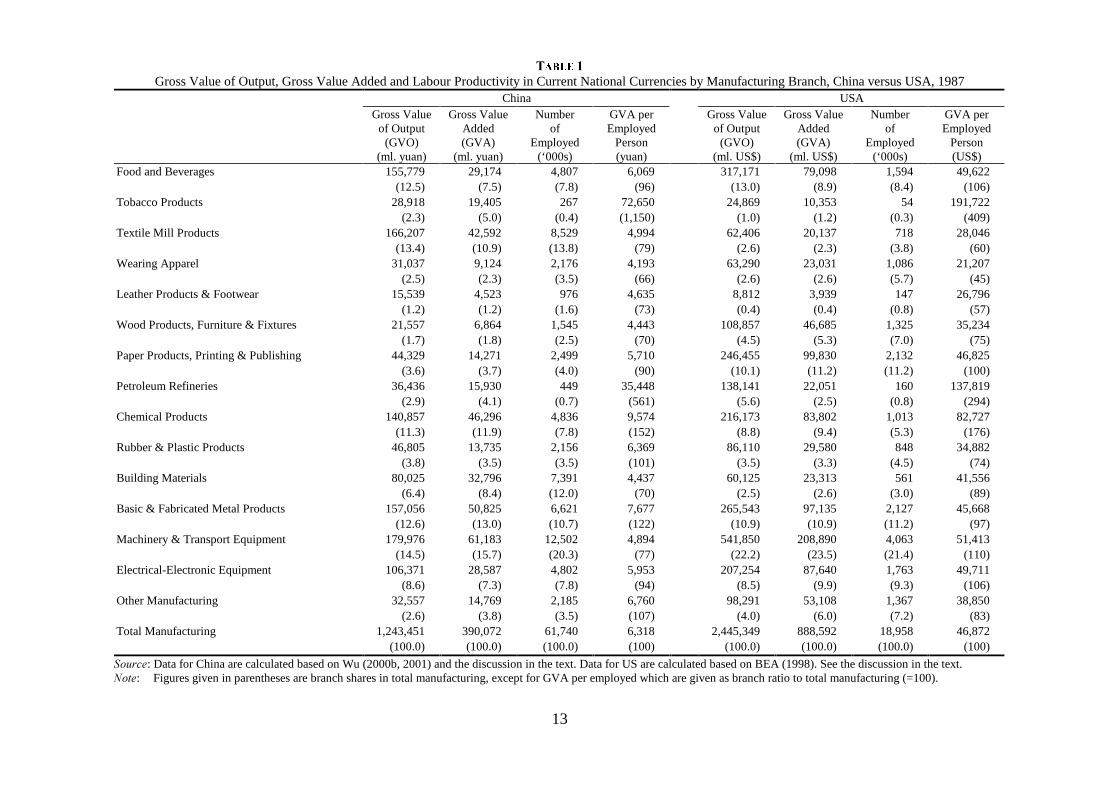
�$%/(��Gross Value of Output, Gross Value Added and Labour Productivity in Current National Currencies by Manufacturing Branch, China versus USA, 1987

China USAGross Value

of Output(GVO)

(ml. yuan)

Gross ValueAdded(GVA)

(ml. yuan)

Numberof

Employed(‘000s)

GVA perEmployed

Person(yuan)

Gross Valueof Output

(GVO)(ml. US$)

Gross ValueAdded(GVA)

(ml. US$)

Numberof

Employed(‘000s)

GVA perEmployed

Person(US$)

Food and Beverages 155,779 29,174 4,807 6,069 317,171 79,098 1,594 49,622(12.5) (7.5) (7.8) (96) (13.0) (8.9) (8.4) (106)

Tobacco Products 28,918 19,405 267 72,650 24,869 10,353 54 191,722(2.3) (5.0) (0.4) (1,150) (1.0) (1.2) (0.3) (409)

Textile Mill Products 166,207 42,592 8,529 4,994 62,406 20,137 718 28,046(13.4) (10.9) (13.8) (79) (2.6) (2.3) (3.8) (60)

Wearing Apparel 31,037 9,124 2,176 4,193 63,290 23,031 1,086 21,207(2.5) (2.3) (3.5) (66) (2.6) (2.6) (5.7) (45)

Leather Products & Footwear 15,539 4,523 976 4,635 8,812 3,939 147 26,796(1.2) (1.2) (1.6) (73) (0.4) (0.4) (0.8) (57)

Wood Products, Furniture & Fixtures 21,557 6,864 1,545 4,443 108,857 46,685 1,325 35,234(1.7) (1.8) (2.5) (70) (4.5) (5.3) (7.0) (75)

Paper Products, Printing & Publishing 44,329 14,271 2,499 5,710 246,455 99,830 2,132 46,825(3.6) (3.7) (4.0) (90) (10.1) (11.2) (11.2) (100)

Petroleum Refineries 36,436 15,930 449 35,448 138,141 22,051 160 137,819(2.9) (4.1) (0.7) (561) (5.6) (2.5) (0.8) (294)

Chemical Products 140,857 46,296 4,836 9,574 216,173 83,802 1,013 82,727(11.3) (11.9) (7.8) (152) (8.8) (9.4) (5.3) (176)

Rubber & Plastic Products 46,805 13,735 2,156 6,369 86,110 29,580 848 34,882(3.8) (3.5) (3.5) (101) (3.5) (3.3) (4.5) (74)

Building Materials 80,025 32,796 7,391 4,437 60,125 23,313 561 41,556(6.4) (8.4) (12.0) (70) (2.5) (2.6) (3.0) (89)

Basic & Fabricated Metal Products 157,056 50,825 6,621 7,677 265,543 97,135 2,127 45,668(12.6) (13.0) (10.7) (122) (10.9) (10.9) (11.2) (97)

Machinery & Transport Equipment 179,976 61,183 12,502 4,894 541,850 208,890 4,063 51,413(14.5) (15.7) (20.3) (77) (22.2) (23.5) (21.4) (110)

Electrical-Electronic Equipment 106,371 28,587 4,802 5,953 207,254 87,640 1,763 49,711(8.6) (7.3) (7.8) (94) (8.5) (9.9) (9.3) (106)

Other Manufacturing 32,557 14,769 2,185 6,760 98,291 53,108 1,367 38,850(2.6) (3.8) (3.5) (107) (4.0) (6.0) (7.2) (83)

Total Manufacturing 1,243,451 390,072 61,740 6,318 2,445,349 888,592 18,958 46,872(100.0) (100.0) (100.0) (100) (100.0) (100.0) (100.0) (100)

������: Data for China are calculated based on Wu (2000b, 2001) and the discussion in the text. Data for US are calculated based on BEA (1998). See the discussion in the text.����: Figures given in parentheses are branch shares in total manufacturing, except for GVA per employed which are given as branch ratio to total manufacturing (=100).

14

.���4&�/���

.�����'�����0�� ��$����� �1� ��� � 2�(GVA)

The basic data on manufacturing GVA for 1952-97 are the BEA annual chained

estimates of Gross Product Originating by industry, which is a new method to replace

the fixed weights to calculate constant price GDP (GVA) indices. An important

property of chain-type quantity indices is that the implied growth rates are not affected

by a shift in the benchmark year and that chain-type indices incorporate the changes in

the industry-composition.16 In this regard, our fixed-weight (1987) Chinese GVA data

are not exactly compatible with the US GVA data. We do not attempt to correct for

this incompatibility because a) it is not important for our purpose in this study and b)

there are no data that allow such correction.

The new BEA GVA data are not available for the period 1952-97. The Groningen

Growth and Development Centre (GGDC) has produced a 1987-based series that

satisfies our needs. The work by GGDC also takes into account the differences

between the 1972 SIC (Standard of Industrial Classification) and the 1987 SIC, and

adjusted the series under the former (1952-86) to the latter (Inklarr and Timmer,

2001). In this study we adopt the GGDC-adjusted series of GVA. The 1987

benchmark figures are given in Table 1. The GGDC-adjusted figures for selected

years are given in Appendix Table A2. The 1987 benchmark branch-level GVO data

are also obtained from BEA (1998) (Table 1).

.�����1� ��� � 2��������� �

The full-time equivalent employment data by branch are originally constructed by

BEA (1998). The only adjustment that needs to be made to this series is the

conversion of the 1972 SIC-based series (1952-86) to the 1987 SIC. We also adopt the

conversion made by GGDC (Inklaar and Timmer, 2001). The GGDC-adjusted figures

for selected years are reported in Appendix Table A2. The 1987 benchmark figures

are reported in Table 1.

16 The downside of chain type indices is that they are not additive, that is, the sum of the parts ofthe aggregate is not equal to the aggregate itself. Normally, the further they are away from thebenchmark year, the bigger is the discrepancy, and typically, the higher is the sum of the componentsrelative to the total the further back in time (Inklaar and Timmer, 2001). However, this problem is not asignificant source of bias in this study.

15

.���(�4 ��0�� ����1����������� ���

Calculation of the unit values of matched products is based on product-specific

gross value of output and quantity of output. They are obtained from the US 1987

Census of Manufactures (US Department of Commerce, 1990).

�$� +����������*���������

5��� ����������678��� �94&����� ��� �����

Following the ICOP PPP estimation steps explained in Section 3, we have

calculated China/US production PPPs for each branch in manufacturing for the

benchmark year 1987 (Table 2). In this exercise 66 product or product-group matches

of 39 sample industries are made. These sample-industry PPPs are then aggregated

into 14 manufacturing branches that have been used in ICOP studies. The PPPs for

Chinese manufacturing as a whole at both Chinese and US weights are the weighted

average of branch PPPs with gross value of output as weights. They are also used as

proxies for the “other manufacturing” branch. The results reported in Table 2 also

include the calculation of Fisher (geometric mean) PPPs.

The matched value of output in this comparison represents 35.7 percent of the

gross value of output in China and 17.2 percent in the USA (see Appendix Table A3),

which is similar to the coverage in Szirmai and Ren (2000) of 37.1 and 18.9 percent,

respectively. This coverage is fairly reasonable given the usual data problems in this

kind of exercise and is in line with similar exercises for the former centrally planned

economies.17

17 For example, the corresponding figures are 18.5 percent and 16.3 percent for a USSR/UScomparison, 32.0 and 23.2 for a Czechoslovakia/West Germany comparison, 33.1 and 19.3 for aHungary/West Germany comparison, and 33.6 and 19.4 for a Poland/West Germany comparison(Kouwenhoven, 1996, Table 5). Even for industrialized market economies, the coverage is not high.For example, a West Germany/US comparison by van Ark and Pilat (1993) manages to cover only 24.4percent of West Germany’s manufacturing output and 24.8 percent of US manufacturing output.

16

%$%/(��Industry-of-Origin PPPs and Price Levels by Major Manufacturing Branch, China/USA, 1987

PPP (Yuan/US$) Relative Price Level

At Chinese

Quantity

weight

At US

Quantity

weight

Geometric

mean

PPP over

Official

Exchange

Rate

PPP over

Market

Exchange

Rate

Food Products 1.92 2.43 2.16 0.58 0.38

Beverages 2.63 1.99 2.29 0.62 0.40

(Food and Beverages) (2.02) (2.35) (2.18) (0.59) (0.38)

Tobacco Products 0.77 0.77 0.77 0.21 0.14

Textile Mill Products 0.57 1.02 0.76 0.21 0.14

Wearing Apparel 1.12 1.12 1.12 0.30 0.20

Leather Products & Footwear 1.95 2.63 2.26 0.61 0.40

Wood Products, Furniture & Fixtures 7.96 7.90 7.93 2.13 1.39

Paper Products, Printing & Publishing 3.59 3.73 3.66 0.98 0.64

Petroleum Refineries 3.27 4.69 3.92 1.05 0.69

Chemical Products 4.78 4.56 4.67 1.26 0.82

Rubber & Plastic Products 0.65 2.28 1.21 0.33 0.21

Building Materials 2.35 1.93 2.13 0.57 0.37

Basic & Fabricated Metal Products 2.89 5.17 3.87 1.04 0.68

Machinery & Transport Equipment 1.95 6.57 3.58 0.96 0.63

Electrical-Electronic Equipment 5.42 5.49 5.45 1.47 0.96

Total Manufacturing 1.97 4.92 3.11 0.84 0.55

Official Exchange Rate 3.72 3.72 3.72 n.a. n.a.

Market Exchange Rate* 5.70 5.70 5.70 n.a. n.a.

&� ���: Author’s estimation. See Section 3 for methodology and Section 4 for the data used.:���: *Referring to China’s foreign exchange “swap market” rate for 1987 (Wu, 1998b). n.a. = Not

applicable.

As shown in Table 2, the average PPP for total manufacturing is 3.11 yuan per

US dollar for 1987 which is lower than but not significantly different from the then

prevailing official (planning-controlled) exchange rate of 3.72 yuan. By contrast,

Szirmai and Ren (2000) estimate a PPP as 1.45 for 1985, which is only 50 percent of

the official exchange rate of 2.90. It may be argued that for a centrally planned

economy the spread between average PPP and official exchange rate should not be so

large as estimated in Szirmai and Ren. This is because exchange rate control has to be,

by its nature, associated with price control, or the level of controlled exchange rate has

to be close to the average production costs that can be reflected by PPP estimates.18 If

18 A study on the Soviet manufacturing by Kouwenhoven (1996, Table 4) also finds that at the1987 benchmark the PPP of ruble (0.455 ruble = US$1) is not significantly different from the official(planning-controlled) exchange rate of ruble (0.523 ruble = US$1).

17

this is true, then Szirmai and Ren may have underestimated the yuan/USD PPP or

overestimated the value of yuan.

Studies on export costs in China may also shed some light on this discussion,

even though the estimation of Chinese export costs does not follow production

approach and hence provides no sector/industry perspective. Lardy (1992) estimates

the average costs of Chinese exports to be 3.67 yuan per US dollar for 1985 and 4.20

for 1987, whereas using a CPI (consumer price index) method Wu (1998) arrives at

4.50 and 5.37, respectively. These estimates could be compared with China’s effective

exchange rates of 3.49 and 4.17, respectively, which are adjusted by the planning and

market shares in foreign exchange transactions. These studies show that official

exchange rate was often forced to adjust to changes in export costs. The depreciation

of yuan in 1985-87, from 2.90 down to 3.72 yuan per US dollar, was an attempt to

make such an adjustment (Wu, 1998, Table 2).

It is not surprising that the average PPP for manufacturing is only 55 percent of

the yuan’s market exchange rate (yuan/USD PPP of 3.11 versus yuan/USD exchange

rate of 5.70), or the yuan’s domestic purchasing power is about 1.8 times its

international purchasing power, because the latter largely reflects the prices of the

tradables, which are mainly on the “market track” under the prevailing dual-track

price system.

5��� *�����������9������������ �������������$��� ��2�

PPP estimates can reflect the relative costs of, and hence comparative advantage

in, manufacturing of the countries being compared. As shown in Table 2, the lowest

PPP is found in Chinese textiles (0.76), followed by tobacco products (0.77) and

wearing apparel (1.12), largely reflecting low costs and comparative advantage of

these products produced in China. For most of the branches with high PPPs (higher

than official exchange rate as given in Table 2) China has obviously no comparative

advantage. They include wood products, for which the highest PPP was found (7.93),

followed by electrical-electronic machinery (5.45), chemical products (4.67),

petroleum refineries (3.92) and basic and fabricated metal products (3.87).

Using US prices as references, China’s relative price levels across manufacturing

branches can be derived by comparing the PPP estimates with Chinese official and

market exchange rates. Reported in the last columns of Table 2, these price levels can

also serve as indicators of China’s relative costs of, and hence comparative advantage

in, individual manufacturing branches.

Another point to address is that the PPPs with US quantity weights are found

higher than the PPPs with Chinese quantity weights. This is similar to the pattern

found by Szirmai and Ren (2000), which is expected in bilateral comparisons between

18

rich and poor countries. Due to differences in both production structure and consumer

preferences, products which are relatively cheap and common in the USA will tend to

be expensive and rare in countries like China and vice versa. Therefore, at least

theoretically, industries with high PPPs (low-value yuan) should receive high quantity

weights in the USA and low weights in China, whereas industries with low PPPs

(high-value yuan) should receive low weights in the US and high weights in China.

There are some good examples to support this theory in our findings. Referring to

Tables 1 and 2, branches with high PPPs or factor costs in China, such as manufacture

of wood and paper, account for larger shares in total manufacturing output in the USA

than in China, whereas branches with low PPPs or factor costs in China, such as

textiles and building materials, account for smaller shares in the USA than in China.

There are, however, some interesting exceptions in our findings. The output share of

wearing apparel and rubber-plastics products seems too low in China if judged by the

��� PPPs of these branches and the output share of metal products and machinery

seems too high if assessed by the �2� PPPs of these branches. This clearly reflects the

structural distortions resulting from the government’s costly industrial strategy under

central planning that focused on heavy industries at the expense of light industries.

5�(� ��������������� ������������� �����������678�"� �����#

Applying the estimated PPPs in Table 2 to Chinese and US gross value added

(GVA) in Table 1, we can examine Chinese and US output level on a comparative

basis, because this approach measures Chinese and US manufacturing outputs using

the same set of prices. Such a PPP-based comparison can to a large extent correct for

the underestimation of Chinese GDP due to price distortions. The derived

comparative GVAs can show the position (scale) of Chinese manufacturing industries

relative to that of the USA.

As reported in Table 3, at the 1987 benchmark, total Chinese manufacturing

output was about 15.9 percent of the US level in GVA.19 The estimates suggest that

the largest manufacturing branch in China in 1987 was textiles which was about 2.8

times the US textiles industry, followed by tobacco (2.4 times), building materials (66

percent), leather-footwear (51 percent), rubber-plastics (38 percent) and wearing

apparel (36 percent), whereas the smallest branch in China was wood products which

was only less than 2 percent of the US level, followed by paper-printing industry (3.9

percent), electrical-electronic equipment (6.0 percent) and machinery (8.2 percent).

19 If measured in gross value of output (GVO), which can be done following the same approachwith the GVO data in Table 1, China’s relative position would be 18.9 percent of the US level, orroughly one fifth of the size of US manufacturing in 1987 (PPP) dollars.

19

Because of the importance of manufacturing for any economy in general and for these

two countries in particular, these findings suggest the strength of the Chinese

economy relative to that of the USA. Undoubtedly, there is still an enormous gap for

the Chinese to fill.

%$%/(�'Gross Value Added (GVA) by Major Manufacturing Branch at 1987 Chinese and US Producer Prices,

and China/USA Comparative Output Level (USA=100)

At Chinese Producer Prices At US Producer Prices Geometric

China

(million

87yuan)

USA

(million

87yuan)

China/

USA

(%)

China

(million

87US$)

USA

(million

87US$)

China/

USA

(%)

mean

China/

USA(%)

Food Products & Beverages 29,174 185,608 15.72 14,436 79,098 18.25 16.94

Tobacco Products 19,405 7,972 243.42 25,201 10,353 243.42 243.42

Textile Mill Products 42,592 20,584 206.91 74,685 20,137 370.89 277.02

Wearing Apparel 9,124 25,683 35.53 8,182 23,031 35.53 35.53

Leather Products & Footwear 4,523 10,360 43.66 2,320 3,939 58.89 50.71

Wood Products, Furniture & Fixtures 6,864 369,013 1.86 863 46,685 1.85 1.85

Paper Products, Printing & Publishing 14,271 372,666 3.83 3,974 99,830 3.98 3.90

Petroleum Refineries 15,930 103,473 15.40 4,875 22,051 22.11 18.45

Chemical Products 46,296 382,011 12.12 9,681 83,802 11.55 11.83

Rubber & Plastic Products 13,735 67,426 20.37 21,281 29,580 71.94 38.28

Building Materials 32,796 45,098 72.72 13,972 23,313 59.93 66.02

Basic & Fabricated Metal Products 50,825 502,267 10.12 17,588 97,135 18.11 13.54

Machinery & Transport Equipment 61,183 1,372,060 4.46 31,301 208,890 14.98 8.17

Electrical-Electronic Equipment 28,587 481,057 5.94 5,274 87,640 6.02 5.98

Other Manufacturing 14,769 261,291 5.65 7,497 53,108 14.12 8.93

Total Manufacturing 390,072 4,206,569 9.27 241,129 888,592 27.14 15.86

&� ���: Derived based on data in Table 1 and the PPP estimates in Table 2.

The same approach can be used to derive comparative labour productivity for

individual manufacturing branches in China. The results are reported in Table 4. At

the 1987 benchmark, Chinese comparative labour productivity in manufacturing was

4.3 percent of the US level (USA=100), which is a Fisher average of 2.7 at Chinese

producer prices and 6.8 at US producer prices. This is lower than the 5.7 percent

estimated by Szirmai and Ren (2000), which could be due to any of the factors or the

combined effect of them discussed in the data section.20

20 This is also lower than 7.9 percent estimated for India (1986) by van Ark (1991), 10 percent forIndonesia (1987) by Szirmai (1994) and 26.4 percent for South Korea (1987) by Pilat (1994). However,since the sector, ownership, size of establishment coverage of these studies vary, these comparisons areonly indicative.

20

%$%/(�)Labour Productivity (GVA per Employed Person) by Major Manufacturing Branch at 1987 Chinese

and US Producer Prices, and China/USA Comparative Labour Productivity Level (USA=100)

At Chinese Producer Prices At US Producer Prices Geometric

China

(87 yuan)

USA

(87 yuan)

China/

USA

(%)

China

(87US$)

USA

(87US$)

China/

USA

(%)

Mean

China/

USA(%)

Food Products & Beverages 6,069 116,442 5.21 3,003 49,622 6.05 5.62

Tobacco Products 72,650 147,626 49.21 94,350 191,722 49.21 49.21

Textile Mill Products 4,994 28,669 17.42 8,757 28,046 31.22 23.32

Wearing Apparel 4,193 23,649 17.73 3,760 21,207 17.73 17.73

Leather Products & Footwear 4,635 70,473 6.58 2,377 26,796 8.87 7.64

Wood Products, Furniture & Fixtures 4,443 278,500 1.60 558 35,234 1.58 1.59

Paper Products, Printing & Publishing 5,710 174,796 3.27 1,590 46,825 3.40 3.33

Petroleum Refineries 35,448 646,708 5.48 10,848 137,819 7.87 6.57

Chemical Products 9,574 377,108 2.54 2,002 82,727 2.42 2.48

Rubber & Plastic Products 6,369 79,511 8.01 9,869 34,882 28.29 15.05

Building Materials 4,437 80,389 5.52 1,890 41,556 4.55 5.01

Basic & Fabricated Metal Products 7,677 236,139 3.25 2,656 45,668 5.82 4.35

Machinery & Transport Equipment 4,894 337,696 1.45 2,504 51,413 4.87 2.66

Electrical-Electronic Equipment 5,953 272,863 2.18 1,098 49,711 2.21 2.20

Other Manufacturing 6,760 191,142 3.54 3,432 38,850 8.83 5.59

Total Manufacturing 6,318 230,608 2.74 3,207 46,872 6.84 4.33

&� ���: Derived based on data in Table 1 and the PPP estimates in Table 2.

In 1987, the manufacturing branches with low comparative labour productivity,

and hence no comparative advantage, were, not so surprisingly, wood products (only

1.6 percent of the US level), machinery-transportation equipment (2.7 percent),

chemical products (2.5) and electrical-electronic equipment (2.2), whereas the

branches with high comparative labour productivity, and hence strong comparative

advantage, were tobacco (49.2), textiles (23.3), wearing apparel (17.7) and rubber-

plastics (15.1). Compared with the findings in Tables 2 and 3, these suggest that in

most cases, the manufacturing branches (such as tobacco, textiles, wearing apparel,

rubber-plastics) that have lower PPPs tend to enjoy higher comparative labour

productivity and larger share in output, which is in line with the theory. We shall

further examine this in a dynamic perspective.

5�. ��������������� ������������� ��� ������� 2�*

Following exactly the techniques used in deriving the 1987-benchmark output

and labour productivity, estimates for 1952-97 are obtained using the time series of

output and labour input introduced in Section 4. The estimates for the comparative

output (GVA) level of Chinese manufacturing are reported in Table 5 and the

estimates for the comparative labour productivity level of Chinese manufacturing are

reported in Table 6. Readers are reminded to closely follow the concept of “China-US

21

comparative level” in the discussion below to avoid being overwhelmed by the

common sense of “growth” in a dynamic perspective. For example, a decline in

Chinese comparative output or labour productivity over a certain period is a decline in

������� rather than ����� �� terms. It declines because it grows not as fast as that of

the USA or it declines more rapidly than that of the USA. The same should be applied

to an increase in comparative output and productivity. Chinese electronic industry

(grouped with electrical equipment in this study) is a good example. Its labour

productivity in ����� �� terms grew at 16.6 percent a year in 1987-97, one of the fast

growing industries, but in ������� terms it only grew at 2.8 percent a year, which

means that its growth was only 2.8 percentage points faster than that of the US

counterpart (see Appendix Table A4).

Over the entire period 1952-97, as shown in Table 5, the comparative output

level of Chinese manufacturing (the USA=100) increased from 2.9 to 27.8, up by 5.1

percent per annum, with an increase by 4.7 percent per annum for the pre-reform

period 1952-78 and an increase by 5.7 percent per annum for the post-reform period

1978-97. During the central planning period the branches that grew fastest were

metals, machinery and electrical-electronic equipment, while during the reform period

wearing apparel, leather and footwear, tobacco, building materials and food grew

fastest. These findings generally reflect the policy orientation of the two periods, that

is, heavy industry-oriented industrialisation under central planning and light industry-

oriented development during economic reform.

In terms of the relative size (with the USA=100) of branches, in 1977 (the time

representing the pre-reform level) there was only one branch that was larger than the

US counterpart, that is, textiles with a size of 1.7 times the US size. By 1997, there

were 6 branches that were either greater or similar to the US level. They are, by the

relative size, textiles (450), tobacco (445), leather-footwear (319), wearing apparel

(214), building materials (128) and rubber-plastics (93) which are all labour-intensive

indeed. On the other hand, branches at about or below 20 percent of the US level are

wood (5), paper-printing (10), electrical-electronic (10), machinery (14) and metals

(22) which rely more on either natural resources or capital and technology.

By far, the findings seem to well conform to the theory of comparative advantage.

However, we are not so sure until we know whether the performance of comparative

labour productivity in Chinese manufacturing can show a clear sign of catch up

(falling behind) of the branches that grew faster (slower) during the economic reform.

22

�$%/(��Comparative Performance of Chinese and US Manufacturing: Gross Value Added in 1987 PPPs by Major Manufacturing Branch, China versus USA, 1952-1997

(Fisher Average, USA=100)

TotalManufac-

turing

Food andBeverages

TobaccoProducts

TextileMill

Products

WearingApparel

Leather,Footwear

WoodProducts

Paper,Printing

PetroleumRefineries

Chemicals Rubber,Plastics

BuildingMaterials

MetalProducts

Machinery-TransportEquipment

Electrical-ElectronicEquipment

Others

1952 2.93 2.34 15.23 155.74 8.56 2.23 1.58 0.36 4.54 1.58 3.13 4.55 0.41 0.30 0.27 3.161953 3.53 2.71 22.13 198.20 10.37 2.63 2.32 0.40 4.82 1.82 3.89 5.46 0.49 0.48 0.44 4.971954 4.22 2.93 24.79 229.47 12.32 3.85 2.76 0.47 5.35 2.47 5.44 6.94 0.74 0.61 0.49 4.271955 3.73 3.17 22.31 194.13 9.57 3.51 2.13 0.48 5.36 2.40 4.99 7.40 0.79 0.65 0.44 2.841956 4.70 3.28 23.03 233.63 12.39 4.29 2.79 0.59 5.77 2.90 5.84 8.76 1.15 1.22 0.67 4.151957 4.97 3.53 25.25 227.45 11.00 5.51 2.72 0.75 6.58 3.28 7.19 11.30 1.49 1.42 1.22 5.021958 7.97 4.84 25.21 298.11 14.37 6.46 4.29 1.01 7.15 4.42 12.11 10.28 2.94 5.24 4.02 6.731959 9.07 5.78 27.50 322.53 15.80 6.52 4.49 1.29 7.03 5.31 9.94 10.97 4.19 5.85 5.88 9.681960 8.94 4.25 21.75 245.04 11.01 7.92 5.23 1.35 7.57 6.02 10.56 13.32 5.50 7.22 6.66 11.581961 4.52 2.61 11.83 134.56 6.43 4.87 2.62 0.81 8.10 3.08 7.17 8.95 3.03 2.23 2.13 5.841962 3.54 2.67 10.96 102.78 7.16 3.42 2.20 0.79 8.33 2.97 7.91 8.97 2.27 0.98 1.18 4.741963 3.90 2.78 14.40 104.41 7.48 3.64 2.32 0.85 8.95 3.53 8.69 9.38 2.38 0.98 0.97 5.161964 4.62 3.77 19.15 136.07 8.68 3.33 2.55 0.88 9.67 4.17 9.70 10.29 2.54 1.27 0.98 5.891965 5.30 4.21 22.38 163.49 9.91 3.20 2.48 1.02 10.19 5.04 10.48 11.04 2.91 1.55 1.01 7.031966 5.83 4.35 24.89 173.61 10.50 4.33 2.39 1.16 11.08 6.01 10.96 11.93 3.31 1.87 1.47 8.251967 4.91 4.11 21.83 158.03 9.93 5.32 2.46 1.09 12.31 4.61 9.79 9.54 2.24 1.15 1.12 7.591968 4.39 3.94 22.90 147.20 7.54 5.23 1.84 0.93 13.26 3.45 8.43 8.29 1.95 1.10 0.83 6.291969 5.66 3.67 29.21 187.05 8.21 6.24 2.03 1.08 15.35 4.77 10.66 10.45 2.84 1.79 1.55 7.181970 7.52 4.15 31.85 198.95 9.10 9.17 2.31 1.27 14.77 5.71 15.63 13.92 4.26 3.66 3.00 8.101971 7.92 4.37 27.85 183.67 10.17 9.67 2.24 1.35 15.49 6.22 15.07 16.18 5.30 4.64 3.46 7.631972 7.61 4.66 28.83 166.22 10.20 10.19 2.02 1.35 17.69 6.28 14.66 15.97 5.21 4.53 3.27 7.401973 7.51 4.83 31.37 177.89 10.64 10.57 1.67 1.37 18.64 6.13 14.78 15.10 4.85 4.63 3.16 8.251974 7.73 6.00 31.98 189.64 11.70 10.67 1.75 1.37 21.75 6.30 15.66 15.96 4.33 4.81 3.70 8.371975 9.69 6.13 35.12 231.11 13.99 12.79 2.03 1.66 24.26 7.26 20.50 21.30 6.08 6.51 4.32 9.601976 8.50 5.67 34.86 181.42 13.87 11.84 1.69 1.53 24.97 5.98 19.80 19.32 4.95 5.55 3.72 8.661977 8.93 6.51 44.72 170.77 13.38 14.11 1.82 1.59 25.01 6.47 19.53 22.13 5.40 5.53 3.24 8.451978 9.72 6.67 41.39 184.71 11.61 15.21 1.74 1.78 37.65 7.75 21.75 24.50 6.83 6.07 3.81 8.561979 10.21 7.12 45.96 190.45 12.66 19.36 2.04 1.91 28.42 8.57 22.81 26.62 7.37 6.10 3.83 8.50

23

�$%/(���(Continued)

TotalManufac-

turing

Food &Beverages

TobaccoProducts

TextileMill

Products

WearingApparel

Leather,Footwear

WoodProducts

Paper,Printing

PetroleumRefineries

Chemicals Rubber,Plastics

BuildingMaterials

MetalProducts

Machinery-TransportEquipment

Electrical-ElectronicEquipment

Others

1980 11.31 7.38 56.44 213.03 16.39 24.45 2.24 2.19 35.54 10.41 25.73 32.57 7.70 6.05 3.44 9.061981 11.15 9.25 58.99 229.08 17.74 29.24 2.25 2.20 20.00 9.98 22.53 36.78 7.04 5.32 3.00 8.881982 12.74 9.50 79.72 252.65 18.67 27.43 2.48 2.39 24.17 10.54 27.55 50.38 9.61 6.44 3.15 9.001983 12.93 10.15 105.24 220.85 17.20 27.76 2.23 2.55 19.28 9.96 30.78 47.67 11.25 7.18 3.63 8.711984 12.78 12.22 124.50 218.24 18.05 30.97 2.12 2.79 18.41 10.76 31.88 47.83 10.66 7.32 3.99 7.831985 14.16 13.75 146.45 248.14 20.66 37.47 2.08 3.26 16.78 12.26 34.79 53.54 11.57 8.17 5.57 7.971986 15.60 16.18 191.22 265.42 42.80 50.01 1.92 3.54 27.07 12.07 37.62 58.02 12.81 7.78 5.28 8.971987 15.86 16.94 243.42 277.02 35.53 50.71 1.85 3.90 18.45 11.83 38.28 66.02 13.54 8.17 5.98 8.931988 16.64 18.28 280.20 303.45 42.86 51.86 1.89 4.20 18.59 12.92 41.86 73.34 13.43 8.97 6.69 8.121989 16.92 19.43 350.39 313.85 43.61 51.39 1.83 4.44 15.63 13.39 40.40 71.56 14.37 8.39 6.27 8.661990 16.84 17.53 433.79 280.99 47.32 60.36 1.81 4.68 27.61 13.32 42.40 70.72 15.64 7.52 5.90 8.571991 19.35 19.98 534.39 301.83 54.72 71.48 1.88 5.15 34.81 14.70 49.17 89.83 17.94 9.52 6.61 9.481992 21.86 22.87 653.85 290.26 62.54 94.84 2.04 5.99 37.02 15.90 55.72 94.61 19.85 11.93 7.91 11.181993 24.24 24.77 693.64 306.60 93.93 144.37 2.65 6.62 41.04 17.58 63.63 113.22 21.01 12.92 9.14 14.971994 26.25 25.37 473.18 311.75 113.54 182.19 2.60 7.26 37.72 17.33 75.45 117.39 20.77 15.19 13.65 14.911995 31.80 26.44 423.69 433.84 261.21 336.43 7.70 10.46 33.89 22.06 82.61 134.07 20.98 20.29 11.92 20.591996 28.71 28.45 437.23 393.76 191.05 328.99 4.78 9.59 33.01 21.12 100.84 136.93 21.20 18.00 9.44 18.111997 27.80 29.43 444.67 450.39 213.99 319.26 5.02 9.91 42.03 22.84 93.02 128.28 21.71 14.20 10.01 19.76

1952-57 11.15 8.56 10.65 7.87 5.14 19.82 11.48 15.47 7.71 15.74 18.11 19.96 29.46 36.88 35.03 9.681958-62 -6.53 -5.44 -15.37 -14.69 -8.24 -9.09 -4.19 1.12 4.82 -1.96 1.91 -4.51 8.83 -7.16 -0.63 -1.151963-65 14.34 16.42 26.86 16.74 11.47 -2.19 4.12 8.83 6.97 19.34 9.84 7.14 8.62 16.33 -4.87 14.021966-70 7.26 -0.27 7.31 4.00 -1.70 23.41 -1.42 4.53 7.71 2.51 8.32 4.76 7.92 18.79 24.25 2.871971-78 3.27 6.12 3.33 -0.92 3.09 6.54 -3.48 4.29 12.40 3.89 4.21 7.32 6.08 6.55 3.03 0.701979-87 5.59 10.90 21.76 4.61 13.23 14.31 0.70 9.15 -7.62 4.81 6.49 11.64 7.89 3.35 5.13 0.471988-97 5.77 5.68 6.21 4.98 19.67 20.20 10.48 9.77 8.58 6.80 9.28 6.87 4.84 5.68 5.28 8.26

1952-78 4.72 4.12 3.92 0.66 1.18 7.66 0.37 6.30 8.48 6.31 7.74 6.69 11.44 12.32 10.71 3.901979-97 5.68 8.12 13.31 4.80 16.57 17.37 5.73 9.47 0.58 5.85 7.95 9.10 6.27 4.57 5.21 4.50

1952-97 5.13 5.79 7.79 2.39 7.41 11.66 2.60 7.63 5.07 6.12 7.83 7.70 9.23 8.98 8.35 4.15

������: Derived based on PPP estimates in Table 2 and the basic time series data for China and the USA as explained in Section 4.

24

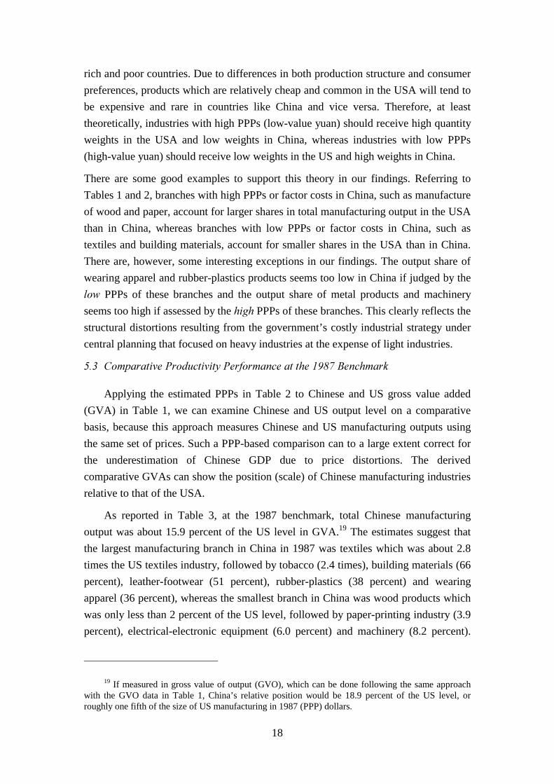
�$%/(��Comparative Performance of Chinese Manufacturing: Gross Value Added per Employed Person in 1987 PPPs by Major Manufacturing Branch, China versus USA,

1952-1997, (Fisher Average, USA=100)

TotalManufac-

turing

Food andBeverages

TobaccoProducts

TextileMill

Products

WearingApparel

Leather,Footwear

WoodProducts

Paper,Printing

PetroleumRefineries

Chemicals Rubber,Plastics

BuildingMaterials

MetalProducts

Machinery-TransportEquipment

Electrical-ElectronicEquipment

Others

1952 3.04 6.54 31.23 93.22 7.96 4.93 0.90 1.25 56.07 6.40 35.35 4.43 0.78 1.45 2.53 1.651953 3.56 6.63 36.54 110.45 9.20 5.35 1.22 1.30 43.39 6.39 37.91 4.69 0.92 2.18 3.95 2.521954 3.60 6.17 37.31 106.29 9.05 6.70 1.15 1.34 40.19 8.32 48.06 5.43 1.11 2.34 3.76 1.941955 3.59 4.18 31.29 107.55 10.43 7.91 0.95 1.41 39.53 8.32 47.72 4.83 1.59 2.61 3.54 1.561956 4.81 4.66 30.06 123.30 16.28 10.18 1.51 1.78 34.94 7.37 39.31 5.07 2.39 3.66 4.18 2.731957 5.18 4.93 29.30 115.03 14.35 12.80 1.38 2.16 47.72 7.96 45.45 7.03 2.93 4.03 7.16 3.371958 3.44 3.19 22.22 96.55 16.32 9.60 3.40 1.44 19.64 1.74 21.41 1.51 0.89 4.15 7.93 3.191959 5.09 4.24 20.25 113.19 23.82 11.90 4.36 2.07 14.50 2.45 20.04 2.14 1.98 5.22 13.24 5.631960 5.31 3.35 26.00 90.26 17.57 13.51 4.89 2.61 15.45 2.99 22.96 2.90 2.40 5.62 13.68 5.611961 3.45 2.57 14.75 57.15 9.55 8.30 1.74 1.88 19.63 2.56 16.48 2.83 2.23 2.15 5.47 4.381962 3.72 3.08 15.98 54.89 13.99 7.78 1.83 2.34 20.05 3.17 22.22 4.41 2.78 1.32 4.26 4.561963 4.15 3.69 23.07 53.53 12.28 7.23 1.37 2.45 23.65 5.31 24.91 5.75 3.62 1.47 3.58 4.151964 4.66 4.80 30.10 62.51 14.24 6.85 1.49 2.53 23.88 5.98 28.37 5.94 3.96 1.88 3.42 4.191965 5.21 5.03 34.07 74.58 17.53 7.13 1.65 3.01 22.68 6.11 32.28 5.37 4.25 2.23 3.43 4.751966 5.70 4.99 35.93 78.99 17.69 9.53 1.51 3.41 24.09 6.92 35.96 5.39 4.74 2.76 5.34 5.291967 4.68 4.88 31.45 72.74 18.27 11.45 1.70 3.28 25.02 5.15 29.21 3.67 3.20 1.53 3.86 4.841968 4.08 4.77 31.67 69.53 15.03 11.80 1.40 2.84 26.12 3.64 26.50 3.11 2.71 1.39 2.59 3.851969 4.74 4.18 38.15 81.97 15.17 12.03 1.49 2.98 29.56 4.53 31.25 3.24 3.65 1.98 4.26 3.771970 5.32 4.32 36.57 77.77 16.31 14.15 1.68 3.13 23.81 4.09 38.98 3.88 4.36 2.98 5.35 3.551971 4.81 3.93 26.22 64.18 16.26 12.36 1.53 2.78 20.14 3.52 30.75 3.71 4.33 2.79 4.43 3.501972 4.48 3.95 26.18 58.26 16.77 11.92 1.52 2.64 18.44 3.21 27.49 3.26 4.14 2.52 3.85 3.411973 4.40 3.89 28.21 61.85 17.06 11.42 1.29 2.62 19.04 2.99 26.43 2.87 4.05 2.63 3.89 3.851974 4.31 4.52 27.06 61.42 17.82 10.13 1.35 2.47 21.36 2.85 24.76 2.69 3.54 2.63 4.41 3.881975 4.52 4.28 25.31 60.76 21.21 9.94 1.60 2.66 21.79 2.91 23.03 2.81 4.23 2.86 3.99 4.101976 3.77 3.80 23.09 49.48 23.16 9.16 1.62 2.35 20.30 2.25 21.58 2.34 3.39 2.31 3.37 2.741977 4.05 4.26 27.20 44.67 24.00 10.41 2.20 2.45 19.95 2.32 21.39 2.56 3.77 2.27 2.95 3.691978 4.51 4.51 24.74 47.93 25.71 10.86 3.98 2.78 29.29 2.73 22.45 2.64 5.03 2.46 3.59 3.741979 4.68 4.12 26.41 43.47 20.35 11.47 2.90 2.81 22.89 3.11 21.29 2.90 5.37 2.80 3.76 3.41

25

�$%/(���(Continued)

TotalManufac-

turing

Food &Beverages

TobaccoProducts

TextileMill

Products

WearingApparel

Leather,Footwear

WoodProducts

Paper,Printing

PetroleumRefineries

Chemicals Rubber,Plastics

BuildingMaterials

MetalProducts

Machinery-TransportEquipment

Electrical-ElectronicEquipment

Others

1980 4.70 4.52 28.07 37.05 14.92 9.53 2.48 2.49 23.97 3.37 14.19 4.53 4.23 2.59 2.19 7.021981 4.51 5.54 29.35 38.12 15.70 11.57 2.38 2.50 13.76 3.19 12.55 4.87 3.75 2.25 1.89 6.931982 4.27 4.34 26.14 30.20 12.06 8.53 2.04 2.42 14.77 3.01 11.93 4.97 4.25 2.46 1.75 6.041983 4.26 4.46 32.87 26.14 11.03 7.90 1.94 2.60 11.22 2.70 13.46 4.63 4.61 2.55 1.99 5.611984 4.24 5.00 35.25 24.37 11.19 7.52 1.85 2.76 9.64 2.73 14.41 4.59 4.33 2.65 2.24 4.851985 4.34 4.93 37.55 23.70 10.83 7.25 1.72 3.06 7.95 2.96 14.47 4.54 4.35 2.88 2.85 4.511986 4.30 5.59 43.30 22.81 21.90 7.86 1.62 3.06 10.34 2.60 14.60 4.33 4.28 2.59 2.43 4.201987 4.33 5.62 49.21 23.32 17.73 7.64 1.59 3.33 6.57 2.48 15.05 5.01 4.35 2.66 2.62 4.131988 4.52 5.89 53.22 24.38 21.22 7.74 1.67 3.60 5.83 2.63 15.85 5.64 4.28 2.90 2.84 3.861989 4.58 6.35 60.80 24.46 21.51 7.65 1.63 3.86 4.54 2.68 15.62 5.70 4.56 2.77 2.63 4.111990 4.46 5.71 73.25 20.91 21.42 8.04 1.56 4.01 7.82 2.57 15.91 5.72 4.83 2.42 2.30 3.821991 4.77 6.37 82.64 20.79 22.48 7.97 1.50 4.15 8.51 2.69 17.06 6.62 5.18 2.83 2.30 3.941992 5.27 7.18 96.03 20.59 25.08 10.10 1.69 4.63 8.55 2.81 19.32 6.81 5.43 3.47 2.59 4.131993 5.73 7.21 92.96 22.77 35.94 13.54 2.25 5.09 11.44 2.83 23.30 7.82 5.31 3.65 2.82 5.581994 6.40 7.47 65.68 23.57 42.00 14.66 2.26 5.61 9.85 2.71 29.09 7.95 5.50 4.48 4.06 5.501995 7.70 7.75 52.85 32.67 90.83 24.03 6.73 7.99 6.06 3.44 30.73 9.14 5.66 6.20 3.19 8.531996 7.20 8.88 56.65 30.71 64.42 23.95 4.44 7.18 5.95 3.30 38.62 9.89 6.00 5.52 3.12 6.271997 7.59 9.27 57.41 38.24 72.84 20.71 4.99 8.27 7.31 3.64 37.08 9.75 6.61 4.70 3.44 9.63

1952-57 11.20 -5.50 -1.27 4.29 12.50 21.04 8.93 11.61 -3.18 4.48 5.15 9.69 30.40 22.72 23.11 15.341958-62 -6.38 -9.00 -11.42 -13.76 -0.50 -9.47 5.77 1.64 -15.92 -16.83 -13.33 -8.93 -1.04 -19.97 -9.84 6.221963-65 11.86 17.76 28.71 10.76 7.81 -2.90 -3.35 8.74 4.19 24.43 13.26 6.83 15.21 19.03 -7.00 1.361966-70 0.41 -2.98 1.43 0.84 -1.43 14.71 0.34 0.79 0.98 -7.69 3.84 -6.30 0.48 5.95 9.30 -5.641971-78 -2.05 0.53 -4.77 -5.87 5.85 -3.26 11.38 -1.49 2.62 -4.95 -6.66 -4.68 1.80 -2.39 -4.87 0.651979-87 -0.45 2.47 7.94 -7.69 -4.04 -3.83 -9.69 2.04 -15.30 -1.05 -4.34 7.36 -1.60 0.87 -3.44 1.101988-97 5.77 5.14 1.55 5.07 15.18 10.49 12.11 9.53 1.08 3.91 9.43 6.88 4.28 5.88 2.77 8.84

1952-78 1.52 -1.42 -0.89 -2.53 4.61 3.09 5.88 3.13 -2.47 -3.23 -1.73 -1.96 7.44 2.05 1.35 3.191979-97 2.78 3.87 4.53 -1.18 5.63 3.46 1.20 5.91 -7.04 1.53 2.68 7.11 1.45 3.48 -0.22 5.10

1952-97 2.05 0.78 1.36 -1.96 5.04 3.24 3.87 4.29 -4.43 -1.25 0.11 1.77 4.87 2.65 0.69 4.00

������: Derived based on PPP estimates in Table 2 and the basic time series data for China and the USA as explained in Section 4.

26

It may be argued that in a more market-oriented and less distorted economy, more

capital will go to the industries that have some comparative advantage, which will

lead to more rapid increase in marginal productivity of labour of these industries. If

this is the case for the post-reform China, in terms of China-US comparison the

industries in which China has comparative advantage should have enjoyed some

degree of catch up, ����������� �.

For the manufacturing as a whole in 1952-97 China’s comparative labour

productivity level rose from about 3.0 to 7.6 (USA=100), up by about 2.1 percent a

year. Dividing the time into two periods, the increase was estimated at 1.5 percent per

annum during the central planning period and 2.8 percent per annum during the

reform period (Table 6). While our findings have shown a clear productivity catch-up

in Chinese manufacturing in 1952-97, they have also suggested a long stagnation at

around 4.5 between 1958 and 1990. The results cannot rule out the possibility

suggested by the Szirmai-Ren study (2000) that there was no catch up in Chinese

manufacturing between the early 1980s and the early 1990s.

�,*85(��Comparative Performance of Chinese Manufacturing: GVA and GVA per Labourer

in 1987 PPPs, 1952-1997(USA=100)

&� ���: Based on Tables 5 and 6.

As depicted in Figure 1, from the early 1950s to the mid 1960s the growth of the

comparative output level was accompanied by the growth of the comparative labour

productivity level in Chinese manufacturing, except for the Great Leap Forward

campaign around 1958-59. But after the mid 1960s, the latter slowed down and was

0

5

10

15

20

25

30

35

1952

1955

1958

1961

1964

1967

1970

1973

1976

1979

1982

1985

1988

1991

1994

1997

Com

para

tive

Out

put/

Prod

ucti

vity

(U

S=10

0) GVA per labourer

GVA

27

eventually left far behind by the former. This suggests that the output growth in

Chinese manufacturing in the 1970s and the 1980s was fuelled mainly by the increase

in labour and physical capital inputs rather than technological progress and efficiency

improvement.

A closer examination of the comparative productivity level of Chinese

manufacturing may raise questions about the radical fluctuations of many branches

over the entire period under study. Such fluctuations could be most explained by

abrupt changes in institutions and development policies in the Chinese economy. To

help understand how these changes might have affected China’s position relative to

that of the USA in manufacturing, in both Tables 5 and 6 we provide the growth rates

of both China’s comparative output and labour productivity in different periods,21

even though most of our discussions will focus on a broader division of pre- and post-

reform periods.

When examining the fluctuations of China’s comparative productivity estimates

in Table 6 it is also important to bear in mind the nature of China’s socialist labour

employment system that prevailed under central planning and still to a large extent

remain in the state sector after the reform. Under this employment system, jobs were

allocated through planning authorities rather than the market. Once a job was assigned

to a person it meant a (working) life-time employment thought it was generally not

changeable. Therefore, if no proper capacity adjustment for labour (or for capital as it

could provide some implication for labour capacity in use), the estimated (����� ��22)

labour productivity could be upward biased if production operation moved from low

to high capacity,23 and downward biased if the opposite happened, other things being

equal.

Comparing the pre- and post-reform periods, the best performer in catch up was

building materials, whose annual growth of comparative productivity rose from -2.0 to

7.1 percent over the two periods. This was followed by wearing apparel (4.6 to 5.6),

21 They are, namely, 1) the first five-year plan period (1952-57) when central planning system andheavy industrialisation strategy were adopted, 2) the Great Leap Forward campaign and its aftermath(1958-62) when the Maoists attempted to boost both agricultural and industrial output by masscampaigns but failed, 3) the post-GLF recovery and adjustment period (1963-65) when light industrieswere paid some attention, 4) the chaotic period of the Cultural Revolution (1966-70), 5) the period of“grasping revolution, promoting production” (1971-78) when both heavy industrialisation and ruralindustrial development were promoted, 6) the early reform period (1979-87) when an export-orienteddevelopment policy was adopted and 7) the period of deepening reform and matketisation (1988-97).

22 The ���������� labour productivity is calculated based on the ����� �� labour productivity ofthe countries being compared and their respective PPPs.

23 It should be noted that in some special cases such as during the Korean War (1951-53) and theGreat Leap Forward (1958-59), workers had to work over their full capacity, that is, 8 hours a day or 48hours a week.

28

tobacco (-0.9 to 4.5) and food (-1.4 to 3.9). Over the two periods, the worst performer

was metals (down from 7.4 to 1.5), followed by wood (down from 5.8 to 1.2),

petroleum (-2.5 to -7.0) and electrical-electronic (1.4 to -0.2) (Table 6). There are,

however, some interesting cases. For example, textiles experienced a process of

falling behind (-2.5 to -1.2), while leather-footwear maintained steady catch up over

the two periods (3.1 to 3.5) (Table 6).

As a result, by 1997 wearing had apparel enjoyed the highest level of

comparative labour productivity (73 percent of the US level), followed by tobacco

(57), textiles (38) and rubber-plastics (37). The electrical-electronic equipment branch

had the lowest level of comparative labour productivity (only 3.4), followed by

chemicals (3.6), machinery (4.7), wood (5.0) and metals (6.6) (Table 6).

The case of textiles may deserve some special attention. Tables 5 and 6 show that

in the 1950s textiles was the largest branch in Chinese manufacturing with a size that

was about 1.6 times that of the USA and a labour productivity that was between a

level similar to and 1.1-1.2 times that of the USA. Is this labour productivity level

plausible for Chinese textiles? Apart from the possible upward bias in the estimates

that are perhaps caused by the lack of labour capacity adjustment as discussed above,

one has to admit that Chinese textile industry should be quite close to its western

counterparts prior to China’s implementation of central planning in the 1950s. Firstly,

China traditionally had strong comparative advantage in textiles which explained why

this industry became the first and, at that time, perhaps the most modernised industry

through foreign trade and investment.24 Secondly, the nature of textile production did

not require heavy investment in technology and human knowledge in which the USA

enjoyed some comparative advantage over China. We could argue that as Table 6

shows, it was the ill-suited central planning system and heavy industry-oriented

government policy that made China fall behind in the industries that China used to

enjoy comparative advantage.

While China’s relatively large size in textiles has maintained for long and even

expanded since the 1980s, its labour productivity has been declining over time. One

possible reason is that prior to the reform textiles in China did not face any

competition while after the reform it only carried on producing low quality products

using the abundant supply of cheap labour. This has made this industry incapable of

adjusting to rapidly changing technologies in textile production that has been driven

by increasingly fierce competition in the world textiles and fashion markets.

24 In fact, it mainly concentrated in China’s coastal cities especially the old treaty ports suchShanghai, Tianjin and Qingdao.

29

Our findings, except for textiles, are quite compatible with the factor cost level

across branches that are suggested by the PPP estimates (Table 2). As we argued

above, China’s market-oriented reform has driven those branches with comparative

advantage to grow faster than those without comparative advantage.

The branch level examination further confirms that China’s catch up since the

1990s is a healthy sign as it happened at the time when the industries in which China

has comparative advantage began to enjoy faster growth, the non-state sector started to

play more important roles in industrial production, and market competition further

intensified.

��� ��� �����������

This study joins the debate of whether Chinese manufacturing has experienced a

significant catch-up with or a process of falling behind the world’s advanced

economies. It has estimated a new set of industry-of-origin China-US PPPs for major

manufacturing industries at 1987 prices. Then using a newly constructed data set, we

have derived China’s comparative labour productivity level in manufacturing for

1952-97.

Firstly, our findings show a clear productivity catch-up in Chinese manufacturing

in 1952-97, but they have also suggested a long stagnation at around 4.5 between 1958

and 1990. Therefore the results cannot rule out the possibility suggested by the

Szirmai-Ren study (2000) that there was no catch up in Chinese manufacturing

especially during the first decade of the reform.

Secondly, since a clear catch up appeared at the time when the market-oriented

reform deepened and market competition intensified, our findings strongly supports

the conditional catch up hypothesis that the changes made China more capable of

improving economic efficiency as well as adopting new technology (Abramovitz,

1989).

Thirdly, the approach used in this study also helps reassess China’s development

policies during the central planning and reform periods because the production PPPs

could serve as an indicator of factor costs in the countries being compared and hence

the degree of distortion in production structure (resource allocation). Our findings

suggest a clear resource misallocation effect under central planning and a somewhat

healthy shift towards Chinese comparative advantage since the market-oriented

reform.

Lastly, our findings show that industries with comparative advantage have been

the engine of the post-reform growth and catch up. This looks encouraging for China

30

at this time when it is facing a historical opening to international competition that will

follow its WTO entry. It is reasonable to expect that if this catch up continues, more

capital with embodied new technologies would be invested to these industries, which

will lead to further catch-up.

���������

Abramovitz, M., 1986. Catching up, forging ahead, and falling behind. Journal ofEconomic History 46, 385-406.

Abramovitz, M., 1989. Thinking About Growth. Cambridge University Press,Cambridge.

BEA (Bureau of Economic Analysis, US Department of Commerce), 1998.<http://www.bea.doc.gov>.

DITS (Department of Industry and Transportation Statistics, SSB), various years.China Industrial Economic Statistical Yearbook. China Statistical PublishingHouse, Beijing.

Gilbert, M. and Associates, 1958. Comparative National Products and Price Levels.OECD, Paris.

Gilbert, M., Kravis, I.B., 1954. An International Comparison of National Products andthe Purchasing Power of Currencies. OEEC, Paris.

Inklarr, R., Timmer, M.P., 2001. Documentation for the US Manufacturing Trend.Groningen Growth and Development Centre, Groningen. Mimeo.

Kouwenhoven, R., 1996. A comparison of Soviet and US industrial performance,1928-90. Paper for The 24th General Conference of the InternationalAssociation of Research in Income and Wealth, Lillehammer, Norway.

Kravis, I.B., 1976. A survey of international comparisons of productivity. TheEconomic Journal 86, 1-44.

Kravis, I.B., 1981. An approximation of the relative real per capita GDP of thePeople’s Republic of China. Journal of Comparative Economics 5, 60-78.

Kravis, I.B., 1984. Comparative studies of national incomes and prices. Journal ofEconomic Literature 22, 1-39.

Kravis, I.B., Heston, A., Summers, R., 1978. International Comparisons of RealProduct and Purchasing Power. The John Hopkins University Press,Baltimore.

Kravis, I.B., Heston, A., Summers, R., 1982. World Product and Income: InternationalComparison of Real Gross Product. The John Hopkins University Press,Baltimore.

Lardy, N.R., 1992. Foreign Trade and Economic Reforms in China, 1978-91.Cambridge University Press, Cambridge, New York.

Maddison, A., van Ark, B., 1988. Comparisons of real output in manufacturing,policy, planning, and research working papers. International EconomicsDepartment, The World Bank, Washington, D.C.

31

Maddison, A., van Ark, Bart, 1994. The international comparison of real product andproductivity. Paper for the 23rd General Conference of the InternationalAssociation for Research in Income and Wealth, St. Andrews, NewBrunswick, Canada, August 21-27.

Maddison, A., 1970. Economic Progress and Policy in Developing Countries. Allen &Unwin, London.

Maddison, A., 1995. Monitoring the World Economy 1820-1992. OECDDevelopment Centre, Paris.

Maddison, A., 1998. Chinese Economic Performance in the Long Run. OECDDevelopment Centre, Paris.

Paige, D., Bombach, G., 1959. A Comparison of National Output and Productivity ofthe United Kingdom and United States. OEEC, Paris.

Pilat, D., 1994. The Economics of Rapid Growth: The Experience of Japan andKorea. Edward Elgar, Aldershot.

Ren, R., 1997. China’s Economic Performance in an International Perspective. OECDDevelopment Centre, Paris.

Ren, R., Chen K., 1994. An expenditure-based bilateral comparison of gross domesticproduct between China and the United States. Review of Income and Wealth40, 377-394.

Rostas, L., 1948. Comparative Productivity in British and American Industry. NIESR,Cambridge.

SSB (State Statistical Bureau of China), various years. China Statistical Yearbook.China Statistical Publishing House, Beijing.

Summers, R., Heston, A., 1988. A new set of international comparisons of realproduct and price levels: Estimates for 130 countries, 1950–85. Review ofIncome and Wealth 34, 1-25.

Summers, R., Heston, A., 1991. The Penn World Table (mark 5): An expanded set ofinternational comparisons, 1950–1988. Quarterly Journal of Economics 106,337-368.

Summers, R., Heston, A., 1993. The Penn World Tables 1993 Supplement (PWT 5.5)to PWT 5, diskette. NBER, Cambridge, Massachusetts.

Szirmai, A., Ren, R., 1997. Rapid growth without catch-up: Comparative performancein Chinese manufacturing, 1980-1992. Eindhoven University of Technology,mimeo.

Szirmai, A., 1994. Real output and labour productivity in Indonesian manufacturing,1975-90. Bulletin of Indonesian Economic Studies 30, 49-90.

Szirmai, A., Ren, R., 1995. China’s manufacturing performance in comparativeperspective, 1980-1992. Research Memorandum 581 (GD-20), Institute ofEconomic Research, Groningen Growth and Development Centre, Universityof Groningen.

Szirmai, A. Ren, R., 2000. Comparative performance in Chinese manufacturing,1980-1992. China Economic Review 11, 16-53.

Taylor, J.R., 1991. Dollar GNP estimates for China, CIR Staff Paper. Center forInternational Research, US Bureau of the Census, Washington, DC.

32

Timmer, M.P. and Szirmai, A., 1997. Growth and Divergence in ManufacturingPerformance in South and East Asia. Department of Technology andDevelopment Studies, Eindhoven University of Technology, Eindhoven,mimeo.

Timmer, M.P., 2000. The Dynamics of Asian Manufacturing: A ComparativePerspective in the Late Twentieth Century. Edward Elgar. Cheltenham.

US Department of Commerce, 1990. US Census of Manufacturing 1987, GeneralSummary and Industrial Series. Washington D.C.

van Ark, B., 1991. Manufacturing productivity in India, a level comparison in aninternational perspective. IDPAD Occasional Papers, IDPAD 1991-5. NewDelhi/The Hague.

van Ark, B., 1993. International Comparisons of Output and Productivity:Manufacturing Productivity Performance of Ten Countries from 1950 to 1990.Groningen Growth and Development Centre Monograph Series, 1. Universityof Groningen, Groningen.

van Ark, B., Pilat, D., 1993. Productivity levels in Germany, Japan, and the UnitedStates: Differences and causes. Brookings Papers on Economic Activity:Microeconomics 2, 1-48.

World Bank, 1994. China GNP per Capita, Report No. 13580-CHA. The World Bank,Washington, D.C.

World Bank, 1999. World Development Report 1998/99: Knowledge forDevelopment. Oxford University Press.

Wu, H.X., 1997. Reconstructing Chinese GDP according to the national accountsconcept of value added: The industrial sector. COPPAA (Comparative Output,Productivity and Purchasing Power in Australia and Asia) Working PaperSeries 4. Centre for the Study of Australia-Asia Relations, Griffith University.

Wu, H.X., 1998. Reform of China’s foreign exchange regime and its implications inthe light of the Asian financial crisis. MOCT-MOST 8, 81-105.

Wu, H.X., 2000a. China’s GDP level and growth performance: Alternative estimatesand the implications. Review of Income and Wealth 46, 475-499.

Wu, H.X., 2000b. An alternative estimation of the post-war Chinese industrialproduction and growth. Discussion Paper, D99-10. Institute of EconomicResearch, Hitotsubashi University.

Wu, H.X. 2001 (forthcoming). Industrial output and labour productivity in China1949-1994: A reassessment, in: Maddison, A., Shepherd, W.F., Rao PrasadaD.S. (Eds.), The Asian Economies In The Twentieth Century. Edward ElgarPublishing Ltd., London.

33

�33(1',;���$%/(���Basic Data: Chinese Gross Value Added (GVA) and Full-Time Equivalent Employment by Major Manufacturing Branch, Selected Years, 1952-97

1952 1957 1960 1965 1970 1978 1982 1987 1992 1997

GVA (million 1987 yuan):

Food Products & Beverages 1,435 2,506 3,156 3,708 4,098 8,363 14,797 29,174 42,137 55,704

Tobacco Products 1,785 3,004 3,024 3,220 5,274 7,961 12,696 19,405 22,126 22,746

Textile Mill Products 6,939 10,413 11,650 12,465 18,149 23,475 31,310 42,592 51,709 78,760

Wearing Apparel 964 1,274 1,379 1,527 1,452 2,670 3,908 9,124 16,923 54,245

Leather Products & Footwear 211 528 791 387 954 1,734 2,844 4,523 8,614 24,875

Wood Products, Furniture & Fixtures 1,938 3,422 6,751 4,864 4,657 4,775 5,986 6,864 6,341 16,911

Paper Products, Printing & Publishing 463 1,138 2,251 2,164 3,014 5,491 7,367 14,271 21,575 34,183

Petroleum Refineries 723 1,211 1,649 2,760 4,619 10,772 11,272 15,930 23,176 32,256

Chemical Products 987 2,903 6,120 7,624 11,353 23,333 30,036 46,296 67,960 116,566

Rubber & Plastic Products 211 469 835 1,285 2,315 4,946 6,826 13,735 25,582 60,511

Building Materials 1,244 3,505 4,457 4,693 6,091 13,149 18,582 32,796 52,255 89,425

Basic & Fabricated Metal Products 1,111 4,487 14,846 10,532 15,725 28,525 32,298 50,825 72,105 101,851

Machinery & Transport Equipment 762 4,076 19,596 6,224 14,817 35,667 33,912 61,183 91,116 159,885

Electrical-Electronic Equipment 170 864 5,619 1,402 5,145 10,322 10,082 28,587 51,434 161,688

Other Manufacturing 1,235 2,227 5,743 4,470 6,354 10,388 11,551 14,769 19,454 31,322

Total Manufacturing 20,178 42,025 87,866 67,323 104,018 191,571 233,467 390,072 572,506 1,040,926

Full-Time equivalent employment (x1000):

Food Products & Beverages 648 1,243 2,168 1,418 1,668 2,496 3,487 4,807 5,142 5,321

Tobacco Products 51 79 75 57 69 112 201 267 320 310

Textile Mill Products 1,911 1,896 2,432 1,988 2,435 3,445 6,040 8,529 9,348 7,302

Wearing Apparel 1,311 896 738 731 728 585 1,722 2,176 2,468 2,439

Leather Products & Footwear 172 156 204 155 201 366 704 976 1,126 1,372

Wood Products, Furniture & Fixtures 2,266 2,234 1,177 1,719 1,613 580 1,318 1,545 1,495 1,402

Paper Products, Printing & Publishing 381 487 757 533 711 1,172 1,874 2,499 2,806 2,683

Petroleum Refineries 19 32 99 80 117 257 312 449 667 776

Chemical Products 176 328 1,605 723 1,416 3,099 3,764 4,836 6,042 6,423

Rubber & Plastic Products 32 63 185 164 249 749 1,633 2,156 2,509 2,479

Building Materials 571 911 2,639 1,235 2,191 6,182 5,486 7,391 7,192 7,411

Basic & Fabricated Metal Products 1,297 1,326 5,465 1,799 2,734 3,894 5,221 6,621 7,336 7,177

Machinery & Transport Equipment 690 1,227 4,013 2,492 4,693 10,734 10,432 12,502 12,966 12,091

Electrical-Electronic Equipment 108 192 596 405 892 1,822 3,079 4,027 4,652 4,890

Other Manufacturing 1,753 1,456 2,000 1,554 2,686 3,204 2,112 2,960 3,579 2,679

Total Manufacturing 11,383 12,526 24,153 15,052 22,403 38,698 47,384 61,740 67,649 64,753

������: See Section 4.1 for sources of the data reported here.

34

�33(1',;���$%/(���Basic Data: US Gross Value Added (GVA) and Full-Time Equivalent Employment by Major Manufacturing Branch, Selected Years, 1952-97

1952 1957 1960 1965 1970 1978 1982 1987 1992 1997

GVA (million 1987 dollars):

Food Products & Beverages 28,170 32,625 34,071 40,459 45,339 57,539 71,507 79,098 84,595 86,907

Tobacco Products 15,224 15,449 18,055 18,680 21,506 24,982 20,683 10,353 4,395 6,643

Textile Mill Products 5,835 5,996 6,227 9,985 11,948 16,646 16,231 20,137 23,332 22,903

Wearing Apparel 10,092 10,381 11,229 13,815 14,309 20,618 18,764 23,031 24,267 22,732

Leather Products & Footwear 4,171 4,228 4,407 5,333 4,594 5,031 4,579 3,939 4,011 3,441

Wood Products, Furniture & Fixtures 15,443 15,840 16,261 24,701 25,407 34,570 30,387 46,685 39,113 42,447

Paper Products, Printing & Publishing 34,803 41,689 45,381 58,141 64,892 84,437 84,351 99,830 98,421 94,166

Petroleum Refineries 4,070 4,698 5,562 6,916 7,984 7,306 11,910 22,051 15,986 19,597

Chemical Products 13,397 18,978 21,764 32,370 42,577 64,483 61,036 83,802 91,549 109,309

Rubber & Plastic Products 5,554 5,375 6,519 10,105 12,208 18,751 20,428 29,580 37,851 53,630

Building Materials 12,826 14,553 15,703 19,953 20,530 25,190 17,308 23,313 25,921 32,714

Basic & Fabricated Metal Products 70,245 77,991 69,823 93,586 95,469 107,982 86,982 97,135 93,973 121,384

Machinery & Transport Equipment 71,807 79,880 75,706 112,355 113,090 163,872 146,939 208,890 213,221 314,229

Electrical-Electronic Equipment 11,541 13,033 15,458 25,347 31,416 49,624 58,750 87,640 119,140 296,237

Other Manufacturing 12,537 14,239 15,935 20,429 25,207 38,977 41,207 53,108 55,890 50,912

Total Manufacturing 315,717 354,954 362,102 492,174 536,475 720,009 691,063 888,592 931,664 1,277,251

Full-Time equivalent employment (x1000):

Food Products & Beverages 1,813 1,738 1,705 1,694 1,736 1,686 1,592 1,594 1,614 1,676

Tobacco Products 104 92 90 86 79 67 66 54 47 40

Textile Mill Products 1,144 959 896 907 952 894 722 718 663 620

Wearing Apparel 1,219 1,168 1,177 1,292 1,306 1,295 1,112 1,086 990 830

Leather Products & Footwear 379 362 348 344 310 261 219 147 120 89

Wood Products, Furniture & Fixtures 1,291 1,134 1,100 1,144 1,173 1,325 1,083 1,325 1,236 1,392

Paper Products, Printing & Publishing 1,307 1,412 1,458 1,579 1,755 1,834 1,900 2,132 2,168 2,239

Petroleum Refineries 231 232 202 178 188 200 191 160 154 135

Chemical Products 712 797 797 875 1,015 1,090 1,075 1,013 1,067 1,023

Rubber & Plastic Products 361 395 402 505 621 773 707 848 870 988

Building Materials 555 567 574 601 610 667 541 561 518 563

Basic & Fabricated Metal Products 2,463 2,612 2,387 2,629 2,796 2,865 2,311 2,127 2,006 2,187

Machinery & Transport Equipment 3,374 3,474 3,124 3,598 3,825 4,341 3,991 4,063 3,770 4,005

Electrical-Electronic Equipment 1,006 1,127 1,223 1,369 1,588 1,714 1,716 1,763 1,525 1,682

Other Manufacturing 914 977 970 1,049 1,178 1,400 1,416 1,367 1,321 1,305

Total Manufacturing 16,876 17,046 16,453 17,851 19,132 20,413 18,642 18,958 18,069 18,774

������: See Section 4.2 for sources of the data reported here.

35

�33(1',;���$%/(���Matched Output as % of Gross Value of Output (GVO) in the ICOP Comparison in China-US

Manufacturing, 1987China (million 1987 yuan) US (million 1987 dollars)

Manufacturing Branch GVO

Total

GVO

Matched

Matched as

% of Total

GVO

Total

GVO

Matched

Matched as

% of Total

Food Products 124,116 73,653 59.3 271,657 40,152 14.8

Beverages 31,664 16,865 53.3 45,514 9,922 21.8

Food Products & Beverages 155,779 90,518 58.1 317,171 50,074 15.8

Tobacco Products 28,918 28,878 99.9 24,869 16,746 67.3

Textile Mill Products 166,207 6,900 4.2 62,406 6,121 9.8

Wearing Apparel 31,037 31,037 100.0 63,290 3,307 5.2

Leather Products & Footwear 15,539 15,506 99.8 8,812 4,309 48.9

Wood Products, Furniture 21,557 1,482 6.9 108,857 6,325 5.8

Paper, Printing & Publishing 44,329 18,157 41.0 246,455 8,876 3.6

Petroleum Refineries 36,436 26,627 73.1 138,141 84,434 61.1

Chemical Products 140,857 43,431 30.8 216,173 15,308 7.1

Rubber & Plastic Products 46,805 6,273 13.4 86,110 5,106 5.9

Building Materials 80,025 25,943 32.4 60,125 3,469 5.8

Basic & Fabricated Metals 157,056 90,756 57.8 265,543 21,307 8.0

Machinery & Transport Equipment 179,976 30,856 17.1 541,850 168,709 31.1

Electrical-Electronic Equipment 106,371 26,899 25.3 207,254 5,860 2.8

Other Manufacturing 32,557 324 1.0 98,291 8,804 9.0

Total Manufacturing 1,243,451 443,588 35.7 2,445,349* 408,753 16.7

������: See Section 4.����: *BEA data, slightly different from the result of the 1987 US Census of Manufacturing figures

US$2,475,901 million.

�33(1',;���$%/(���Annual Average Growth of Labour Productivity in Chinese Manufacturing,

China Absolute versus China/US Comparative, Selected Periods (in percentage)1952-78 1978-87 1987-97

China China/US China China/US China China/US

87yuan 87PPPs 87yuan 87PPPs 87yuan 87PPPs

Food Products & Beverages 1.61 -1.42 6.82 2.47 5.60 5.14

Tobacco Products 2.74 -0.89 0.25 7.94 0.11 1.55

Textile Mill Products 2.45 -2.53 -3.39 -7.69 8.00 5.07

Wearing Apparel 7.27 4.61 -0.94 -4.04 18.16 15.18

Leather Products & Footwear 5.33 3.09 -0.25 -3.83 14.61 10.49

Wood Products, Furniture & Fixtures 9.10 5.88 -6.62 -9.69 10.50 12.11

Paper Products, Printing & Publishing 5.32 3.13 2.23 2.04 8.36 9.53

Petroleum Refineries 0.31 -2.47 -1.84 -15.3 1.61 1.08

Chemical Products 1.13 -3.23 2.71 -1.05 6.60 3.91

Rubber & Plastic Products 0.01 -1.73 -0.40 -4.34 14.38 9.43

Building Materials -0.09 -1.96 8.51 7.36 10.52 6.88

Basic & Fabricated Metal Products 8.60 7.44 0.52 -1.6 6.34 4.28

Machinery & Transport Equipment 4.33 2.05 4.40 0.87 10.45 5.88

Electrical-Electronic Equipment 5.03 1.35 2.54 -3.44 16.63 2.77

Other Manufacturing 6.04 3.19 4.91 1.1 8.89 8.84

Total Manufacturing 4.03 1.52 2.75 -0.45 9.79 5.77

������: China absolute productivity growth is derived from Appendix Table A1. China/US comparativeproductivity growth is from Table 6.

36

���������� ����� !����������� !��"�����"�# !����$�%����� ��� ��

Papers marked * are also available in pdf-format on the internet:http://www.eco.rug.nl/ggdc/

536 (GD-1) Maddison, Angus and Harry van Ooststroom, The InternationalComparison of Value Added, Productivity and Purchasing Power Paritiesin Agriculture (1993)

537 (GD-2) Mulder, Nanno and Angus Maddison, The International Comparison ofPerformance in Distribution: Value Added, Labour Productivity and PPPsin Mexican and US Wholesale and Retail Trade 1975/7 (1993)

538 (GD-3) Szirmai, Adam, Comparative Performance in Indonesian Manufacturing,1975-90 (1993)

549 (GD-4) de Jong, Herman J., Prices, Real Value Added and Productivity in DutchManufacturing, 1921-1960 (1993)

550 (GD-5) Beintema, Nienke and Bart van Ark, Comparative Productivity in Eastand West German Manufacturing before Reunification (1993)

567 (GD-6) Maddison, Angus and Bart van Ark, The International Comparison ofReal Product and Productivity (1994)

568 (GD-7) de Jong, Gjalt, An International Comparison of Real Output and LabourProductivity in Manufacturing in Ecuador and the United States, 1980(1994)

569 (GD-8) van Ark, Bart and Angus Maddison, An International Comparison of RealOutput, Purchasing Power and Labour Productivity in ManufacturingIndustries: Brazil, Mexico and the USA in 1975 (1994) (second edition)

570 (GD-9) Maddison, Angus, Standardised Estimates of Fixed Capital Stock: A SixCountry Comparison (1994)

571 (GD-10) van Ark, Bart and Remco D.J. Kouwenhoven, Productivity in FrenchManufacturing: An International Comparative Perspective (1994)

572 (GD-11) Gersbach, Hans and Bart van Ark, Micro Foundations for InternationalProductivity Comparisons (1994)

573 (GD-12) Albers, Ronald, Adrian Clemens and Peter Groote, Can Growth TheoryContribute to Our Understanding of Nineteenth Century Economic Dyna-mics (1994)

574 (GD-13) de Jong, Herman J. and Ronald Albers, Industrial Output and LabourProductivity in the Netherlands, 1913-1929: Some Neglected Issues(1994)

575 (GD-14) Mulder, Nanno, New Perspectives on Service Output and Productivity: AComparison of French and US Productivity in Transport,Communications Wholesale and Retail Trade (1994)

576 (GD-15) Maddison, Angus, Economic Growth and Standards of Living in theTwentieth Century (1994)

577 (GD-16) Gales, Ben, In Foreign Parts: Free-Standing Companies in theNetherlands around the First World War (1994)

578 (GD-17) Mulder, Nanno, Output and Productivity in Brazilian Distribution: AComparative View (1994)

579 (GD-18) Mulder, Nanno, Transport and Communication in Mexico and the UnitedStates: Value Added, Purchasing Power Parities and Productivity (1994)

37

580 (GD-19) Mulder, Nanno, Transport and Communications Output and Productivityin Brazil and the USA, 1950-1990 (1995)

581 (GD-20) Szirmai, Adam and Ren Ruoen, China’s Manufacturing Performance inComparative Perspective, 1980-1992 (1995)

GD-21 Fremdling, Rainer, Anglo-German Rivalry on Coal Markets in France, theNetherlands and Germany, 1850-1913 (December 1995)

GD-22 Tassenaar, Vincent, Regional Differences in Standard of Living in theNetherlands, 1800-1875. A Study Based on Anthropometric Data(December 1995)

GD-23 van Ark, Bart, Sectoral Growth Accounting and Structural Change inPostwar Europe (December 1995)

GD-24 Groote, Peter, Jan Jacobs and Jan Egbert Sturm, Output Responses toInfrastructure in the Netherlands, 1850-1913 (December 1995)

GD-25 Groote, Peter, Ronald Albers and Herman de Jong, A Standardised TimeSeries of the Stock of Fixed Capital in the Netherlands, 1900-1995 (May1996)

GD-26 van Ark, Bart and Herman de Jong, Accounting for Economic Growth inthe Netherlands since 1913 (May 1996)

GD-27 Maddison, Angus and D.S. Prasada Rao, A Generalized Approach toInternational Comparisons of Agricultural Output and Productivity (May1996)

GD-28 van Ark, Bart, Issues in Measurement and International Comparison ofProductivity - An Overview (May 1996)

GD-29* Kouwenhoven, Remco, A Comparison of Soviet and US IndustrialPerformance, 1928-90 (May 1996)

GD-30 Fremdling, Rainer, Industrial Revolution and Scientific andTechnological Progress (December 1996)

GD-31 Timmer, Marcel, On the Reliability of Unit Value Ratios in InternationalComparisons (December 1996)

GD-32 de Jong, Gjalt, Canada’s Post-War Manufacturing Performance: AComparison with the United States (December 1996)

GD-33 Lindlar, Ludger, “1968” and the German Economy (January 1997)GD-34 Albers, Ronald, Human Capital and Economic Growth: Operationalising

Growth Theory, with Special Reference to The Netherlands in the 19thCentury (June 1997)

GD-35 Brinkman, Henk-Jan, J.W. Drukker and Brigitte Slot, GDP per Capita andthe Biological Standard of Living in Contemporary Developing Countries(June 1997)

GD-36 de Jong, Herman, and Antoon Soete, Comparative Productivity and Struc-tural Change in Belgian and Dutch Manufacturing, 1937-1987 (June1997)

GD-37 Timmer, M.P., and A. Szirmai, Growth and Divergence in ManufacturingPerformance in South and East Asia (June 1997)

GD-38* van Ark, B., and J. de Haan, The Delta-Model Revisited: Recent Trendsin the Structural Performance of the Dutch Economy (December 1997)

GD-39* van der Eng, P., Economics Benefits from Colonial Assets: The Case ofthe Netherlands and Indonesia, 1870-1958 (June 1998)

38

GD-40* Timmer, Marcel P., Catch Up Patterns in Newly IndustrializingCountries. An International Comparison of Manufacturing Productivityin Taiwan, 1961-1993 (July 1998)

GD-41* Ark, Bart van, Economic Growth and Labour Productivity in Europe:Half a Century of East-West Comparisons (October 1999)

GD-42* Smits, Jan Pieter, Herman de Jong and Bart van Ark, Three Phases ofDutch Economic Growth and Technological Change, 1815-1997 (October1999)

GD-43* Fremdling, Rainer, Historical Precedents of Global Markets (October1999)

GD-44* Ark, Bart van, Lourens Broersma and Gjalt de Jong, Innovation inServices. Overview of Data Sources and Analytical Structures (October1999)

GD-45* Broersma, Lourens and Robert McGuckin, The Impact of Computers onProductivity in the Trade Sector: Explorations with Dutch Microdata(October 1999, Revised version June 2000)

GD-46* Sleifer, Jaap, Separated Unity: The East and West German IndustrialSector in 1936 (November 1999)

GD-47* Rao, D.S. Prasada and Marcel Timmer, Multilateralisation ofManufacturing Sector Comparisons: Issues, Methods and EmpiricalResults (July 2000)

GD-48* Vikström, Peter, Long term Patterns in Swedish Growth and StructuralChange, 1870-1990 (July 2001)

GD-49* Wu, Harry X., Comparative labour productivity performance in Chinesemanufacturing, 1952-1997: An ICOP PPP Approach (July 2001)

"�����"�# !����$�%����� ��� ����������!�&����!��

Monographs marked * are also available in pdf-format on the internet

No. 1* van Ark, Bart, International Comparisons of Output and Productivity:Manufacturing Productivity Performance of Ten Countries from 1950 to1990 (1993) (http://www.eco.rug.nl/GGDC/ThesisArk.html)

No. 2 Pilat, Dirk, The Economics of Catch-Up: The Experience of Japan andKorea (1993)

No. 3 Hofman, André, Latin American Economic Development. A CausalAnalysis in Historical Perspective (1998)

No. 4 Mulder, Nanno, The Economic Performance of the Service Sector inBrazil, exico and the United States (1999)

No. 5* Smits, Jan-Pieter, Edwin Horlings and Jan Luiten van Zanden, DutchGNP and Its Components, 1800-1913 (2000)(http://www.eco.rug.nl/GGDC/PUB/dutchgnp.pdf)