Time Response Analysis

Outlines

1. Calculating the Time-Domain Solution2. Spring-Mass Damper Example3. Analyzing a Step Response4. Analyzing an Impulse Response5. Analyzing a General Time-Domain Simulation6. Obtaining Time Response Data7. 2nd Order System

Time Response Analysis• The time response of a dynamic system provides

information about how the system responds to certain inputs.

• You analyze the time response to determine the stability of the system and the performance of the controller.

• Obtaining the time response of a system involves numerically integrating the system model in time.

Time Response Analysis• The LabVIEW Control Design and Simulation

Module provides VIs to help you find these time-domain solutions.

• You can use these Time Response VIs to analyze the response of a system to step and impulse inputs.

• You can apply initial conditions to both of these responses.

• You also can use the Time Response VIs to simulate the response of the system to an arbitrary input.

Calculating the Time-Domain Solution

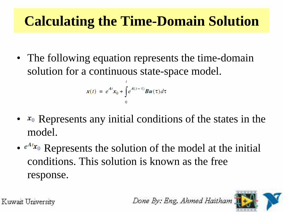
• The following equation represents the time-domain solution for a continuous state-space model.

• Represents any initial conditions of the states in the model.

• Represents the solution of the model at the initial conditions. This solution is known as the free response.

Calculating the Time-Domain Solution

• Represents the state response for stable systems over time as the inputs drive the dynamic system from time

• This solution is the forced response. • The following equation represents the time-

domain solution for a discrete state-space model.

Calculating the Time-Domain Solution

• In this equation, denotes the discrete free response.

• denotes the discrete forced response.

Analyzing a Step Response• The step response of a dynamic system measures how the

dynamic system responds to a step input signal. The following equations define a unit step input signal.

• The Control Design and Simulation Module contains two VIsto help you measure the step response of a system and then analyze that response. – The CD Step Response VI returns a graph of the step response. – The CD Parametric Time Response VI returns the following response

data that helps you analyze the step response.

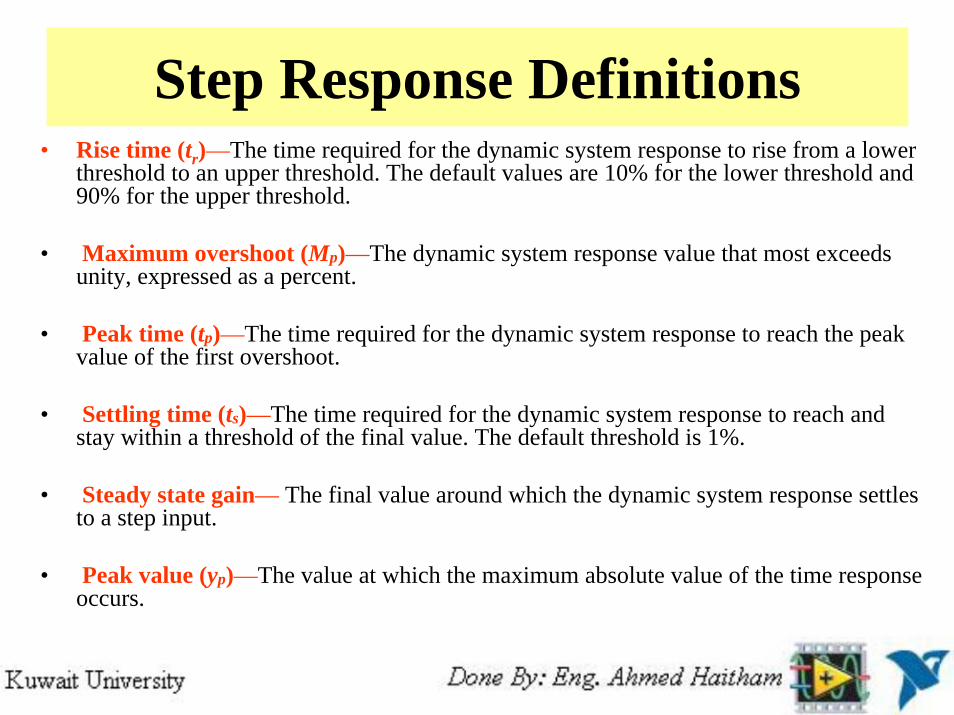
Step Response Definitions• Rise time (tr)—The time required for the dynamic system response to rise from a lower

threshold to an upper threshold. The default values are 10% for the lower threshold and 90% for the upper threshold.

• Maximum overshoot (Mp)—The dynamic system response value that most exceeds unity, expressed as a percent.

• Peak time (tp)—The time required for the dynamic system response to reach the peak value of the first overshoot.

• Settling time (ts)—The time required for the dynamic system response to reach and stay within a threshold of the final value. The default threshold is 1%.

• Steady state gain— The final value around which the dynamic system response settlesto a step input.

• Peak value (yp)—The value at which the maximum absolute value of the time response occurs.

Step Response Graph and Associated Parametric Response Data

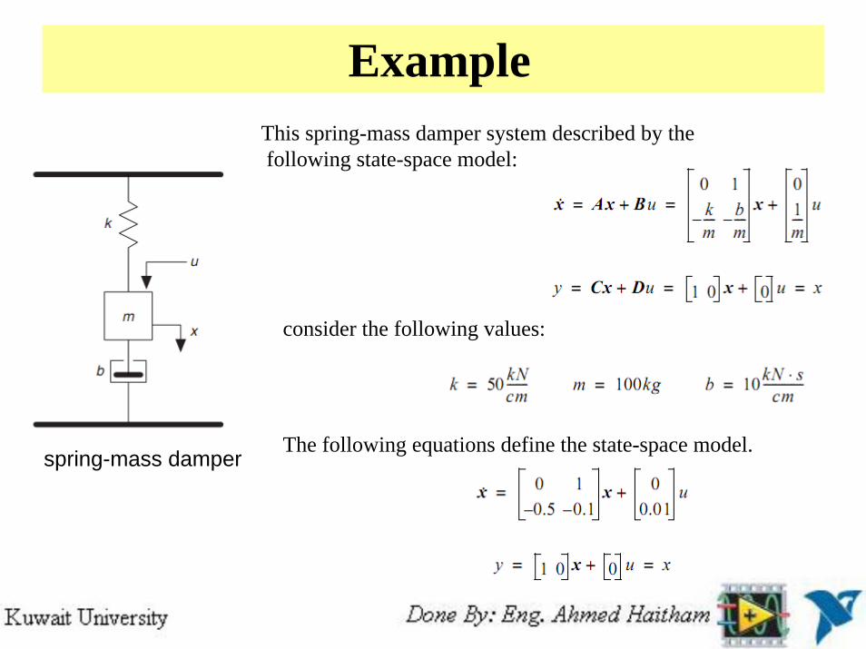
ExampleThis spring-mass damper system described by thefollowing state-space model:

consider the following values:

The following equations define the state-space model.spring-mass damper

Example

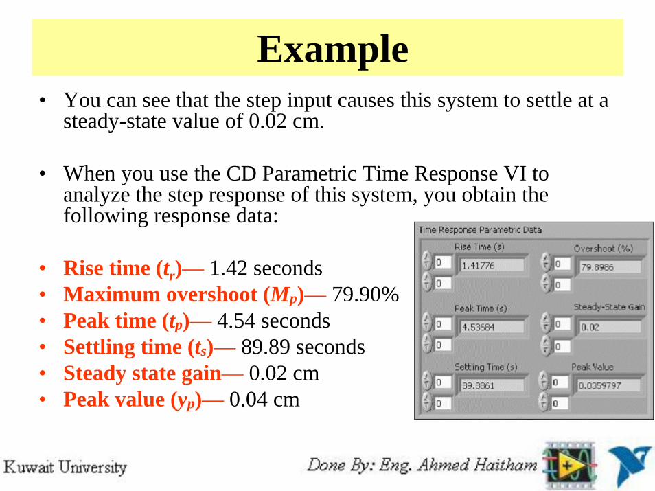
Example• You can see that the step input causes this system to settle at a

steady-state value of 0.02 cm.

• When you use the CD Parametric Time Response VI to analyze the step response of this system, you obtain the following response data:

• Rise time (tr)— 1.42 seconds • Maximum overshoot (Mp)— 79.90% • Peak time (tp)— 4.54 seconds • Settling time (ts)— 89.89 seconds • Steady state gain— 0.02 cm • Peak value (yp)— 0.04 cm

Analyzing an Impulse Response

• The impulse response of a dynamic system measures how the system responds to an impulse input signal. You define an impulse input signal in the following manner:

1. Continuous systems.Also known as the Dirac delta function

2. Discrete systems—Also known as the Kronecker delta function

• Use the CD Impulse Response VI to calculate the impulse response of a dynamic system to a standard impulse input.

Impulse Response Example

• Consider the system described in the Spring-Mass Damper Example

Analyzing an Initial Response

• The initial response of a dynamic system measures how the system responds to a set of non-zero initial conditions.

• Use the CD Initial Response VI to determine the initial response of a dynamic system.

Example• Consider the system described in the Spring-

Mass Damper Example

Analyzing a General Time-Domain Simulation• A general time-domain simulation of a system involves input signals that

are more general than step, impulse, or initial input signals.

• Use the CD Linear Simulation VI to solve these equations in response to an arbitrary input signal u into a system.

• This VI determines the response by numerically integrating these equations at the specified time steps. You can define the time steps with the Delta tinput

• The system model can be continuous or discrete, but the CD Linear Simulation VI converts continuous models to discrete models using either the exponential Zero-Order-Hold or the First-Order-Hold method.

• If this conversion is necessary, you must specify Delta t, which becomes the sampling time. If no conversion is necessary, Delta t must be equal to the sampling time of the output data u (t)

Example

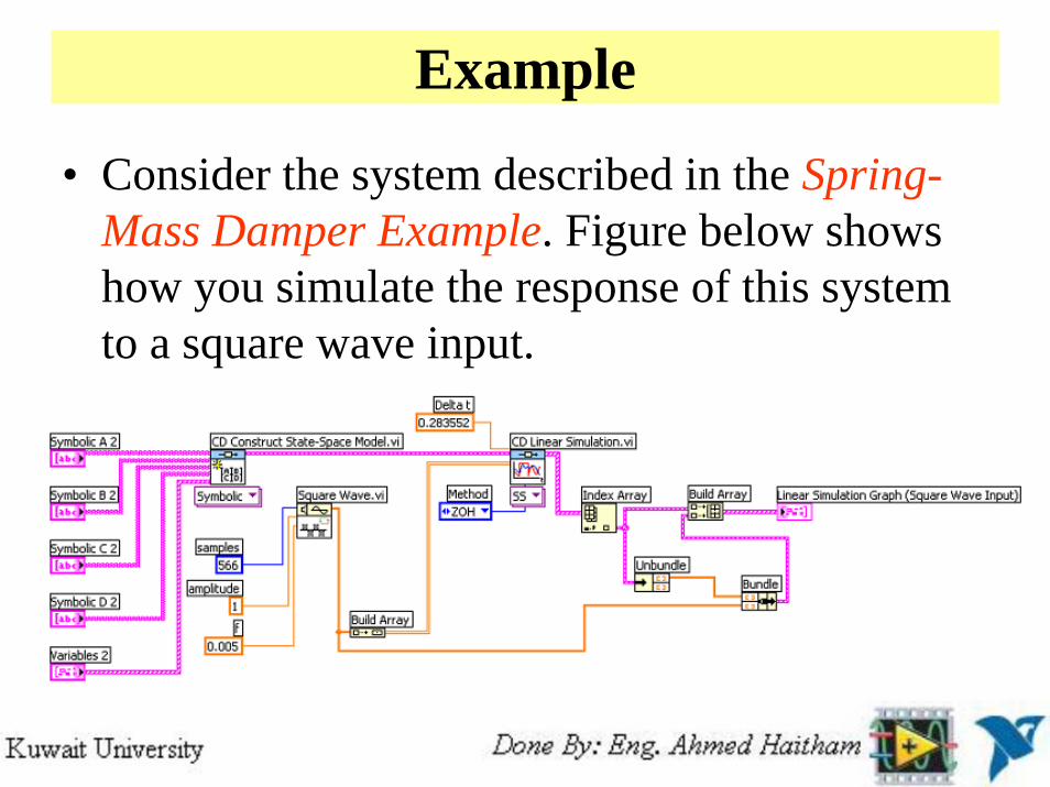
• Consider the system described in the Spring-Mass Damper Example. Figure below shows how you simulate the response of this system to a square wave input.

Example• Notice that the CD Linear Simulation VI converts the

continuous state-space model to a discrete model using the Zero-Order-Hold method. This conversion uses a Delta t input of approximately 0.3. This block diagram bundles the state-space model and the square wave as the input to the Linear Simulation Graph.

Obtaining Time Response Data

• The Time Response VIs return time response data that contains information about the time response of all input-output pairs in the model.

• Use the CD Get Time Response Data VI to access this information for a specified input-output pair, a list of input-output pairs, or all input-output pairs of the system.

2nd Order SystemExample Description:

This example demonstrates how to adjust the parameters and simulate the response of a continuous second order system. The adjustable parameters are the damping ratio, natural frequency (rad/s), gain, delay (s) and sampling time (s).