characteristics and mechanisms emissions

CHARACTERISTICS AND MECHANISMS OF

SPONTANEOUS OTOACOUSTIC EMISSIONS

STELLING EN

1. Volgens Furst {1989) geeft het passieve cochlea-model van

Furst en Lapid {1988) een adequate beschrijving van de statistische eigenschappen van spontane otoakoestische emissies. Deze conclusie is gebaseerd op onjuiste aannames.

Furst, M., and Lapid, M. (1988). A cochlear model for spontaneous otoacoustic emissions. J. Acoust. Soc. Am. 84, 222-229.

Furst, M. (1989). Reply to "Comment on 'A cochlear model for acoustic emissions'" [J. Acoust. Soc. Am. 85, 2217(1989)]. J.

Acoust. Soc. Am. 85, 2218-2220.

2. Ret opwekken van akoestische emissies met een door het binnenoor gestuurde wisselstroom is geen bewijs voor het

bestaan van een omgekeerd transduktieproces in het binnenoor.

Mountain, D.C., and Hubbard A.E. (1989). Rapid force production

in the cochlea. Hear. Res. 42, 195-202.

3. De weerstand van enkele gehoorsonderzoekers tegen de hypothese dat het oor gebruik maakt van actieve filters strookt

niet met de consensus over de hypothese dat door de Evolutie

biologische processen worden geoptimaliseerd.

4. De door lokale calorische stimulatie van een booggang

opgewekte responsie van het evenwichtsorgaan wordt niet uitsluitend veroorzaakt door vloeistofstroming in de booggang

onder invloed van de zwaartekracht.

von Baumgarten, R., et al. (1984). Effects of rectilinear acceleration and optokinetic and caloric stimulations in space. Science 225, 208-212.

Wit, H.P., Spoelstra, H.A.A. en Segenhout, J.M. (1989). Barany's

theory is right, but incomplete. An experimental study in pigeons.

Acta Otolaryngol. (Stockh.), aangeboden voor publikatie.

5. Recent morfologisch onderzoek van de maculae van de rat

suggereert dat reeds in deze zintuigepithelen van het

------------

evenwichtsorgaan gedistribueerde parallelle signaalverwerking plaats vindt. Dit betekent dat gangbare beschrijvingen van de

werking van het evenwichtsorgaan te eenvoudig zijn.

Ross, D.R. (1988). Morphological evidence for parallel processing of

information in the rat macula. Acta Otolaryngol. (Stockh.) 106, 213-218.

6. Volgens Volkov was Dmitri Sjostakowitsj op de hoogte van de publicatie van zijn eigen 'memoires'. De enige concrete

aanwijzing voor de juistheid van deze bewering is de verklaring van Volkov zelf.

Volkov, S. {1979). Testimony. The memoirs of Dmitri Shostakovitsj,

as related to and edited by Solomon Volkov (Faber and Faber, London).

7. In verband met de slechte akoestiek in cafetaria's, is de

slechthorende gebaat bij het gebruik in dergelijke

eetgelegenheden van plastic wegwerpbestek in plaats van metalen bestek.

8. Door het openbreken van het IJzeren Gordijn zal binnen

afzienbare tijd het bezit van een Lada automobiel zijn exclusiviteit verliezen.

9. De opvatting dat stellingen bij een proefschrift bedoeld zijn om frustraties te etaleren, is een wijdverbreid misverstand.

10. Een promovendus uit in zijn stellingen soms zijn frustraties.

Pim van Dijk

maart 1990

RIJKSUNIVERSITEIT GRONINGEN



Proefschrift

ter verkrijging van het doctoraat in de Wiskunde en Natuurwetenschappen aan de Rijksuniversiteit Groningen

op gezag van de Rector Magnificus Dr. L.J. Engels in het openbaar te verdedigen op

maandag 5 maart 1990 des namiddags te 4.00 uur

door

Pim van Dijk

geboren op 4 november 1960 te Delft

Eerste promotor: Prof. Dr. Ir. H.P. Wit Tweede promotor: Prof. Dr. Ir. H. Duifhuis

UNIVERSITY OF GRONINGEN The Nether lands



Thesis

submitted to fulfil the requirements of the Ph.D. degree in Mathematics and Nat ural Sciences

on the authority of the Rector Magnificus Dr. L.J. Engels

to be defended in public on Monday, March 5th, 1990

at 4.00 p.m.

by

Pim van Dijk

born on november 4, 1960 in Delft, The Netherlands

Aan mijn ouders

� krips repro meppel

The experiments described in this thesis were performed at the Institute of Audiology, University Hospital, P.O.Box 30.001, 9700 RB Groningen, The Netherlands (Chapter 1, 2, and 3), and the Electronics Research Laboratorium, University of California, Berkeley, CA 94720, USA (Chapter 4).

This work was supported by the Netherlands Organization for Scientific Research (NWO) through the Foundation for Biophysics.

Contents

INTRODUCTION 1

Chapter 1 7 SYNCHRONIZATION OF SPONTANEOUS OTOACOUSTIC EMISSIONS TO A 2jl - f2 DISTORTION PRODUCT.

P. van Dijk and H.P. Wit, submitted to J . Acoust . Soc. Am . .

Chapter 2 23 AMPLITUDE AND FREQUENCY FLUCTUATIONS OF

SPONTANEOUS OTOACOUSTIC EMISSIONS. P. van Dijk and H.P. Wit , submitted to J . Acoust . Soc. Am . .

Chapter 3 65 SPONTANEOUS OTOACOUSTIC EMISSIONS IN THE EUROPEAN

EDIBLE FROG ( R ANA ESCULENTA) ; SPECTRAL DETAILS AND TEMPERATURE DEPENDENCE.

P. van Dijk, H.P. Wit and J .M. Segenhout , Hear. Res. 42, 273-282.

Chapter 4 TEMPERATURE EFFECTS ON AUDITORY NERVE FIBER

RESPONSE IN THE AMERICAN BULLFROG.

P. van Dijk, E.R. Lewis and H.P. Wit, Hear. Res. , accepted.

SAMENVATTING

NAWOORD

87

107

113

INTRODUCTION

The discovery of otoacoustic emissions (Kemp, 1978) has fundamentally changed the view of hearing researchers on the function of the inner ear.

Before 1978, the ear was considered to be a oneway system: Sound from the surrounding world hits the tympanic membrane, located in the external ear canal. The middle ear bones transmit the vibration of the tympanic membrane to the fluids of the inner ear. Vibration of the inner ear fluids results in a traveling wave along the basilar membrane. Finally, the haircells, located on the basilar membrane transduce the mechanical vibration into electrical signals which exit the ear through the nerve fibers. Primary stimulus for the haircells is deflection of the hairs (stereocilia) on top of the cell (Hudspeth, 1989). In this detection scheme acoustical energy flows in one direction: from outer world to nerve fiber.

However, in 1978, Kemp reported that in response to a click presented to the ear, a weak acoustical signal could be detected in the ear canal. Thus, apparently the ear can also emit acoustical energy. i .e. energy can flow in the opposite direction. From this first publication on the topic it was clear that, what was later termed 'Kemp-echo', is not just an ordinary echo. For example, the time between the click stimulus and the 'echo' is too long to be a simple round-trip of the click. Also, the 'echo' intensity does not grow linearly with increasing click intensity, as would be expected for ordinary reflection of sound.

Initially, Kemp's results were taken with skepticism. For example, Wilson (1984), who later contributed substantially to the emission literature, writes that his 'interest in the phenomenon arose out of an attempt to discover the source of the "artefact" ' . The first confirmation of Kemp's results came from Groningen (Wit and Ritsma, 1979)

1

and was soon followed by many others. Shortly after the 'Kemp-echo' or click evoked otoacoustic emission,

the spontaneous otoacoustic emission was discovered (Kemp, 1979; Wilson, 1980; Zurek, 1981 ): with a sensitive microphone connected to a subjects ear canal, one or more stable tones with different frequencies may be recorded in absence of any acoustical stimulation. A recorded emission, played back on a tape deck, sounds like a continuous whistle with fixed frequency and loudness. Frequency and loudness of spontaneous otoacoustic emissions appear to be approximately constant over years. The spontaneous otoacoustic emission showed that the inner ear can generate acoustical energy, without any acoustical stimulation.

Following its discovery, hearing researchers wondered what would be the role of otoacoustic emissions in hearing mechanisms. There is a considerable amount of evidence that otoacoustic emissions indeed have something to do with these mechanisms. We will mention three pieces of evidence:

Firstly, otoacoustic emissions occur rarely in hearing impaired ears, while evoked and spontaneous emissions are measured with respectively 95 % (Bonfils et al., 1987) and 30 % (Dallmayr, 1985) incidence in normal hearing ears. Evidently, the emission phenomenon is related to normal hearing.

Secondly, emission frequencies appear to be related to local minima in the audiogram. The audiogram is a plot of frequency vs. pure tone threshold. For tones with various frequencies, the audiogram displays the intensity needed to let the tone be just audible for a subject . It was known for some time, that the audiogram exhibits very sharp local minima at certain frequencies. All spontaneous emission frequencies appeared to coincide with threshold minima (Wilson, 1980). So, the ear is most sensitive to tones with a frequency close to an emission frequency. On the other hand, not all threshold minima coincide with an emission frequency. So apparently, a threshold minimum is not caused by the presence of an emission. Rather, they seem to have a common source, which indicates that emission generation is indeed linked to hearing mechanisms.

Finally, we mention the relation between hearing threshold and emission intensity. After exposure for several minutes to loud sound,

2

the sensitivity of the ear is temporary reduced. This can be experienced by anyone who visits pop-concerts. Zwicker (1983) showed that parallel to this threshold elevation, the intensity of evoked emissions was temporary reduced. Again, this example indicates correlation between hearing mechanisms and emission generation. Moreover, it shows that the generation of emissions is related to optimal functioning of the ear.

The above examples illustrate the relation of otoacoustic emissions to signal detection in the ear. But, they give no clue as to the function of emissions in hearing. Up to the present day, the function of emissions have not been identified. However, most hearing researchers consider the existence of otoacoustic emissions as evidence for the use of active filtering by the ear. Why would the ear benefit from active filtering, and why would active filtering give rise to otoacoustic emissions?

Tracing back auditory literature reveals that the idea of active filtering has been brought up by Gold as long ago as 1948. Gold (1948) considered one of the most remarkable properties of the inner ear, its frequency selectivity. As Von Helmholtz (1862) postulated, the inner ear consists of an array of filters, tuned to successively increasing frequencies. Since two tones with different frequencies excite different filters, we are able to distinguish the frequency of both tones. A number of experiments have identified the coiled basilar membrane with the haircell rows located on it, as the frequency analyzing array.

Gold pointed out that the frequency selectivity of a filter is limited by damping, i.e. if damping increases, the frequency range to which the filter is sensitive also increases. From his own experiments, Gold estimated the width of the auditory filters to be about 20 Hz. As he pointed out , the viscosity of inner ear fluids would reduce the frequency selectivity of the filters to a much higher value than this 20 Hz. So he concluded that the narrow 20 Hz filters can not be accounted for by assuming the filters to be passive.

A standard scheme to increase the frequency selectivity of a filter, known from engineering, is the inclusion of a feedback loop in the system. The feedback loop connects the output of the filter back to its input . Using positive feedback, the effect of damping can be reduced. Damping extracts energy from the signal which is to be detected. So,

3

in order to compensate for the damping, energy must by supplied, i.e. the feedback loop must include an amplifier. Therefore, the resulting system is termed an active filter. Gold, proposed such an active filter for the auditory system. Also, Gold realized that a feedback system has an important drawback: if the energy supply in the feedback loop is too large, the system becomes unstable. This results in spontaneous oscillations: the filter will start to act as an oscillator. In his 1948 paper, Gold predicted the existence of otoacoustic emissions as a product of oscillating inner ear filters!

The discovery of otoacoustic emissions 30 years later (Kemp, 1978) has made active processes a key topic in auditory research. Experiments on emissions yield the possibility of investigating active processes in the inner ear, without changing the ears physiological condition.

A crucial experiment was performed by Bialek and Wit (1984) . They showed that the probability distribution of a spontaneous otoacoustic emission resembles that of a sinusoid. This result rejects the possibility that spontaneous otoacoustic emissions are generated by some noise source within the ear. It shows that otoacoustic emissions are generated by a selfsustaining oscillator in the ear, in agreement with the hypothesis that an emission is generated by an unstable active filter.

Chapter 1 and 2 of this thesis relate some properties of spontaneous otoacoustic emissions to existing theories on oscillators.

Chapter 1 describes synchronization of spontaneous otoacoustic emissions. Synchronization is a phenomenon typical of self-excited oscillators. If a periodic force is applied to an oscillator, the behaviour of the oscillator is conducted by a struggle between force (which tries to impose its frequency on the oscillator), and oscillator (which tries to maintain its own natural frequency) . A strong force will manage to synchronize the oscillator. If the oscillator is driven by a weak force, it will be able to maintain its own natural frequency. As has been described in Chapter 1, this behaviour is also observed for spontaneous otoacoustic emissions. However, at intermediate driving force levels, experiments show that an emission randomly jumps between its own natural frequency and the driving frequency. This indicates that apart from the driving force, the emission generator also interacts with some

4

noise source in the inner ear. A possible noise source is thermal noise in the inner ear. However, the experiments described in Chapter 1 do not yield information on the origin of the noise.

In Chapter 2 we describe the analysis of emission signals that were recorded without any acoustical stimulation. A spontaneous otoacoustic emission is a sinusoid with small fluctuations in amplitude and frequency. The observed fluctuations are interpreted in terms of a second order oscillator model. Fluctuations in the model are caused by a noise source that interacts with the oscillator. Comparison of experiment and theory yields information on oscillator and noise characteristics.

Otoacoustic emissions are also observed in various animals other than humans. In various other species, emissions occur at a small incidence rate. The only non-human animal which is known to have spontaneous emissions in number, is the frog. The occurrence of emissions in frogs is of special interest, since the structure of their inner ear is simple compared to that of humans. Still, the frog ear produces otoacoustic emissions. Apparently, the complexity found in the human ear is not necessary to explain emission generation.

Chapter 3 describes spontaneous emissions in the European edible frog. Since frogs are ectothermic animals, their body temperature follows environment temperature. Changing the frogs temperature offers a reversible method for investigating emissions. A major portion of Chapter 3 describes the temperature dependence of the level and the frequency of emissions.

Chapter 4 describes temperature effects on the response of auditory nerve fibers in the American bullfrog. Nerve fiber signals are the output of auditory filters in the ear. Since a nerve fiber contacts only a few haircells, it only responds to sound in a limited frequency range. The frequency to which a nerve fiber is most sensitive is called "best frequency" . Because we think that otoacoustic emissions and auditory filtering are related, we expected to see that emission frequency and best frequency change in a similar way as the temperature is changed. As is described in Chapter 4, this is not the case. So, the results in Chapter 4 do not provide extra evidence for the hypothesis that an emission is generated by an unstable auditory filter. On the other hand, the hypothesis is not contradicted. Auditory filters in the frog ear are known to be of high order, i.e. their frequency response is the

5

net result of the contribution of a large number (n rv 10) of components (Lewis, 1988). Possibly, an emission is generated by instability of a single component, while tuning is due to all components together. Then, emission frequency and best frequency do not necessarily have the same temperature dependence.

Bialek, W.S. , and Wit, H.P. (1984) Quantum limits to oscillator stability: theory and experiments on acoustic emissions from the human ear. Phys. Lett . 104A, 173-178.

Bonfils, P., Uziel, A. , and Pujol, R. (1987) Les oto-emissions acoustiques I. Les oto-emissions provoquees: une nouvelle technique d'exploration fonctionelle de la cochlee. Ann. Oto-Laryng. (Paris) 104, 353-360.

Dallmayr, C. (1985) Spontane otoakustische Emissionen, Statistik und Reaktion auf akustische Stortone. Acustica 59, 67-75.

Gold, T. (1948) Hearing II. The physical basis of the action of the cochlea. Proc. R. Soc. E. B135, 492-498.

Helmholtz, H. von (1862) Die Lehre von den Tonempfindung als Physiologische Grundlage ffu die Theorie der Musik. Vieweg und Sohn, Braunsweig.

Hudspeth, A.J. (1989) How the ear's works work. Nature 341, 397-404. Kemp, D.T. (1978) Stimulated acoustic emissions from within the human

auditory system. J . Acoust . Soc. Am. 64, 1386-1391. Kemp, D.T. (1979) Evidence of mechanical nonlinearity and frequency se

lective wave amplification in the cochlea. Arch. Otol. Rhinol. Laryngol. 224, 37-45.

Lewis, E.R. (1988) Tuning in the bullfrog ear. Biophys. J. 53, 441-447. Palmer, A.R., and Wilson, J .P. (1981 ) Spontaneous and evoked acoustic

emissions in the frog Rana esculenta. J. Physiol. (Lond.) 324, 64P. Wilson, J.P. (1980) Evidence for a cochlear origin for acoustic re-emissions,

threshold fine-structure and tonal tinnitus. Hear. Res. 2, 233-252. Wilson, J.P. (1984) Otoacoustic emissions and hearing mechanisms. Revue

Laryng. 105, Supplementum, 179-191 . Wit, H.P. , and Ritsma, R.J. (1979) Stimulated acoustic emissions from the

human ear. J. Acoust . Soc. Am. 66, 911-913. Zurek, P.M. (1981) Spontaneous narrowband acoustic signals emitted by

human ears . J. Acoust . Soc. Am. 69, 514-523. Zwicker, E. ( 1983) On peripheral processing in human hearing. In: R. Klinke

and R. Hartmann (Eds.) Hearing - Physiological Bases and Psychophysics, Springer, Berlin, pp. 104-110.

6

Chapter 1

SYNCHRONIZATION OF SPONTANEOUS OTOACOUSTIC EMISSIONS TO A 2/1 - /2 DISTORTION PRODUCT

Abstract

Synchronization of spontaneous otoacoustic emissions to a cubic distortion frequency is = 2i1 - i2 has been studied. The stimulus, consisting of two primary tones at frequency i1 and i2, could easily be filtered out of the microphone signal. This enabled us to monitor emission phase with respect to synchronization frequency is , by recording zerocrossing moments of the microphone signal. When primaries were sufficiently loud (typically 30 dB SPL) , phase fluctuated around a constant value: the emission was constantly synchronized to is · Lowering primary levels (to typically 20 dB SPL) , resulted in 211"phase jumps at random moments: the emission occasionally slipped out of synchronization, trying to maintain its own natural frequency io · This behaviour can be described as synchronization of an oscillator (frequency io) to a sinusoidal force (frequency is ) , in the presence of nmse.

Introduction

Two coupled oscillators with different frequency, tend to synchronize each other. This phenomenon has probably first been described by Christiaan Huygens (1893). In a letter to his father, he expressed astonishment about his observation, that the pendulums of two clocks, attached next to each other on the same wall, exhibited a synchronous motion. Even when de-synchronizing the pendulums by a slight hand

7

push, the synchronized regime re-occurred after a small amount of time. Apparently, the slight click, produced by each clock was transmitted through the wall, and was sufficient to synchronize the clocks.

Synchronization is a phenomenon typical for the interaction of an oscillator with a periodic force. The external force tries to impose its frequency on the oscillator, while the oscillator will try to maintain its own natural frequency.

In this work, we report on synchronization of spontaneous otoacoustic emissions (SOAE) . An SOAE can be synchronized to a single tone presented to the ear, with frequency close to the emission frequency (Wilson and Sutton, 1981; Zwicker and Schloth, 1984; Bialek and Wit , 1984; Long, 1986; Long et al. , 1988; Tubis et al. , 1988). Similar to the example described above, synchronization may be caused by a very weak driving force. Wit and Ritsma (1983) showed that synchronization of an emission can be induced by a tonal pulse carrying approximately 0.5 e V of energy.

In synchronization experiments, typically, a subjects ear canal is sealed off by an acoustic probe containing (1) a small earphone to present the stimulus, and (2) a sensitive microphone to record ear canal sound pressure. Consequently, stimulus and emission are both picked up by the microphone. A disadvantage of studying synchronization of SOAE's with a single sinusoidal tone is, that stimulus and emission in the recorded microphone signal cannot be separated. Therefore, we studied synchronization of SOAE's to a 2/1 - /2 distortion product , generated in the ear by two sinusoidal stimuli with frequency ft and /2• Then, the stimulus (i.e. the sinusoidal tones) can easily be separated from the emission signal by filtering. Using zerocrossings of the filtered microphone signal, we were able to study phase behaviour of the emission in detail.

Before describing the results, we will first review synchronization of a theoretical oscillator, and will pay special attention to its phase behaviour.

Theory

From a mathematical point of view, the simplest self-exciting oscillator is the Van der Pol oscillator (van der Pol, 1927; Guckenheimer

8

and Holmes, 1986) . We will consider the interaction of a Van der Pol oscillator with a sinusoidal external force, in the presence of noise. This problem has been extensively treated by Stratonovich ( 1963). We will briefly review his results. (See, for a tutorial paper on selfexciting oscillators, Hanggi and Riseborough (1982)).

The equation of motion of the Van der Pol oscillator, interacting with external force E sin 2nJ.t and noise force hF(t) is:

mx + ( -R1 + R2x2)i: + K-x = E sin2nJ,t + hF(t) (1.1)

with R1 > 0 and R2 > 0. We will assume that R1 � ( K-m )112 • Then, in absence of noise ( h F( t) = 0) and external force ( E = 0), the oscillator will approximately exhibit a sinusoidal motion:

x(t) = A0 cos(2n'f0t + </>0) (1.2)

with: A0 = 2 {R;R1

and fo = _!_ {K v R; 27r v -:;;;

The external force, tries to impose its frequency f, on the oscillator, i.e. tries to synchronize the oscillator. This force also affects the amplitude of x(t) . The random force causes random amplitude and frequency fluctuations of oscillation x(t). If both the external force is weak (E � 27r J.R1A0), and the noise force is weak (i.e.noise power spectral density S6F(f,) � 167r2mJ; A�Rt), amplitude of x(t) is not effected very much. Then, the solution of eq. (1.1) can approximately be written as:

x(t) = A0 cos [27rj11t + </>(t) ] (1.3) Phase </>(t) with respect to driving frequency f. is the solution of:

if>= D -D. sin </> + e(t) (1.4)

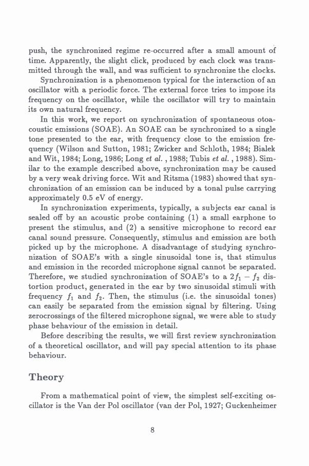
where, D = 21r(f0 - f. ), D. = -E/(47rf.mA0), and e(t) = -(27rf.A0t1 x hF(t) cos(21rj,t + </>). Equation (1.4) resembles the equation of motion of a massless particle, in a corrugated inclining potential V(</>) = -D</> -D. cos </>. Fig.1 shows V(</>) forD < O, i.e. fo < f • . The potential tries to stabilize the particle at one of its minima Pi . The noise "force" e(t) however, pushes the particle out the stable point . Occasionally, the noise force will manage to kick the particle into an adjacent potential valley. Such an event corresponds to a

9

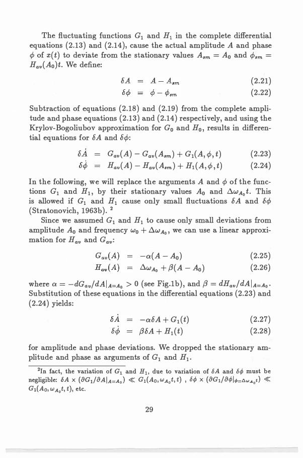
...... e > • iii ; c:: Q) -0 a. •

-2n 0 2n phase CD (rad)

Figure 1 : "Potential function" corresponding to phase equation (1 .4), for D < 0, i.e. fo < fa· The potential tries to stable the phase in one of its stable points Pt, P2, etc . .

temporal slip from synchronization of the oscillator. These 21r-jumps will be very rare, if Da/ D is large. Then, the potential valleys are deep, and the particle will reside almost continually in the same valley. This situation corresponds to a strong external force, which is able to almost constantly synchronize the oscillator to the driving frequency fa· On the other hand, for small Da/ D, the valleys in the potential are shallow, and 21r-jumps occur more often. Then, the external force is not able to continuously synchronize the oscillator. Moreover, for

D � D 5, the valleys in V ( ¢) have disappeared completely, and the "particle" will continuously slide along the inclining potential. Then, the driving force is too weak, and synchronization of the oscillator is not possible.

If the correlation time 'Tcor of the noise source is short ( 'Tcor � m/ R1), solving the Fokker-Planck equation corresponding to eq. (1.4) yields a stationary phase probability distribution w( ¢ ) :

1 r<�>+21r 1

w (¢) = Ce(D<f>+D,cos<f>)/,;do }</> e-(D.P+D,cos,P)/,;dod'l/J (1 .5)

where do = s6F(/s)/(167r2m2 r; A�), and cis determined by the nor-

10

malization condition J:'lr w( </> )d¢ = 1. In absence of the driving force, phase is uniformly distributed: w(D3 = OJ¢) = (27r)-1. Due to the driving force, phase is more likely to be in the valleys, than on the hills of the corrugated potential V(¢) (see Fig.1). We define width fl.¢ of the phase distribution as !::!..¢ = </>2- ¢11 where w( </>1,2) = (27r)-1• Using eq. (1.5), width fl.¢ can be calculated. For fixed D, fl.¢ is a monotonously decreasing function of D 11•

The 27r-phase jumps result in an average frequency (f) different from j11:

1 . 1 1 (f) = J. + -(¢) = J. + -D- -D.(sin ¢) (1.6) 211" 211" 211"

where (sin ¢) = Jg1r sin</> w( </> )d¢. As an example, we consider fo < J�� (i.e. D < O, see Fig.1). Due to the inclination of V(¢), a phase jump in negative ¢-direction is more likely to occur than a positive-going jump. Therefore, (¢) < 0, and (f) < j,.. In absence of a driving force, (sin ¢) = O, and average frequency is maximally shifted away from j11: (f) = f�� + (27r)-1 D = fo ·

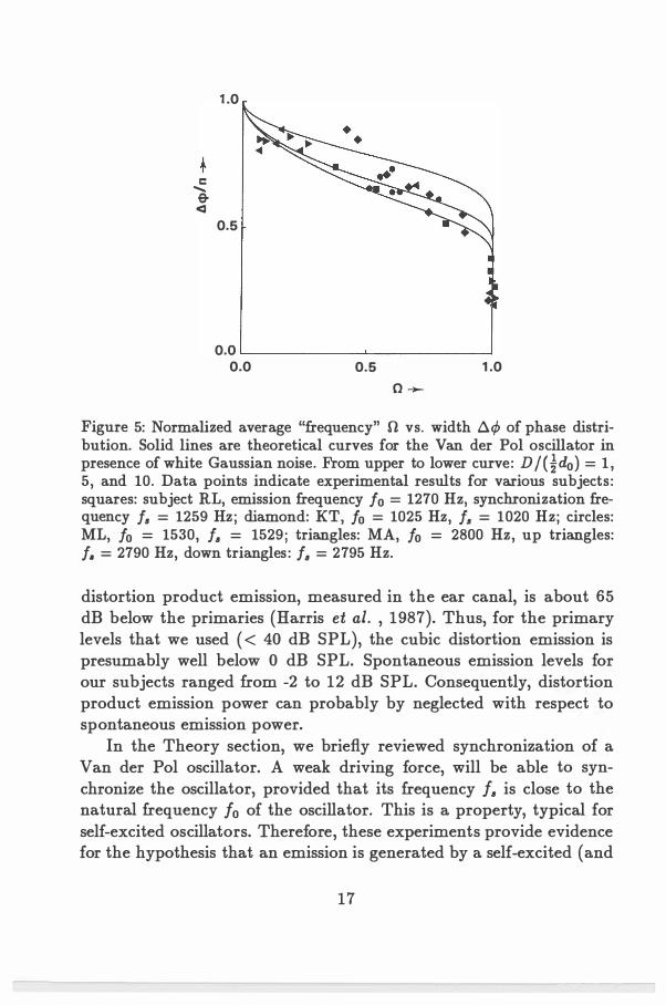
Using equations (1.5) and (1.6), we computed width !::!..¢ and frequency (f) for various D/ldo, and D��/ld0• Solid lines in Fig. 4 display normalized average "frequency" n = ( (f) - fo)/(J/J - fo) vs. 6.¢ for Dj�d0 = 1, 5 and 10. For strong driving force, n approaches 1, and 6.¢ approaches 0. For weak driving force, n approaches o, and 6.¢ approaches 1r.

Since phase will gradually slide down the potential V( </>),the power spectrum S:�:(f) of x(t) will be asymmetric. Sz(J) consists of a 6-function peak at f = j3 and a broad continuous peak with center frequency fc and width b..fc· Consider for example fo < j6• Then, with increasing D11, (1) frequency fc monotonically increases from fo (for D11 = 0) to j11, and (2) 6.fc monotonically increases from minimum 27rdo (for D. = 0).

Material and Methods

Experiments were performed in 4 ears of 4 human subjects, with at least 1 spontaneous otoacoustic emission (frequency f0). Sound pressure level of this emission was -2, 3, 11 and 12 dB SPL, for subject RL, MA, ML and KT respectively.

11

An acoustic probe was connected to the subject's ear canal. The probe contained a sensitive condenser microphone (Wit et al., 1981) and two earphones.

The earphones were used to generate simultaneously two pure tone stimuli. For various frequencies /1 and /2 and levels L1 and L2 of the primaries, the microphone signal was recorded on channel 1 of a Sony SL-C30E video recorder, after pulse code modulation (Sony PCM-F1). For each stimulus condition record length was 80 s.

Frequency difference /2 -/1 was fixed for each individual subject, and ranged from 150 to 300 Hz across subjects. Frequencies /1 and /2 were chosen to yield a the cubic distortion frequency/. =2ft-/2 less than 25 Hz from emission frequency /0• For each subject 2 or 3 frequencies Is were used.

Primary levels L1 and L2 used ranged from 17 to 39 dB SPL. For subjects MA, RL and KT, the difference L2 - L1 was fixed at respectively +1, +4 and -3 dB. For subject ML, L1 = 29 dB SPL was fixed, and only L2 was varied. Suppression of the emission by the primaries was always less than 3 dB.

During a recording session, consecutive stimulus levels were chosen quasi random, i.e. not either systematically increasing or decreasing. Typically, after having recorded for three different stimulus conditions, a record was taken of the microphone signal in absence of primaries. This enabled us to monitor slight shifts of emission frequency and level, which usually occurred during recording sessions.

Simultaneously with the microphone signal, a reference tone with frequency /. was recorded on the second channel of the tape recorder. This reference was generated externally, using the outputs of the sinewave synthesizers that generated the primary frequencies /1 and 12·

To each 80 s record, the following analysis procedures were applied: The phase behaviour of a spontaneous otoacoustic emission could

be monitored after bandpass filtering the recorded microphone signal, using a Briiel & Kj�r 2020 heterodyne filter with 31.6 Hz bandwidth. This reduced the influence of microphone noise. Center frequency of the filter was set in such a way that both f. and /0 fell within the passband.

We used a HP 5326A timer to measure time intervals llti between

12

the i-th zero-crossing of the reference signal (channel 2) and the consecutive zero crossing of the filtered microphone signal (channel 1 ) . Successive !:iti were stored on computer disk. Phase of the emission with respect to the reference signal was calculated with </>i = 27r /6/:iti. Recorded phase traces were used to compute a phase probability distribution w(¢), with J�71' w(¢)d¢ = 1 . For each distribution, width 1:1¢ at w ( ¢) = 1/ ( 27r) was determined. Also, average emission frequency (f) was determined from the average frequency Jij- of positive- and negative-going 21r-jumps visible in the phase trace: (f) = /6+ f:frr-/2�. From average frequency, we determined normalized average frequency n = ( (f) - !o)!Ua - !o) ·

Averaged power spectra (n = 8) of recorded microphone signals were determined, using a Unigon 4512 FFT analyzer. In order to get a 0.2 Hz frequency resolution, spectra were zoomed in on a 100 Hz frequency region around the emission frequency. Zoomed spectra contained a narrow peak at fa and/or a broader peak near frequency fo of the unstimulated emission. From the area covered by a peak, its sound pressure level was determined. The broader peak was fitted to a Lorenzian curve S(f) = A/(!; + �!:if;) , which yields frequency fc , full width at half maximum (FWHM) l:ifc, and area 27r A/ l:ifc ·

Results

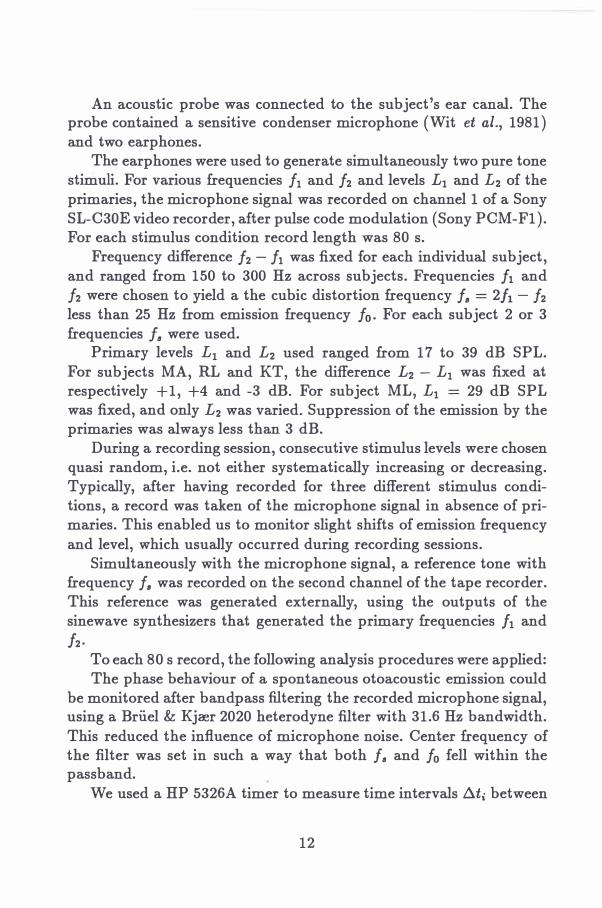
Fig. 2 displays three phase traces as recorded for subject RL. If the primary tones were strong enough, the emission phase fluctuated around a constant value (upper panel) . I.e., the emission was synchronized to cubic distortion frequency /6 = 2/1 - /2• Lowering primary levels causes the phase occasionally to make a 27r phase jump, i.e. to slide out of synchronization (middle panel). Decreasing the primary levels still further resulted in increase of number of 27r phase jumps. At low stimulus levels, emission phase slides off most of the time (lower panel).

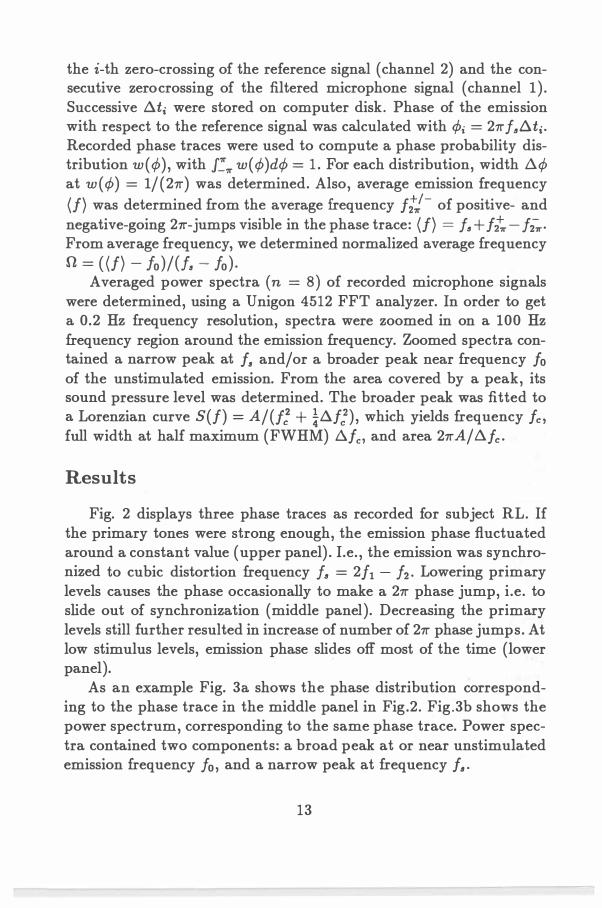
As an example Fig. 3a shows the phase distribution corresponding to the phase trace in the middle panel in Fig.2. Fig.3b shows the power spectrum, corresponding to the same phase trace. Power spectra contained two components: a broad peak at or near unstimulated emission frequency /0 , and a narrow peak at frequency f •.

13

2n

L1 = 27dB SPL

OL-------------�------------��------------�

_ 2n "'C as ... -Q) rn as

.c � OL-�--------��--�--------�----------�--�

2n

o�------�--��----��--��----------�� 0.0 0.5 1.0 1.5 time (s)

Figure 2: Phase traces, as recorded for subject RL. Emission frequency: /o = 1270 Hz, Synchronizing frequency: /. = 2/t - h = 1279 Hz. Primary frequencies were It = 1429 Hz, and fa = 1579 Hz. Primary level L1 is indicated in the Figure. Primary level L2 was 4 dB above L1 . Lowering primary levels resulted in an increasing number of 21r-jumps of emission phase.

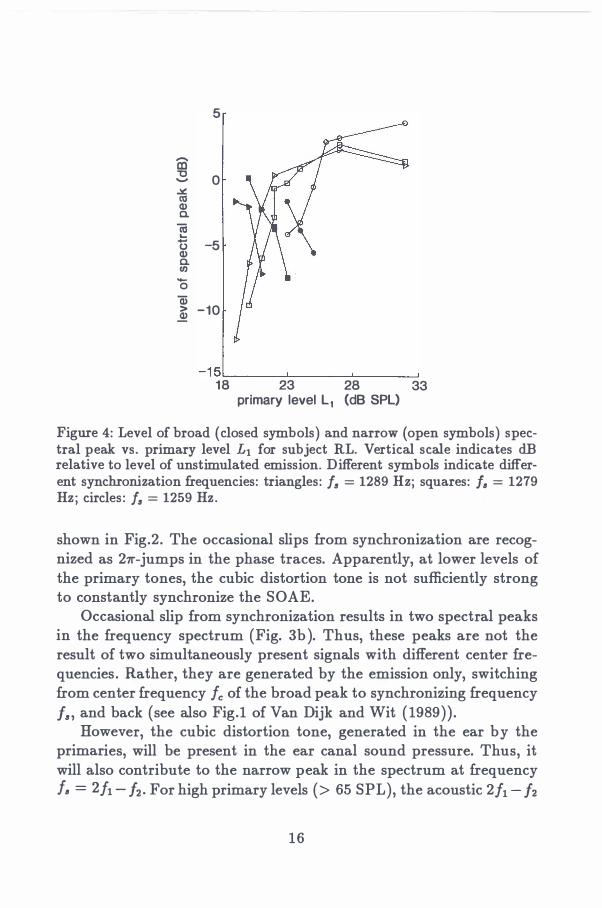
Increase of stimulus level resulted in: (1) decrease of the width 1::1¢ of the phase distribution, (2) increase of level of the narrow peak, (3) a decrease of level of the broad peak, and ( 4) an increase of the width !:if of the broad peak. Level of both spectral peaks as function of primary levels is shown in Fig.4 for subject RL. In all experiments, the sum of both levels, changed less then 5 dB. Width of the broad peak ranged from 0.15 to 1.5 Hz in absence of stimuli, to about 10 Hz when the peak was just separable from the microphone noise floor.

Fig.5 shows normalized average emission frequency n vs. width 1::1¢ of the emission phase distribution. Decrease of !:1.¢ (due to increase of primary levels), coincides with increase of normalized frequency. This

14

(a) 0.8

� "" 1 0.6 � "' c: Cll 0.4 ..., � :s ., 0.2 1

n phase (rad)

30

2n

(b)

e.,� 0 1270 1290

frequency (Hz)

Figure 3: (a) Phase probability density, corresponding to the middle panel in Fig.2. Width of this distribution is t:t..¢1 = 0.511". (b) Power spectrum of emission recording, corresponding to middle panel in Fig.2. Spectrum consists of a broad peak (open symbols) and a narrow peak at f = f. (closed symbols, connected by straight lines) . Smooth solid line is a Lorenz fit to the open symbols: center frequency fc = 1267 Hz, full width at half maximum (FWHM): tl.fc = 9 Hz. Levels relative to level of unstimulated emission were -3.6 dB and -2.9 dB for broad and narrow peak respectively.

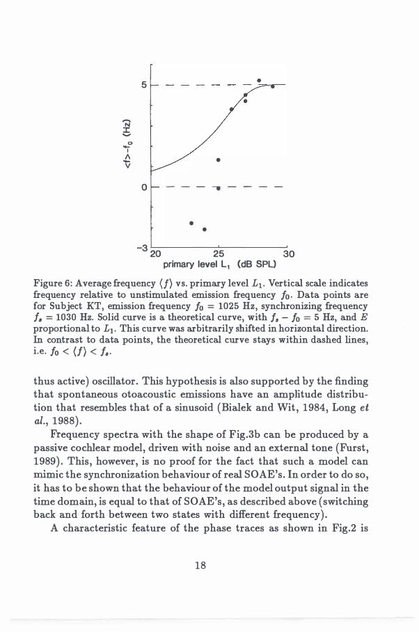
plot only shows results for f. < f0 • As an example of stimulus condition f. > f0, Fig.6 shows stimulus

level vs. average frequency for subject KT. For low stimulus levels, average frequency was smaller than /0 , corresponding to !l < 0 . Upon increase of stimulus, average frequency increased up to (f) = J. , i.e. !l = l .

Discussion

Two simultaneously presented sinusoidal stimuli, with frequency /1 and /2 respectively, are known to generate audible distortion products in the inner ear (von Helmholtz, 1862; Zwicker, 1955; Goldstein, 1966; Hall, 1972; Smoorenburg, 1972). We showed, that a spontaneous otoacoustic emission can be synchronized to frequency f. = 2/1 -/2, when the primary tones are sufficiently loud.

Lowering primary tone levels resulted in occasional slip from synchronization of the emission. This is illustrated by the phase traces

15

-Ill "'0 -� tU Q) a. (ij .... -() Q) a. en -0 Q) > �

5

0

-5

-10

-15L------L------�----� 18 23 28 33 primary level L1 (dB SPL)

Figure 4: Level of broad (closed symbols) and narrow (open symbols) spectral peak vs. primary level Lt for subject RL. Vertical scale indicates dB relative to level of unstimulated emission. Different symbols indicate different synchronization frequencies: triangles: /3 = 1289 Hz; squares: fll = 1279 Hz; circles: /3 = 1259 Hz.

shown in Fig.2. The occasional slips from synchronization are recognized as 27r-jumps in the phase traces. Apparently, at lower levels of the primary tones, the cubic distortion tone is not sufficiently strong to constantly synchronize the SOAE.

Occasional slip from synchronization results in two spectral peaks in the frequency spectrum (Fig. 3b ). Thus, these peaks are not the result of two simultaneously present signals with different center frequencies . Rather, they are generated by the emission only, switching from center frequency fc of the broad peak to synchronizing frequency /3 , and back (see also Fig.1 of Van Dijk and Wit (1989)) .

However, the cubic distortion tone, generated in the ear by the primaries, will be present in the ear canal sound pressure. Thus, it will also contribute to the narrow peak in the spectrum at frequency fll = 2ft- /2. For high primary levels (> 65 SPL), the acoustic 2ft - /2

16

c ....... & <I

1.0

0.5

0.0 '-----------'---------' 0.0 0.5 1.0

o--

Figure 5: Normalized average "frequency" n vs. width !J.¢> of phase distribution. Solid lines are theoretical curves for the Van der Pol oscillator in presence of white Gaussian noise. From upper to lower curve: D Jado) = 1, 5, and 10. Data points indicate experimental results for various subjects: squares: subject RL, emission frequency lo = 1270 Hz, synchronization frequency Is = 1259 Hz; diamond: KT, lo = 1025 Hz, Is = 1020 Hz; circles: ML, lo = 1530, 16 = 1529; triangles: MA, lo = 2800 Hz, up triangles: 1. = 2790 Hz, down triangles: 16 = 2795 Hz.

distortion product emission, measured in the ear canal, is about 65 dB below the primaries (Harris et al. , 1987). Thus, for the primary levels that we used ( < 40 dB SPL), the cubic distortion emission is presumably well below 0 dB SPL. Spontaneous emission levels for our subjects ranged from -2 to 12 dB SPL. Consequently, distortion product emission power can probably by neglected with respect to spontaneous emission power.

In the Theory section, we briefly reviewed synchronization of a Van der Pol oscillator. A weak driving force, will be able to synchronize the oscillator, provided that its frequency f6 is close to the natural frequency fo of the oscillator. This is a property, typical for self-excited oscillators. Therefore, these experiments provide evidence for the hypothesis that an emission is generated by a self-excited (and

17

'N ::c -

0 '"r " v

5

•

0 -----.----

• •

-3 20 25 30 primary level L1 (dB SPL)

Figure 6: Average frequency(!) vs. primary level Lt. Vertical scale indicates frequency relative to unstimulated emission frequency f0• Data points are for Subject KT, emission frequency fo = 1025 Hz, synchronizing frequency f. = 1030 Hz. Solid curve is a theoretical curve, with /11 - fo = 5 Hz, and E proportional to Lt. This curve was arbitrarily shifted in horizontal direction. In contrast to data points, the theoretical curve stays within dashed lines, i.e. fo < (f) < f.·

thus active) oscillator. This hypothesis is also supported by the finding that spontaneous otoacoustic emissions have an amplitude distribution that resembles that of a sinusoid (Bialek and Wit, 1984, Long et al., 1988) .

Frequency spectra with the shape of F ig.3b can be produced by a passive cochlear model, driven with noise and an external tone (Furst, 1989) . This, however, is no proof for the fact that such a model can mimic the synchronization behaviour of real SOAE's. In order to do so, it has to be shown that the behaviour of the model output signal in the time domain, is equal to that of SOAE's, as described above (switching back and forth between two states with different frequency).

A characteristic feature of the phase traces as shown in Fig.2 is

18

the randomness of 271"-jumps. Random slip from synchronization is also visible in data of Long et al. (1988) . They studied phase-lock of spontaneous otoacoustic emissions, using weak sinusoidal stimuli {down to -2 dB SPL ), and swept stimulus frequency across frequency of an emission. They recorded RMS sound pressure in the ear canal as function of stimulus frequency. If stimulus frequency is close the emission frequency, the emission is synchronized to the external tone. This is observed as an almost constant RMS sound pressure. If stimulus frequency is far away from emission frequency, the stimulus does not manage to synchronize the emission. Then emission frequency and stimulus frequency are simultaneously present in the ear canal sound pressure. This is observed as beating in the recorded RMS sound pressure. In the transition frequency region between constant synchronization and constant beating, some beats occur at random moments. Such a random beat can be interpreted as a random slip from synchronization of the emission, similar to the random 21r-phase jumps we observed in emission phase traces.

As has been shown in the Theory section, random phase jumps of an oscillator, can be modeled by introduction of a noise force in the equation of motion of the oscillator. Then, the phase behaviour of the oscillator is analogous to the motion of particle in an inclining corrugated potential (Fig.1 ) . The noise causes the particle to jump from one valley of the potential into an adjacent valley, at 271" distance. The dynamics of this particle, and thus the dynamics of emission phase ¢(t) , is determined by the shallowness of the potential. The shallowness of the potential is determined by the driving force amplitude (among other quantities) .

If we want to compare experiment and theory, it would be logical to compare quantities, related to phase behaviour, as function of driving force amplitude. A drawback of the present experimental technique is, that we do not have direct control on this amplitude, i.e. on amplitude of the cubic distortion tone. Therefore, we plotted n versus A¢ (Fig.5), rather than plotting each as function of stimulus (i.e. primary) levels.

Fig.5 shows experimental results and theoretical curves, calculated for a white Gaussian noise force. Agreement between theory and experiment is good. Van Dijk and Wit (1989) studied amplitude and

19

frequency fluctuations of SOAE's. They concluded that a Van der Pol oscillator driven by noise might be a good model for SOAE's. However, their data show that if the emission generator is assumed to be a Van der Pol oscillator, the noise cannot be white Gaussian noise. Therefore, the comparison made in Fig.5 between theory and experiment should be regarded as qualitative.

Fig.5 displays only results for is < io, i.e. synchronization frequency below emission frequency. Then, average frequency was always between emission frequency io and synchronization frequency is, and thus 0 < n < 1 . For i, > io average frequency could be below io (Fig.6), i.e. n < 0. This evidently can not be described by the Van der Pol oscillator, treated in the theory section. Negative n could be interpreted as a slight decrease of emission frequency io, due to the presence of the primary tones. This hypothesis is supported by experimental results of Rabinovich and Widin (1984) . They report frequency shift of an SOAE, caused by a single tone more then 200 Hz above the emission. At low stimulus level, which suppresses the emission less the 2 dB, they observed frequency shifts of about-2 Hz.

Acknowledgements

This work was supported by the Netherlands Organization for Scientific Research (NWO) and the Heinsius Houbolt Fund.

References

Bialek, W.S ., and Wit, H.P. (1984) . "Quantum limits to oscillator stability: theory and experiments on acoustic emissions from the human ear," Phys. Lett. 104A, 173-178.

Furst, M. (1989). "Reply to "Comment on 'A cochlear model for acoustic emission"' [J. Acoust . Soc. Am. 85, 2217 (1989)]," J. Acoust. Soc. Am.

85, 2218-2220. Goldstein, J .L. (1966). "Auditory nonlinearity," J. Acoust . Soc. Am. 41,

676-689. Guckenheimer, J., and Holmes, P. (1986) . Nonlinear Oscillators, Dynami

cal Systems, and Bifurcations of Vector Fields (Springer, New York), pp. 67-82.

Hall, J.L. (1972). "Auditory distortion products h- h and 2fi - /2," J . Acoust. Soc. Am . 51, 1863-171.

20

Hanggi, P., and Riseborough, P. (1982) . "Dynamics of nonlinear dissipative oscillators," Am. J. Phys. 51 , 347-352.

Harris , F .P. , Stagner, B.B. , Martin, G.K., and Lonsbury-Martin, B .L . (1987) . "Effect of frequency separation of primary tones on the amplitude of acoustic distortion products," J. Acoust . Soc. Am. 82, Suppl. 1, 5117.

Huygens, C . (1893). Letter to his father, Februari 26, 1665. In CEuvres completes de Christiaan Huygens, edited by the Societe Hollandaise des Sciences (Martinus Nijhoff, The Hague), Volume 5 , pp. 243.

Long, G.R. (1986) . "Synchronization of spontaneous otoacoustic emissions and driven limit-cycle oscillators," J. Acoust. Soc. Am. 79, Suppl. 1 , 55.

Long, G.R., Tubis, A. , Jones, K.L., and Sivaramakrishnan, S. (1988). "Modification of the external-tone synchronization and statistical properties of spontaneous otoacoustic emissions by aspirin consumption," in Basic Issues in Hearing, edited by H. Duifhuis, J.W. Horst and H.P. Wit (Academic Press, London) , pp. 93-100.

Rabinovich, W.M., and Widin, G.P. (1984) . "Interaction of spontaneous oto-acoustic emissions and external sounds," J. Acoust. Soc. Am. (76) , 1713-1720.

Schloth, E. and Zwicker, E. (1983) . "Mechanical and acoustical influences of spontaneous oto-acoustic emissions," Hear. Res. 11 , 285-293.

Smoorenburg, G.F. (1972). "Combination tones and their origin," J . Acoust . Soc. Am. 52, 615-632.

Stratonovich, R.L. (1963) . Topics in the Theory of Random Noise, Volume II, (Gordon and Breach, New York) , Chap . 9, pp. 222-276.

Tubis, A., Long, G.R., Sivaramakrishan, S . , and Jones, J.L. (1988) . "Tracking and interpretive models of the active-nonlinear cochlear response during reversible changes induces by aspirin consumption," in Cochlear Mechanisms: Structure, Function and Models, edited by D.T. Kemp and J .P. Wilson, (Plenum Press, New York) , in press.

van der Pol, B . (1927) . "Forced oscillation in a circuit with nonlinear resistance (receptance with reactive triode) ," London, Edinburg and Dublin Phil. Mag. 3, 65-80.

van Dijk, P., and Wit, H.P. (1987) . "Phase-lock of spontaneous otoacoustic emissions to a cubic difference tone," J. Acoust . Soc. Am. 82, Suppl. 1, 5117.

van Dijk, P., and Wit , H.P. (1988) . "Phase-lock of spontaneous otoacoustic emissions to a cubic difference tone," in Basic Issues in Hearing, edited by H. Duifhuis, J.W. Horst and H.P. Wit (Academic Press, London) , pp. 101-105.

van Dijk, P. , and Wit, H.P. (1989). "Amplitude and frequency fluctuation of spontaneous otoacoustic emissions," manuscript in preparation.

21

von Hehnholtz, H . (1862) . Die Lehre von den Tonempfindung als Physiologische Grundlage fiir die Theorie der Musik, (Vieweg und Sohn, Braunsweig) , Chap. 7 and Appendix 12 .

Wilson, J.P. , and Sutton, G.J. (1981) . "Acoustic correlates of tonal tinnitus," in Tinnitus, edited by D. Evered and G. Lawrenson (Pitman Books, London) , pp. 82-107.

Wit , H.P. (1986) . "Statistical properties of a strong otoacoustic emission," in Peripheral Auditory Mechanisms, edited by J.B. Allen, J.L. Hall, A. Hubbart , S .T. Neely and A. Tubis, (Springer Press, Berlin) , pp. 137-146.

Wit, H.P., Langevoort, J .C . and Ritsma, R.J . (1981) . "Frequency spectra of cochlear acoustic emissions ( 'Kemp-echoes') ," J. Acoust . Soc. Am. 70, 437-445.

Wit, H.P., and Ritsma, R.J. (1983) . "Sound emission from the ear triggered by single molecules? ," Neurosci. Lett . 40, 275-280.

Zwicker, E. (1955) . "Der ungewohnliche Amplitudengang der Nichtlinearen Verzerrungen des Ohres," Acustica 20, 206-209.

Zwicker, E., and, Schloth, E. (1984) . "Interrelation of different otoacoustic emissions," J . Acoust. Soc. Am. 75 , 1148-1154.

22

Chapter 2

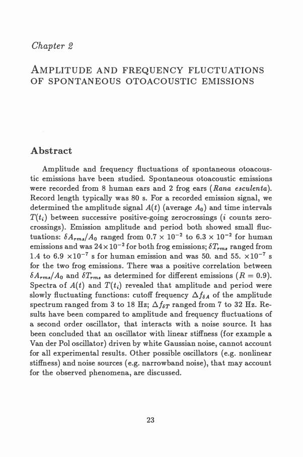
AMPLITUDE A ND FREQUENCY FLUCTUATIONS OF SPONTANEOUS OTOACOUSTIC EMISSIONS

Abstract

Amplitude and frequency fluctuations of spontaneous otoacoustic emissions have been studied. Spontaneous otoacoustic emissions were recorded from 8 human ears and 2 frog ears (Rana esculenta). Record length typically was 80 s. For a recorded emission signal, we determined the amplitude signal A(t) (average A0) and time intervals T(ti ) between successive positive-going zerocrossings (i counts zerocrossings) . Emission amplitude and period both showed small fluctuations: hArm11/A0 ranged from 0.7 X 10-2 to 6.3 x 10-2 for human emissions and was 24 x 10-2 for both frog emissions; hTrm• ranged from 1 .4 to 6.9 x 10-7 s for human emission and was 50. and 55. x 10-7 s for the two frog emissions. There was a positive correlation between hArma/Ao and hTrm• as determined for different emissions (R = 0.9). Spectra of A(t) and T(ti) revealed that amplitude and period were slowly fluctuating functions: cutoff frequency 6.fu of the amplitude spectrum ranged from 3 to 18 Hz; l:l.foT ranged from 7 to 32 Hz. Results have been compared to amplitude and frequency fluctuations of a second order oscillator, that interacts with a noise source. It has been concluded that an oscillator with linear stiffness {for example a Van der Pol oscillator) driven by white Gaussian noise, cannot account for all experimental results. Other possible oscillators {e.g. nonlinear stiffness) and noise sources (e.g. narrowband noise), that may account for the observed phenomena, are discussed.

23

Introduction

Spontaneous otoacoustic emissions (SOAE) are narrowband acoustic signals (Kemp, 1979; Zurek 1981; Palmer and Wilson 1981) . They have been recorded in number from human (Dallmayr, 1985; Strickland et al. , 1985 ; Rebbilard et al. , 1987) and frog ears (Wilson et al., 1986; van Dijk et al. , 1989). Many hearing researchers consider the existence of SOAE's as important evidence for the hypothesis that the inner ear makes use of active signal filtering, in order to optimize its performance as signal detector (Dallos, 1988) . Under certain conditions, an active filter can become unstable, which results in oscillation. Instability of an active filter in the inner ear, would generate a certain amount of acoustical energy, being radiated out into the ear canal (Gold, 1948). Thus, SOAE's are possibly a byproduct of active signal processing in the inner ear.

However, a passive system can also account for emission of narrowband signals (Lewis et al., 1985; Bialek, 1987; Furst and Lapid, 1988) . For example, a passive narrow RLC-filter, driven by a broadband noise input, has a narrowband signal as output, although the filter is passive.

An unstable (oscillating) active filter and a passive filter driven by noise have entirely different statistical properties: the probability distribution of a narrowband signal, generated by an active system has a local minimum at zero amplitude, while for a narrowband signal generated by a passive system a local maximum occurs at zero amplitude (Bialek, 1987). 1 The probability distributions of both human (Bialek and Wit, 1984; Wit, 1986; Long et al. , 1988) and frog (van Dijk et al., 1989) SOAE's show a clear minimum at zero amplitude. Thus, spontaneous otoacoustic emissions are oscillations generated by some active oscillator.

In the theory section, we will discuss amplitude and frequency fluctuation of a second order oscillator. Crucial assumption is that the oscillator has a stable amplitude A0 • Therefore, it will have a

1Furst (1989) recently claimed that a set of nonlinear passive oscillators, driven by noise sources, can produce a signal that has a probability distribution with a minimum at zero amplitude. In a forthcoming paper (Tubis and Wit) it will be shown that this claim must be based on wrong assumptions.

24

probability distribution as found for SOAE's. Amplitude fluctuations around A0, and also frequency fluctuations of the oscillation are assumed to be caused by a single noise source, to which the oscillator is subjected. Consequently, these fluctuations are related to each other. The exact relation between amplitude and frequency fluctuations is different for various oscillators (linear or nonlinear stiffness) and noise sources (broad- or narrowband) . If one does not have direct access to the oscillator itself, study of amplitude and frequency fluctuations of the oscillation may yield knowledge of oscillator and noise characteristics.

We will present experimental data on amplitude and frequency fluctuations of SOAE's. Day by day variations of level and frequency of an SOAE are of the order of 15 dB and 10 Hz respectively (Fritze, 1983; Ruggero, et al. , 1983 ; Schloth, 1983; Wit, 1985; Kohler et al. , 1986; Haggerty, 1989) . On the other hand, Bialek and Wit (1984) showed that amplitude and frequency stability of an SOAE is very high, within a time interval of the order of 10 s. They studied one subject with a strong SOAE. For this subject relative amplitude rmsfluctuation was hA,.ma/ A0 = 2.2 x 10-2 and rms-fluctuation of emission period was hT,.ma = 3.1 x 10-7 s. We studied amplitude and frequency fluctuations of SOAE's within a time interval of 80 s, in a larger group of subjects.

In the Discussion section, we will compare amplitude and frequency fluctuations of SOAE's and of theoretical oscillators. This allows us to draw some conclusions regarding the emission generator.

Theory

We will consider a second order oscillator:

x + w�x = A(x, x, t) (2.1 )

The function A explicitly depends on t. This time dependence refers to fluctuations of oscillator parameters (parametric fluctuations) or to "external" noise sources which interact with the oscillator (for example thermal noise). The effect of such random excitations of the oscillator, on amplitude and phase, will be studied in this section.

25

We define A0 and A1 by:

A(x, x , t) = A0(x , :i:) + A1(x, :i:, t) (2.2)

where A0 contains all components in A which can be separated from the explicitly time dependent part A1• We will assume that A0 tries to stabilize amplitude and frequency of the oscillation x(t) . The random excitations, contained in A1 , will have a de-stabilizing effect on the oscillator. Thus, the behaviour of the oscillator will be the net result of competition between A0 and A1 •

Anticipating that x will be a narrowband process, we define amplitude A(t) and phase </>(t) such that:

A cos( w0t + </>) -w0A sin( w0t + </>)

(2.3) {2.4)

For further calculation, it is useful to transform the second order equation of motion (2.1) into two first order equations for A and </>. Solving A and </> from equations (2.3) and (2.4) yields:

( X' ) l

(2.5) A x2 + -w2 0

</> - X - arctan - - w0t (2.6)

WoX

Differentiating these expressions, and substituting equation (2.1 ) yields the desired first order equations for A and </>:

A +A(x, x, t) = G(A, </>, t) w0A -x -

A2 A(x, x , t) :::: H(A, </>, t) Wo

We define !unctions G0, H0 , G1 and H1 :

Go - :i:Ao/w�A G1 :i:Atfw�A Ho - -xAo/woA2

H1 - -xAtfw0A2

26

(2.7)

(2.8)

(2.9)

(2.10)

(2.11 ) (2.12)

Then, equations (2.7) and (2.8) transform into:

A

� G0(A, ¢, t) + G1(A, ¢, t) Ho(A, ¢, t) + H1(A, ¢, t)

(2.13) (2.14)

In contrast to A0, the functions G0 and H0 explicitly depend on time, since substitution of eq. (2.3) and (2.4) in (2.9) and (2 .11) results in (co )sine terms containing time explicitly.

Similar to A0, the functions G0 and H0 contain components that stabilize amplitude and frequency of x(t). The function G1 and H1 include random excitations of the oscillator, which cause amplitude and frequency to be not constant.

Following Stratonovich (1963b ) , we will first treat the oscillator without random excitations, i.e. solve the equation of motion:

•• I 2 I A ( I • I) X + W0X = o X , x (2.15)

We define Aam and <Pam as amplitude and phase of X1 = Aam cos( wot + <Pam) · Then Aam and </J.m are solutions of:

Go(Aam' </Jam' t) Ho(Aam , </Jam' t)

(2 .16) (2.17)

The label sm in these equations indicates that we assume A.m and <Pam to be smoothly varying functions, approximately constant over a period T0 = 2n'fw0 • This allows us to replace G0 and H0 by their averages Gav and Hav over one period T0 (first approximation of Krylov-Bogoliubov; see for example: Hanggi and Riseborough, 1983, and N ayfeh and Mook, 1979) . If A0( x, :i:) is a power expansion in x and :i: , it can be shown (see appendix A, item 1) that Gav and Hav do not depend on <Pam and t :

Gav(Aam) Hav(Aam)

(2.18) (2.19)

As has been mentioned above, we assume that G0, and thus Gav' tries to stabilize the oscillation amplitude A. Consequently, the function Gav , and thus A0 and G0, must satisfy certain conditions: In order to let Aam = A0 > 0 be the only asymptotically stable point at positive

27

(a) (b) - 3 < \ - \ > \

\ > � \ ..

ca \ (!) :0:: \ � c:

\ Q) Q) (.) .... - ' .!2 0 ' a. ..

..

0 Ao amplitude A

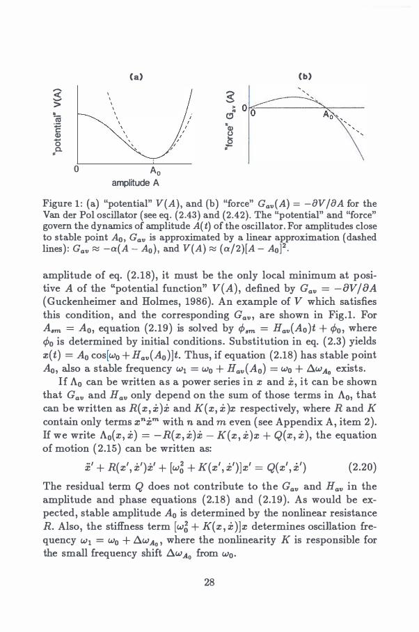
Figure 1 : (a) "potential" V(A), and (b) "force" Gav(A) = -8Vf8A for the Van der Pol oscillator (see eq. (2.43) and (2.42). The "potential" and "force" govern the dynamics of amplitude A( t) of the oscillator. For amplitudes close to stable point A0, Gav is approximated by a linear approximation (dashed lines) : Gav � -a(A - Ao), and V(A) � (af2)[A - Ao]2 •

amplitude of eq. (2.18), it must be the only local minimum at positive A of the "potential function" V(A) , defined by Gav = -8V/8A (Guckenheimer and Holmes, 1986). An example of V which satisfies this condition, and the corresponding Gav, are shown in Fig.l. For A.m = Ao, equation (2.19) is solved by ¢sm = Hav(Ao)t + ¢o, where ¢0 is determined by initial conditions. Substitution in eq. (2.3) yields x(t) = A0 cos[w0 + Hav(A0)]t. Thus, if equation (2.18) has stable point Ao, also a stable frequency w1 = w0 + Hav(A0) = Wo + �WA0 exists.

If A0 can be written as a power series in x and i:, it can be shown that Gav and Hav only depend on the sum of those terms in A0, that can be written as R(x, :i; )x and K(x, x )x respectively, where R and K contain only terms xnxm with n and m even (see Appendix A, item 2). If we write A0(x , x) = -R(x, x)x - K(x , x)x + Q(x , x ) , the equation of motion (2.15) can be written as:

•• I + R( I . I) • I + [ 2 + K( I · I)] I - Q( I . I) X X , X X w0 X , X X - X , X (2.20)

The residual term Q does not contribute to the Gav and Hav in the amplitude and phase equations (2.18) and (2.19). As would be expected, stable amplitude A0 is determined by the nonlinear resistance R. Also, the stiffness term [w� + K(x , :i; )]x determines oscillation frequency w1 = w0 + �w Ao , where the nonlinearity K is responsible for the small frequency shift �WA0 from Wo.

28

The fluctuating functions G1 and H1 in the complete differential equations (2.13) and (2.14), cause the actual amplitude A and phase ¢ of x(t) to deviate from the stationary values A6m = A0 and ¢6m = Hav(Ao)t. We define:

(2.21) (2.22)

Subtraction of equations (2.18) and (2.19) from the complete amplitude and phase equations (2.13) and (2.14) respectively, and using the Krylov-Bogoliubov approximation for G0 and H0, results in differential equations for hA and 6¢:

Gav(A) - Gav(A6m) + G1(A, ¢, t) Hav(A) - Hav(A6m) + Ht(A, ¢, t)

(2.23) (2.24)

In the following, we will replace the arguments A and ¢ of the functions G1 and H1 , by their stationary values A0 and 6.wA0 t . This is allowed if G1 and H1 cause only small fluctuations hA and h¢ (Stratonovich, 1963b ) . 2

Since we assumed G1 and H1 to cause only small deviations from amplitude A0 and frequency w0 + b..w Ao , we can use a linear approximation for H av and G av :

-a(A - A0) b..wAo + ,B(A - Ao)

(2.25) (2.26)

where a: = -dGav/dAIA=Ao > 0 (see Fig.1b), and ,8 = dHav/dA IA=Ao · Substitution of these equations in the differential equations (2.23) and (2.24) yields:

-ahA + G1 (t) ,BhA + H1 (t)

(2.27) (2.28)

for amplitude and phase deviations. We dropped the stationary amplitude and phase as arguments of G1 and H1 •

2In fact, the variation of G1 and H1 , due to variation of 8A and 8¢ must be negligible: oA X (8Gif8AIA=Ao ) � Gl(Ao, WA0t, t) , 8¢ X (8Gif8¢irJ>=AwA0t) � Gl(Ao, WA0t, t), etc.

29

These fluctuation equations describe amplitude and phase fluctuations of a large class of oscillators. In order to derive them we assumed that (1) c5A and c54> are small fluctuations, (2) there exists one stable amplitude A0, and (3) A0( :z: , :i:) can be written as a power series of :z: and :i:.

The amplitude equation (2.27) acts as a low pass filter with input G1(t) and output c5A(t). This can easily be verified by substitution of G1 = G exp( -iwt) . Then, the amplitude equation is solved by c5A(t) = (iw + a)-1G exp(-iwt) . The passband of the "filter" is given by (w2 + a2t1 and its phase response is arg( iw + a )-1 • Since this filter is linear, the rms-fluctuation c5A,.m .. is proportional to G1 ,,.m.o·

(2.29)

The proportionality constant C depends on the fraction of spectral components of G1 that falls within the passband of the hypothetical filter. Power spectral density Su(w) of c5A can be obtained by multiplying the power spectral density Sc1 ( w) of G1 by the shape ( w2 + a2)-1 of the hypothetical filter:

S ( ) _ Sc1 (w) .SA W - 2 + 2 w a

(2.30)

The rms-fluctuation c5A,.m.o (and thus the constant C in eq. (2.29)) can be obtained by calculating the area covered by Su (Stratonovich, 1963a/b):

(2.31)

Instantaneous frequency of :z:(t) = A cos cp is defined by w1 = cP (Papoulis, 1984) . Using «P = w0t + 4>(t) (see eq. (2.3)), we find: w1 = Wo + Hav( t) = Wo + l:l.wAo + s¢. Frequency fluctuation causes the power spectral density Sz( w ) to spread out over a certain frequency interval around wl = Wo + l:l.wAo · If ( 1 ) c5wi(t) = sJ>

is lowpass Gaussian noise, with cutoff frequency l:l.wwn and (2) l:l.wwr > WJ,,.m .. , 3 then (Middleton,1960): (a) Sz(w) is approximately a Lorenzian peak, with center

3In words: bandwidth of the frequency modulating signal is larger than instantaneous frequency modulation of the signal, that is modulated

30

frequency w1 , and (b) full width at half maximum (FWHM) of this peak is approximately given by:

(2.32)

where, frequency rms-fluctuation wr,rm• equals h¢rm• ' and follows from equation (2.28).

The fluctuating functions G1 and H1 in the amplitude and phase equations (2.27) and (2.28) both depend on A1 • Therefore, amplitude and frequency fluctuations are related. We will illustrate this relation with three specific examples, using the tools presented by eq. (2.30) , (2.31 ) , and (2.32) :

Linear stiffness oscillator, driven by white Gaussian noise For an oscillator with linear stiffness, the stiffness term in equation

of motion (2.20) (and thus in the complete equation of motion (2. 1 ) ) reduces to w�x , i.e. K(x, :i;) = 0. Consequently Hav = 0 (Appendix A, item 1 and 2) , f3 = 0, and �WA0 = 0 (eq. (2.26)) . The oscillator has stable frequency w0• The noise excitations of the oscillator are written as:

A1(z, x , t) = 17(t) (2.33)

where 77(t) is Gaussian noise with constant power spectral density S'1. The fluctuating functions in the amplitude and phase equations (2.27) and (2.28) become:

17( t) . -- sm(w0t + ¢0) Wo 17(t)

--A

cos(wot + ¢o) Wo o

(2.34)

(2.35)

with power spectral density SG1 = �S'1/w� , and SH1 = �S'1/(A�w�) . The resulting fluctuation equations (2.27) and (2.28) for amplitude and phase, have been extensively treated by Stratonovich (1963a) . We will briefly review his results.

Phase will display a diffusional behaviour: the square of the rmsvalue of phase shift �¢ = 6¢(t + T) - 6¢(t), which occurs during T

31

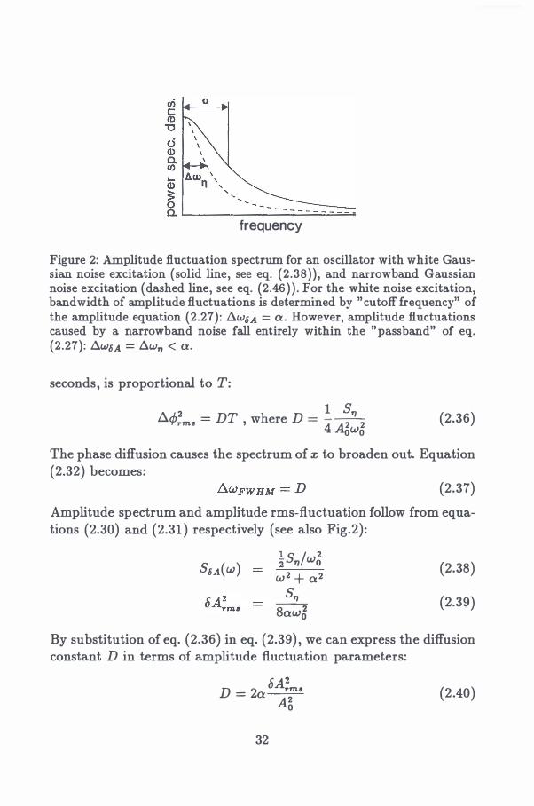
frequency Figure 2: Amplitude fluctuation spectrum for an oscillator with white Gaussian noise excitation (solid line, see eq. (2.38)), and narrowband Gaussian noise excitation (dashed line, see eq. (2.46)) . For the white noise excitation, bandwidth of amplitude fluctuations is determined by "cutoff frequency" of the amplitude equation (2.27): Awu = a. However, amplitude fluctuations caused by a narrowband noise fall entirely within the "passband" of eq. (2.27): Awu = t::.w,., < a.

seconds, is proportional to T:

2 1 s,., l::ic/Jrma = DT , where D = - A2 2 4 oWo

(2.36) The phase diffusion causes the spectrum of x to broaden out. Equation (2.32) becomes:

(2.37) Amplitude spectrum and amplitude rms-fluctuation follow from equations (2.30) and (2.31 ) respectively (see also Fig.2):

Su(w) �S,.,/w5 w2 + a2

s,., Saw�

(2.38) (2.39)

By substitution of eq. (2.36) in eq. (2.39) , we can express the diffusion constant D in terms of amplitude fluctuation parameters:

D- 6A;m• - 2a

A2 0

32

(2.40)

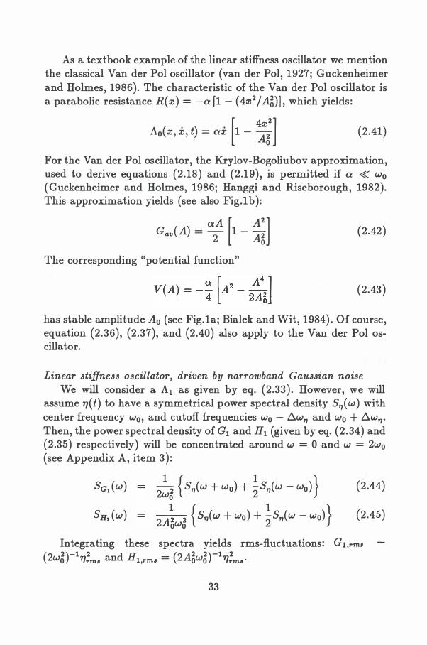
As a textbook example of the linear stiffness oscillator we mention the classical Van der Pol oscillator (van der Pol, 1927; Guckenheimer and Holmes, 1986). The characteristic of the Van der Pol oscillator is a parabolic resistance R( x) = -a [1 - ( 4:z:2 /A�) J , which yields:

A0(:e, x, t) = ax [1 - �;] (2.41)

For the Van der Pol oscillator, the Krylov-Bogoliubov approximation, used to derive equations (2.18) and (2.19), is permitted if a � w0 (Guckenheimer and Holmes, 1986; Hanggi and Riseborough, 1982). This approximation yields (see also Fig.1 b):

aA [ A2 ] G av ( A) = 2 1 -

A5 (2.42)

The corresponding "potential function"

(2.43)

has stable amplitude A0 (see Fig.1a; Bialek and Wit, 1984) . Of course, equation (2.36), (2.37), and (2.40) also apply to the Van der Pol oscillator.

Linear stiffness oscillator, driven by narrowband Gaussian noise We will consider a A1 as given by eq. (2.33) . However, we will

assume 17(t) to have a symmetrical power spectral density S71(w) with center frequency w0, and cutoff frequencies w0 - D..w71 and w0 + D..w71• Then, the power spectral density of G1 and H1 (given by eq. (2 .34) and (2.35) respectively) will be concentrated around w = 0 and w = 2w0 (see Appendix A, item 3) :

SG1 (w) � {s71(w + w0) + �S71(w - w0)} (2.44) 2w0 2

SH1 (w) A� 2 {s77(w + w0) + �S71(w - w0)} (2.45)

2 0w0 2

Integrating these spectra yields rms-fluctuations: G1 ,rm• -(2w�)-1

TJ;m• and Hl,rm• = (2A�w�)-1TJ;m. ·

33

Consider a very narrow noiseband .6wfl � a � w0• Then the first term in eq. (2.44) completely falls within the passband of the hypothetical filter, described by eq. (2.27). The second term is completely filtered out. Substitution of eq. (2.44) in (2.30) yields :

1 Su(w) = 2 2 Sfl(w + w0) 2a w0 (2.46)

Bandwidth of amplitude fluctuations will not be determined by cutoff frequency a of the "filter" , but is equal to cutoff frequency .6wfl of Sfl(w + w0) (see Fig.2). amplitude rms-fluctuation is given by:

(2.47)

Since H1 contains a prominent low frequency component, instantaneous frequency w1(t) = w0 + 6¢ will show slow fluctuations, with bandwidth .6wfl. Frequency rms-fluctuations follow straight forward from eq. (2.28) (recall {3 = 0):

(2.48)

Eliminating 77,.m• from eq. (2.47) and (2.48) yields a relation beween amplitude and frequency fluctuations:

(2.49)

This equation will still be approximately valid if .6wfl ;:S a, i.e. if the bandwidth of the noise is approximately equal to, or smaller than, bandwidth a of the amplitude equation (2.27). Then, since spectral components of G1 at frequencies of the order of a are slightly attenuated, '='-signs in equations (2 .46) , (2.47) and (2.49) should be replaced by ' ;:S '.

Nonlinear stiffness oscillator If stiffness is nonlinear, K(:z:, :i:) =/=- 0 . The stationary frequency of

the oscillator we will be shifted from w0 by an amount .6w Ao . As has been stated before, nonlinear stiffness does not affect the amplitude

34

equation (2.27) . All results for amplitude fluctuations, derived so far, remain unchanged. However, the nonlinear stiffness results in an extra term (36A in the phase equation (2.28). This extra fluctuating term is responsible for extra fluctuation of frequency of the oscillator. Also, it causes frequency fluctuation to be directly related to amplitude fluctuation. For example, if (3 > 0 ( "hard spring condition", see Stoker, 1950) an amplitude increase 6A results in an increase of instantaneous frequency: w1 = (36A + . . . . If (36A is the dominating term in the righthand side of the phase equation (2.28), comparison of 6Arm• and WJ,rm• gives an estimate of (3:

(2.50)

A textbook example of a nonlinear stiffness oscillator is the Duffing oscillator (Duffing, 1918; Guckenheimer and Holmes, 1986) . The characteristic of the Duffing oscillator is a quadratic nonlinear stiffness K(x), which we will write as:

:z:2 K(x) = w�b-2 Ao

(2.51)

Using Krylov-Bogoliubov approximation yields Hav(A) = �bw0A2 /A� (Nayfeh and Mook, 1979). Thus, stationary frequency is shifted from Wo by an amount �WA0 = Hav(Ao) = �bwo , and (3 = dHav/dA IA=Ao =

�bw0/A0 • Stationary amplitude A0 in these expressions, depends on the resistance term R(x, x ) . For an oscillator with a Duffing stiffness term, parameter b follows from equation (2.50) :

b = � WJ,rma/Wo 3 6Arma/Ao


(2.52)

Spontaneous otoacoustic emission (SOAE) recordings were performed in 8 human and 2 frog ( Rana esculenta) ears. Emissions were measured with a sensitive microphone (Wit et al., 1981 ) . The microphone signal was stored on video tape (Sony SL-C30E video recorder) after pulse code modulation (Sony PCM-Fl ). Typically, recordings lasted 80 s.

35

All investigated human and frog ears had one spontaneous otoacoustic emission, which was at least 10 dB stronger than all other emissions (if present) in the same ear. For further analysis we focused on this strong emission.

The microphone signals were the sum of the otoacoustic emission signal and noise from the measuring equipment . In addition to recordings of emissions, a recording was made of a comparison signal, being the sum of a stable sinusoid (generated by a Wavetek 178 signal synthesizer) and broadband Gaussian noise. Signal to noise ratio of the comparison signal was approximately equal to that of emission recordings. All analysis procedures described below were also performed on this comparison signal, in order to investigate the effect of background noise on the results.

Recorded emission signals were Fourier transformed, with a Unigon 4512 FFT analyzer, using a zoom procedure. All FFT applications described in this work were preceded by multiplication of the time signal by a Hanning weighting function. The resulting spectra were least squares fitted with a curve S:z:(B, fl l !::if, C l f) = B/[(f - !1 )2 + i(!::ifFWHM)2] + C, i.e. the sum of a Lorenz curve and a constant C. The constant C reflects the contribution of the microphone noise to the spectrum. The fit yields frequency f1 = wif27r and spectral width !:l.fFWHM = !:l.wFWHM/27r of the emission signal. 4

Amplitude fluctuations For investigation of emission amplitude fluctuations, the recorded

microphone signal was first filtered using a B&K 1623 bandpass filter, in order to reduce the influence of microphone noise. Filter center frequency was equal to the frequency of the (dominating) emission. Bandwidth of the filter was 23 % of center frequency. The envelope of the bandpass filtered signal was determined by subsequent rectification and lowpass filtering (Hsu, 1967).

The resulting envelope signal 6AENv(t) was fast Fourier transformed (Unigon 4512). An idealized representation of an envelope spectrum is given in Fig. 3. Evidently, the envelope spectra were the

4Throughout the manuscript, the letter f with or without subscript is used for cycles per second. Greek symbols, denoting frequency, refer to angular frequency. Thus, for example: wo = 211" fo

36

>--"ii) c 0,)

"t]

cj 0,) a. (/) ..... 0,) :: 0 a.

frequency

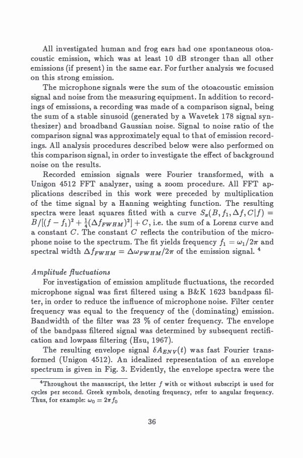
Figure 3: Schematic representation of the power spectral density of the envelope of an emission recording. The microphone signal was bandpass filtered. Center frequency of the filter was set at the frequency of an emission. The spectrum contains two contributions. The area B reflects the contribution of microphone noise, within the passband of the filter. This contribution is truncated at half filter bandwidth ( � f _3dB ) . Area A reflects the amplitude fluctuations of the emission signal. For the comparison signal, consisting of a sinusoid with stable amplitude to which noise is added, only contribution B will be found.

sum of two components: (1) Contribution B : present for both the recorded comparison and emission signals, and (2) Contribution A: present only for the recorded emission signals. Apparently, the envelope is the sum of two components: B is a contribution of background microphone noise, and A of amplitude fluctuation of the emission signal. Envelope spectra were fitted with a curve SENv(b, !),.Ju, C lf ) = b/ [P+ (f),.fu)2] +C . The Lorenzian term in SENV reflects contribution A, and the constant C reflects contribution B .

In order to determine the relative rms-fluctuation 6Arm6/ Ao of an emission signal (contribution A) , we first determined the rms-value 6AENV,rm6 of the envelope h'AENv(t) (contribution A+B ) . A DATALAB 4000 system was used to determine the probability distribution of h'AENV· The width of this distribution is proportional to 6AENV,rm6 · To calibrate this width, the probability distribution of the envelope of a signal with known amplitude modulation was determined. This signal was generated by a Wavetek 178 waveform synthesizer in AMmode, with the AM-input connected to a low pass Gaussian noise

37

(cutoff frequency 50 Hz) from a HP 3 722A noise generator. Finally, the relative amplitude rms-fluctuation of the emission was

calculated using:

(hArm• ) 2 =

Area A (hAENV,rm•) 2 (2.53)

A0 Area A+B A0

From the fit S ENv(i) (see above) we determined Area A ('rr/2) .b.l!:l.fu , and Area A+B was calculated by integrating the amplitude spectrum.

Frequency fluctuations In order to investigate frequency fluctuations of emissions signals,

the phase relation between an emission signal and a reference signal with frequency !ref close to the emission frequency was determined. First, a B&K 2020 heterodyne bandpass filter was used to filter the recorded microphone signal. Center frequency of the filter was set at the frequency of the emission under investigation. Bandwidth was 100 Hz. A HP 5326A timer was used to measure the time 6.1';, between the i-th positive-going zero-crossing of the reference signal and the subsequent positive-going zero-crossing of the emission signal. The phase of the emission with respect to the reference is given by </>( i) = 27r frefl!:l.T;,. Successive values of 6.1';, were stored on computer disk.

The period of the emission signal is given by: Ti = ( 1/ !ref) + l!:l.Ti -6.1';,_1 • The signal T;, , or T(t), was analyzed in sections of 2048 data points, corresponding to a time window of 2048/ !ref seconds, typically 1.6 s. For each section, the average period To = (T(t)) was computed. Then we calculated the fast Fourier transform of hT( t) = T( t) - T0 for each time window. Spectra of successive time windows were added, resulting in an average spectrum of hT(t) = T(t) - T0 for the entire emission recording. This spectrum consists of a contribution from the emission, and a contribution from the background microphone noise. We fitted the spectrum to a Lorenzian curve s6T(B, l!:l.JDT, aif) =

B ![j2 + (l!:l.fT )2] + a X s6T(noi•e) ' where a X s6T(noi•e) is the contribution of the background noise. As will be shown in Appendix B , S6T(noi•e) is independent of amplitude and frequency of the emission. We determined S6T(noi•e) in a phenomenological way by fitting the spectrum of hT(t) as found for the comparison signal, to a lOth-order polynomial.

38

1 .0

>. -'Cii c: Q)

'C

g 0.5 c. en ... Q) � 0 c.

0

0

0

1 397 frequency {Hz)

1 398

Figure 4: Power spectral density of the microphone signal recorded for subject AS , zoomed in on a strong emission in the subjects ear at 1397 Hz. The solid line is a leastsquares Lorenzian fit. Spectral width l:!..fFWHM of the peak was 0.25 Hz.

From the sampled signal T(t) we calculated the rms-value: bTE+N,rm• = (�ihTj+N,rm.,i)112 , where hTE+N,rm•,i are the rmsvalues of T(t) of successive time windows of 2048/ !ref seconds. Like hAENV,rm•' hTE+N,rm• is the sum of a contribution from the emission signal (E) and the microphone noise (N). We used the spectrum S6T(i), to calculate the rms-fluctuation hTrm• of the emission period, analogous to the procedure illustrated in Fig. 3.

Results

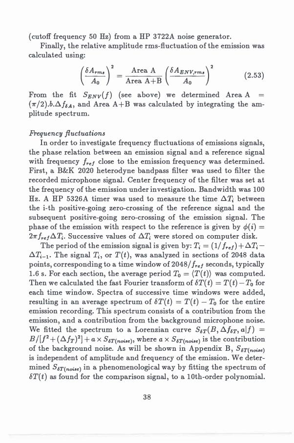
As an example Fig. 4 shows the power spectrum of the microphone signal, as recorded in subject AS, zoomed in on the emission at 1397 Hz. The full width at half maximum llfFWHM of this spectrum is 0.25 Hz. For all human subjects, llfFWHM ranged from 0.25 to 1 .50 Hz. For two frog emissions the spectral width was 2.9 and 8.0 Hz respectively.

Fig. 5 shows the power spectrum of the envelope signal for subject WK. The width at half maximum llfu of the emission contribu-

39

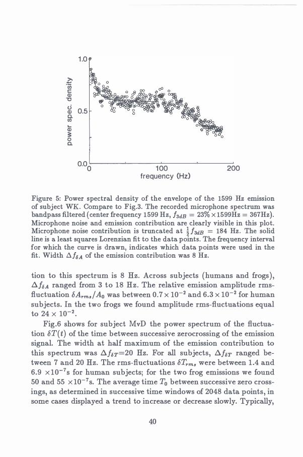
>. :t:: en c (J)

"C c.:i (J) 0. en .... (J) 3: 0 0.

1 .0

0.5

0.00 1 00 frequency (Hz)

200

Figure 5: Power spectral density of the envelope of the 1599 Hz emission of subject WK. Compare to Fig.3. The recorded microphone spectrum was bandpass filtered (center frequency 1599 Hz, fadB = 23% X 1599Hz = 367Hz) . Microphone noise and emission contribution are clearly visible in this plot. Microphone noise contribution is truncated at l fadB = 184 Hz. The solid line is a least squares Lorenzian fit to the data points. The frequency interval for which the curve is drawn, indicates which data points were used in the fit . Width 11fu of the emission contribution was 8 Hz.

tion to this spectrum is 8 Hz. Across subjects (humans and frogs) , !:l.fu ranged from 3 to 18 Hz. The relative emission amplitude rmsfluctuation 8Arm,/A0 was between 0.7 X 10-2 and 6.3 X 10-2 for human subjects. In the two frogs we found amplitude rms-fluctuations equal to 24 x 10-2 •

Fig.6 shows for subject MvD the power spectrum of the fluctuation 8T(t) of the time between successive zerocrossing of the emission signal. The width at half maximum of the emission contribution to this spectrum was !:l.f6T=20 Hz. For all subjects, !:l.f6T ranged between 7 and 20 Hz. The rms-fluctuations 8Trm" were between 1 .4 and 6.9 x 10-7s for human subjects; for the two frog emissions we found 50 and 55 x 10-7 s. The average time T0 between successive zero crossings, as determined in successive time windows of 2048 data points, in some cases displayed a trend to increase or decrease slowly. Typically,

40

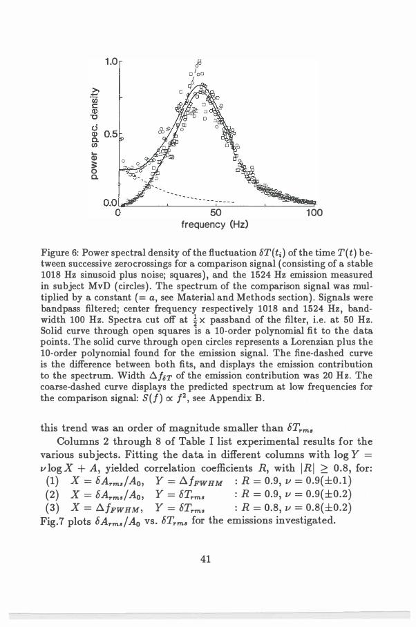
.... Q) 3: 0 c.

1 .0

50 frequency (Hz)

1 00

Figure 6: Power spectral density of the fluctuation 6T(ti) of the time T(t) between successive zero crossings for a comparison signal (consisting of a stable 1018 Hz sinusoid plus noise; squares) , and the 1524 Hz emission measured in subject MvD (circles) . The spectrum of the comparison signal was multiplied by a constant ( = a, see Material and Methods section) . Signals were bandpass filtered; center frequency respectively 1018 and 1524 Hz, bandwidth 100 Hz. Spectra cut off at � X passband of the filter, i.e. at 50 Hz. Solid curve through open squares is a 10-order polynomial fit to the data points. The solid curve through open circles represents a Lorenzian plus the 10-order polynomial found for the emission signal. The fine-dashed curve is the difference between both fits, and displays the emission contribution to the spectrum. Width 6.f5T of the emission contribution was 20 Hz. The coarse-dashed curve displays the predicted spectrum at low frequencies for the comparison signal: S(f) ex: P, see Appendix B.

this trend was an order of magnitude smaller than 6Trm11 Columns 2 through 8 of Table I list experimental results for the

various subjects. Fitting the data in different columns with log Y = v log X + A, yielded correlation coefficients R, with IR I 2:: 0.8, for: (1) X = 6Arm11/Ao, Y = D.fFWHM : R = 0.9, Z1 = 0.9(±0.1 ) (2) X = 6Arm11/Ao , Y = 6Trm11 : R = 0.9, Z1 = 0.9(±0.2) (3) X = D.JFWHM, Y = 6Trm11 : R = 0.8, Z1 = 0.8(±0.2)

Fig.7 plots 6Arma/A0 vs. 6Trma for the emissions investigated.

41

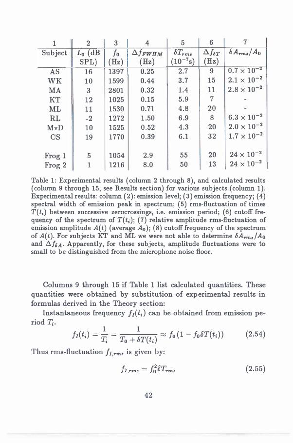
1 2 3 4 5 6 7 Subject L0 (dB fo _6.fFWHM STrma .6.f6T SArm•/Ao

SPL) (Hz) (Hz) (lo-7s) (Hz) AS 16 1397 0.25 2.7 9 0.7 X 10 2 WK 10 1599 0.44 3.7 15 2.1 X 10-2 MA 3 2801 0 .32 1 .4 11 2 .8 X 10-2 KT 12 1025 0.15 5.9 7 -ML 11 1530 0.71 4.8 20 -RL -2 1272 1 .50 6 .9 8 6.3 X 10-2

MvD 10 1525 0 .52 4.3 20 2.0 X 10-2 cs 19 1770 0.39 6.1 32 1 .7 X 10-2

Frog 1 5 1054 2.9 55 20 24 X 10-2 Frog 2 1 1216 8.0 50 13 24 X 10-2

Table 1 : Experimental results (column 2 through 8), and calculated results (column 9 through 15, see Results section) for various subjects (column 1 ) . Experimental results: column {2 ) : emission level; ( 3 ) emission frequency; (4) spectral width of emission peak in spectrum; (5) rms-fluctuation of times T(ti) between successive zerocrossings, i.e. emission period; (6) cutoff frequency of the spectrum of T(ti) i (7) relative amplitude rms-fluctuation of emission amplitude A(t) (average A0) ; (8) cutoff frequency of the spectrum of A(t). For subjects KT and ML we were not able to determine 5Arma/Ao and !:if6A· Apparently, for these subjects, amplitude fluctuations were to small to be distinguished from the microphone noise floor.

Columns 9 through 15 if Table 1 list calculated quantities. These quantities were obtained by substitution of experimental results in formulas derived in the Theory section:

Instantaneous frequency fr(ti ) can be obtained from emission period Ti.

1 1 fi(ti) = Ti = To + ST(ti ) � fo (1 - foST(ti ) )

Thus rms-fluctuation Jr,rm• is given by:

42

(2.54)

(2.55)

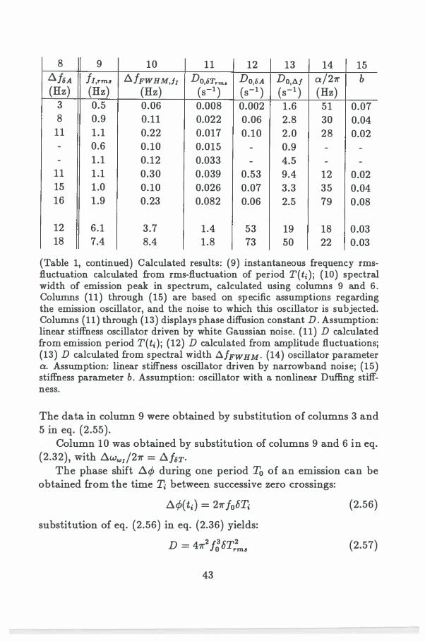
8 9 10 11 12 13 14 15 tl.fu fi,rmlt /l.fFWHM,fr Do,6T.-m• Do,OA Do,at ex. /27r b (Hz) (Hz) (Hz) (s-1 ) (s-1 ) (s-1 ) (Hz)

3 0.5 0.06 0.008 0.002 1 .6 51 0.07 8 0.9 0.11 0.022 0.06 2.8 30 0.04 11 1 .1 0.22 0.017 0.10 2.0 28 0.02 - 0.6 0.10 0.015 - 0.9 - -- 1 .1 0.12 0.033 - 4.5 - -

11 1 .1 0.30 0.039 0.53 9.4 12 0.02 15 1 .0 0.10 0.026 0.07 3.3 35 0.04 16 1 .9 0.23 0.082 0.06 2.5 79 0.08

12 6.1 3.7 1.4 53 19 18 0 .03 18 7.4 8.4 1.8 73 50 22 0.03

(Table 1, continued) Calculated results: (9) instantaneous frequency rmsfluctuation calculated from rms-fluctuation of period T(ti) i (10) spectral width of emission peak in spectrum, calculated using columns 9 and 6 . Columns (11) through ( 15) are based on specific assumptions regarding the emission oscillator, and the noise to which this oscillator is subjected. Columns (11) through (13) displays phase diffusion constant D . Assumption: linear stiffness oscillator driven by white Gaussian noise. (11) D calculated from emission period T(ti) i (12) D calculated from amplitude fluctuations; (13) D calculated from spectral width tifFWHM· (14) oscillator parameter ex.. Assumption: linear stiffness oscillator driven by narrowband noise; (15) stiffness parameter b. Assumption: oscillator with a nonlinear Duffing stiffness.

The data in column 9 were obtained by substitution of columns 3 and 5 in eq. (2.55).

Column 10 was obtained by substitution of columns 9 and 6 in eq. (2.32), with tl.ww1/27r = tl.f6T·

The phase shift fl.¢ during one period T0 of an emission can be obtained from the time 7i between successive zero crossings:

fl.¢( ti) = 27r fo87i

substitution of eq. (2.56) in eq. (2.36) yields:

D = 47r2 jg 8Tr2ma

43

(2.56)

(2.57)

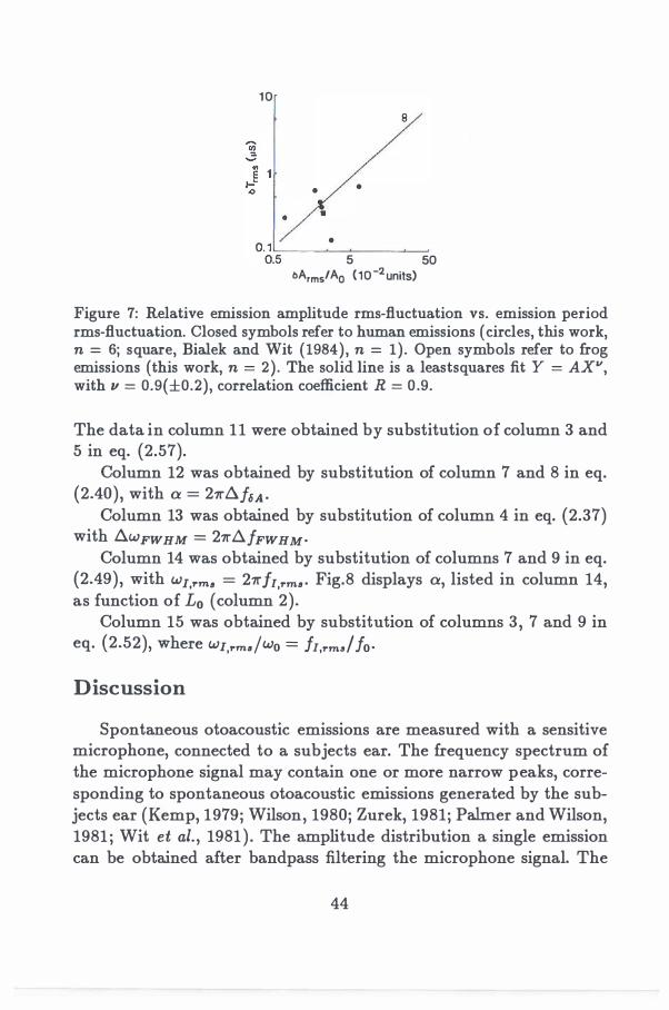
10

•

•

•

8

•

5 50 bArm5/A0 (10-2units)

Figure 7: Relative emission amplitude rms-fluctuation vs. emission period rms-fluctuation. Closed symbols refer to human emissions (circles, this work, n = 6; square, Bialek and Wit (1984), n = 1) . Open symbols refer to frog emissions (this work, n = 2) . The solid line is a leastsquares fit Y = AX", with 11 = 0.9(±0.2), correlation coefficient R = 0 .9.

The data in column 11 were obtained by substitution of column 3 and 5 in eq. (2.57).

Column 12 was obtained by substitution of column 7 and 8 in eq. (2.40), with a = 27rl::ifliA·

Column 13 was obtained by substitution of column 4 in eq. (2.37) with f:::t.wFWHM = 27r/::ifFWHM·

Column 14 was obtained by substitution of columns 7 and 9 in eq. (2.49), with WJ,rma = 27rfi,rma · Fig.8 displays a, listed in column 14, as function of L0 (column 2).

Column 15 was obtained by substitution of columns 3, 7 and 9 in eq. (2.52), Where WJ,rTTu/Wo = h,rmsl fo·

Discussion

Spontaneous otoacoustic emissions are measured with a sensitive microphone, connected to a subjects ear. The frequency spectrum of the microphone signal may contain one or more narrow peaks, corresponding to spontaneous otoacoustic emissions generated by the subjects ear (Kemp, 1979; Wilson, 1980; Zurek, 1981; Palmer and Wilson, 1981 ; Wit et al. , 1981 ) . The amplitude distribution a single emission can be obtained after bandpass filtering the microphone signal. The

44

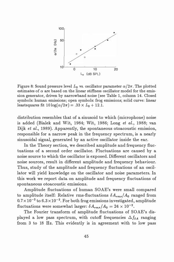
100

'N 50 � c

C\J ...... c 0

•

1 0 0

•

0

Lo

•

1 0 (dB SPL)

•

•

20

Figure 8: Sound pressure level L0 vs. oscillator parameter a.j21r. The plotted estimates of a are based on the linear stiffness oscillator model for the emission generator, driven by narrowband noise (see Table 1 , column 14. Closed symbols: human emissions; open symbols: frog emissions; solid curve: linear leastsquares fit 10 log( a./27r) = .33 X L0 + 12.1 .

distribution resembles that of a sinusoid to which (microphone) noise is added (Bialek and Wit, 1984; Wit, 1986; Long et al. , 1988; van Dijk et al., 1989). Apparently, the spontaneous otoacoustic emission, responsible for a narrow peak in the frequency spectrum, is a nearly sinusoidal signal, generated by an active oscillator inside the ear.

In the Theory section, we described amplitude and frequency fluctuations of a second order oscillator. Fluctuations are caused by a noise source to which the oscillator is exposed. Different oscillators and noise sources, result in different amplitude and frequency behaviour. Thus, study of the amplitude and frequency fluctuations of an oscillator will yield knowledge on the oscillator and noise parameters. In this work we report data on amplitude and frequency fluctuations of spontaneous otoacoustic emissions.

Amplitude fluctuations of human SOAE's were small compared to amplitude itself: Relative rms-fluctuations hArm•/ A0 ranged from 0. 7 x 10-2 to 6 .3 x 10-2• For both frog emissions investigated, amplitude fluctuations were somewhat larger: hArma/A0 = 24 X 10-2 •

The Fourier transform of amplitude fluctuations of SOAE's displayed a low pass spectrum, with cutoff frequencies t:l.fu ranging from 3 to 18 Hz. This evidently is in agreement with to low pass

45

characteristic of the amplitude fluctuation equation (2.27) . However, from these experiments it is impossible to decide whether l:ifu can be equated the cutoff frequency a/27r of the amplitude equation, or is merely the cutoff frequency of the fluctuation function G1 • The latter could fall well within the passband a of equation (2.27).

The parameter a also determines the amplitude relaxation behaviour of the oscillator. The average solution of equation (2.27) with initial condition A(t=O) = hA0 is: (hA(t)} = hA0 exp( -at). Defining relaxation time Trel as the time needed to relax to hA(t) = e-1hA0,

. ld -l Jle S Trel = a . Schloth and Zwicker (1983) studied amplitude relaxation of

SOAE's after suppression. They used a suppressing tone, switched on for 60 ms, to change the amplitude of a spontaneous otoacoustic emission by 6 dB. After switching off the suppressing tone, they found the emission amplitude to relax to its unsuppressed value with a median relaxation time of 13.2 ms. This relaxation time would corresponds to a cutoff frequency a/27r = 12.1 Hz of the amplitude equation (2.27). We found the cutoff frequency of amplitude spectra to be l:ifu = 12(±4) Hz on average. So, the measured cutoff frequency !:ihA of amplitude fluctuations, and cutoff frequency {27rTrez)-1 predicted from relaxation experiment of Schloth and Zwicker (1983) , are comparable. This suggests that the measured cutoff frequency l:ifu of amplitude fluctuations corresponds to the cutoff frequency a of the lowpass filter described by eq. (2.27) (i.e. l:ifu = aj21r), instead of being the cutoff frequency of fluctuation function G1 7 falling within the passband a.

However, this conclusion is based on the assumption that (1 ) suppression of an SOAE does not change parameters of the emission generator, and (2) conditions used for deriving the amplitude equation (2.27) are valid. The first assumption can not be easily verified, but the second is evidently violated. One of the conditions used to derive the amplitude equation was: !hAl � A0• This condition is clearly not satisfied for a 6 dB level suppression, which corresponds to hA = -�A0• Consider for example amplitude relaxation as described by the potential function V(A) of the Van der Pol oscillator (eq. (2.43) and Fig.1a, solid curve) : The relation a = Tr�J (see above) is based on the assumption that the dashed curve in Fig.1a is a good approximation

46

for V(A). As is clear from Fig.1a, this is not the case for h"A = -�Ao (i.e. A = �A0). A straightforward computer simulation, using �he po-tential V(A) corresponding to the solid line in Fig.1a (see eq(2.43)), yielded that relaxation from 6 dB suppression takes a relaxation time r,.el approximately twice as large as a-1 . Thus, for the Van der Pol oscillator, a = r,.:f underestimates a by a factor 2.

If we assume spontaneous emissions to be generated by a Van der Pol oscillator, then the median relaxation time r,.el = 13.2ms, determined by Schloth and Zwicker (1983) corresponds to a cutoff frequency of the amplitude equation (2.27) of about aj21r :;:::j 2 x (27rr,.el)-1

= 24.1Hz. This is larger than all cutoff frequencies 1:1/u that we determined from amplitude fluctuation spectra (see Table 1, column 8). So possibly 1:1/u is not determined by a, but by the cutoff frequency of the fluctuating function G1• Further experiments are needed to clarify the relation between 1:1/u and a (see Conclusion section).

Frequency fluctuations were small compared to frequency of an emission. Width !::J.fFWHM of the power spectrum of the emission signal, ranged from 0.25 to 1.5 Hz for human subjects. In both frogs we found I::J.fFWHM to be 2.9 and 8.0 Hz. Van Dijk et al. (1989), who investigated 29 frogs Rana esculenta, found an average width !::J.fFWHM of 38 Hz. This is still only a few percent of emission frequency.

Instantaneous frequency w1(ti ) can be obtained from the time T( ti ) between successive zero-crossings of the emission recording (see eq. (2.54)). Since fluctuation h"w1(ti) = wr(ti) - w0 of instantaneous frequency is proportional to fluctuation of emission period 6T(ti ) = T(ti) - T0, the power spectral densities of h"wr(ti) and 6T(ti ) are proportional to each other. Spectra of 6T displayed a low pass shape, similar to amplitude fluctuation spectra. Width !::J.f6T of these spectra ranged from 7 to 32 Hz, with average 16(±7) Hz. Thus, instantaneous frequency of an emission fluctuates slow compared to its own frequency.

Equation (2.32) gives the relation between instantaneous frequency fluctuation wr(t) and the width !::J.fFWHM of a signal with low pass frequency fluctuation. Using this equation, we estimated I::J.fFWHM from /r,,.m• and !::J.hT· For human emissions, the result (Table 1, column 10) is systematically smaller then the actual !::J.fFWHM

47

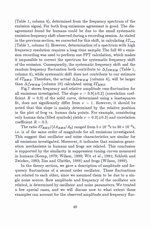
(Table 1 , column 4), determined from the frequency spectrum of the emission signal. For both frog emissions agreement is good. The disagreement found for humans could be due to the small systematic emission frequency shift observed during a recording session. As stated in the previous section, we corrected for this shift , in calculating hTrm• (Table 1 , column 5). However, determination of a spectrum with high frequency resolution requires a long time sample: The full 80 s emission recording was used to perform one FFT calculation, which makes it impossible to correct the spectrum for systematic frequency shift of the emission. Consequently, the systematic frequency shift and the random frequency fluctuation both contribute to tl.fFWHM (Table 1, column 4), while systematic shift does not contribute to our estimate of hTRMS· Therefore, the actual tl.fFWHM (column 4), will be larger than tl.fFWHM (column 10) calculated using hTRMS·

Fig. 7 shows frequency and relative amplitude rms-fluctuation for all emissions investigated. The slope v = 0.9(±0.2) (correlation coefficient R = 0.9) of the solid curve, determined using a least squares fit , does not significantly differ from v = 1 . However, it should be noted that this slope is mainly determined by the relative position in the plot of frog vs. human data points . For example, considering only human data (filled symbols) yields v = 0 .2(±0.3) and correlation coefficient R = 0.3.

The ratio hTRMs/(hARMs/A0) ranged from 5 x 10-6s to 38 x 10-6s, i.e. is of the same order of magnitude for all emissions investigated. This suggest that oscillator and noise characteristics are similar for all emissions investigated. Moreover, it indicates that emission generation mechanisms in humans and frogs are related. This conclusion is supported by the similarity in suppression tuning curves measured in humans (Kemp, 1979; Wilson, 1980; Wit et al. , 1981; Schloth and Zwicker, 1983; Ziss and Glattke, 1988) and frogs (Wilson, 1989).

In the theory section, we gave a description of amplitude and frequency fluctuations of a second order oscillator. These fluctuations are related to each other, since we assumed them to be due to a single noise source. How amplitude and frequency of the oscillator are related, is determined by oscillator and noise parameters. We treated a few special cases, and we will discuss now to what extent these examples can account for the observed amplitude and frequency flue-

48

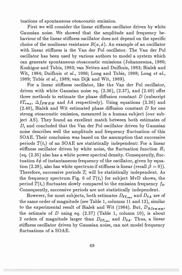
tuations of spontaneous otoacoustic emission. First we will consider the linear stiffness oscillator driven by white

Gaussian noise. We showed that the amplitude and frequency behaviour of the linear stiffness oscillator does not depend on the specific choice of the nonlinear resistance R(x, x ) . An example of an oscillator with linear stiffness is the Van der Pol oscillator. The Van der Pol oscillator has been used by various authors to model a system which can generate spontaneous otoacoustic emissions (Johannesma, 1980; Koshigoe and Tubis, 1983; van Netten and Duifhuis, 1983; Bialek and Wit , 1984; Duifhuis et al. , 1986; Long and Tubis, 1988; Long et al. , 1989; Tubis et al., 1989; van Dijk and Wit , 1989).

For a linear stiffness oscillator, like the Van der Pol oscillator, driven with white Gaussian noise eq. (2.36), (2.37), and (2.40) offer three methods to estimate the phase diffusion constant D (subscript hT,.m. , l:l.fFWHM and hA respectively) . Using equations (2.36) and (2.40) , Bialek and Wit estimated phase diffusion constant D for one strong otoacoustic emission, measured in a human subject (our subject AS). They found an excellent match between both estimates of D, and concluded that the Van der Pol oscillator driven by Gaussian noise describes well the amplitude and frequency fluctuation of this SOAE. Their conclusion was based on the assumption that successive periods T(ti) of an SOAE are statistically independent : For a linear stiffness oscillator driven by white noise, the fluctuation function H1 ( eq. (2.35) also has a white power spectral density. Consequently, fluctuation h¢ of instantaneous frequency of the oscillator, given by equation (2.28) , also has white spectrum if stiffness is linear (recall f3 = 0)) . Therefore, successive periods Ti will be statistically independent. As the frequency spectrum Fig. 6 of T(ti ) for subject MvD shows, the period T( ti ) fluctuates slowly compared to the emission frequency j0• Consequently, successive periods are not statistically independent .

However, for most subjects, both estimates D6T.,.m, and D6A are of the same order of magnitude (see Table 1 , columns 11 and 12) , similar to the experimental result of Bialek and Wit (1984) . But, Dll.fpwHM' the estimate of D using eq. (2.37) (Table 1 , column 10), is about 2 orders of magnitude larger than D6T.,.m, and Du. Thus, a linear stiffness oscillator driven by Gaussian noise, can not model frequency fluctuations of a SOAE.

49

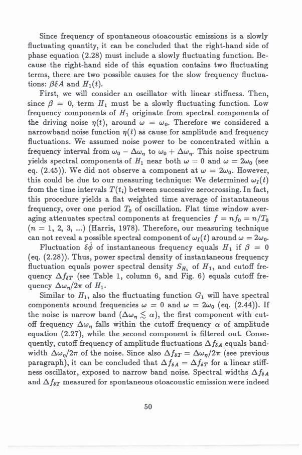
Since frequency of spontaneous otoacoustic emissions is a slowly fluctuating quantity, it can be concluded that the right-hand side of phase equation (2.28) must include a slowly fluctuating function. Because the right-hand side of this equation contains two fluctuating terms, there are two possible causes for the slow frequency fluctuations: {3SA and H1(t).

First, we will consider an oscillator with linear stiffness. Then, since {3 = 0, term H1 must be a slowly fluctuating function. Low frequency components of H1 originate from spectral components of the driving noise 77(t ) , around w = w0• Therefore we considered a narrowband noise function TJ(t) as cause for amplitude and frequency fluctuations. We assumed noise power to be concentrated within a frequency interval from w0 - .D.w11 to w0 + .D.w11• This noise spectrum yields spectral components of H1 near both w = 0 and w = 2w0 (see eq. (2.45)) . We did not observe a component at w = 2w0 • However, this could be due to our measuring technique: We determined w1(t) from the time intervals T(ti) between successive zerocrossing. In fact, this procedure yields a flat weighted time average of instantaneous frequency, over one period T0 of oscillation. Flat time window averaging attenuates spectral components at frequencies f = n/0 = n/T0 (n = 1, 2, 3, . . . ) (Harris, 1978). Therefore, our measuring technique can not reveal a possible spectral component of w1(t) around w = 2w0•

Fluctuation b� of instantaneous frequency equals H1 if {3 = 0 ( eq. (2.28)) . Thus, power spectral density of instantaneous frequency fluctuation equals power spectral density SH1 of H1 , and cutoff frequency .D.hT (see Table 1 , column 6, and Fig. 6) equals cutoff frequency .D.w11/27r of H1 •

Similar to H1 , also the fluctuating function G1 will have spectral components around frequencies w = 0 and w = 2w0 ( eq. (2.44)) . If the noise is narrow band (.D.w11 ;S a ) , the first component with cutoff frequency .D.w11 falls within the cutoff frequency a of amplitude equation (2.27), while the second component is filtered out. Consequently, cutoff frequency of amplitude fluctuations .D.fu equals bandwidth .D.w11/27r of the noise. Since also .D.foT = .D.w,.,j27r (see previous paragraph) , it can be concluded that .D.fu = .D.foT for a linear stiffness oscillator, exposed to narrow band noise. Spectral widths .D.fu and .D.foT measured for spontaneous otoacoustic emission were indeed

50

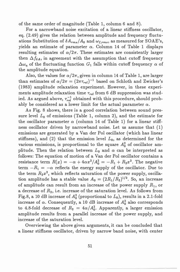
of the same order of magnitude (Table 1 , column 6 and 8). For a narrowband noise excitation of a linear stiffness oscillator,

eq. (2.49) gives the relation between amplitude and frequency fluctuations Substitution of 6Arma/A0 and WJ,rm" ' as measured for SOAE's, yields an estimate of parameter a. Column 14 of Table 1 displays resulting estimates of aj21r. These estimates are consistently larger then 6./u, in agreement with the assumption that cutoff frequency 6.w'1 of the fluctuating function G1 falls within cutoff frequency a of the amplitude equation.

Also, the values for aj21r , given in column 14 of Table 1 , are larger than estimates of aj21r = (21rTrez }-1 based on Schloth and Zwicker's (1983) amplitude relaxation experiment. However, in these experiments amplitude relaxation time Trel from 6 dB suppression was studied. As argued above, rr�t obtained with this procedure, should probably be considered as a lower limit for the actual parameter a.

As Fig. 8 shows, there is a good correlation between sound pressure level L0 of emissions (Table 1 , column 2), and the estimate for the oscillator parameter a (column 14 of Table 1) for a linear stiffness oscillator driven by narrowband noise. Let us assume that ( 1 ) emissions are generated by a Van der Pol oscillator (which has linear stiffness), and (2) that the emission level L0, as determined for the various emissions, is proportional to the square A� of oscillator amplitude. Then the relation between L0 and a can be interpreted as follows: The equation of motion of a Van der Pol oscillator contains a resistance term R(:z:) = -a + 4a:z:2/A� = -R1 + R2:z:2 • The negative term -R1 = -a reflects the energy supply of the oscillator. Due to the term R2:z:2, which reflects saturation of the power supply, oscillation amplitude has a stable value A0 = (2Rtf R2)112 • So, an increase of amplitude can result from an increase of the power supply R1 , or a decrease of R2, i.e. increase of the saturation level. As follows from Fig.8, a 10 dB increase of A� (proportional to L0) , results in a 2 .1-fold increase of a. Consequently, a 10 dB increase of A� also corresponds to 4.8-fold decrease of R2 = 4a/A�. Apparently, a larger emission amplitude results from a parallel increase of the power supply, and increase of the saturation level.

Overviewing the above given arguments, it can be concluded that a linear stiffness oscillator, driven by narrow band noise, with center

51

frequency w0, can possibly model amplitude and frequency fluctuations of spontaneous otoacoustic emissions.

A possible source for narrow band fluctuations TJ(t) is a slowly fluctuating power supply of the oscillator. Consider for example the Van der Pol oscillator, to which energy is supplied by the negative part of the resistance R( x) = - a + 4ax2 /A�. If we assume this negative term to be weakly fluctuating, eq. (2.41) becomes A0(x, :i: , t) = a:i: [1 + e(t) - (x2 /4A5)] , where e(t) reflects the small fluctuations of the power supply. Equation (2 .1) then contains a noisy function xe(t) = -w0A sin(w0+¢ )e(t). Since e was a slowly fluctuating low pass noise, xe(t) is a narrow band noise with center frequency Wo . Thus a slow fluctuation of power supply causes a narrowband noise excitation in the oscillator equation (2.1 ) .

As a second possible model, we consider a nonlinear stiffness oscillator. For this oscillator {3 =/= 0. Since hA(t) is slowly fluctuating, the right-hand side of phase equation (2.28) evidently contains a slowly fluctuating term, which can model slow frequency fluctuation measured for SOAE's. Notice that nonlinear stiffness always introduces slow frequency fluctuations, regardless of the power spectral density of the noise.

If we assume the term {36A to dominate over H1(t), instantaneous frequency simply follows :fluctuation of amplitude. As for the linear oscillator with narrowband noise, l:l.f6T = l:l.fu. We already discussed this relation above.

For an oscillator with Dulling (=quadratic) nonlinear stiffness, eq. (2.52) can be used to calculate parameter b. This parameter is the relative increase ( "hard spring" ) or decrease ( "soft spring" ) of total stiffness w� + K(x), for x = A0 compared to x = 0. Estimates of b range from 0.02 to 0.08 for emissions (Table 1 column 15) . These stiffness nonlinearities are small, in agreement with the fact that no higher harmonics of fundamental frequency w0 are observed in the spectrum of SOAE's (Stoker, 1950).

Conclusion

We measured frequency and amplitude :fluctuations of spontaneous otoacoustic emissions. We considered amplitude and frequency :fluctu-

52

ations of a second order oscillator, in order to model our experimental data. Fluctuations were assumed to be caused by a single noise source in the equation of motion for the oscillator.

First we considered a linear stiffness oscillator, exposed to white Gaussian noise. Phenomena observed for SOAE's can not be accounted for with this model. The most conspicuous contradiction between experiment and model, is the slow frequency fluctuation measured for SOAE's, whereas in the model frequency fluctuation is very rapid.

Since the equation describing frequency fluctuation contains two fluctuating terms ( eq. 2.28), there are two possible reasons for slow frequency fluctuations: (1 ) the random excitation is narrow band with center frequency close to w0 , or (2) stiffness of the oscillator is nonlinear. The data presently available can not distinguish between both possibilities. But this will be possible after performing the following experiments:

(1) Determination of the cross correlation between amplitude and frequency of an emission. For a nonlinear stiffness oscillator, correlation between amplitude and frequency is governed by the term f3hA(t) in the phase equation (2.28). For a linear oscillator ({3 = 0), correlation between frequency and amplitude will be determined by the correlation between the fluctuating functions H1 and hA(t), i.e. G1 after low pass filtering. The cross correlation function of amplitude and frequency will be entirely different for both oscillator types (see Fig.9 and Appendix A, item 4).

(2) Clarification of the relation between !l.fu and a , by determination of the amplitude spectrum Su, and the relaxation time Trel = a-1

for the same emission. Amplitude relaxation should be considered for small deviations of amplitude from its stationary value. This experiment yields information on the power spectral density of the noise excitation. If the noise excitation is narrow band, !l.fu < a j21r, whereas both quantities are equal for broadband noise excitations (see Fig.2) .

Acknowledgement

We thank H. Duifhuis and P.I.M. Johannesma for their contribution in discussions on the present topic. Also, H. Duifhuis and H.W.

53

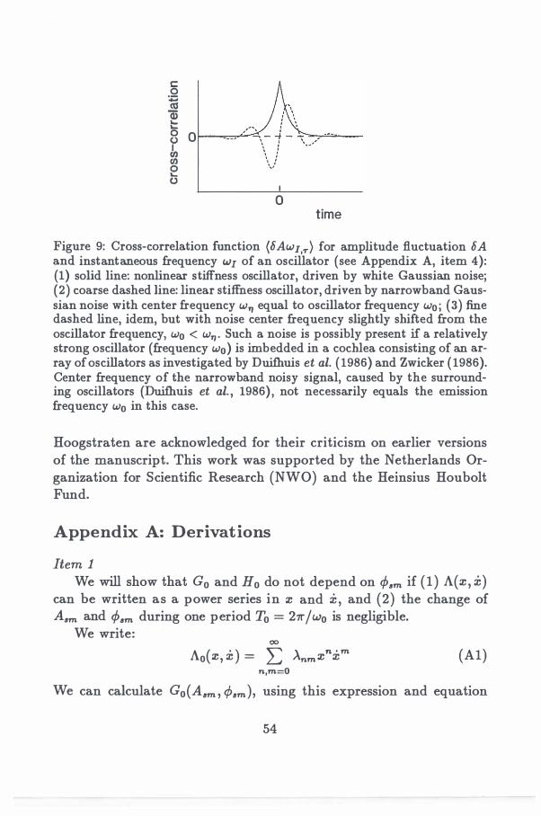
c: 0 � Q) 1: 8 0 r---=-==---·--·""-. Jn (/) e 0

0 time

Figure 9: Cross-correlation function (5Aw1,T) for amplitude fluctuation 5A and instantaneous frequency WI of an oscillator (see Appendix A, item 4): (1) solid line: nonlinear stiffness oscillator, driven by white Gaussian noise; (2) coarse dashed line: linear stiffness oscillator, driven by narrowband Gaussian noise with center frequency w11 equal to oscillator frequency wo; (3) fine dashed line, idem, but with noise center frequency slightly shifted from the oscillator frequency, w0 < ww Such a noise is possibly present if a relatively strong oscillator (frequency w0) is imbedded in a cochlea consisting of an array of oscillators as investigated by Duifhuis et al. ( 1986) and Zwicker (1986). Center frequency of the narrowband noisy signal, caused by the surrounding oscillators (Duifhuis et al. , 1986) , not necessarily equals the emission frequency w0 in this case.

Hoogstraten are acknowledged for their criticism on earlier versions of the manuscript. This work was supported by the Netherlands Organization for Scientific Research (NWO) and the Heinsius Houbolt Fund.

Appendix A: Derivations

Item 1 We will show that G0 and H0 do not depend on t/J.m if ( 1 ) A(:z:, :i:)

can be written as a power series in :z: and :i: , and (2) the change of Asm and t/J.m during one period T0 = 21rjw0 is negligible.

We write: 00

Ao(:z:, :i: ) = :2: Anm:z:":i:m (Al) n,m=O

We can calculate G0(Asm , tPsm), using this expression and equation

54

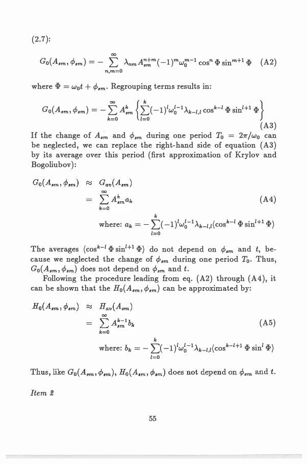
(2.7):

00

Go(Aam ' </>am) = - L AnmA�,!m( -l)mw;'-1 cosn � sinm+l � (A2) n,m=O

where � = w0t + <Pam · Regrouping terms results in:

Go(Aam ' <Pam) = - f: A=m {t( -1)1w�-1 Alc-l,l cosk-l � sin1+1 �} k=O l=O

(A3) If the change of Aam and </>am during one period T0 = 21r-jw0 can be neglected, we can replace the right-hand side of equation (A3) by its average over this period (first approximation of Krylov and Bogoliubov ):

(A4) k

where: a1c = - L(-1)1w�-1Aic-l ,l(coslc-l � sin1+1 �) l=O

The averages (coslc-l � sin1+1 �} do not depend on <Pam and t, because we neglected the change of <Pam during one period T0• Thus, Go(Aam , <Pam) does not depend on <f>,.m and t .

Following the procedure leading from eq. (A2) through (A4), it can be shown that the H0(Aam ' <Pam) can be approximated by:

(A5)

k where: b1c = - L( -1)1w�-1 Alc-l,z(cosk-l+l � sin1 �}

l=O

Item 2

55

We will show that if ( 1 ) A( x, x) can be written as a power series in x and :i: , and (2) the change of A6m and ¢.m during one period T0 = 2n-j w0 is negligible, then (a) the terms in A0 that contribute G au can be written as a function R( x, :i: ):i: , and (b) the terms in A0 that contribute Hau can be written as a function K(x, :i: )x, where R and K contain only term xn:i:m with n and m even:

The averages (cos4 <P sinb <P) in eq. (A4) and (AS) differ from zero, only if both a and b are even. Thus, in eq. (A3), only terms AJe-! ,zXk-lxl+l with k - l and l + 1 even, contribute to Gau Therefore, only terms AnmXn:i:m in A0 (eq. (A1)) , with n even and m odd, contribute to Gau · The sum of these terms can be written as R(x , :i: ):i:, where R contains only terms xn:i:m , with n and m even.

Using a similar argument , it can be concluded that only terms AnmXnxm in A0, with n odd and m even, contribute to Hau · The sum of these terms can be written as K ( x , :i: )x, where K contains only terms xnxm with n and m even.

Item 3 We will illustrate eq. (2 .44) and (2.45) for a special case: consider

a narrowband noise 71(t), with correlation function:

(A6)

with �w'1 � w'1 . The power spectral density S'l(w) of 7J equals the Fourier transforming of (7J7Jr) (Stratonovich, 1963a) :

S'l(w) = 2 1: eiwr (1J7Jr)dr 2�W'1 7J;m6 (A7)

since �w'1 � w'1 . Thus, most power of 71(t) is concentrated in a narrow band [w'l - �w'1, w'1 + �w'1] .

Using equations (2 .34) and (A6), we can calculate the correlation function for G1 ( t) :

2 (G1 Gl,r) = 1Jrr;• (e-Aw" lr l cos W'IT sin ¢o sin(woT + ¢o))

Wo

56

2 Tfrm11 e-�w, iri X 2w5 COS W11r(- cos(w0T + 2¢0) + COS WoT) (A8)

Since initial phase ¢0 is uniformly distributed, the first term between brackets averages to zero:

By Fourier transforming ( G1 G1,.,.) it can be shown that power spectral density Sa1 ( w) consists of two components located near respectively w = w0 - w11 and w = w0 + w11•

In Theory section we considered a narrowband noise with center frequency w11 equal to the oscillator frequency w0• Then:

(AlO)

The power spectral density of G1 follows from Fourier transforming equation (AlO) (Stratonovich, 1963a):

Sal ( w) = TJ�m�� { 4.6.w11 +

2.6.w11 } 4w5 w2 + .6.w� (w - 2w0)2 + .6.w�

� {s11(w + wo) + �S11(w - w0)} (All) 2w0 2

which is identical to equation (2.44) . A similar scheme can be followed to derive the spectral density of H1 (eq. (2.45)) .

Item 4 We will calculate the cross-correlation function (6Ahw1,.,.) for am

plitude fluctuation and instantaneous frequency fluctuation. First we will consider a linear stiffness oscillator (/3 = 0), driven

by narrowband noise TJ(t) , with correlation function given by (A6). If, .6.w11 � a: and w0 - w11 � a:, the low frequency component G1,Lp(t) of

57

G1 (t) (corresponding to the first term in eq. (A9)) falls entirely within the cutoff frequency a of amplitude equation (2.27), while the high frequency term (second term in eq. (A9)) is filtered out . Therefore, 8A(t) � a-1G1 ,£p(t). The cross-correlation function for amplitude and frequency can be written as (see equation (2.27) and (2.28):

(A12)

Cross-correlation between G1 and H1 can be calculated in a straight forward way:

2 71;rn

A, (e-Llw., J-rJ cos w'1(T ) sin ¢0 cos(woT + 4>o))

Wo o 2 11rrn, e -Llw11 J-rJ X

4w5Ao {sin( w'1 - w0 )T - sin( w'1 + w0 )T} (A13)

where we used that ¢0 is uniformly distributed. Substitution of this relation in eq. (A12), retaining only the low frequency term, yields:

2 (h'A w ) = 1Jrrn, e-Llw., J-rl sin(w - w )T I,-r 4 2A '7 o

Wo o (A14)

Fig.9 displays (8A wi,-r) for w'1-w0 > 0 (fine dashed line) and w0 -w'1 =

0 (coarse dashed line) . In the latter case (8Aw1,.,.) = 0, i.e. amplitude and frequency are statistically independent .

As second example, we calculate (8Aw1,.,.) for a nonlinear stiffness oscillator. We will assume that the first term in the right-hand side of equation (2.28) , dominates over the second. Consequently, 8w1(t) =

8¢(t) � f38A(t) , and the cross-correlation function between amplitude and frequency is proportional to the amplitude correlation function:

(A15)

As example, we consider a white Gaussian noise excitation of the oscillator. Then (8A8A.,.) = S.,., x (8aw5)-1 exp( -a iT I ) (inverse Fourier transform of Su(w) in eq. (2.38)). Substitution in eq. (A15) yields:

(A16)

See Fig. 9, solid line.

58

Appendix B : Zerocrossings of a sinusoid plus narrowband noise

We will consider zerocrossings of the signal:

:z: = A sin(w0t + ¢) + � (B1)

We will assume the amplitude A and phase ¢ to exhibit small fluctuations, similar to the amplitude and phase fluctuation of spontaneous otoacoustic emissions. The function e(t) is a noise function, which corresponds to the microphone noise in the emission recordings. As described in the Material and Methods section, we determined zerocrossings of bandpass filtered microphone signals. The center frequency of the bandpass filter was chosen to be equal to the emission frequency. Consequently, we let e be a narrowband noise process , with center frequency at w0•

Consider :z: as function of ii = (A, ¢, e ' t ) . Then, for R

o =

(A0 , O, O, 21rnjw0) (where n = 0, 1 , 2, · · · counts successive zerocrossings) , we have z(Ro) = 0. Expanding :z:(R0 + AR) in a Taylor series yields:

z(ii. + t>ii) z(ii.) +t>A :�Iii, + M =:Iii, ue �;Iii, +

At 8:z: l + · · · 8t Ro � A� + A0 (w0At + A¢) (B2)

Zero crossings of :z:( R0 + AR) occur at times given by:

(B3)

which gives the time between two successive zero crossing (with n = i and n = i - 1) :

(B4)

Thus, the time between successive zerocrossing only depends on A� and A¢ . Since both are uncorrelated to each other, the spectrum of

59

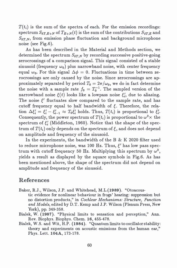
T(ti) is the sum of the spectra of each. For the emission recordings: spectrum s6T,E+N of TE+N(t) is the sum of the contributions s6T,E and S6T,N1 from emission phase fluctuation and background microphone noise (see Fig.6).

As has been described in the Material and Methods section, we determined the spectrum S6T,N by recording successive positive-going zerocrossings of a comparison signal. This signal consisted of a stable sinusoid (frequency w0) plus narrowband noise, with center frequency equal w0• For this signal A</> = 0 . Fluctuations in time between zerocrossings are only caused by the noise. Since zerocrossings are approximately separated by period T0 = 27r /w0, we do in fact determine the noise with a sample rate /0 = T0-1 • The sampled version of the narrowband noise e(t) looks like a lowpass noise e:, due to aliasing. The noise e' fluctuates slow compared to the sample rate, and has cutoff frequency equal to half bandwidth of e. Therefore, the relation A.ei = e: - eL1 � Toei holds. Thus, T( ti) is proportional to e:. Consequently, the power spectrum of T( ti ) is proportional to w2 x the spectrum of e: (Middleton, 1960). Notice that the shape of the spectrum of T( ti ) only depends on the spectrum of e , and does not depend on amplitude and frequency of the sinusoid.

In the experiments, the bandwidth of the B & K 2020 filter used to reduce microphone noise, was 100 Hz. Thus, e' has low pass spectrum with cutoff frequency 50 Hz. Multiplying this spectrum by w2 , yields a result as displayed by the square symbols in Fig.6. As has been mentioned above, the shape of the spectrum did not depend on amplitude and frequency of the sinusoid.

References

Baker, R.J., Wilson, J .P. and Whitehead, M.L.(1989) . "Otoacous-tic evidence for nonlinear behaviour in frogs ' hearing: suppression but no distortion products," in Cochlear Mechanisms: Structure, Function and Models, edited by D.T. Kemp and J.P. Wilson (Plenum Press, New York), pp. 349-358.

Bialek, W. (1987). "Physical limits to sensation and perception," Ann. Rev. Biophys. Biophys. Chern. 16, 455-478.

Bialek, W.S. and Wit , H.P. (1984). "Quantum limits tooscillator stability: theory and experiments on acoustic emissions from the human ear,"

Phys. Lett. 104A, 173-178.

60

Dallmayr, C . (1985) . "Spontane otoakustische Emissionen, Statistik and Reaktion auf akustische Stortone," Acustica 59, 67-75.

Dallas, P. (1988). "Cochlear neurobiology: some key experiments and concepts of the past two decades," in Auditory Function: Neurobiological Bases of Hearing, edited by W.E. Call and W.M. Cowan (Wiley, New York) , pp. 153-188.

Duffing, G. (1918). Erzwungene Schwingungen bei Veriinderliche Eigenfrequenz (Vieweg und Sohn, Braunsweig) .

Duifhuis, H. , Hoogstraten, H.W., van Netten, S .M., Diependaal, R.J., and Bialek, W. (1986) . "Modelling the cochlear partition with coupled Van der Pol oscillators," in Peripheral Auditory Mechanisms, edited by J.B . Allen, J.L. Hall, A. Hubbard, S .T. Neely, and A. Tubis (Springer, Berlin), pp. 290-297.

Fritze, W. (1983) . "Registration of spontaneous cochlear emissions by means of Fourier transformation," Arch. Otorhinolaryngol. 238, 189-196.

Furst, M. (1989} . "Reply to "Comment on 'A cochlear model for acoustic emissions ' " [J . Acoust . Soc. Am . 85, 2217 (1989 ) ] ," J. Acoust . Soc. Am. 85, 2218-2220.

Furst, M., and Lapid, M. (1988) . "A cochlear model for acoustic emissions," J . Acoust . Soc. Am. 84, 222-229.

Gold, T. (1948) . "Hearing II. The physical basis of the action of the cochlea," Proc. R. Soc. Ed. B135, 492-498.

Guckenheimer, J . , and Holmes, P. (1983). Nonlinear Oscillations, Dynamical Systems, and Bifurcations of Vector Fields (Springer, New York) , Chap. 1 and 2, pp. 1-116.

Haggerty, H. (1989). personal communication. Hanggi, P. , and Riseborough, P. (1982). "Dynamics of nonlinear dissipa

tive oscillators," Am. J. Phys. 51, 347-352. Harris, F.J. (1978). "On the use of windows for harmonic analysis with

discrete Fourier transform," Proc. IEEE 66, 51-83. Hsu, H.P. 1967). Fourier Analysis (Simon and Schuster, New York) , pp.

11-13. Johannesma, P.I.M. (1980). "Narrowband filters and active resonators,"

in Psychophysical, Physiological and Behavioural Studies in Hearing, edited by G. van den Brink and F.A. Bilsen (Delft University Press, Delft) , pp 62-63.

Kemp, D.T. (1979) . "Evidence for mechanical nonlinearity and frequency selective wave amplification in the cochlea," Arch. Otorhinolaryngol. 224, 37-45.

Koshigoe, S . , and Tubis, A. (1983) . "A non-linear feedback model for outer-hair-cell stereocilia and its implications for the response of the auditory periphery," in Mechanics of Hearing, edited by E. de Boer and M.A. Viergever (Nijhoff, The Hague), pp. 127-134.

61

Kohler, W., Fredriksen, E. , and Fritze, W. (1986) . "Spontaneous otoacoustic emissions - a comparison of the left versus the right ear," Arch. Otorhinolaryngol. 243, 43-46.

Lewis, E.R. , Leverenz, E.L., and Bialek, W.S. (1985). The Vertebrate Inner Ear ( CRC Press, Boca Raton), p . 222.

Long, G.R. and Tubis A. (1988) . "Modification of spontaneous and evoked otoacoustic emissions and associated psychoacoustic microstructure by aspirin consumption," J. Acoust . Soc. Am. 84, 1343-1353.

Long, R.L. , Tubis, A., Jones, K.L. , and Sivaramakrishnan, S. (1989) . "Modification of the external-tone synchronization and statistical properties of spontaneous otoacoustic emissions by aspirin consumption," in Basic Issues in Hearing, edited by H.Duiihuis, J .W. Horst, and H.P. Wit (Academic Press, London), pp. 93-100.

Middleton, D. (1960) . An Introduction to Statistical Communication Theory (McGraw Hill Book Company, New York) , pp. 606-610.

Millman, J. , and Halkias, C .C . (1972) . Integrated Electronics: Analog and Digital Circuits and Systems (Me Graw-Hill, New York), pp. 1 14-115.

Nayfeh, A.H., and Mook, D.T. (1979) . Nonlinear Oscillation (Wiley and Sons, New York) , pp. 62-63.

Palmer, A.R., and Wilson, J .P. (1981 ) . "Spontaneous and evoked acoustic emissions in the frog Rana esculenta," J. Physiol. (Lond. ) 324, 64P.

Papoulis, A. (1984). Probability, Random Variables, and Stochastic Processes (McGraw-Hill, Auckland) , pp. 314-330.

Rebillard, G. , Abbou, S., and Lenoir, M. {1987). "Les oto-emission acoustic II. Les oto-emission spontanees: resultats chez des sujets normaux ou presentant des acouphEmes," Ann. Oto-Laryng. (Paris) 104, 363-368.

Ruggero, M.A., Rich, N.C. , and Freyman, R. (1983) . "Spontaneous and impulsively evoked otoacoustic emissions: indicators of cochlear pathology?," Hear. Res. 10, 283-300.

Schloth, E. ( 1983 ) . "Relation between spectral composition of spontaneous oto-acoustic emissions and :fine-structure of threshold in quiet ," Acustica 53, 250-256.

Schloth, E. and Zwicker, E. (1983) . "Mechanical and acoustical influences of spontaneous oto-acoustic emissions," Hear. Res. 11 , 285-293.

Stoker, J.J. (1950) . Nonlinear Vibrations (Wiley and Sons, New York) , Chap. 6, pp . 81-118.

Stratonovich, R.L. (1963a). Topics in the Theory of Random Noise, Volume I (Gordon and Breach, New York) , Chap. 1 , and 2, pp. 3-37.

Stratonovich, R.L. (1963b) . Topics in the Theory of Random Noise, Volume !/ (Gordon and Breach, New York) , Chap. 4, 5, and 6, pp. 87-169.

Strickland, E.A. , Burns, E.M. , and Tubis, A. (1985) . "Incidence of spontaneous otoacoustic emissions in children and infants," J . Acoust . Soc. Am. 78, 931-935.

Tubis, A., Long, G.R. , Sivaramakrishan, S. and Jones, J.L. (1989).

62

"Tracking and interpretive models of the active-nonlinear cochlear response during reversible changes induces by aspirin consumption," in Cochlear Mechanisms: Structure, Function and Models, edited by D.T. Kemp and J.P. Wilson (Plenum Press, New York) , pp. 323-330.

van der Pol, B. ( 1927) . "Forced oscillation in a circuit with nonlinear resistance (receptance with reactive triode) ," London, Edinburg and Dublin Phil. Mag. 3, 65-80.

van Dijk, P., and Wit, H.P. (1988) . "Phase-lock of spontaneous otoacoustic emissions to a cubic difference tone," in Basic Issues in Hearing, edited by H. Duifhuis, J.W. Horst and H.P. Wit (Academic Press, London) , pp. 101-105.

van Dijk, P., Wit , H.P. and Segenhout, J.M. (1989). "Spontaneous otoacoustic emissions in the European edible frog (Rana esculenta): Spectral details and temperature dependence," Chapter 3 of this thesis and Hear. Res. 42, 273-282.

van Netten, S.M., and Duifhuis, H. ( 1983) . "Modelling and active, nonlinear cochlea," in Mechanics of Hearing, edited by E. de Boer and M.A. Viergever (Nijhoff, The Hague) , pp. 143-151.

Wilson, J .P. (1980) . "Evidence for a cochlear origin for acoustic reemissions, threshold fine-structure and tonal tinnitus," Hear. Res. 2, 233-252.

Wilson, J.P., Whitehead, M.L., and Baker, R.J. (1986). "The effect of temperature in otoacoustic emission tuning properties," in Auditory Frequency Selectivity, edited by B.C.J. Moore and R.D. Patterson (Plenum Press, London) , pp. 39-46.

Wit, H.P. (1985) . "Diurnal cycle for spontaneous oto-acoustic emission frequency," Hear. Res. 85, 197-199.

Wit, H.P. (1986). "Statistical properties of a strong otoacoustic emission," in Peripheral Auditory Mechanisms, edited by J.B. Allen, J.L. Hall, A. Hubbart, S.T. Neely, and A. Tubis (Springer Press, Berlin) , pp. 137-146.

Wit , H.P., Langevoort , J.C. and Ritsma, R.J. (1981) . "Frequency spectra of cochlear acoustic emissions ( 'Kemp-echoes') ," J. Acoust. Soc. Am .

70, 437-445. Ziss, C.A., and Glattke, T.J. (1988) . "Reliability of spontaneous otoacous

tic emission suppression tuning curve measurement," J. Sp. Hear. Res. 31 , 616-619.

Zurek, P.M. (1981) . "Spontaneous narrowband acoustic signals emitted by human ears," J . Acoust. Soc. Am. 69, 514-523.

Zwicker, E. (1986) . " 'Otoacoustic' emissions in a nonlinear cochlea hardware model with feedback," J. Acoust. Soc. Am. 80, 154-162.

63

Chapter 3

SPONTANEOUS OTOACOUSTIC EMISSIONS IN THE EUROPEAN EDIBLE FROG (RANA ESCULENTA ) ; SPECTR A L DETAILS AND TEMPER ATURE DEPENDENCE.

Abstract

Spontaneous otoacoustic emissions were recorded in 41 ears of 29 European edible frogs (R. esculenta). Emission frequencies ranged from 450 to 1350 Hz. The distribution of frequencies shows two distinct populations: one above and one below 1 kHz. With one exception, a maximum number if two emissions was recorded per ear, each in a different population. An amplitude distribution of a frog emission was sampled, from which it was concluded that the emission is generated by an active oscillator. The spectral width of an emission ranged from 1 to 200 Hz (average 38 Hz). There was negative correlation between sound pressure level of an emission and spectral width. In 4 frogs the dependence of emission power and frequency on temperature was investigated. An emission could be "switched on and off'' within a few degrees centigrade. At temperatures below the switching interval no emission was recorded; for higher temperatures emission power showed no dependence on temperature. Frequency increased with temperature ( Q10 =1 .1 to 1 .3) . This yields a mismatch with temperature dependence of best frequencies of auditory fibers. The consequences of this mismatch are discussed.

65

Introduction

In 1978 Kemp reported emission of acoustical energy from the human ear in response to a click stimulus in the ear canal. Later experiments also showed that narrow band acoustical signals can be emitted by the ear without a stimulus (Kemp, 1979; Zurek, 1981) . These spontaneous otoacoustic emissions are considered to represent a strong argument in favour of active signal processing in the inner ear. As long ago as 1948, had Gold argued that active signal processing in the ear is necessary in order to overcome interference of internal noise in the ear. He predicted emission of acoustical energy by the ear, as a byproduct of the active process. Several experiments show that otoacoustic emissions are indeed generated by the inner ear: 1 . frequency of spontaneous otoacoustic emissions closely corresponds to SPL-minima in the pure-tone threshold curve (Schloth, 1983; Horst et al. 1983; Long and Tubis, 1988). 2. suppression of otoacoustic emissions by a pure-tone stimulus yields iso-suppression tuning curves (Kemp, 1979; Wilson, 1980; Wit et al. , 1981 ; Schloth and Zwicker, 1983; Ziss and Glattke, 1988), with a shape similar to neural tuning curves in other mammals (Kiang and Moxon, 1974). Besides the cochlear origin of otoacoustic emissions, these experiments provide evidence for a relation between otoacoustic emissions and tuning mechanisms responsible for the frequency selectivity of the cochlea.

Palmer and Wilson ( 1981 ) measured evoked and spontaneous otoacoustic emissions in frogs. Baker et al. (1989) measured isosuppression tuning curves of spontaneous emissions in frogs. They were similar to neural tuning curves (Narins and Hillery, 1983). Thus, as with humans, the generation mechanism for otoacoustic emissions in frogs is probably related to the frequency selectivity of the frog ear.

The existence of otoacoustic emissions in frogs is intriguing since they have simple hearing organs, as compared to the mammalian ear. The inner ear contains two hearing organs, the amphibian and the basilar papilla. There is no structure similar to the organ of Corti. In both organs, the hair cells are imbedded in a relatively solid structure. No basilar membrane exists. Haircells are not morphologically distinct , like inner and outer hair cells in the mammalian cochlea (for a review see Lewis et al., 1985) .

66

We will report various features of frog spontaneous emissions such as their amplitude distribution and the relation between spectral width and sound pressure level (SPL) of an emission. The consequences for a model of the frog emissions are discussed. Also, we will present the distribution of emission frequencies and discuss it in relation to the frequency sensitivity ranges and anatomy of both papillae in the frog ear.

Because frogs are ectothermic animals, their body temperature can be varied over a large temperature interval. The frequency of simultaneous evoked frog otoacoustic emissions shows a significant dependence on body temperature (Wilson, 1986). In this work, we investigated both power and frequency of spontaneous otoacoustic emissions in frogs as function of temperature. Results are compared to temperature dependence of neural response in the auditory nerve. The comparison provides a test for the hypothesis that emission generation mechanisms are related to frequency selectivity in the inner ear. The relation between emissions and electrical haircell oscillations is also discussed.


Spontaneous otoacoustic emission measurements were performed in 29 European edible frogs (Rana esculenta) . Frogs were anesthetized via immersion in a 0.1% MS 222 solution, prior to the experiment . During the experiment the frog was covered by a thin gauze, drained in the MS 222 solution. In an earlier stage of the present experiments, frogs were anesthetized by injection of 1 cc 0.6% pentobarbital solution per 100 g body weight . Emissions could also be measured in non-anesthetized frogs. This was done at low temperatures (10 to 15°C), in which frogs are very inactive.

Emissions were measured with a sensitive condenser microphone (Wit et al. , 1981 ) . This microphone is most sensitive between 1 and 2 kHz; with an analyzing bandwidth of 4 Hz a sinusoidal signal of 0 dB SPL is more than 20 dB above the noise of the measuring system. During an experiment, the microphone signal was recorded on video tape after pulse code modulation (SONY digital audio processor PCM-F1) .

67

Emissions could be measured either by connecting the microphone with a small tube to the tympanic membrane of the frog, or by gently fitting a small tube through the mouth into the Eustachian tube of the frog. When using the first method, emissions from both ears could be recorded by the microphone, due to good acoustic coupling between both middle ears of the frogs (Vlaming et al. , 1981) . With the latter method, acoustic coupling between the two middle ears was obstructed. Thus, only emissions from one ear were detected by the microphone.

Recorded microphone signals were Fast Fourier transformed, using a Unigon 4512 spectrum analyzer. Peaks in the spectrum, corresponding to spontaneous otoacoustic emissions, were fitted with a Lorenzian curve. Sound pressure level, frequency and spectral width of an emission could be determined from the resulting fit parameters . For further characterization of the emission signals, an amplitude distribution was determined, using a DATALAB DT4000 system. This was done after bandpass filtering the microphone signal, in order to reduce the noise from the measuring system (filter:B&K 2020, �f_3dB = 100Hz).

The influence of body temperature on emissions was investigated in 4 frogs. To regulate the frog's temperature, the animal was placed in a water bath. The water was cooled or heated by Peltier devices underneath the bath. The frog's temperature was measured with a small thermocouple in the mouth. Typical cooling and heating rates between measurements were 0.5°C/minute. The microphone signal was recorded at various temperatures. The microphone signal was monitored on line with the spectrum analyzer. In order to pick up emissions from both ears, the microphone was connected to the tympanic membrane, during the temperature experiments . Off line, recorded signals were Fast Fourier transformed and further analyzed as described above.

Results

Fig. la shows spectra of the microphone signal as recorded in two frog ears. Spontaneous otoacoustic emissions are visible as peaks in the spectrum. Fig. 1 b displays the spectrum of the 1 182 Hz emission of frog 2 in Fig. la with expanded frequency axis. The solid curve

68

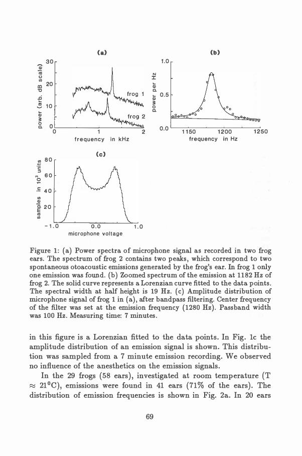
(a) (b) 30 1 .0 ......

Ql (ij N 0 J: rn

20 .... m Ql "C c.

..ci .... 0.5 Ql .... ;: al 1 0 0

.... c. Ql 0 ;: 0 0 c. 0.0 0 2 1 1 50 1 200 1 250

frequency in kHz frequency in Hz

(c) rn 8 0

-·c: :J

M 6 0 0 ,.... ·= 4 0 rn Q)

a. 2 0 E al rn

- 1 . 0 1 . 0 microphone voltage

Figure 1 : (a) Power spectra of microphone signal as recorded in two frog ears. The spectrum of frog 2 contains two peaks , which correspond to two spontaneous otoacoustic emissions generated by the frog's ear. In frog 1 only one emission was found. (b) Zoomed spectrum of the emission at 1182 Hz of frog 2. The solid curve represents a Lorenzian curve fitted to the data points. The spectral width at half height is 19 Hz. (c) Amplitude distribution of microphone signal of frog 1 in (a) , after bandpass filtering. Center frequency of the filter was set at the emission frequency (1280 Hz) . Passband width was 100 Hz. Measuring time: 7 minutes.

in this figure is a Lorenzian fitted to the data points. In Fig. lc the amplitude distribution of an emission signal is shown. This distribution was sampled from a 7 minute emission recording. We observed no influence of the anesthetics on the emission signals.

In the 29 frogs (58 ears) , investigated at room temperature (T � 21 °C), emissions were found in 41 ears (71% of the ears) . The distribution of emission frequencies is shown in Fig. 2a. In 20 ears

69

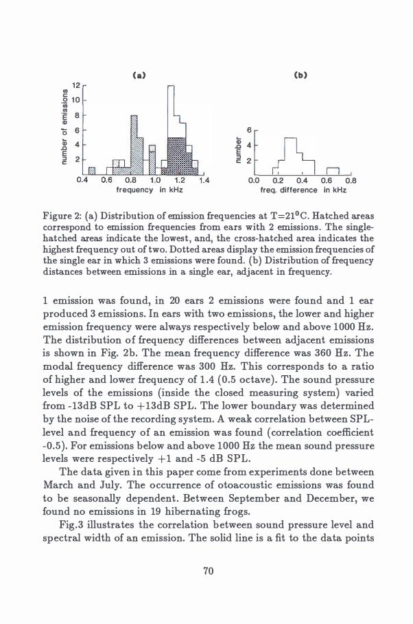
(a) (b) 12

Ill c: .2 10 Ill Ill

·e 8 Q)

- 6

: r 0 ... ...

A Q) 4 Q)

.0 .0 E E :::1 2 :::1 c: c:

n I 0.0 0.2 0.4 0.6 0.8 frequency in kHz freq. difference in kHz

Figure 2: (a) Distribution of emission frequencies at T=21 °C. Hatched areas correspond to emission frequencies from ears with 2 emissions. The singlehatched areas indicate the lowest, and, the cross-hatched area indicates the highest frequency out of two. Dotted areas display the emission frequencies of the single ear in which 3 emissions were found. (b) Distribution of frequency distances between emissions in a single ear, adjacent in frequency.

1 emission was found, in 20 ears 2 emissions were found and 1 ear produced 3 emissions. In ears with two emissions, the lower and higher emission frequency were always respectively below and above 1000 Hz. The distribution of frequency differences between adjacent emissions is shown in Fig. 2b. The mean frequency difference was 360 Hz. The modal frequency difference was 300 Hz. This corresponds to a ratio of higher and lower frequency of 1 .4 (0.5 octave) . The sound pressure levels of the emissions (inside the closed measuring system) varied from -13dB SPL to +13dB SPL. The lower boundary was determined by the noise of the recording system. A weak correlation between SPLlevel and frequency of an emission was found (correlation coefficient -0.5). For emissions below and above 1000 Hz the mean sound pressure levels were respectively + 1 and -5 dB SPL.

The data given in this paper come from experiments done between March and July. The occurrence of otoacoustic emissions was found to be seasonally dependent . Between September and December, we found no emissions in 19 hibernating frogs.

Fig.3 illustrates the correlation between sound pressure level and spectral width of an emission. The solid line is a fit to the data points

70

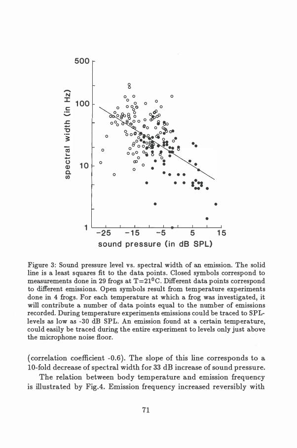
500

-N J: 1 00 c: -� -"C � ca � -0 1 0 Q) a. rn

1

8 0 0 0 0 0

0 0 0� 0 0 oogb� g oOlcP 0 O O O �i eo 0 0 0 0 0 0 �

0

0 0

0

-25

0 0 cit o oO o � • 0 • 0 • eo ••o II o o o o .. e o oO oi ! � 0 0 • (S) • • • 0 0 • • • • • • • •

•

- 1 5 -5

••

.... .. .

• 5

sound pressure ( in dB SPL)

•

1 5

Figure 3: Sound pressure level vs. spectral width of an emission. The solid line is a least squares fit to the data points. Closed symbols correspond to measurements done in 29 frogs at T=21 °C. Different data points correspond to different emissions. Open symbols result from temperature experiments done in 4 frogs. For each temperature at which a frog was investigated, it will contribute a number of data points equal to the number of emissions recorded. During temperature experiments emissions could be traced to SPLlevels as low as -30 dB SPL. An emission found at a certain temperature, could easily be traced during the entire experiment to levels only just above the microphone noise floor.

(correlation coefficient -0.6) . The slope of this line corresponds to a 10-fold decrease of spectral width for 33 dB increase of sound pressure.

The relation between body temperature and emission frequency is illustrated by Fig.4. Emission frequency increased reversibly with

71

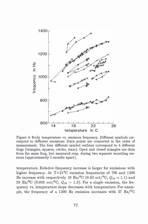
1 400

1 200

N J: c::

>. 1 000 (.) c:: Q) ::J 0' Q) a...

-

800

600 1 4 1 8 2 2 26 temperature in C

Figure 4: Body temperature vs. emission frequency. Different symbols correspond to different emissions. Data points are connected in the order of measurement . The four different symbol outlines correspond to 4 different frogs (triangles, squares, circles, stars ) . Open and closed triangles are data from the same frog, but measured resp. during two separate recording sessions (approximately 2 months apart ) .

temperature. Relative frequency increase is larger for emissions with higher frequency. At T=21 °C emission frequencies of 700 and 1200 Hz increase with respectively 10 Hz/°C (0 .02 oct/°C, Q10 = 1 .1 ) and 29 Hz/°C (0.035 oct/°C, Q10 = 1 .3). For a single emission, the frequency vs. temperature slope decreases with temperature. For example, the frequency of a 1200 Hz emission increases with 37 Hz/°C

72

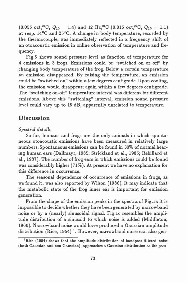
(0.055 oct/00, Q10 = 1 .4) and 12 Hz/00 (0.015 oct/00, Q10 = 1 .1) at resp. 14°0 and 25°0. A change in body temperature, recorded by the thermocouple, was immediately reflected in a frequency shift of an otoacoustic emission in online observation of temperature and frequency.

Fig.5 shows sound pressure level as function of temperature for 4 emissions in 3 frogs. Emissions could be "switched on or off'' by changing body temperature of the frog. Below a certain temperature an emission disappeared. By raising the temperature, an emission could be "switched on" within a few degrees centigrade. Upon cooling, the emission would disappear; again within a few degrees centigrade. The "switching on-off'' temperature interval was different for different emissions. Above this "switching" interval, emission sound pressure level could vary up to 15 dB, apparently unrelated to temperature.

Discussion

Spectral details So far, humans and frogs are the only animals in which sponta

neous otoacoustic emissions have been measured in relatively large numbers. Spontaneous emissions can be found in 30% of normal hearing human ears (Dallmayr, 1985; Strickland et al. , 1985; Rebillard et al. , 1987). The number of frog ears in which emissions could be found was considerably higher (71%). At present we have no explanation for this difference in occurrence.

The seasonal dependence of occurrence of emissions in frogs, as we found it , was also reported by Wilson (1986). It may indicate that the metabolic state of the frog inner ear is important for emission generation.

From the shape of the emission peaks in the spectra of Fig.1a it is impossible to decide whether they have been generated by narrowband noise or by a (nearly) sinusoidal signal. Fig.1c resembles the amplitude distribution of a sinusoid to which noise is added (Middleton, 1960). Narrowband noise would have produced a Gaussian amplitude distribution (Rice, 1954) 1 . However, narrowband noise can also gen-

1Rice (1954) shows that the amplitude distribution of bandpass filtered noise (both Gaussian and non-Gaussian) , approaches a Gaussian distribution as the pass-

73

...J a. en m "0 c:

Q) .... � en en Q) .... a.

"0 c: � 0 en

0

�rr - 1 0

-20

0

- 1 0 i(; -20

-3��5��--�2�0�--�l-��2 5 temperature in C

Figure 5 : Body temperature vs. emission sonnd pressure level. Symbols correspond to those in Fig. 4. Arrows indicate the order in which the data points were measured. The experiment illustrated in the upper panel started at T=19.5°C . Two emissions were recorded at this temperature, of which one is displayed. While warming up the frog, another emission appeared at T=22.5°C. This emission raised to its final level of approximately -10 dB SPL within a few degrees centigrade. Cooling down the frog, resulted in disappearance of this emission at T=21 .5°C. The other emission remains constant within 8 dB during the entire experiment . "Switching on and off'' of an emission is also demonstrated in the lower panel. These data correspond to emissions in different frogs. The stars display results of an experiment in which an emission was switched on and off several times. This experiment started at approximately T=23°C. At that temperature the emission level was -15 dB SPL. The frog was warmed up to T=25°C and subsequently cooled to T=20°C . Cooling caused the emission to disappear at T=22.5°C . When heating the frog again, up to T=24.5°C, the emission reappeared at T=21 °C . Again cooling the frog from T=24.5°C to 20°C caused the emission to disappear at T=23°C . Finally, warming up caused the emission to reappear at T=22°C.

74

erate an amplitude distribution like Fig. 1c if the measuring time is smaller than the correlation time of the noise. The spectral width of a frog emission is in the order of 10 Hz. If the peak were generated by narrowband noise, the corresponding correlation time would be 10-1

s. For Fig. 1c the measuring time was 7 minutes, which is three orders of magnitude longer than this correlation time. Thus, it is safe to conclude that Fig. 1c is generated by a sinusoidal signal and consequently, that the peaks in the spectra of Fig. 1a are generated by sinusoidal signals. A similar amplitude distribution can be found for human emissions (Bialek and Wit , 1984; Wit , 1986) . Therefore, as human emissions, frog emissions are generated by an active oscillatory process.

With one exception, a maximum number of two emission could be found in each frog ear. Human ears can produce more then 10 spontaneous emissions per ear (Dallmayr, 1985) , with an average of approximately 3 per emitting ear (Dallmayr, 1985; Strickland et al. , 1985) If haircells are responsible for the generation of otoacoustic emissions, this could reflect the difference in number of haircells present in respectively the frog and the human ear. The amphibian and basilar papillae of frogs contain roughly 1500 and 100 haircells (Lewis et al. , 1985) . The human cochlea contains about 16,800 haircells (Bredberg, 1986) .

The frequency distribution of Fig. 2a shows two distinct populations of emissions, one above and one below 1 kHz. Both shaded areas in Fig. 2a are either strictly above or below 1 kHz. Thus, the two emissions were always in a different population. For the American bullfrog, Lewis et al. (1982) showed that the amphibian papilla is sensitive to frequencies below 1 kHz and the basilar papilla to frequencies above 1 kHz. If, for Rana esculenta the amphibian and basilar papillae are sensitive to the same frequency ranges, then each population in Fig. 2a represents emissions generated in one of the two papillae. On the other hand, the frequency range of each papilla is known to be species dependent . In some anuran species the amphibian papilla is sensitive up to 1 .4 kHz (for a review see Zakon and Wilczynski, 1988) . The fact that Wilson (1986) only reports emissions below 1 kHz in R. temporaria also indicates species differences. Like in the R. tern-

band is narrowed.

75

poraria, we barely found emissions below 600 Hz. However, we could have missed emissions due to reduced sensitivity of the microphone in that frequency range.

In the above discussion, we assume that an emission is generated at the location in the inner ear most sensitive to sound with frequencies close to the emission frequency. In humans this is made very likely by the shape of suppression tuning curves of oto-acoustic emissions (Kemp, 1979; Wilson, 1980; Wit et al. , 1981; Schloth and Zwicker, 1983; Ziss and Glattke, 1988) . Suppression is maximal for suppressing tones with frequencies close to the emission frequency and the shape is similar to neural tuning curves found in other mammals (for example see Kiang and Moxon, 1974). Tubis et al. (1989) showed that suppression of an emission can be modeled by a Van der Pol oscillator located at the spot on the basilar membrane most sensitive to sound with frequency of the oscillator. This shows that an emission generator located at such a position can exhibit the suppression behaviour found in experiments. Also, the relation between emission frequencies and maxima and minima in microstructure of the pure tone audiogram (Schloth, 1983; Horst et al. , 1983; Long and Tubis, 1988) , indicates that emissions are generated at a location on the basilar membrane most sensitive to sound with emission frequency. Baker et al. (1989) measured suppression tuning curves in frogs. The asymmetry of these suppression curves, similar to neural tuning curves (Narins and Hillery, 1983) , again suggests generation of the emission near the place of optimum sensitivity of the hearing organ. Thus, a considerable amount of experimental evidence supports emission generation at a location in the inner ear most sensitive to sound with emission frequency. However, the results of the temperature experiments discussed at the end of this section, bring this assumption into question.

The modal frequency distance of 0.5 octave between 2 emissions in one frog ear is significantly larger than the value of 0.1 octave found in humans (Dallmayr, 1985, 1987; Zwicker and Schloth, 1984). As Zwicker (1988) shows, locations on the human basilar membrane sensitive to frequencies 0.1 octave apart, are excited with a phase difference of 180° by a traveling cochlear wave. Therefore, the 0.1 octave distance in humans could reflect the involvement of standing waves

76

on the basilar membrane, in the generation of otoacoustic emissions. No basilar membrane exists in frogs. The haircells are imbedded in a relatively stiff structure. The different frequency distance of 0.5 octave is thus not surprising. Two important cochlear features in Zwickers discussion of the 0.1 octave frequency distance, are also present in the amphibian papilla: there is evidence for a traveling wave in the tectorial membrane (Hillery and Narins, 1984; Lewis, 1984) and the amphibian papilla is tonotopically organized (Lewis et al. , 1982). If we assume that (1 ) all frog emissions are generated in the amphibian papilla, and (2) standing waves are involved in the generation of the emissions, then the 0.5 octave frequency distance between two frog emissions reflects the mechanical properties of the tectorial membrane.

The spectral width of a frog emission can vary between 1 and 200 Hz. All data points in Fig. 3 yield an average width of 38 Hz. In humans the spectral width of a spontaneous otoacoustic emission is typically 1 Hz (van Dijk and Wit , 1988; Wit and van Dijk, 1989). Thus, the frequency fluctuations of frog emissions are one order of magnitude larger than for human emissions. The data points in Fig. 3 corresponding to temperature experiments (open symbols) , determined in 4 frogs at different temperatures, follow the same trend as those found in 29 frogs at room temperature (closed symbols) . Thus, the spectral width of an emission is related to power of the emission, rather than to temperature. The relation between temperature and spectral width, has its origin in the relation between temperature and power. It has been shown that an emission can be modelled by a Van der Pol oscillator (Johannesma, 1980; Long and Tubis, 1988; Tubis et al. , 1989) driven by a randomly fluctuating noise force (Bialek and Wit, 1984; van Dijk and Wit, 1988). With a suitable choice of oscillator parameters and in the absence of noise, the Van der Pol oscillator will exhibit a sinusoidal oscillation. Consequently, the spectral width of this oscillation is 0 Hz. Noise causes the spectrum to broaden over a certain spectral width. It can be shown (Stratonovich, 1963) that this width is given by:

�W = S6F(w) 8A2K-m (1 )

where, (for a mechanical oscillator) K. and m are stiffness and mass,

77

determining the oscillator frequency w = J K / m, A is the oscillation amplitude and S5F( w ) is the power spectral density of the noise force SF acting on the oscillator. If the noise level is kept constant, and the amplitude of the emission is increased, the spectral width of the oscillation becomes smaller. A similar trend is observed in Fig. 3 . As follows from the above equation, a 10 dB increase in oscillation power (proportional to A2) would result in an 10-fold decrease of spectral width. Fig. 3 however, shows that a 33 dB increase of power is necessary for a 10-fold decrease of spectral width. One possible explanation could be that the noise causing the broadening of the spectrum is not a constant , but a function of the amplitude, i.e. of the total power emitted. The noise would then be inherent to the process responsible for generation of emissions, rather than being one "external" noise source to which all emission generators are submitted. On the other hand, this result could indicate that a Van der Pol oscillator does not provide completely adequate means of describing otoacoustic emissions.

Temperature effects The frequency of a spontaneous otoacoustic emission shows a clear

and reversible dependence on temperature. Wilson et al. (1986) found a similar change with temperature for simultaneous evoked emissions in R. temporaria. Thus, as in humans (Wit et al. , 1981; Probst et al., 1986; Zwicker, 1988) , spontaneous and evoked emissions in frogs probably have a common source. Changes of emission frequency with temperature in humans were investigated by Wilson (1985) . His experiments were not conclusive in establishing the relation between temperature and emission frequency. If any relationship exists, the frequency changes are at least one order of magnitude smaller than those found in frogs. This suggests different generation mechanisms in mammals and amphibians. On the other hand, emissions in humans and frogs are measured at body temperatures of around 37°0 and 20°0. The concave curves in Fig. 4 could thus be the low temperature part of an almost horizontal curve at 37°0.

As has been argued above, iso-suppression contours of otoacoustic emissions and the relation between microstructure in the pure-tone audiogram and emission frequencies, provide considerable evidence

78

for the hypothesis that otoacoustic emissions are generated at a position in the inner ear most sensitive to sound at the emission frequency. Consequently, if temperature changes emission frequencies, either the location of generation of the emission is changed or the best excitatory frequency of such a location is changed along with the emission frequency. The first explanation seems improbable, but cannot be easily tested. The second explanation can be verified by comparing the temperature dependence of emission frequencies and best excitatory frequencies of auditory fibers. Since afferent fibers in the auditory nerve innervate a specific location in the inner ear, their best frequency should change with temperature in a manner similar to emission frequencies. Single fiber recordings in the American toad (Capranica and Moffat, 1976), the American bullfrog (van Dijk et al., 1989), E. coqui and H. regilla (Stiebler and Narins, 1988) show that the best frequencies of amphibian papilla fibers ( < 1 kHz) increase with temperature, and the best frequencies of basilar papilla fibers ( > 1 kHz) do not show a significant dependence on temperature. In R. e&culenta, emission frequencies change with temperature in the entire frequency range up to 1400 Hz. Thus, above 1 kHz best frequencies and emission frequencies show a different temperature dependence. This mismatch could be due to species differences in the frequency ranges of both papillae. The exact frequency ranges of amphibian and basilar papilla in the R. e&culenta are not known. Recently, Genossa (1989) found a spontaneous emission of 1 .6 kHz in an American bullfrog. The frequency of this emission changed with temperature, similar to the results presented here. In the same species van Dijk et al. {1989) found no significant dependence on temperature of best frequencies above 1 kHz. Consequently, species differences cannot account for the mismatch above 1 kHz, between the temperature dependence of emission frequencies in R. esculenta (this work) and the best frequencies of auditory fibers in other frog species ( Capranica and Moffat, 1976; Stiebler and Narins, 1988; van Dijk et al. 1989) . Thus, although suppression tuning curves of spontaneous emission (Kemp, 1979; Wilson, 1980, 1988; Wit et al. , 1981; Schloth and Zwicker, 1983; Ziss and Glattke 1988) and correlation between microstructure in auditory threshold and emission frequency (Schloth, 1983; Horst et al., 1983; Long and Tubis, 1988) favor a close relationship between tuning

79

of emission frequency and frequency selectivity for incoming sound, temperature dependence of these quantities contradict this relationship. The available data are insufficient to resolve this contradiction.

Mechanisms responsible for the generation of an emission could be of mechanical or chemo-electrical origin. Both frequency (Wilson, 1986; this work) and power of an emission show a considerable dependence on temperature. Mechanical tuning of the emission frequency would be determined by a mass and a stiffness. Mass can not be expected to change considerably. Possibly, stiffness of various structures in the inner ear could change due to changing chemical conditions with temperature. This would change the emission frequency. Also, the viscosity of water changes from 1 .1 cp to 0.9 cp between 15°C and 25°C. Thus, the viscosity of inner ear fluids will change considerably with temperature. This will change the mechanical properties of inner ear structures. In particular, it will change the friction against which an emission generator has to work. Increase of viscosity is possibly responsible for the disappearance of emissions at lower temperature displayed in Fig. 5. Instead of the passive damping, the active energy source, responsible for spontaneous emissions might also be temperature dependent. A likely candidate for such a temperature dependent energy source is a chemo-electrical process.

The reaction rate of chemo-electrical processes changes considerably with temperature. The existence of an electrical correlate of acoustic emissions (Wit et al. , 1989a) and the change of frequency and amplitude of an emission by injection of DC current in the inner ear (Wit et al. 1989b ) , support the involvement of chemo-electrical mechanisms. Electrical tuning has been found in haircells of the amphibian papilla of R. eJculenta (Pitchford and Ashmore, 1987) and for inner ear organs of several other species (Crawford and Fettiplace, 1981; Ohmori, 1984) . These authors also report spontaneous electrical oscillation in hair cells. Comparison of temperature dependence of resonance frequency of haircells and frequency of otoacoustic emission, can establish whether both phenomena are linked. In a model study of electrical tuning of cells, Ashmore and Attwell (1985) conclude that calcium-gated potassium channels play an important role in tuning of the cell. The cell's resonance frequency is determined by capacitance of the cell membrane and by inductive behaviour of the potassium

80

channels. The inductance of the channels depends on the calcium concentration in the cell and thus on the pump rate of calcium pumps in the cell membrane. Using the model of Ashmore and Attwell, and considering the temperature dependence of the pump rate of calcium channels, Wit et al. (1989b) find a Q10 of 1 .8 for the resonance frequency of the cell. This is in the same order of magnitude as the values 1 . 1 to 1 .3 found for emission frequencies at T=21°C. However, in the model Q10 is the same for all frequencies. For emissions, Q10 slightly increases with frequency. Also, for emissions Q10 depends on temperature. Temperature dependence of other parameters in the model, such as resting potential of the cell, reversal potential for potassium current , cell volume and capacitance, are not known. Thus, a rigid relation between emission frequency tuning and cell resonance cannot be established with the currently available data.

On the other hand, single fiber frequency tuning in the auditory nerve, does seem to be related to electrical resonances in haircells. Pitchford and Ashmore (1987) find a close match between tonotopy on the basilar papilla, determined from single fiber recordings (Lewis et al., 1982) and electrical resonance of hair cells in the papilla. Also, in chick cochlear haircells, Fuchs et al. (1988) found that the electrical resonance frequency of hair cells increases with temperature similar to best frequencies found in auditory fibers of the pigeon (Schermuly and Klinke, 1985) . Investigation of temperature dependence of electrical resonances and spontaneous oscillations of hair cells, will help to establish their relationship to frequency tuning in the auditory nerve, and to spontaneous otoacoustic emissions.

Acknowledgements

We thank Barbara Wynberg-Williams for improving the English. This study was supported by the Netherlands Organization for Scientific Research (NWO) and the Heinsius Houbolt Fund.

References

Ashmore, J.F. and Attwell, D . (1985) Models for electrical tuning in hair cells. Proc. R. Soc. Land. B226, 325-344.

81

Baker, R.J. , Wilson, J.P. and Whitehead, M.L.(1989) Otoacoustic evidence for nonlinear behaviour in frogs' hearing: suppression but no distortion products . In: D .T. Kemp and J.P. Wilson (Eds.) Cochlear Mechanisms: Structure, Function and Models, Plenum Press, New York, pp. 349-356.

Bialek, W.S. and Wit, H.P. (1984) Quantum limits to oscillator stability: theory and experiments on acoustic emissions from the human ear. Phys. Lett. 104A, 173-178.

Crawford, A.C. and Fettiplace, R. (1981) An electrical tuning mechanism in turtle cochlear hair cells. J. Physiol. (Lond.) 312, 377-412.

Dallmayr, C. (1985) Spontane otoakustische Emissionen, Statistik und Reaktion auf akustische Stortone. Acustica 59, 67-75.

Dallmayr, C. (1987) Stationary and dynamic properties of simultaneous evoked otoacoustic emissions (SEOAE) . Acustica 63, 243-255.

Fuchs, P.A. , and Mann, A.C. (1986) Voltage oscillations and ionic currents in hair cells isolated from the apex of the chick's cochlea. J. Physiol. (Lond.) 371 , 31P.

Fuchs, P.A. , Nagai, T. and Evans, M.G.(1988) Electrical tuning in hair cells isolated from the chick cochlea. J. Neurosci. 8 , 2460-2467.

Gold, T. (1948) Hearing II. The physical basis of the action of the cochlea. Proc. R. Soc. Ed. B135, 492-498.

Genossa, T.J. (1989) Spontaneous otoacoustic emissions in Rana catesbiana, the American bullfrog. J. Acoust . Soc. Am. 85, Suppl. 1, S35.

Hillery, C.M. and Narins, P.M. (1984) Neurophysiological evidence for a travelling wave in the amphibian inner ear. Science 174, 1037-1039.

Horst , J.H., Wit, H.P. and Ritsma, R.J. (1983) Psychophysical aspects of cochlear acoustic emissions ("Kemp-tones" ) . In: R. Klinke and R. Hartmann (Eds.) Hearing-Physiological Bases and Psychophysics, Springer Verlag, Berlin, pp. 89-96.

Johannesma, P.I.M. (1980) Narrowband filters and active resonators. In: G. van den Brink and F.A. Bilsen (Eds.) Psychophysical, Physiological and Behavioural Studies in Hearing, Delft University Press, Delft, pp. 62-63.

Kiang, N.Y.-S . and Moxon, E.C. (1974) Tails of tuning curves in auditory nerve fibers. J. Acoust . Soc. Am. 55, 620-630.

Kemp, D.T. (1979) Evidence for mechanical nonlinearity and frequency selective wave amplification in the cochlea. Arch. Otorhinolaryngol. 224, 37-45.

Lewis, E.R., Biard, R.A. , Leverenz, E.L. and Koyama, H. (1982) Inner ear: dye injection reveals peripheral origins of specific sensitivities . Science 215, 1641-1643.

Lewis, E.R., Leverenz, E.L. and Koyama, H. (1982) The tonotopic organization of the bullfrog amphibian papilla, an auditory organ lacking a basilar membrane. J. Comp. Physiol. 145, 437-445.

82

Lewis, E.R. (1984) On the frog amphibian papilla. Scan. Electr . Microsc. 1984(IV), 1899-1913.

Long, G .R. and Tubis A. ( 1988) Modification of spontaneous and evoked otoacoustic emissions and associated psychoacoustic microstructure by aspirin consumption. J. Acoust . Soc. Am. 84, 1343-1353.

Middleton, D. (1960) An Introduction to Statistical Communication Theory. McGraw Hill Book Company, New York, pp. 421-425.

Moffat, A.J.M. and Capranica, R.R. ( 1976) Effects of temperature on the response of the auditory nerve in the American toad (Bufo americanus) . J. Acoust. Soc. Am. 60, Suppl. 1 , S80.

Narins, P.M. and Hillery, C.M. (1983) Frequency coding in the inner ear of anuran amphibians. In: R. Klinke and R. Hartmann (Eds.) Hearing Physiological Bases and Psychophysics, Springer Verlag, Berlin, pp. 70-76.

Ohmori, H. (1984) Studies of ionic currents in the isolated vestibular hair cell of the chick. J. Physiol. (Land. ) 350, 561-581.

Palmer, A.R. , and Wilson, J.P. (1981) Spontaneous and evoked acoustic emissions in the frog Rana esculenta. J. Physiol. (Land.) 324, 64P.

Pitchford, S. and Ashmore, J.F. (1987) An electrical resonance in hair cells of the amphibian papilla of the frog Rana temporaria. Hear. Res. 27, 75-83.

Probst, R., Coats, A.C. , Martin, G.K. and Lonsbury-Martin, B .L. ( 1985) Spontaneous, click- , and toneburst-evoked otoacoustic emissions from normal ears. Hear. Res. 21, 261-275.

Rebillard, G., Abbou, S. and Lenoir, M. (1987) Les oto-emission acoustique II. Les oto-emission spontanees: resultats chez des sujets normaux ou presentant des acouphEmes. Ann . Oto-Laryng. (Paris) 104, 363-368.

Rice, S .O. (1954) Mathematical analysis of random noise. In: N. Wax (Ed.) Selected Papers on Noise and Stochastic Processes, Dover Publications, New York, pp. 133-294.

Schermuly, L. and Klinke, R. (1985) Change of characteristic frequency of pigeon primary auditory afferents with temperature. J. Camp. Physiol. 156, 209-211 .

Schloth, E. (1983) Relation between spectral composition of spontaneous otoacoustic emissions and fine-structure of threshold in quiet . Acustica 53, 250-256.

Schloth, E. and Zwicker, E. (1983) Mechanical and acoustical influences of spontaneous oto-acoustic emissions. Hear. Res. 11 , 285-293.

Stiebler, I. and Narins, P.M. (1988) personal communication. Stratonovich, R.L. (1963) Topics in the Theory of Random Noise, Volume

II. Gordon and Breach, New York, p . 160. Strickland, E.A. , Burns, E.M. and Tubis, A. (1985) Incidence of sponta

neous otoacoustic emissions in children and infants . J. Acoust. Soc.

83

Am. 78, 931-935. Tubis, A., Long, G.R., Sivaramakrishan, S. and Jones, J.L. (1989)

Tracking and interpretive models of the active-nonlinear cochlear response during reversible changes induces by aspirin consumption. In: D.T. Kemp and J.P. Wilson (Eds.) Cochlear Mechanisms: Structure, FUnction and Models, Plenum Press, New York, pp. 323-330.

van Dijk, P. , Lewis, E.R. and Wit H.P.(1989) Temperature effects on auditory nerve fiber response in the American bullfrog. Chapter 4 of this thesis, and Hear. Res. , accepted.

van Dijk, P. and Wit, H.P. (1987) Temperature dependence of frog spontaneous otoacoustic emissions. J. Acoust . Soc. Am. 82, 2147-2150.

van Dijk, P. and Wit, H.P. (1988) Phase-lock of spontaneous oto-acoustic emissions to a cubic difference tone. In: H. Duifhuis, J.W. Horst and H.P. Wit (Eds.) Basic Issues in Hearing, Academic Press, London, pp. 101-105.

Vlaming, M.S.M.G. , Aertsen, A.H.M.J. and Epping, W.J .M. (1981) Directional hearing in the grass frog (Rana Temporis L.) : I. mechanical vibrations of tympanic membrane. Hear. Res. 14, 191-201 .

Wilson, J.P. (1980) Evidence for a cochlear origin for acoustical re-emission, threshold fine-structure and tonal tinnitus. Hear. Res. 2, 233-252.

Wilson, J.P. (1985) The influence of temperature on frequency-tuning mechanisms. In: J .B. Allen, J.L. Hall, A. Hubbart , S .T. Neely and A. Tubis (Eds.) , Peripheral Auditory Mechanisms, Springer Press, Berlin, pp . 137-146.

Wilson, J.P. , Whitehead, M.L. and Baker, R.J. (1986) The effect of temperature on otoacoustic emission tuning properties. In: B .C .J. Moore and R.D Patterson (Eds.) , Auditory Frequency Selectivity, Plenum Press, London, pp. 39-46.

Wit , H.P. (1986) Statistical properties of a strong otoacoustic emission. In: J.B . Allen, J.L. Hall, A. Hubbart , S .T . Neely and A. Tubis (Eds.) , Peripheral Auditory Mechanisms, Springer Press, Berlin, pp. 137-146.

Wit, H.P., Langevoort , J .C. and Ritsma, R.J. (1981 ) Frequency spectra of cochlear acoustic emissions ( 'Kemp-echoes') . J . Acoust . Soc. Am. 70, 437-445.

Wit, H.P. and van Dijk, P. (1989) On the spectral linewidth of spontaneous otoacoustic emissions. In: G. Cianfrone, F. Grandori and D.T. Kemp (Eds.) Proceedings of the 2nd International Symposium of Cochlear Mechanics and Otoacoustic Emission, Rome, in press.

Wit, H.P., van Dijk, P. and Segenhout, J.M. (1989a) An electrical correlate of spontaneous otoacoustic emissions in a frog, a preliminary report . In: D.T. Kemp and J.P. Wilson (Eds.) Cochlear Mechanisms: Structure, FUnction and Models, Plenum Press, New York, pp. 341-347.

Wit , H.P. , van Dijk, P. and Segenhout, J.M. (1989b) DC injection alters spontaneous otoacoustic emission frequency in the frog. Hear. Res. 41,

84

199-204. Zakon, H.H. and Wilczynski W. (1988) The physiology of the anuran eight

nerve. In: B . Fritzsch (Ed.) The Evolution of the Amphibian Auditory System, Wiley, New York, pp. 125-155.

Ziss , C.A. and Glattke, T.J. (1988) Reliability of spontaneous otoacoustic emission suppression tuning curve measures. J. Sp. Hear. Res. 31, 616-619.

Zurek, P.M. (1981) Spontaneous narrowband acoustic signals emitted by human ears. J. Acoust. Soc. Am. 69, 514-523.

Zwicker, E. (1989) Otoacoustic emissions and cochlear traveling waves. In: D.T. Kemp and J.P. Wilson (Eds. ) Cochlear Mechanisms: Structure, Function and Models, Plenum Press, New York, pp. 359-366 .

Zwicker, E. and Schloth, E . (1984) Interrelation of different otoacoustic emissions. J. Acoust . Soc. Am. 75, 1148-1154.

85

Chapter 4

TEMPER ATURE EFFECTS ON AUDITORY NERVE FIBER RESPONSE IN THE AMERICAN BULLFROG

Abstract

Single fiber recordings were made from auditory nerve fibers of the American bullfrog (Rana catesbeiana) . As temperature was raised: (1) Best frequencies of fibers from the amphibian papilla (n = 15) increased. Below 600 Hz best frequency changes up to 0.06 oct/°C were found; above 600 Hz changes were less than 0.03 octjDC. In the basilar papilla (n = 4) no significant increase of best frequency was found. (2) Spike rates in response to fixed-RMS-amplitude stimuli increased considerably: Q10 of spike rate ranged from 5 to 10. (3) Spontaneous activity, found in basilar papilla fibers, increased with average Q10 = 1 .6(±0.3). (4) A conspicuous change of tuning quality factor Q10aB was only observed in two fibers, that were taken to low temperatures ( < 16°C) . (5) the nearly linear frequency vs. phase relation in amphibian papilla shifts to higher frequency (along with shift of best frequency) , while its average slope remains nearly unchanged.

Introduction

The effect of temperature on neural response in auditory nerve fibers has been investigated in several species (American toad: Moffat and Capranica, 1976; Tokay gecko: Eatock and Manley, 1981; guinea pig: Gummer and Klinke, 1983; caiman: Smolders and Klinke, 1984; pigeon: Schermuly and Klinke, 1985). Investigation of temperature effects provides a reversible method to probe the physical mechanisms underlying signal processing in the inner ear. Comparisons of tem-

87

perature effects offer a possibility to contrast tuning mechanisms in different species. Thresholds are found to be temperature dependent in all _species so far investigated. Best frequency also changes in all species, except in the mammalian cochlea and the basilar papilla of the American toad. The other hearing organ of the American toad, the amphibian papilla, was found to change its best frequency with temperature. Thus, the amphibian ear seems to use different tuning mechanisms within the same ear. This study was aimed at providing more data on the effect of temperature on anuran inner ear function. The American bullfrog (Rana catesbeiana) was used since a considerable amount of data already exists on both functional and morphological properties of the bullfrog's ear (for a review see Lewis et al. , 1985).

Interest in temperature effects on neural response of auditory fibers in the frog was also prompted by temperature dependence of otoacoustic emission data in frogs (Wilson et al. , 1986; van Dijk and Wit , 1987; Genossa, 1989; van Dijk et al. , 1989). Frequency of an otoacoustic emission increases as temperature is increased and with reduced temperature a spontaneous otoacoustic emission disappears. Comparison of temperature effects on neural response and on otoacoustic emission, offers the possibility of investigating the relation between these two phenomena.


Frogs were anesthetized with a combination of sodium pentobarbital (Nembutal<iY , 50 mg/ml solution) and ketamine hydrochloride (KetasetGY , 100 mg/ml). Each solution was injected intramuscularly in different hindleg of the frog, approximately 1 hour prior to surgery (doses for both solutions: 66 J.Ll/100 g body weight) . Surgery was done identical to Lewis et al. (1982b ) : after removal of a small patch of skin, a hole was drilled in the roof of the mouth in order to expose the VIIIth nerve. Surgery lasted at most 1 hour and was done immediately prior to experiment . If during experiment the frog appeared to recover from anesthesia, an extra 10 J.Ll of the ketamine solution was injected. The condition of the animal could be checked during an experiment by observing blood circulation in small vessels on the VIIIth nerve.

88

After surgery, the frog was placed in an acoustic chamber, on its back with mouth open.

An acoustic coupler was fitted around the frog's tympanic membrane and sealed with silicon grease. The coupler contained a Koss Pro4x driver and a Briiel and Kjrer 4166 condenser microphone to calibrate the sound pressure level of acoustic stimuli.

Single fiber recordings were made with glass micro electrodes filled with 2.0 M N aCl. After the nerve was penetrated, the frog ear was acoustically stimulated with noise bursts to identify acoustical fibers. As soon as a fiber was contacted, its best frequency was approximately determined using tone bursts. Then, the fiber's response was characterized at different ear temperatures. Temperature was measured by a small thermocouple carefully placed in the frogs middle ear, through the Eustachian tube. Temperature was lowered by putting iceblocs on the frog or raised by gently dripping warm water ( � 35°C) on the frog's abdomen. Different protocols were used to characterize the fiber's response, depending on best frequency:

If best frequency was below 1 kHz, we characterized the fiber's response by determining a reverse correlation function (de Boer, 1967, 1968; de Boer and de Jongh, 1978; M{l!lier, 1977; Evans, 1977; for a review see Eggermont et al., 1983). Gaussian noise was chosen as acoustic stimulus. The noise was was low pass filtered (RC filter, cutoff frequency 2 kHz, 6 dB/oct), before supplying it to the acoustical driver. The power spectral density of the noise, as recorded by the B&K microphone inside the coupler was constant within ±5 dB between 50 and 800 Hz. Stimulus level was set at 10 to 20 dB above the fiber's threshold for the noise. The stimulus levels used (for the entire noise band from 50 Hz to 2 kHz) ranged from 60 to 100 dB SPL. With two exceptions (see results), stimulus level was left unchanged while the electrode contacted the fiber. A home-made data acquisition board was used to compute a reverse correlation function: triggered by spikes, the board averages the noise in a fixed time window (length between 120 and 30 ms) immediately before each spike. The reverse correlation function is obtained by reversing the time axis of the resulting function. Averaging proceeded until a reverse correlation function was clearly visible on the oscilloscope screen. A fast Fourier transform was applied to the reverse correlation function, yielding

89

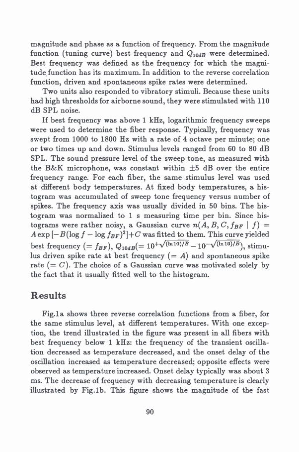
magnitude and phase as a function of frequency. From the magnitude function (tuning curve) best frequency and Q10dB were determined. Best frequency was defined as the frequency for which the magnitude.function has its maximum. In addition to the reverse correlation function, driven and spontaneous spike rates were determined.

Two units also responded to vibratory stimuli. Because these units had high thresholds for airborne sound, they were stimulated with 110 dB SPL noise.

If best frequency was above 1 kHz, logarithmic frequency sweeps were used to determine the fiber response. Typically, frequency was swept from 1000 to 1800 Hz with a rate of 4 octave per minute; one or two times up and down. Stimulus levels ranged from 60 to 80 dB SPL. The sound pressure level of the sweep tone, as measured with the B&K microphone, was constant within ±5 dB over the entire frequency range. For each fiber, the same stimulus level was used at different body temperatures. At fixed body temperatures, a histogram was accumulated of sweep tone frequency versus number of spikes. The frequency axis was usually divided in 50 bins. The histogram was normalized to 1 s measuring time per bin. Since histograms were rather noisy, a Gaussian curve n( A, B, C, !BF I f) =

A exp [-B (log f - log fBF )2 ] + C was fitted to them. This curve yielded

best frequency ( = !BF ) , Q1odB( = 1o+vf(lntO)/B - 1o-vf(Into)fB), stimulus driven spike rate at best frequency ( = A) and spontaneous spike rate { = C) . The choice of a Gaussian curve was motivated solely by the fact that it usually fitted well to the histogram.

Results

Fig.1a shows three reverse correlation functions from a fiber, for the same stimulus level, at different temperatures. With one exception, the trend illustrated in the figure was present in all fibers with best frequency below 1 kHz: the frequency of the transient oscillation decreased as temperature decreased, and the onset delay of the oscillation increased as temperature decreased; opposite effects were observed as temperature increased. Onset delay typically was about 3 ms. The decrease of frequency with decreasing temperature is clearly illustrated by Fig.1b. This figure shows the magnitude of the fast

90

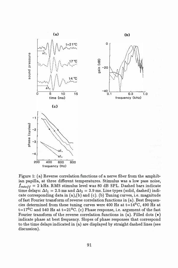
Cl) ..... :::1 Ill Ill Cl) ..... a.

"tJ c: :::1 0 Ill

....... .. Cl)

0

- 1

(a)

5 1 0 time (ms)

(c)

1 5

0 -2 >-0 ....... Cl)

� -3 .c a.

-4

200 400 600 800 frequency (Hz)

....... m "tJ .......

(b) 0

c: -20 \ "iii \ 01

-40 L--..l.---=-'":::---'-'"-:-' 0. 1 0.3 1 . 0

frequency (kHz)

Figure 1: (a) Reverse correlation functions of a nerve fiber from the amphibian papilla, at three different temperatures. Stimulus was a low pass noise, !cutoff = 2 kHz. RMS stimulus level was 80 dB SPL. Dashed bars indicate time delays: .dt1 = 2.5 ms and .dt2 = 3.9 ms. Line types (solid, dashed) indicate corresponding data in (a),(b) and (c). (b) Tuning curves, i.e. magnitude of fast Fourier transform of reverse correlation functions in (a) . Best frequencies determined from these tuning curves were 400 Hz at t=14°C, 490 Hz at t=17°C and 540 Hz at t=21°C. (c) Phase response, i.e. argument of the fast Fourier transform of the reverse correlation functions in (a). Filled dots ( • ) indicate phase at best frequency. Slopes of phase responses that correspond to the time delays indicated in (a) are displayed by straight dashed lines (see discussion) .

91

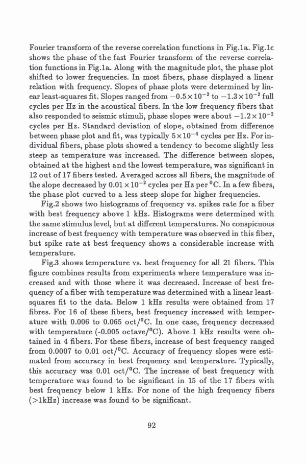
Fourier transform of the reverse correlation functions in Fig.la. Fig.lc shows the phase of the fast Fourier transform of the reverse correlation functions in Fig.la. Along with the magnitude plot, the phase plot shifted to lower frequencies. In most fibers, phase displayed a linear relation with frequency. Slopes of phase plots were determined by linear least-squares fit. Slopes ranged from -0.5 x 10-2 to -1 .3 x 10-2 full cycles per Hz in the acoustical fibers. In the low frequency fibers that also responded to seismic stimuli, phase slopes were about -1 .2 x 10-2 cycles per Hz. Standard deviation of slope, obtained from difference between phase plot and fit , was typically 5 x 10-4 cycles per Hz. For individual fibers, phase plots showed a tendency to become slightly less steep as temperature was increased. The difference between slopes, obtained at the highest and the lowest temperature, was significant in 12 out of 17 fibers tested. Averaged across all fibers, the magnitude of the slope decreased by 0.01 x 10-2 cycles per Hz per °C. In a few fibers, the phase plot curved to a less steep slope for higher frequencies.

Fig.2 shows two histograms of frequency vs. spikes rate for a fiber with best frequency above 1 kHz. Histograms were determined with the same stimulus level, but at different temperatures. No conspicuous increase of best frequency with temperature was observed in this fiber, but spike rate at best frequency shows a considerable increase with temperature.

Fig.3 shows temperature vs. best frequency for all 21 fibers. This figure combines results from experiments where temperature was increased and with those where it was decreased. Increase of best frequency of a fiber with temperature was determined with a linear leastsquares fit to the data. Below 1 kHz results were obtained from 17 fibres. For 16 of these fibers, best frequency increased with temperature with 0.006 to 0.065 oct/°C. In one case, frequency decreased with temperature ( -0.005 octaveJOC). Above 1 kHz results were obtained in 4 fibers. For these fibers, increase of best frequency ranged from 0.0007 to 0.01 oct/°C. Accuracy of frequency slopes were estimated from accuracy in best frequency and temperature. Typically, this accuracy was 0.01 octjOC. The increase of best frequency with temperature was found to be significant in 15 of the 17 fibers with best frequency below 1 kHz. For none of the high frequency fibers (>1kHz) increase was found to be significant .

92

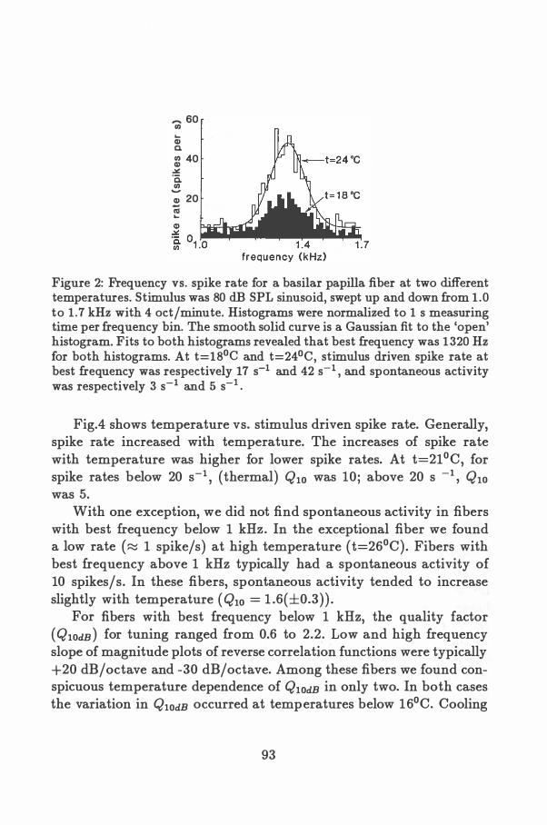
....... 60 1/) ... Q) a.

:l 40 .ll: ·c. 1/)

.....

Q) 20 iii ...

Figure 2: Frequency vs. spike rate for a basilar papilla fiber at two different temperatures. Stimulus was 80 dB SPL sinusoid, swept up and down from 1.0 to 1.7 kHz with 4 oct/minute. Histograms were normalized to 1 s measuring time per frequency bin. The smooth solid curve is a Gaussian fit to the 'open' histogram. Fits to both histograms revealed that best frequency was 1320 Hz for both histograms. At t=18°C and t=24°C, stimulus driven spike rate at best frequency was respectively 17 s-1 and 42 s-1 , and spontaneous activity was respectively 3 s-1 and 5 s-1 .

Fig.4 shows temperature vs. stimulus driven spike rate. Generally, spike rate increased with temperature. The increases of spike rate with temperature was higher for lower spike rates. At t=21 °C, for spike rates below 20 s-\ (thermal) Q10 was 10; above 20 s -1 , Q10 was 5.

With one exception, we did not find spontaneous activity in fibers with best frequency below 1 kHz. In the exceptional fiber we found a low rate (� 1 spike/s) at high temperature (t=26°C) . Fibers with best frequency above 1 kHz typically had a spontaneous activity of 10 spikes/s. In these fibers, spontaneous activity tended to increase slightly with temperature ( Q10 = 1 .6(±0.3)) .

For fibers with best frequency below 1 kHz, the quality factor ( Q1odB) for tuning ranged from 0.6 to 2.2. Low and high frequency slope of magnitude plots of reverse correlation functions were typically +20 dB/octave and -30 dB/octave. Among these fibers we found conspicuous temperature dependence of Q1odB in only two. In both cases the variation in Q1odB occurred at temperatures below 16°C. Cooling

93

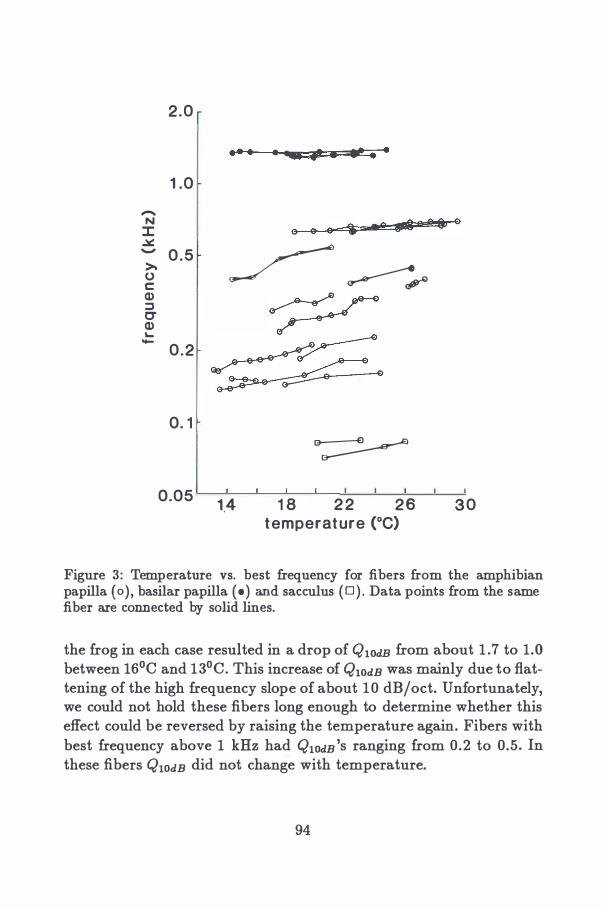
2.0

•• • . ... , • t! • •

1 .0

-N

a a--=-' ,.s 8 8 e 8 E> ::I: G

�

� - 0.5 >-

�r 0 c Q)

� ::::1 0' Q) '-

~ -

0.2

0. 1

�

0.05 1.4 1 8 2 2 2 6 3 0 temperature (°C)

Figure 3: Temperature vs. best frequency for fibers from the amphibian papilla ( o ) , basilar papilla ( •) and sacculus (D) . Data points from the same fiber are connected by solid lines.

the frog in each case resulted in a drop of Q1odB from about 1 . 7 to 1.0 between 16°C and 13°C. This increase of Q1odB was mainly due to flattening of the high frequency slope of about 10 dB/oct. Unfortunately, we could not hold these fibers long enough to determine whether this effect could be reversed by raising the temperature again. Fibers with best frequency above 1 kHz had Q10dB 's ranging from 0.2 to 0.5. In these fibers Q10dB did not change with temperature.

94

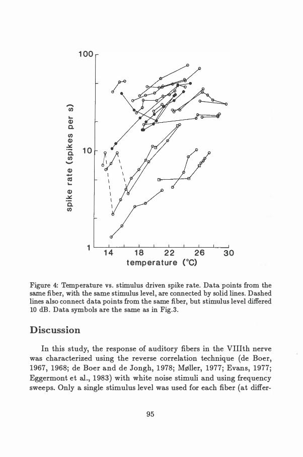
1 00

-en ... Q) c. en Q)

..ll::: 1 0 c.

!)\ en -

Q) - I m ...

Q) ..ll::: c. en

1 ��--��--��--��---L� 1 4 1 8 2 2 26 30 temperature (°C)

Figure 4: Temperature vs. stimulus driven spike rate. Data points fro� the same fiber, with the same stimulus level, are connected by solid lines. Dashed lines also connect data points from the same fiber, but stimulus level differed 10 dB. Data symbols are the same as in Fig.3.

Discussion

In this study, the response of auditory fibers in the VIIIth nerve was characterized using the reverse correlation technique (de Boer, 1967, 1968; de Boer and de Jongh, 1978; MszSller, 1977; Evans, 1977; Eggermont et al., 1983) with white noise stimuli and using frequency sweeps. Only a single stimulus level was used for each fiber (at differ-

95

ent temperatures) . This limited stimulus ensemble was used because fibers could be held for a limited time. During experiments most time was spent by changing the animals body temperature. Thus, at each temperature the fiber response had to be characterized quickly. The reverse correlation technique is very suitable for this purpose. The reverse correlation function equals the input-output correlation function of the peripheral auditory system. Input is sound pressure at the tympanic membrane and output is obtained by characterizing the spike train in an auditory nerve fiber as a train of delta-function pulses. If we model the system between tympanic membrane and auditory fiber as linear system followed by a nonlinear stochastic spike generator, and use white Gaussian noise as stimulus, then the reverse correlation function is proportional to the impulse response of the linear system. Obviously, in the ear the hypothetical linear system is a bandpass filter (de Boer, 1967, 1968; de Boer and de Jongh, 1978; Mszjller, 1977; Evans, 1977; Eggermont et al. , 1983) . By examining changes of the reverse correlation function with temperature, we focus our attention only on this linear filter. By fast Fourier transforming the reverse correlation function we can determine the amplitude and phase responses of the filter. A reverse correlation function can only be obtained for fibers that phase-lock to the stimulus (Eggermont et al., 1983) . Since fibers in the frog ear do not phase-lock to stimulus frequencies above 1 kHz (Shofner and Feng, 1981; Hillery and Narins, 1983) , we used frequency sweeps to characterize the response of fibers most sensitive to those frequencies.

Best frequency In the bullfrog inner ear, auditory fibers with best frequency above

1 kHz innervate the basilar papilla. Fibers with best frequencies below 1 kHz innervate the amphibian papilla. The sacculus is also sensitive to low frequency ( <300 Hz) airborne sound with high intensity and to seismic stimuli (Lewis et al. , 1982b ) . For fibers from the amphibian papilla and the sacculus we found that best frequency increases with temperature. Fibers from the basilar papilla (>1kHz) showed no significant increase. We do not know to what extent the different temperature effects found in fibers with best frequency above and below 1 kHz can be attributed to the different stimuli used. However,

96

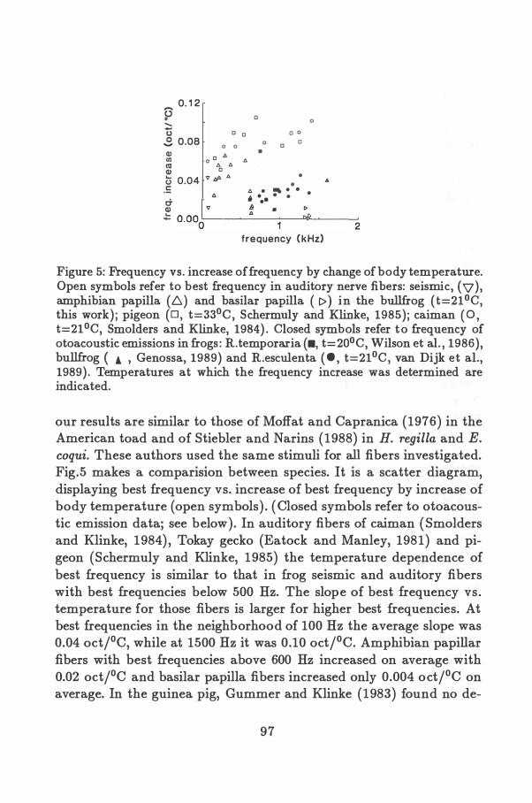
0. 1 2 ? ...... -u 0 0 � 0.08 0 0 Ql 0 I> Cll o � A

A

::: 0

l3 0.04 v do I>

0

•

0 0

0 0 0

• •

0

.= .6

A • :' : · ·

& llil • ••

Ql v � • I>

.!: 0.000�'-----�--�--�-�2 frequency (kHz)

Figure 5: Frequency vs. increase of frequency by change of body temperature. Open symbols refer to best frequency in auditory nerve fibers: seismic, (\7), amphibian papilla (.6.) and basilar papilla ( 1>) in the bullfrog (t=21°C, this work); pigeon (D, t=33°C, Schermuly and Klinke, 1985); caiman (0 , t=21°C, Smolders and Klinke, 1984) . Closed symbols refer to frequency of otoacoustic emissions in frogs: R.temporaria (•, t=20°C, Wilson et al. , 1986), bullfrog ( ! , Genossa, 1989) and R.esculenta (• , t=21°C, van Dijk et al., 1989) . Temperatures at which the frequency increase was determined are indicated.

our results are similar to those of Moffat and Capranica (1976) in the American toad and of Stiebler and Narins (1988) in H. regilla and E. coqui. These authors used the same stimuli for all fibers investigated. Fig.5 makes a comparision between species. It is a scatter diagram, displaying best frequency vs. increase of best frequency by increase of body temperature (open symbols) . (Closed symbols refer to otoacoustic emission data; see below). In auditory fibers of caiman (Smolders and Klinke, 1984) , Tokay gecko (Eatock and Manley, 1981) and pigeon (Schermuly and Klinke, 1985) the temperature dependence of best frequency is similar to that in frog seismic and auditory fibers with best frequencies below 500 Hz. The slope of best frequency vs. temperature for those fibers is larger for higher best frequencies. At best frequencies in the neighborhood of 100 Hz the average slope was 0.04 oct/°C, while at 1500 Hz it was 0.10 oct/°C. Amphibian papillar fibers with best frequencies above 600 Hz increased on average with 0.02 oct/°C and basilar papilla fibers increased only 0.004 oct/°C on average. In the guinea pig, Gummer and Klinke (1983) found no de-

97

pendence of best frequency on temperature. Several authors (Eatock and Manley, 1981; Gummer and Klinke, 1983; Smolders and Klinke, 1984; Schermuly and Klinke, 1985; Oldfield, 1988) have pointed out that differences in temperature dependence of best frequency could indicate the presence of different tuning mechanisms in different hearing organs. Thus, the mammalian cochlea and the anuran basilar papilla may use a tuning mechanisms that is different from that used by the reptilian ear, the bird ear and amphibian papilla and (evidently) the sacculus in the anuran ear.

Within the amphibian papilla the temperature experiments indicate two populations of fibers, possibly using different tuning mechanisms. For fibers with best frequencies below 600 Hz (at t=21 °0) the slopes of best frequency vs. temperature ranged up to 0.06 oct/00; above 600 Hz the slope was less than 0.03 oct/00. Our data are insufficient to decide whether the change at 600 Hz is really a discontinuity.

Additional physiological evidence for two populations of fibers in the amphibian papilla exists. Fibers with best frequency below 550 Hz exhibit two- tone suppression and response to the quadratic distortion tone f1 - f2 (Feng et al. , 1975; Capranica and Moffat, 1980) . Above 550 Hz they do not. Thus, there is a correlation between the nonlinear response properties and temperature dependence of best frequency, indicating that frequency tuning and nonlinear response may be closely linked. This correlation extends towards the basilar papilla, which shows no two-tone suppression (Feng et al. , 1975) and small (if any) temperature dependence of best frequency. Capranica and Moffat suggested that the lack of two-tone suppression above 550 Hz in the amphibian papilla is merely a consequence of the fact that the best suppressing tone would have been outside the sensitivity region of the papilla. A suppressing tone would thus apparently not be able to reach the sensory epithelium. Our data suggest a more profound difference between the operation associated with fibers with best frequencies above and below 550 Hz.

There is also morphological evidence for two populations in the amphibian papilla. Since the papilla is tonotopically organized (Lewis et al. , 1982b ) , fibers with best frequency below and above 550 Hz innervate different parts of the papilla. These two regions lie approximately on different sides of the tectorial curtain spanning the chamber

98

in which the papilla is located (the curtain is part of the tectorium covering all hair cells in the papilla, Lewis et al. , 1982b ). Hair cell orientation differs on the two sides of the curtain. Rostral to the curtain hair cells (sensitive to frequencies below 500 Hz) are orientated parallel to the length of the papilla. On the other side of the curtain, hair cell orientation is perpendicular to the long axis of the papilla. Thus, the amphibian papilla is divisible into two regions on bases of hair cell orientation, temperature dependence of best frequency, and nonlinear response properties. In each case, the dividing line occurs where best frequencies fall in the 500 to 600 Hz range.

In Fig.5 the increase of frog emission frequency with temperature is also indicated (closed symbols) . Emission data were taken from Wilson et al. (1986), Genossa (1989) and Van Dijk et al. (1989). The emission results range from 600 Hz to 1600 Hz. Generation of otoacoustic emissions is assumed to be related to frequency tuning mechanisms in the ear. In humans a close relation between minima in pure tone threshold audiogram and emission frequencies supports this view (Schloth, 1983; Long and Tubis, 1988; Horst et al., 1983). More evidence is supplied by the similar shape of neural tuning curves and iso-suppression tuning curves resulting from suppression of a emission by a pure-tone stimulus (Kemp, 1979; Wilson, 1980; Wit et al. , 1981 ; Schloth and Zwicker, 1983; Ziss and Glattke, 1988). Thus, since frequency tuning and otoacoustic emissions seem to be related, one would expect best frequency of nerve fibers and emission frequency to change with temperature in a similar way (i.e. with equal slopes) . Below 600 Hz no emission data are available. The fact that only few emissions are found below 600 Hz could be due to reduced sensitivity of the microphone used in emission experiments (van Dijk et al. , 1989). However, it could also be related to the duality of function and morphology of the amphibian papilla discussed above. For frequencies in the sensitivity range of the amphibian papilla above 600 Hz (see Fig.5) slopes of best frequency vs. temperature and those of emission frequency vs. temperature are comparable. However, in the frequency range of the basilar papilla (1 to 2 kHz), the slopes of emission frequencies are significantly greater than those of best frequencies. This is also true within the same frog species (open and closed triangles are bullfrog results) and can thus not be attributed to species differences

99

of the sensitivity ranges of both papillae. Therefore, the hypothesis that the mechanisms that determine fiber frequency tuning and emission frequency are closely related, is not supported by the temperature experiments.

QlodB We did not observe a conspicuous dependence of Q1odB on tem

perature, except in two fibers at low temperature. Also in reptilians, birds and mammals Q1odB did not change with temperature (Smolders and Klinke, 1984; Schermuly and Klinke, 1985; Gummer and Klinke, 1983) . Thus, this seems to be a property present in all species. However, some caution should be taken in comparing our Q1odB to those from other reports . Usually, Q10dB is defined as !BF/ 6.f10dB where 6.f10dB is the width of a threshold tuning curve. We defined 6.ftodB from a iso-intensity response histogram ( > 1kHz) or a reverse correlation function ( < 1kHz) . The fast Fourier transform of a reverse correlation is also best interpreted as an iso-intensity response curve (Eggermont et al. , 1983). From macro electrode recordings from the torus semicircularis in frogs, it is known that auditory threshold increases as temperature decreases (Hubl et al. , 1977; Hubl and Schneider, 1979; Mohneke and Schneider, 1979; Walkowiak, 1980). Thus, when the frog is cooled while the stimulus level is kept constant , the stimulus approaches threshold. Using the reverse correlation technique, M!1Sller (1977) found that in the rat ear tuning sharpened as the noise stimulus was lowered. This effect occurred also at levels only just above threshold. In cat (de Boer and de Jongh, 1978; Evans, 1977), however, the reverse correlation function did not change much until the stimulus was taken up to 45 dB above threshold, although there is prominent nonlinear response to tonal stimuli (Sachs and Kiang, 1968). Thus, although the auditory system is known to respond highly nonlinearly to tonal stimuli, its response to noise can be fairly linear. In the frog no data are available on linearity of neural response to noise stimuli. If, for example, in the frog lowering of the noise stimulus down to threshold turns out to narrow the tuning, then our results could mean that a Q10dB defined from a threshold tuning curve will increase as temperature increases. This would then be different from result in reptiles, birds and mammals.

100

Spike rates Although the tuning characteristics of seismic (presumably sac

cular) fibers, amphibian papilla fibers and basilar papilla fibers show a certain variety in their dependence on temperature, the stimulus driven spike rate behaves in the same way in all three organs as temperature is changed: iso-intensity spike rate increases with temperature. Macro electrode recordings from the torus semicircularis in several frog species (Hubl et al. , 1977; Hubl and Schneider, 1979; Mohneke and Schneider, 1979; Walkowiak, 1980) , have shown that threshold decreases as temperature increases. A threshold shift was also found by Moffat and Capranica (1976) in single fiber recordings in the American toad, although threshold in basilar papilla fibers changed only a little. However, the macro electrode torus recordings show that temperature change of threshold in the frequency range of the basilar papilla varies considerably among species. We did not determine threshold, but determined spike rate in response to a :fixedRMS-amplitude stimulus. Increase of spike rate with constant stimulus level could be due to (1 ) decrease of threshold, (2) reduction of refractory period (as reflected in an increase of maximum firing rate) , or (3) a combination of (1 ) and (2) . Our observation that spike rates in amphibian and basilar papilla show the same temperature dependence thus is consistent with American toad results: with increasing temperature Moffat and Capranica report (1 ) decrease of threshold and approximately constant dynamic range for amphibian papilla fibers, and (2) little change of threshold but increase of maximum firing rate for basilar papilla fibers.

The torus semicircularis recordings indicate that hearing threshold in a given frog species is optimal at temperatures at which the species usually mates. Thus, the ear is designed in a way which optimizes the chance for a frog to get in contact with a mating partner. For the bullfrog this preferred mating temperature apparently is in the 20°C's (Duellman and Trueb, 1986) . We found higher spike rate in the 20°C's as compared to the 10°C's. This could be due to decrease of threshold. Although we did not take temperature high enough to reveal an optimum, our result would then be in agreement with the finding that the sensitivity of the hearing organ of a frog species is optimal at temperatures at which the species usually searches for a

101

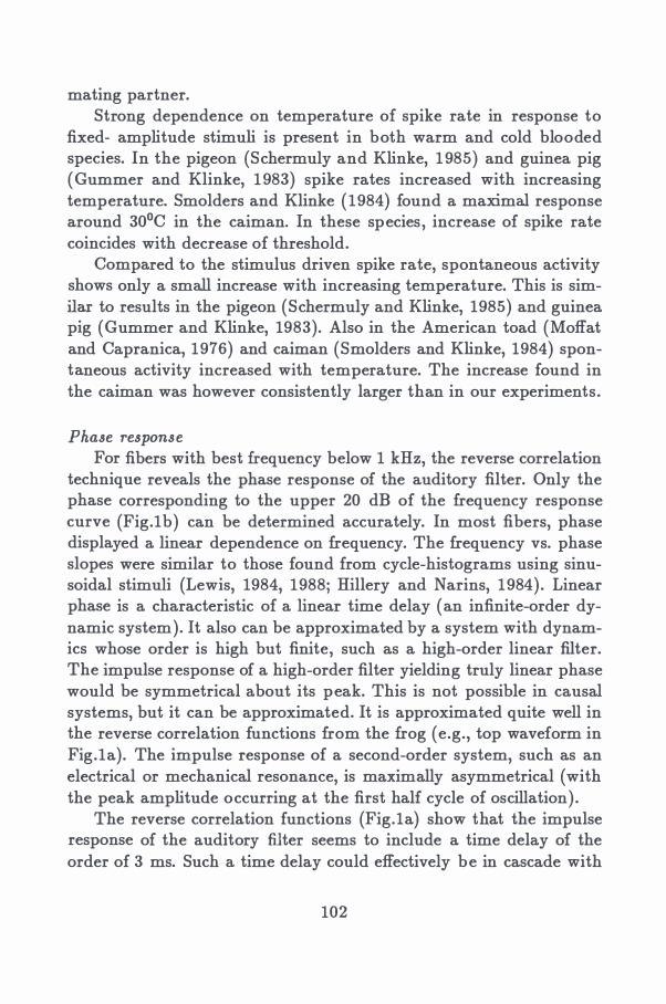
mating partner. Strong dependence on temperature of spike rate in response to

fixed- amplitude stimuli is present in both warm and cold blooded species. In the pigeon (Schermuly and Klinke, 1985) and guinea pig ( Gummer and Klinke, 1983) spike rates increased with increasing temperature. Smolders and Klinke (1984) found a maximal response around 30°C in the caiman. In these species, increase of spike rate coincides with decrease of threshold.

Compared to the stimulus driven spike rate, spontaneous activity shows only a small increase with increasing temperature. This is similar to results in the pigeon (Schermuly and Klinke, 1985) and guinea pig (Gummer and Klinke, 1983). Also in the American toad (Moffat and Capranica, 1976) and caiman (Smolders and Klinke, 1984) spontaneous activity increased with temperature. The increase found in the caiman was however consistently larger than in our experiments.

Phase response For fibers with best frequency below 1 kHz, the reverse correlation

technique reveals the phase response of the auditory filter. Only the phase corresponding to the upper 20 dB of the frequency response curve (Fig.1b) can be determined accurately. In most fibers, phase displayed a linear dependence on frequency. The frequency vs. phase slopes were similar to those found from cycle-histograms using sinusoidal stimuli (Lewis, 1984, 1988; Hillery and Narins, 1984) . Linear phase is a characteristic of a linear time delay (an infinite-order dynamic system). It also can be approximated by a system with dynamics whose order is high but finite, such as a high-order linear filter. The impulse response of a high-order filter yielding truly linear phase would be symmetrical about its peak. This is not possible in causal systems, but it can be approximated. It is approximated quite well in the reverse correlation functions from the frog (e.g., top waveform in Fig.1a). The impulse response of a second-order system, such as an electrical or mechanical resonance, is maximally asymmetrical (with the peak amplitude occurring at the first half cycle of oscillation) .

The reverse correlation functions (Fig.la) show that the impulse response of the auditory filter seems to include a time delay of the order of 3 ms. Such a time delay could effectively be in cascade with

102

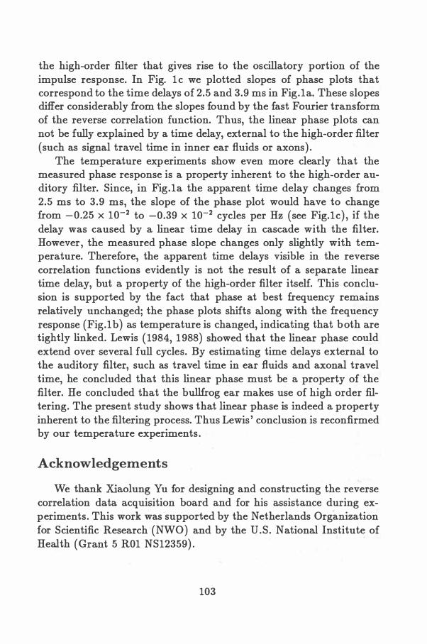
the high-order filter that gives rise to the oscillatory portion of the impulse response. In Fig. 1c we plotted slopes of phase plots that correspond to the time delays of 2.5 and 3.9 ms in Fig.1a. These slopes differ considerably from the slopes found by the fast Fourier transform of the reverse correlation function. Thus, the linear phase plots can not be fully explained by a time delay, external to the high-order filter (such as signal travel time in inner ear fluids or axons) .

The temperature experiments show even more clearly that the measured phase response is a property inherent to the high-order auditory filter. Since, in Fig.1a the apparent time delay changes from 2.5 ms to 3.9 ms, the slope of the phase plot would have to change from -0.25 x 10-2 to -0.39 x 10-2 cycles per Hz (see Fig.1c) , if the delay was caused by a linear time delay in cascade with the filter. However, the measured phase slope changes only slightly with temperature. Therefore, the apparent time delays visible in the reverse correlation functions evidently is not the result of a separate linear time delay, but a property of the high-order filter itself. This conclusion is supported by the fact that phase at best frequency remains relatively unchanged; the phase plots shifts along with the frequency response (Fig.1b) as temperature is changed, indicating that both are tightly linked. Lewis (1984, 1988) showed that the linear phase could extend over several full cycles. By estimating time delays external to the auditory filter, such as travel time in ear fluids and axonal travel time, he concluded that this linear phase must be a property of the filter. He concluded that the bullfrog ear makes use of high order filtering. The present study shows that linear phase is indeed a property inherent to the filtering process. Thus Lewis ' conclusion is reconfirmed by our temperature experiments .

Acknowledgements

We thank Xiaolung Yu for designing and constructing the reverse correlation data acquisition board and for his assistance during experiments. This work was supported by the Netherlands Organization for Scientific Research (NWO) and by the U.S. National Institute of Health (Grant 5 R01 NS12359) .

103

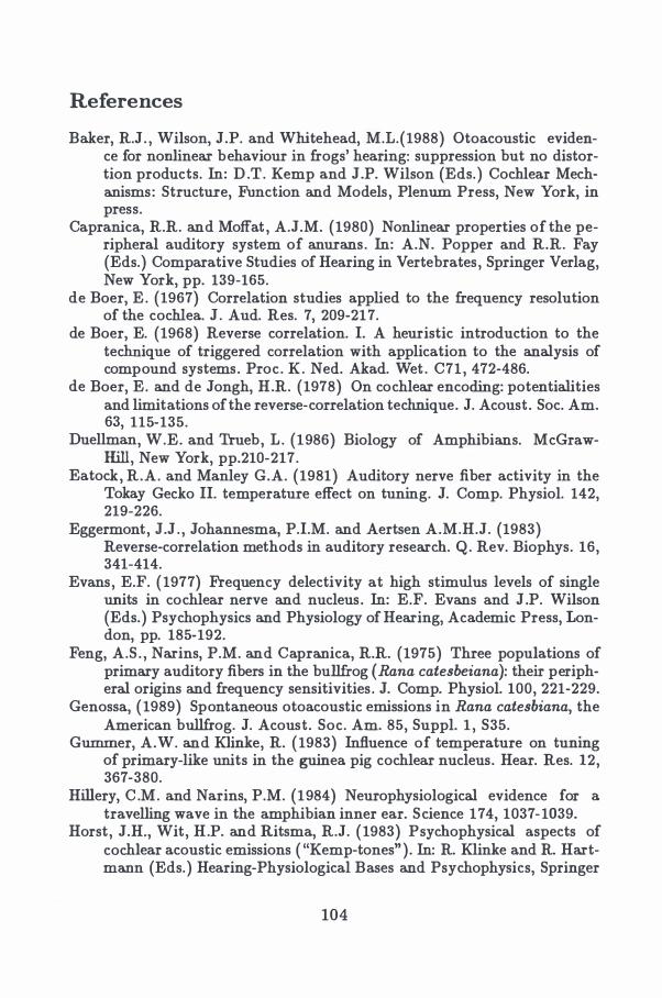
References

Baker, R.J. , Wilson, J.P. and Whitehead, M.L.(1988) Otoacoustic evidence for nonlinear behaviour in frogs' hearing: suppression but no distortion products. In: D .T. Kemp and J.P. Wilson (Eds.) Cochlear Mechanisms: Structure, Function and Models, Plenum Press, New York, in press.

Capranica, R.R. and Moffat , A.J.M. (1980) Nonlinear properties of the peripheral auditory system of anurans. In: A.N. Popper and R.R. Fay (Eds.) Comparative Studies of Hearing in Vertebrates, Springer Verlag, New York, pp. 139-165.

de Boer, E. (1967) Correlation studies applied to the frequency resolution of the cochlea. J . Aud. Res. 7, 209-217.

de Boer, E. (1968) Reverse correlation. I. A heuristic introduction to the technique of triggered correlation with application to the analysis of compound systems. Proc. K . Ned. Akad. Wet . C71 , 472-486.

de Boer, E. and de Jongh, H.R. (1978) On cochlear encoding: potentialities and limitations of the reverse-correlation technique. J. Acoust. Soc. Am. 63, 115-135.

Duellman, W.E. and Trueb, L . (1986) Biology of Amphibians. McGrawHill, New York, pp.210-217. Eatock, R.A. and Manley G.A. (1981) Auditory nerve fiber activity in the

Tokay Gecko II. temperature effect on tuning. J. Camp. Physiol. 142, 219-226.

Eggermont, J.J . , Johannesma, P.I.M. and Aertsen A.M.H.J. (1983) Reverse-correlation methods in auditory research. Q . Rev. Biophys. 16, 341-414.

Evans, E.F. (1977) Frequency delectivity at high stimulus levels of single units in cochlear nerve and nucleus. In: E.F. Evans and J .P. Wilson (Eds.) Psychophysics and Physiology of Hearing, Academic Press, London, pp. 185-192.

Feng, A.S . , Narins, P.M. and Capranica, R.R. (1975) Three populations of primary auditory fibers in the bullfrog (Rana catesbeiana): their peripheral origins and frequency sensitivities . J. Camp. Physiol. 100, 221-229.

Genossa, (1989) Spontaneous otoacoustic emissions in Rana catesbiana, the American bullfrog. J. Acoust. Soc. Am. 85, Suppl. 1 , S35.

Gummer, A.W. and Klinke, R. (1983) Influence of temperature on tuning of primary-like units in the guinea pig cochlear nucleus. Hear. Res. 12, 367-380.

Hillery, C .M. and Narins, P.M. (1984) Neurophysiological evidence for a travelling wave in the amphibian inner ear. Science 174, 1037-1039.

Horst , J.H., Wit, H.P. and Ritsma, R.J. (1983) Psychophysical aspects of cochlear acoustic emissions ( "Kemp-tones" ) . In: R. Klinke and R. Hartmann (Eds.) Hearing-Physiological Bases and Psychophysics, Springer

104

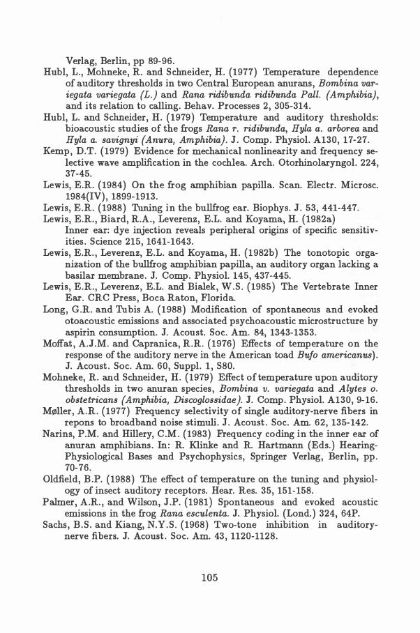
Verlag, Berlin, pp 89-96. Hubl, L., Mohneke, R. and Schneider, H. (1977) Temperature dependence

of auditory thresholds in two Central European anurans, Bombina variegata variegata (L.) and Rana ridibunda ridibunda Pall. {Amphibia), and its relation to calling. Behav. Processes 2, 305-314.

Hubl, L. and Schneider, H. (1979 ) Temperature and auditory thresholds: bioacoustic studies of the frogs Rana r. ridibunda, Hyla a. arborea and Hyla a. savignyi {Anura, Amphibia). J. Comp. Physiol. A130, 17-27.

Kemp, D.T. (1979) Evidence for mechanical nonlinearity and frequency selective wave amplification in the cochlea. Arch. Otorhinolaryngol. 224, 37-45.

Lewis, E.R. (1984) On the frog amphibian papilla. Scan. Electr. Microsc. 1984(IV) , 1899-1913.

Lewis, E.R. (1988) Tuning in the bullfrog ear. Biophys. J. 53, 441-447. Lewis, E.R. , Biard, R.A., Leverenz, E.L. and Koyama, H. (1982a)

Inner ear: dye injection reveals peripheral origins of specific sensitivities . Science 215, 1641-1643.

Lewis, E.R. , Leverenz, E.L. and Koyama, H. (1982b) The tonotopic organization of the bullfrog amphibian papilla, an auditory organ lacking a basilar membrane. J. Comp. Physiol. 145, 437-445.

Lewis, E.R., Leverenz, E.L. and Bialek, W.S. (1985) The Vertebrate Inner Ear. CRC Press , Boca Raton, Florida.

Long, G.R. and Tubis A. (1988) Modification of spontaneous and evoked otoacoustic emissions and associated psychoacoustic microstructure by aspirin consumption. J. Acoust. Soc. Am. 84, 1343-1353.

Moffat , A.J.M. and Capranica, R.R. (1976) Effects of temperature on the response of the auditory nerve in the American toad Bufo americanus) . J. Acoust . Soc. Am. 60, Suppl. 1 , S80.

Mohneke, R. and Schneider, H. (1979) Effect of temperature upon auditory thresholds in two anuran species , Bombina v. variegata and Alytes o. obstetricans (Amphibia, Discoglossidae). J. Comp. Physiol. A130, 9-16.

M!1)ller, A.R. (1977) Frequency selectivity of single auditory-nerve fibers in repons to broadband noise stimuli. J. Acoust . Soc. Am. 62, 135-142.

Narins, P.M. and Hillery, C .M. (1983) Frequency coding in the inner ear of anuran amphibians. In: R. Klinke and R. Hartmann (Eds.) HearingPhysiological Bases and Psychophysics, Springer Verlag, Berlin, pp. 70-76.

Oldfield, B .P. (1988) The effect of temperature on the tuning and physiology of insect auditory receptors. Hear. Res. 35, 151-158.

Palmer, A.R. , and Wilson, J.P. (1981 ) Spontaneous and evoked acoustic emissions in the frog Rana esculenta. J. Physiol. (Lond.) 324, 64P.

Sachs, B.S . and Kiang, N.Y.S . (1968) Two-tone inhibition in auditorynerve fibers. J. Acoust . Soc. Am. 43, 1120-1128.

105

Schermuly, L. and Klinke, R. (1985) Change of characteristic frequency of pigeon primary auditory afferents with temperature. J. Comp. Physiol. 156, 209-211 .

Schloth, E . (1983) Relation between spectral composition of spontaneous otoacoustic emissions and fine-structure of threshold in quiet. Acustica 53, 250-256.

Schloth, E. and Zwicker, E. (1983) Mechanical and acoustical influences of spontaneous oto-acoustic emissions. Hear. Res. 11 , 285-293.

Shofner, W.P. and Feng, A.S. (1981) Post-metamorphic development of the frequency selectivities and sensitivities of the peripheral auditory system of the bullfrog, Rana catesbeiana. J. Exp. Biol. 93, 181-196.

Smolders, J.W.T. and Klinke, R. (1984) Effects of temperature on the properties of primary auditory fibres of the spectacled caiman, Caiman crocodilus (L.). J. Comp. Physiol. A155, 19- 30.

Stiebler, I. and Narins, P.M. (1988) personal communication. van Dijk, P. and Wit, H.P. (1987) Temperature dependence of frog sponta

neous otoacoustic emissions. J. Acoust. Soc. Am. 82, 2147-2150. van Dijk, P. , Wit , H.P. and Segenhout , J.M. (1989) Spontaneous otoacous

tic emissions in the European edible frog (Rana esculenta): Spectral details and temperature dependence. Chapter 3 of this thesis, and Hear. Res. , accepted.

Walkowiak, W. (1980) Sensitivity, range and temperature dependence of hearing in the grass frog and fire-bellied toad. Behav. Processes 5, 363-372.

Wilson, J.P. (1980) Evidence for a cochlear origin for acoustical re-emission, threshold fine-structure and tonal tinnitus. Hear. Res. 2 , 233-252.

Wilson, J.P. , Whitehead, M.L. and Baker, R.J. 1986 The effect of temperature on otoacoustic emission tuning properties . In: B.C.J. Moore and R.D Patterson (Eds. ) , Auditory Frequency Selectivity, Plenum Press, London, pp.39-46.

Wit, H.P. , Langevoort , J.C. and Ritsma, R.J. (1981) Frequency spectra of cochlear acoustic emissions ( 'Kemp-echoes') . J. Acoust . Soc. Am. 70, 437-445.

Ziss, C .A. and Glattke, T .J. (1988) Reliability of spontaneous otoacoustic emission suppression tuning curve measures. J. Sp. Hear. Res. 31, 616-619.

106

SAMENVATTING

Eigenschappen en mechanismen van spontane otoakoestische emissies

Dit proefschrift beschrijft spontane otoakoestische ermsstes van mensen en kikkers. Met een gevoelige microfoon, aangesloten op een oor van b.v. een mens, kunnen in veel gevallen zachte fluittoontjes worden geregistreerd. De frequenties van deze spontane otoakoestische emissies liggen doorgaans tussen de 1 en 3 kHz, terwijl het geluidsniveau van emissies rond de gehoordrempel ligt . De meest gangbare opvatting over het ontstaan van een emissie is, dat deze gegenereerd wordt door een actief auditief filter. Instabiliteit van een dergelijk :filter zou de oorzaak zijn van een mechanische oscillatie in het binnenoor, die een akoestische emissie in de gehoorgang tot gevolg heeft .

Hoofdstuk 1 behandelt synchronisatie van spontane otoakoestische emissies. Synchronisatie is karakteristiek voor de interactie tussen een oscillator en een periodieke kracht (stimulus). Deze interactie wordt gekenmerkt door een strijd tussen de oscillator, die zijn eigen frequentie /0 in stand probeert te houden, en de kracht, die zijn frequentie /. probeert op te dringen aan de oscillator.

Synchronisatie van spontane otoakoestische emissies kan bestudeerd worden door een toon met frequentie f. als stimulus aan te bieden aan een oor, dat een emissie met frequentie /0 genereert. Als de stimulus voldoende sterk is, zal de emissiefrequentie verschuiven naar de synchronisatiefrequentie f • . Een nadeel van een dergelijke aanpak is, dat emissie en stimulus (beide aanwezig in de gehoorgang) niet van elkaar gescheiden kunnen worden; b. v. door :filtering van het microfoonsignaal. Daarom werd als synchroniserende periodieke 'kracht '

107

een toon gebruikt die in het oor werd opgewekt. Dit gebeurde met een stimulus bestaande uit twee tonen met respectievelijk de frequenties f1 en f2 • Een dergelijke stimulus genereert in het oor een kombinatietoon met frequentie f. = 2ft - f2 • De frequenties f1 en f2 werden zo gekozen dat fa dicht bij de emissiefrequentie fo lag. Omdat de stimulusfrequenties f1 en f2 aanzienlijk verschillen ("' 200 Hz) van de emissiefrequentie fo en de synchronisatiefrequentie fa , kan nu door filtering van het i:nicrofoonsignaal de emissie gescheiden worden van de stimulus. Aan de hand van het gefilterde microfoonsignaal kan synchronisatie van de emissie in detail worden bestudeerd.

In Hoofdstuk 1 wordt vooral de analyse van de fase van een emissie t .o.v. de kombinatietoon met frequentie f. uitgebreid beschreven. Bij deze analyse werd gebruik gemaakt van registratie van nuldoorgangen van het gefilterde microfoonsignaal. Bij voldoende intensiteit ( "' 30 dB SPL) van de primaire tonen f1 en f2 , fl.uctueerde de emissiefase rond een constante waarde: de in het oor opgewekte kombinatietoon was voldoende sterk om de emissie te synchroniseren met frequentie fa· Als de primaire tonen zachter waren ("' 20 dB SPL ), bleken op ongeregelde momenten 21r-fasesprongen op te treden: af en toe ontglipt de emissie aan synchronisatie, om zijn eigen frequentie fo te herstellen. Blijkbaar was de kombinatietoon dan niet voldoende sterk om de emissie voortdurend te synchroniseren.

De interactie van een emissie met een kubisch vervormingsprodukt, zoals beschreven in Hoofdstuk 1 , is analoog aan de interactie tussen een oscillator en een periodieke kracht. De onregelmatigheid van de fasesprongen kan verklaard worden, door aan te nemen dat de emissieoscillator in kontakt staat met een ruisbron (b.v. thermische ruis) .

Hoofdstuk 2 beschrijft de analyse van amplitude- en frequentiefl.uctuaties van spontane otoakoestische emissies . Een emissiesignaal kan beschreven worden als een harmonische trilling waarvan de amplitude en de frequentie fl.uctueren. Zoals al werd vermeld, kan een oor soms meerdere emissies met verschillende frequentie en luidheid uitzenden. Per oor (8 mensen- en 2 kikkeroren) werd voor de luidste emissie het amplitudesignaal A(t) en de periode T(ti ) bepaald. De peri ode ( = inverse van de frequentie) werd bepaald door de tijd tussen opeenvolgende nuldoorgangen ti-l en ti te meten. Bij mensen bleek, dat respectievelijk amplitude en periode gemiddeld slechts

108

3% en 0.07% :fluctueerden. Voor beide kikkeremissies waren de fluctuaties ongeveer 10 keer zo groot. N aast dit verschil tussen emissies bij kikkers en mensen, werden voornamelijk overeenkomsten gevonden: (1) De verhouding tussen de grootte van respectievelijk amplitude- en frequentiefluctuaties lag in de zelfde orde van grootte voor alle onderzochte emissies. (2) Uit spectra van A(t) en T(ti) bleek dat amplitude en frequentie langzaam fluctueren t.o.v. de frequentie van de emissie: de afsnijfrequentie van deze spectra was in de orde van 10 Hz.

N aast de experimentele resultaten beschrijft Hoofdstuk 2 amplitude- en frequentiefluctuaties van een mathematische oscillator. Deze beschrijving spitst zich toe op de vraag "wat kan men over de oscillator te weten komen door bestudering van amplitude- en frequentiefluctuaties?" In het model worden de :fluctuaties veroorzaakt door wisselwerking van de oscillator met een ruisbron. Omdat zowel de amplitude- als de frequentiefluctuaties veroorzaakt worden door dezelfde ruisbron, zal er een verband tussen beide fluctuaties bestaan. De wijze waarop amplitude- en frequentiefluctuaties verband houden is echter verschillend voor verschillende types oscillatoren en ruisbronnen. Bestudering van de fluctuaties kan dus inderdaad informatie opleveren over de oscillator, maar ook over de ruisbron.

Omdat de oscillator, waardoor een spontane otoakoestische emissie wordt gegenereerd, zich bevindt in het binnenoor van b.v. een mens, hebben we geen direkte toegang tot die oscillator. Daarom vormt bestudering van amplitude- en frequentiefluctuaties van emissiesignalen een mogelijkheid om de eigenschappen van de emissiegenerator te onderzoeken. Uit vergelijking van de experimentele met de theoretische resultaten blijkt , dat een oscillator met lineaire stijfheid (b.v. een Van der Pol oscillator), die aangedreven wordt met witte Gaussische ruis, niet afdoende de emissiegenerator kan beschrijven. Andere oscillatoren (b.v. met niet-lineaire stijfheid) en ruisbronnen (b.v. smalbandige ruis ) , die mogelijk wei de experimentele resultaten kunnen verklaren, worden in Hoofdstuk 2 besproken.

Hoofdstuk 3 is in zijn geheel gewijd aan spontane otoakoestische emissies van kikkers (Rana esculenta) . Spontane emissies werden gevonden in 71% van de onderzochte kikkeroren. Van alle tot nu toe onderzochte diersoorten blijken alleen de kikker en de mens (30%) frequent spontane emissies te genereren. In vergelijking met mensen

109

hehhen kikkers een eenvoudig hinnenoor. Blijkhaar is de complexe structuur van het mensenoor niet nodig om emissies op te wekken.

De frequentie van de geregistreerde kikkeremissies lag tussen 450 en 1350 Hz. Deze frequenties zijn verdeeld over twee gescheiden populaties: een hoven en een heneden 1 kHz. Met een uitzondering traden hooguit twee emissies op in elk kikkeroor. Als twee emissies werden gevonden, lag er een hoven en een heneden 1 kHz. Dit is opmerkelijk, omdat de twee gehoororgaantjes (de amfihische en de hasilaire papilla) in het oor van de kikker Rana esculenta waarschijnlijk gevoelig zijn voor geluiden met frequenties resp. heneden en hoven ongeveer 1 kHz.

Een emissiesignaal V(t), dat geregistreerd werd in een kikkeroor, werd gedigitaliseerd tot een signaal Vi. Van de get allen Vi werd een histogram P (Vi) hepaald. De vorm van P (Vi) is gelijk aan die van de waarschijnlijkheidsverdeling van een sinusvormig signaal waaraan ruis is toegevoegd. Daarom is geconcludeerd dat, evenals emissies van mensen, ook emissies van kikkers gegenereerd worden door een actieve oscillator.

Omdat kikkers koudhloedig zijn, past de lichaamstemperatuur van een kikker zich aan hij de omgevingstemperatuur. In 4 kikkers werd de invloed van lichaamstemperatuur op de intensiteit en de frequentie van emissies onderzocht. Een emissie kon worden "in- of uitgeschakeld" door de temperatuur een paar graden te veranderen. Bij temperaturen heneden het "schakelinterval" was de emissie "uitgeschakeld" ; hij hogere temperaturen, waarvoor de emissie was "ingeschakeld" , werd geen duidelijk verhand tussen temperatuur en emissieintensiteit gevonden. De frequentie van een emissie nam hij stijgende temperatuur toe (met 0.02 tot 0.04 octaaf per graad Celcius)

Hoofdstuk 4 heschrijft de temperatuurafhankelijkheid van neurale responsies in auditieve zenuwvezels van de Amerikaanse hrulkikker (Rana catesbeiana). Stijgende en dalende temperatuur hadden een reversihel effect. Temperatuurstijging resulteerde in toename van zg. heste frequentie (/BF) van zenuwvezels die in kontakt staan met de amfihische papilla (/BF < 1 kHz; toenamen tot 0.06 octjOC) . In zenuwvezels van de hasilaire papilla (/BF > 1 kHz) werd geen significante toename van de heste frequentie waargenomen. Dit hetekent dat hoven 1 kHz de heste frequentie van auditieve zenuwvezels en

110

de emissiefrequentie (zie Hoofdstuk 3) een verschillende temperatuurcoefficient hebben. De beste frequentie van een zenuwvezel en de emissiefrequentie worden dus niet bepaald door hetzelfde afstemmechanisme. Vergelijking van de resultaten in de Hoofdstukken 3 en 4 levert dus geen ondersteuning op voor de hypothese, dat emissiegeneratie en frequentieselectiviteit van zenuwvezels door dezelfde auditieve filters worden veroorzaakt.

111

N AWOORD

De tekst op de voorkant van dit proefschrift doet vermoeden dat de totstandkoming ervan een eenmansoperatie was. Niets is echter minder waar. Een aantal personen heeft een onmisbare bijdrage geleverd aan dit proefschrift:

In de eerste plaats gaat mijn dank uit naar HERO WIT . Hero, aan jou heb ik een ideale promotor gehad. Je hebt mij gedurende 4 jaar met zeer fijn afgemeten doseringen bekend gemaakt met de wereld van het gehoor. De dagelijkse discussies die wij voerden waren van onschat bare waarde voor het verloop van het onderzoek. Het persoonlijke kontakt met jou zal ik niet vergeten. Ik wens jou nog vele promovendi toe, en ik wens vele promovendi jou als promotor toe.

DIEK DUIFHUIS, jij hebt mijn promotieonderzoek van iets grotere afstand meegemaakt . Jouw warme belangstelling is echter een grote stimulans geweest tijdens de afgelopen 4 jaar. En hoe je het voor elkaar krijgt weet ik niet, maar een enkele vraag van jou kon me soms voor weken aan het denken zetten.

HANS SEGENHOUT, jouw kundigheid en kreativiteit hebben een grote rol gespeeld bij het onderzoek dat ten grondslag ligt aan Hoofdstuk 3 van dit proefschrift. JAN VAN DIJK , aan jou heb ik een waardige Computergoeroe gehad. Aan mijn nieuwe werkkring kun je zien wat een goeroe voor zijn leerlingen betekenen kan. MEINDERT GOSLINGA

verrichtte veel foto- en diawerk. BARBARA WYNBERG-WILLIAMS gaf talrijke suggesties ten aanzien van het 'Engels' in dit proefschrift. ALJA MENSINK adviseerde met betrekking tot de vormgeving.

TED LEWIS AND CO- WORKERS, I thank you for the hospitality I enjoyed in your lab. Your impressive expertise gave birth to Chapter 4 of this thesis. I will not forget the wonderful time I had in Berkeley.

Uiteraard was dit proefschrift onmogelijk geweest zonder de

113

PROEFPERSONEN. Hen dank ik voor het geduldig eindeloos stilliggen. De bovengenoemde mensen hebben ieder een bijdrage geleverd aan

de inhoud van dit proefschrift . Dat het af is, is mooi. Maar nog veel belangrijker vind ik het vier jaar bijzonder plezierig gewerkt te hebben. Daarvoor bedank ik aile MEDEWERKERS VAN RET AUDIOLOGISCH INSTITUUT.

En tot slot, JACQUELINE. Helaas had je geen emissies. Toch ben jij voor mij een constante bron van energie.

Pim van Dijk

114

characteristics and mechanisms emissions

Documents