Correlation, Reliability and Regression

Chapter 7

Correlation Statistic that describes the relationship

between scores (Pearson r). Number is the correlation coefficient. Ranges between +1.00 and –1.00. Positive is direct relationship. Negative is inverse relationship. .00 is no relationship. Does not mean cause and effect. Measured by a Z score. Generally looking for scores greater than .5

Reliability

Statistic used to determine repeatabilityNumber ranges between 0 and 1Always positiveCloser to one is greater reliabilityCloser to 0 is less reliabilityGenerally looking for values greater

than .8

Scattergram or ScatterplotDesignate one variable X and one Y.Draw and label axes.Lowest scores are bottom left.Plot each pair of scores.Positive means high on both scores.Negative means high on one and low on

the other. IQ and GPA? ~ 0.68

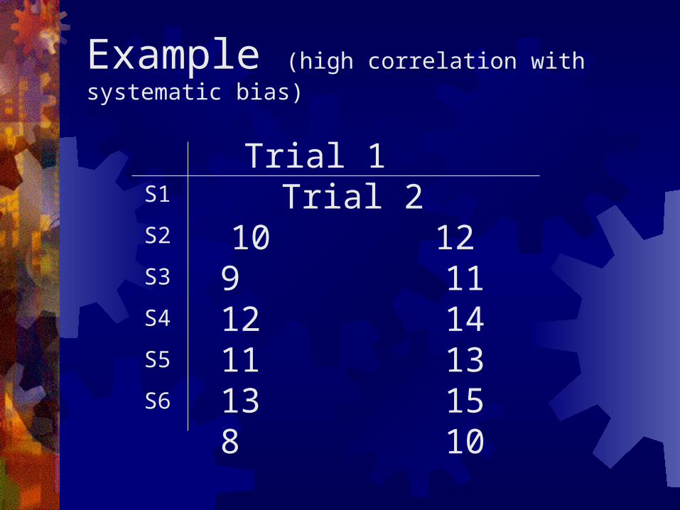
Example (high correlation with systematic bias)

Trial 1 Trial 210 129 1112 1411 1313 158 10

S1

S2

S3

S4

S5

S6

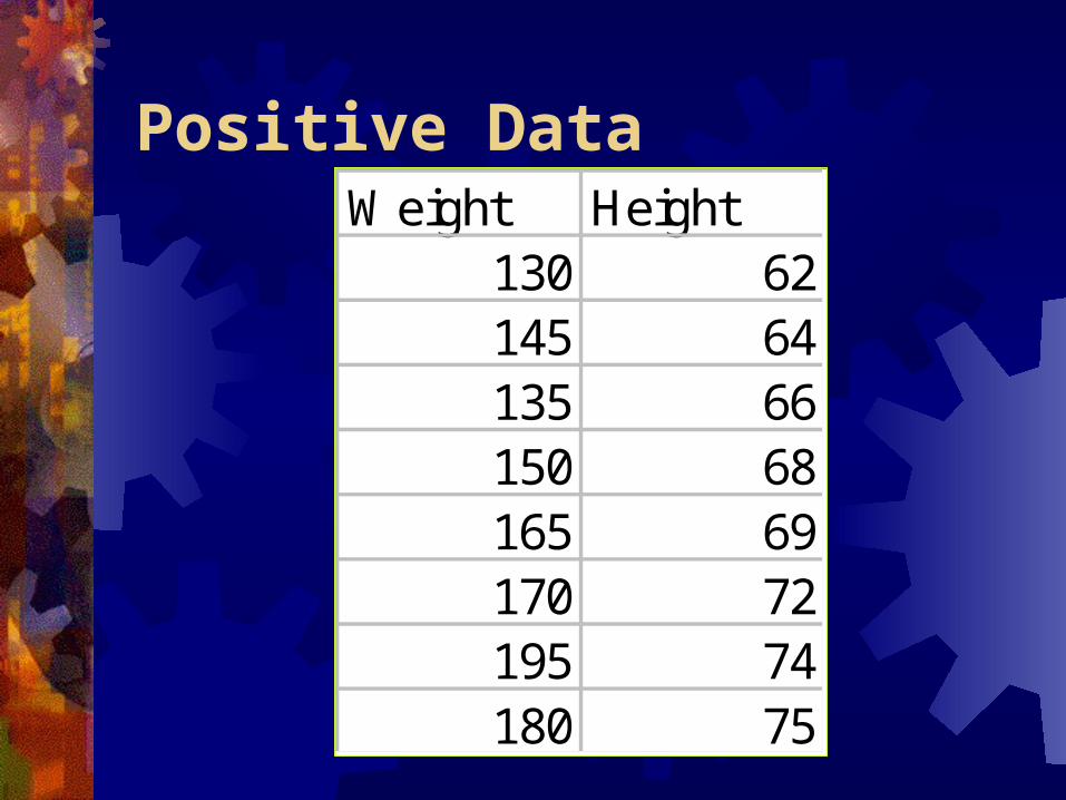
Positive DataWeight Height

130 62145 64135 66150 68165 69170 72195 74180 75

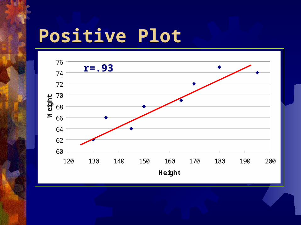
Positive Plot

60

62

64

66

68

70

72

74

76

120 130 140 150 160 170 180 190 200

Height

Wei

gh

t

r=.93

Negative DataWeight Sit-ups

180 62195 64170 66165 68150 69135 72145 74130 75

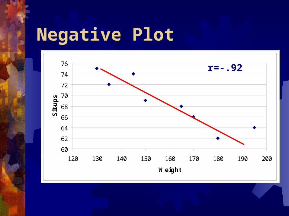
Negative Plot

60

62

64

66

68

70

72

74

76

120 130 140 150 160 170 180 190 200

Weight

Sit

-up

s

r=-.92

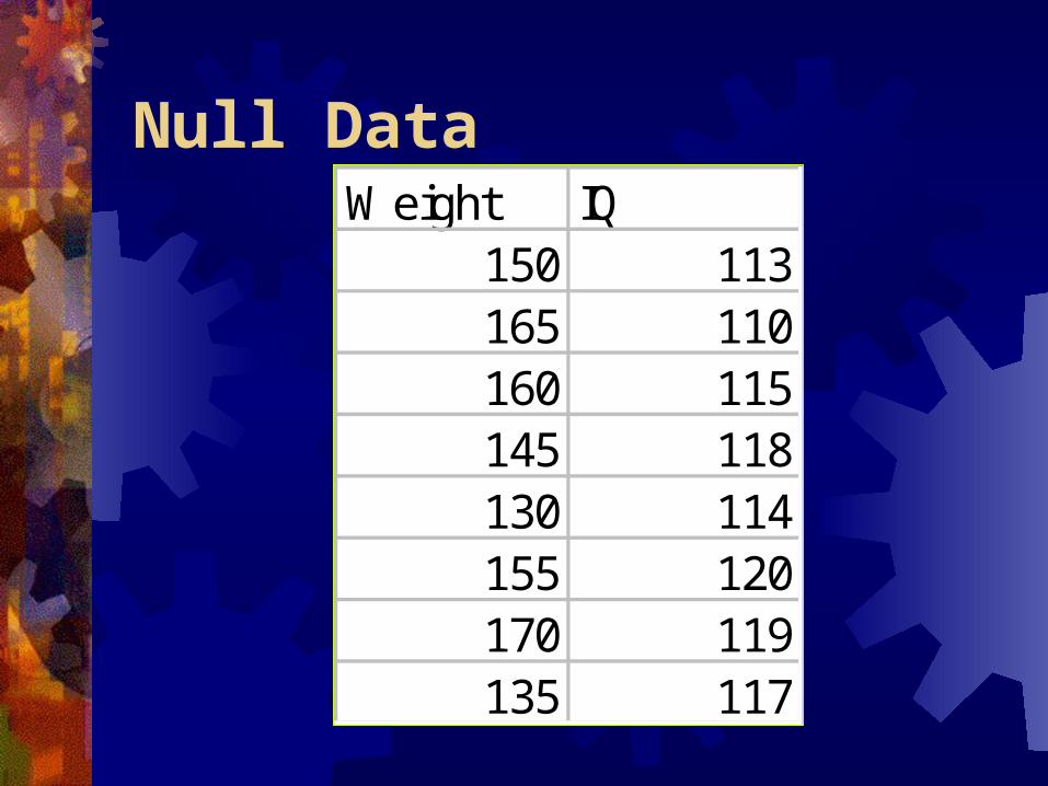
Null DataWeight IQ

150 113165 110160 115145 118130 114155 120170 119135 117

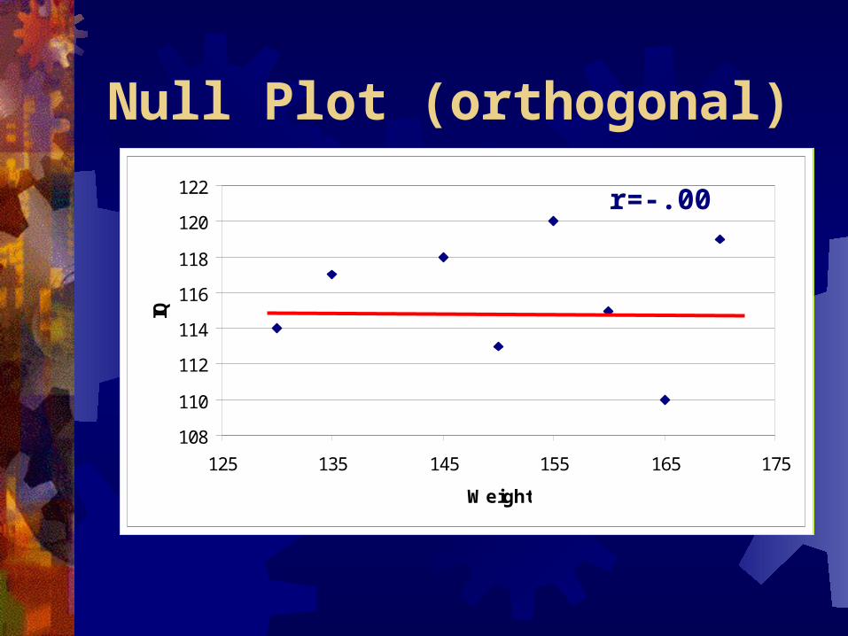
Null Plot (orthogonal)

r=.34

108

110

112

114

116

118

120

122

125 135 145 155 165 175

Weight

IQ

r=-.00

Pearson (Interclass Correlation)

• Ignores the systematic bias

• Has agreement (rank) but not correspondence (raw score)

• The order and the SD of the scores remain the same

• The mean may be different between the two tests• The r can still be high (i.e. close to 1.0)

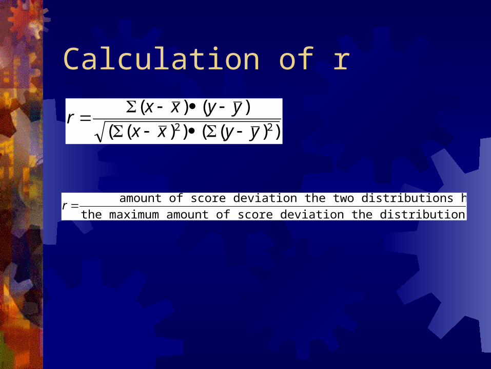
Calculation of r

rx x y y

x x y y

( ) ( )

( ( ) ) ( ( ) )2 2

r amount of score deviation the two distributions have in common

the maximum amount of score deviation the distributions could have in common

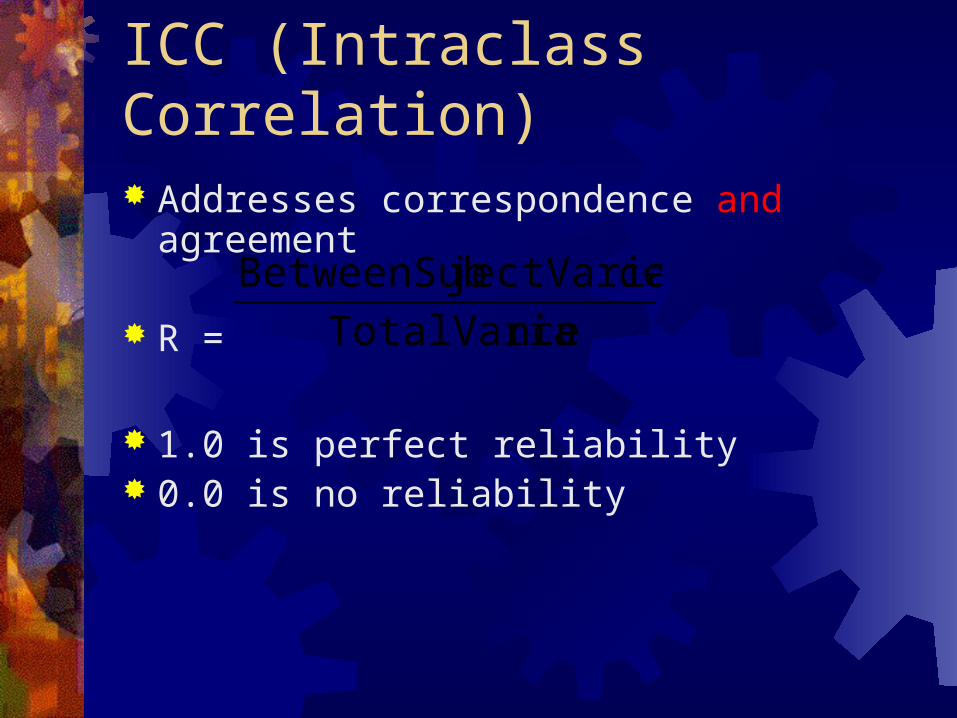
ICC (Intraclass Correlation) Addresses correspondence and agreement

R =

1.0 is perfect reliability 0.0 is no reliability

nceTotalVaria

cejectVarianBetweenSub

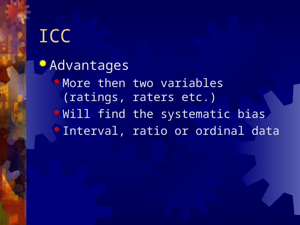
ICCAdvantages

More then two variables (ratings, raters etc.)

Will find the systematic bias Interval, ratio or ordinal data

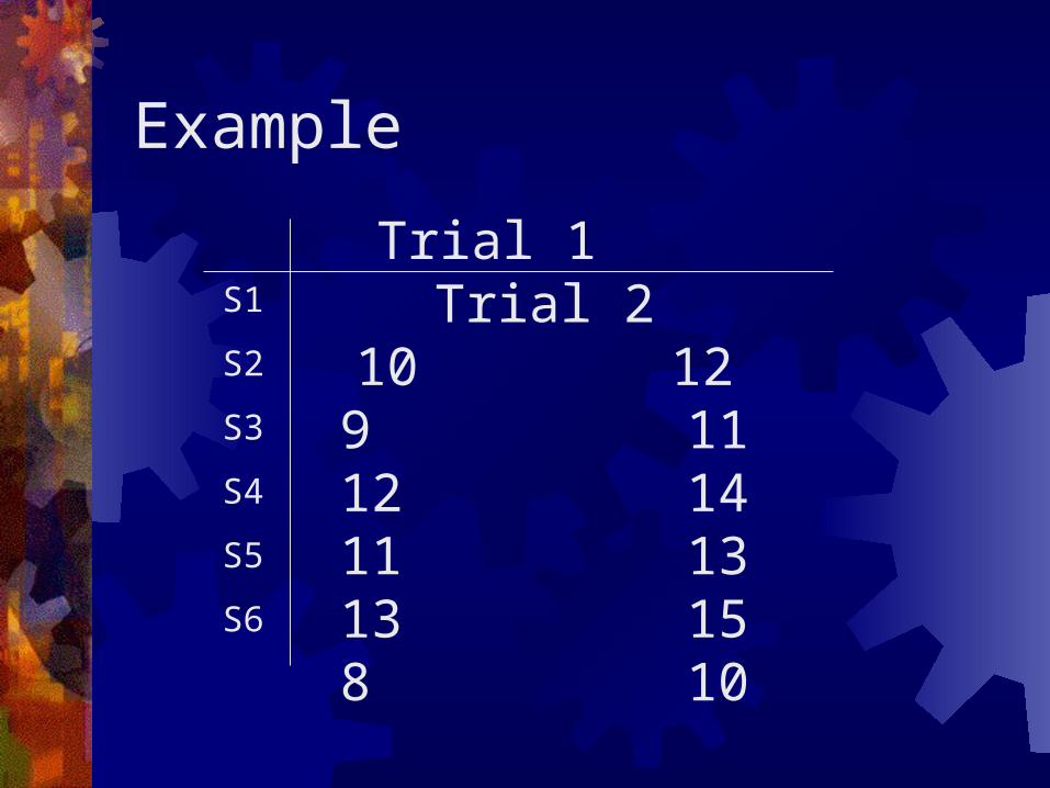
Example

Trial 1 Trial 210 129 1112 1411 1313 158 10

S1

S2

S3

S4

S5

S6

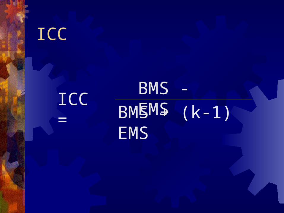
ICC

ICC =BMS - EMS

BMS + (k-1) EMS

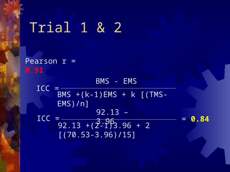
Trial 1 & 2

BMS - EMS

BMS +(k-1)EMS + k [(TMS-EMS)/n]ICC =

92.13 – 3.96

92.13 +(2-1)3.96 + 2 [(70.53-3.96)/15]ICC = = 0.84

Pearson r = 0.91

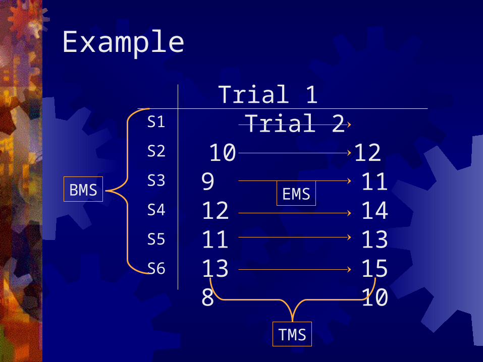
Example

Trial 1 Trial 210 129 1112 1411 1313 158 10

S1

S2

S3

S4

S5

S6

BMS

TMS

EMS

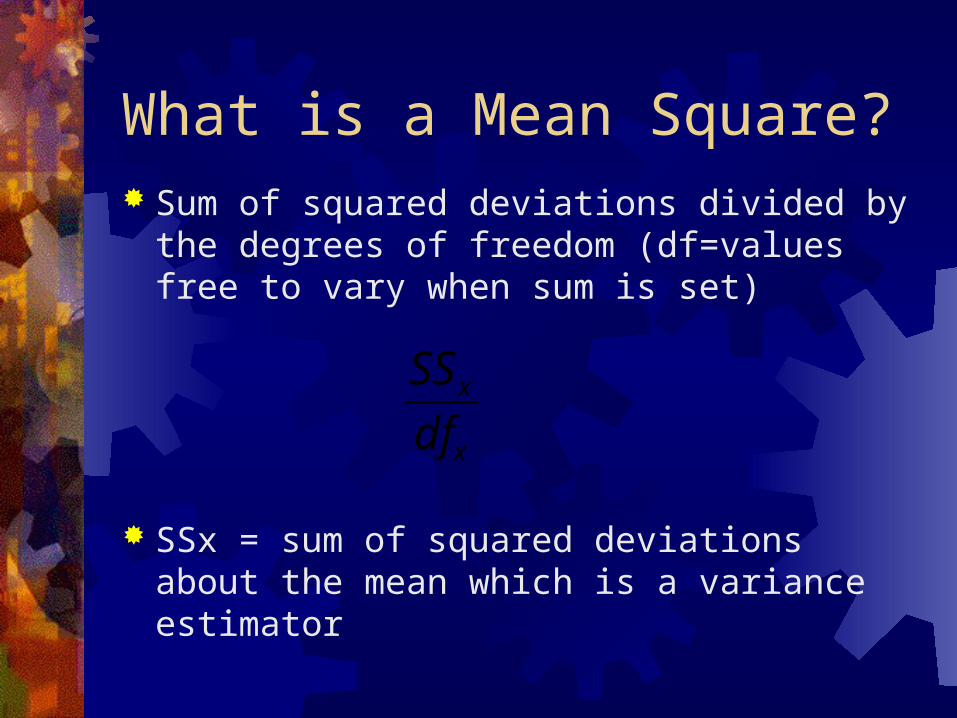
What is a Mean Square? Sum of squared deviations divided by the

degrees of freedom (df=values free to vary when sum is set)

SSx = sum of squared deviations about the mean which is a variance estimator

x

x

df

SS

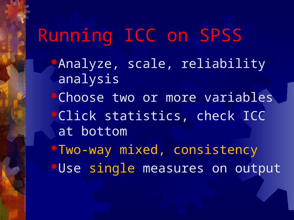
Running ICC on SPSS

Analyze, scale, reliability analysisChoose two or more variablesClick statistics, check ICC at

bottomTwo-way mixed, consistency Use single measures on output

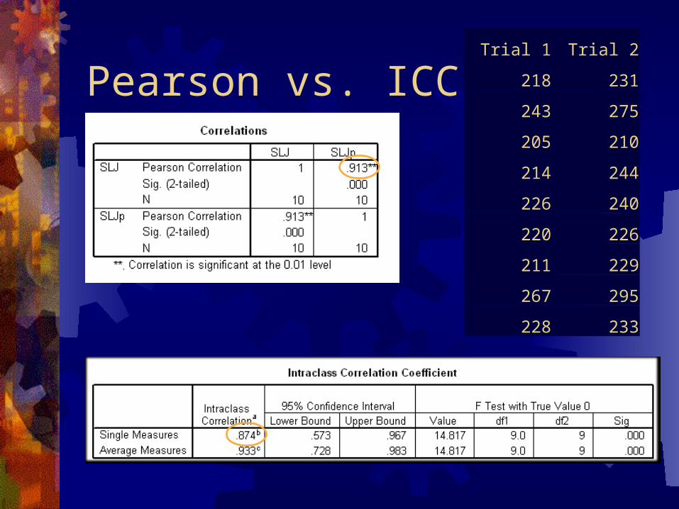
Pearson vs. ICCTrial 1 Trial 2

218 231

243 275

205 210

214 244

226 240

220 226

211 229

267 295

228 233

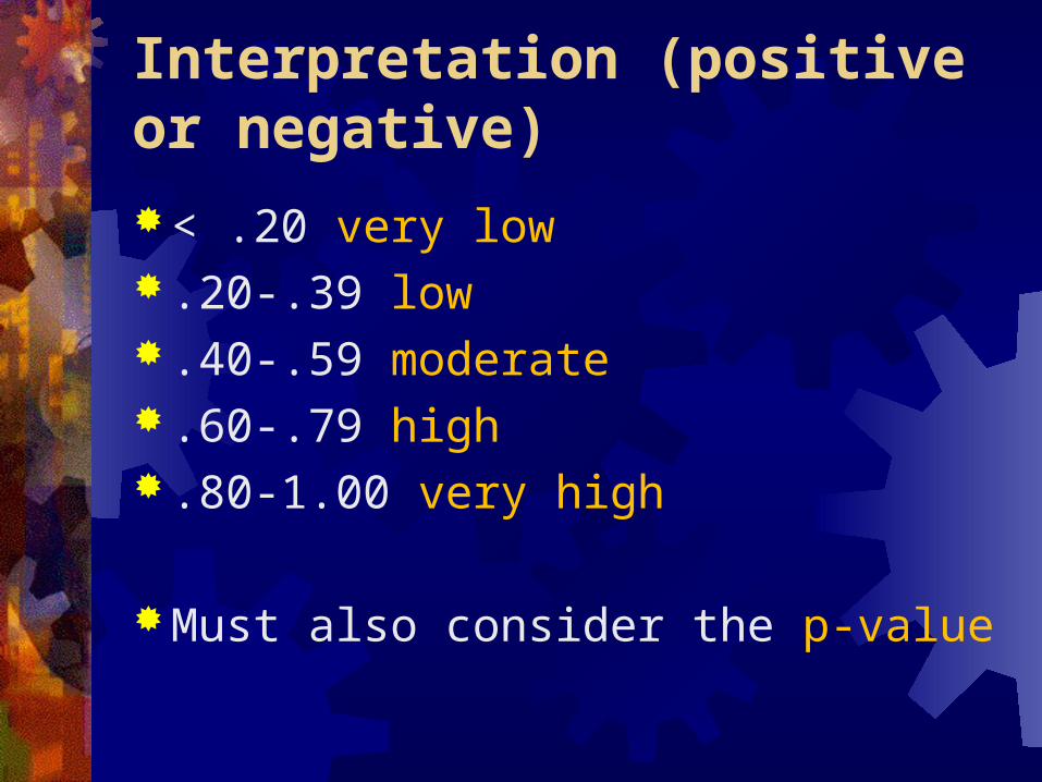
Interpretation (positive or negative)

< .20 very low .20-.39 low .40-.59 moderate .60-.79 high .80-1.00 very high

Must also consider the p-value

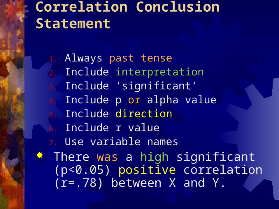
Correlation Conclusion Statement

1. Always past tense2. Include interpretation3. Include ‘significant’4. Include p or alpha value5. Include direction6. Include r value7. Use variable names

There was a high significant (p<0.05) positive correlation (r=.78) between X and Y.

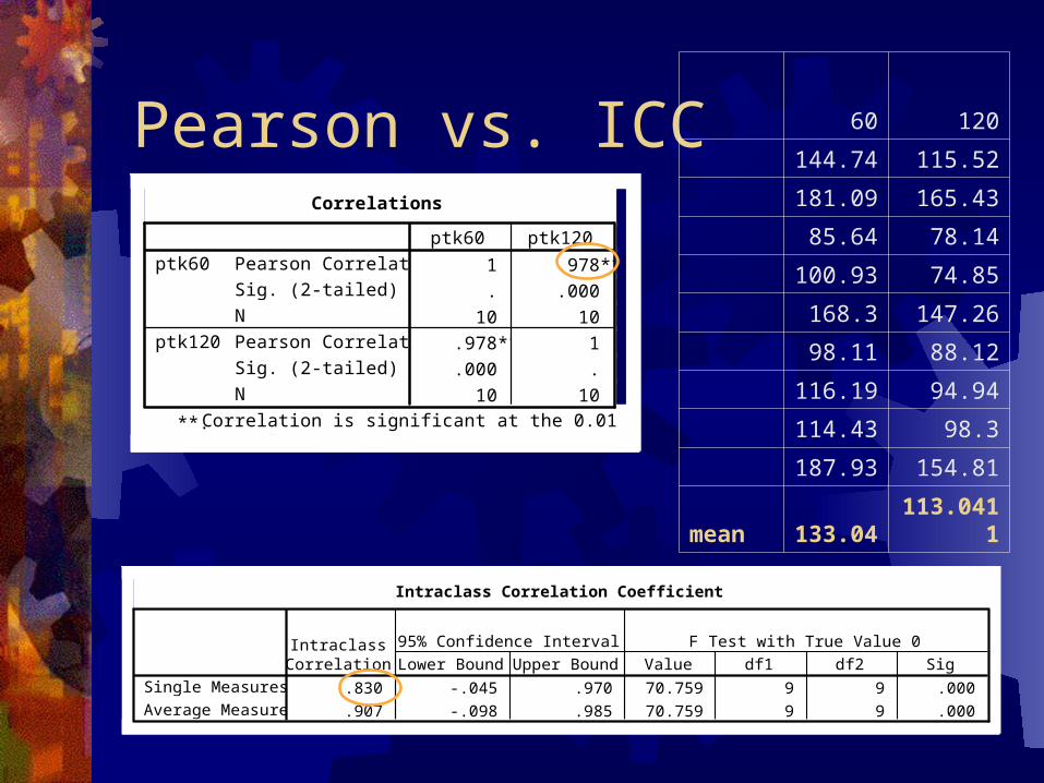
Pearson vs. ICC 60 120

144.74 115.52

181.09 165.43

85.64 78.14

100.93 74.85

168.3 147.26

98.11 88.12

116.19 94.94

114.43 98.3

187.93 154.81

mean 133.04 113.0411

Correlations

1 .978**

. .000

10 10

.978** 1

.000 .

10 10

Pearson Correlation

Sig. (2-tailed)

N

Pearson Correlation

Sig. (2-tailed)

N

ptk60

ptk120

ptk60 ptk120

Correlation is significant at the 0.01 level(2-tailed).

**.

Intraclass Correlation Coefficient

.830 -.045 .970 70.759 9 9 .000

.907 -.098 .985 70.759 9 9 .000

Single Measures

Average Measures

IntraclassCorrelation Lower Bound Upper Bound

95% Confidence Interval

Value df1 df2 Sig

F Test with True Value 0

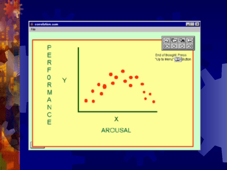
CurvilinearScores curve around line of best fit.Also called a trend analysis.More complex statistics.

Coefficient of DeterminationRepresents the common variance

between scores.Square of the r value.% explained.How much one variable affects the

other

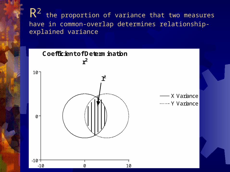
R2 the proportion of variance that two measures have in

common-overlap determines relationship-explained variance

Coefficient of Determinationr2

-10 0 10-10

0

10

X VarianceY Variance

r2

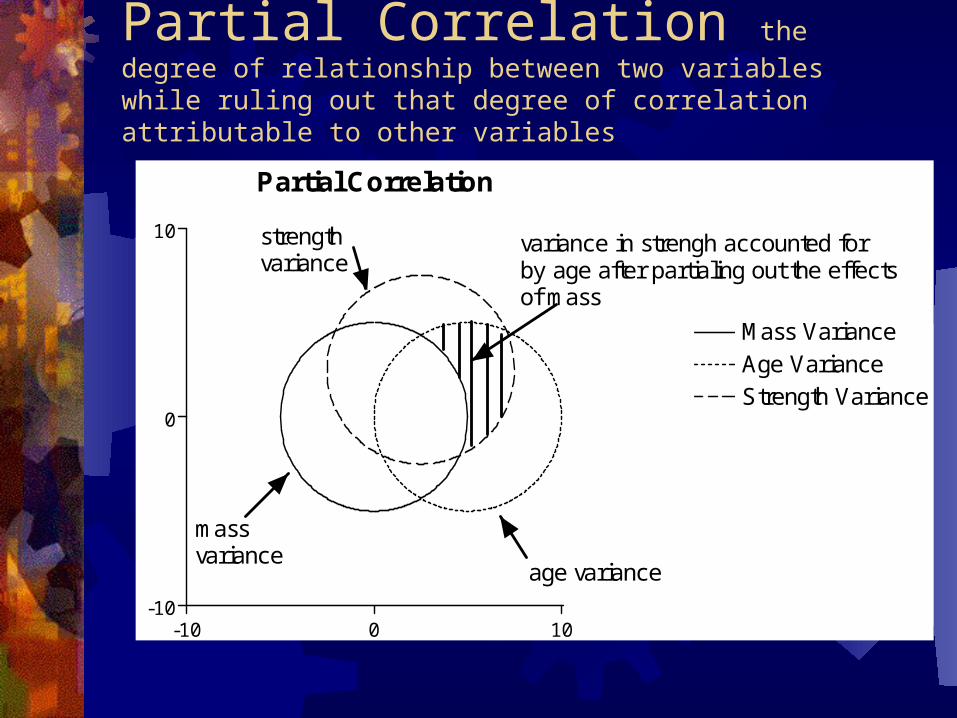
Partial Correlation the degree of relationship

between two variables while ruling out that degree of correlation attributable to other variables

Partial Correlation

-10 0 10-10

0

10

Mass VarianceAge VarianceStrength Variance

strengthvariance

massvariance

age variance

variance in strengh accounted forby age after partialing out the effectsof mass

Simple Linear Regression

Predict one variable from one another If measurement on one variable is difficult

or missingPrediction is not perfect but contains errorHigh reliability if error is low and R is high

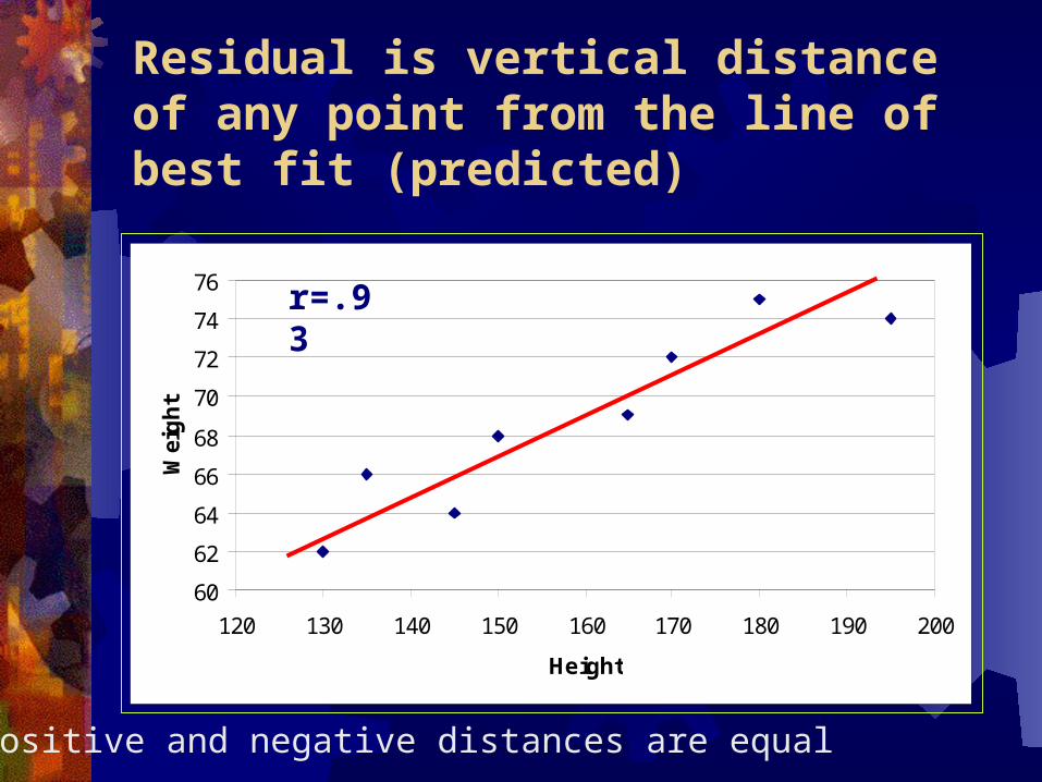
Residual is vertical distance of any point from the line of best fit (predicted)

60

62

64

66

68

70

72

74

76

120 130 140 150 160 170 180 190 200

Height

Wei

gh

t

r=.93

Positive and negative distances are equal

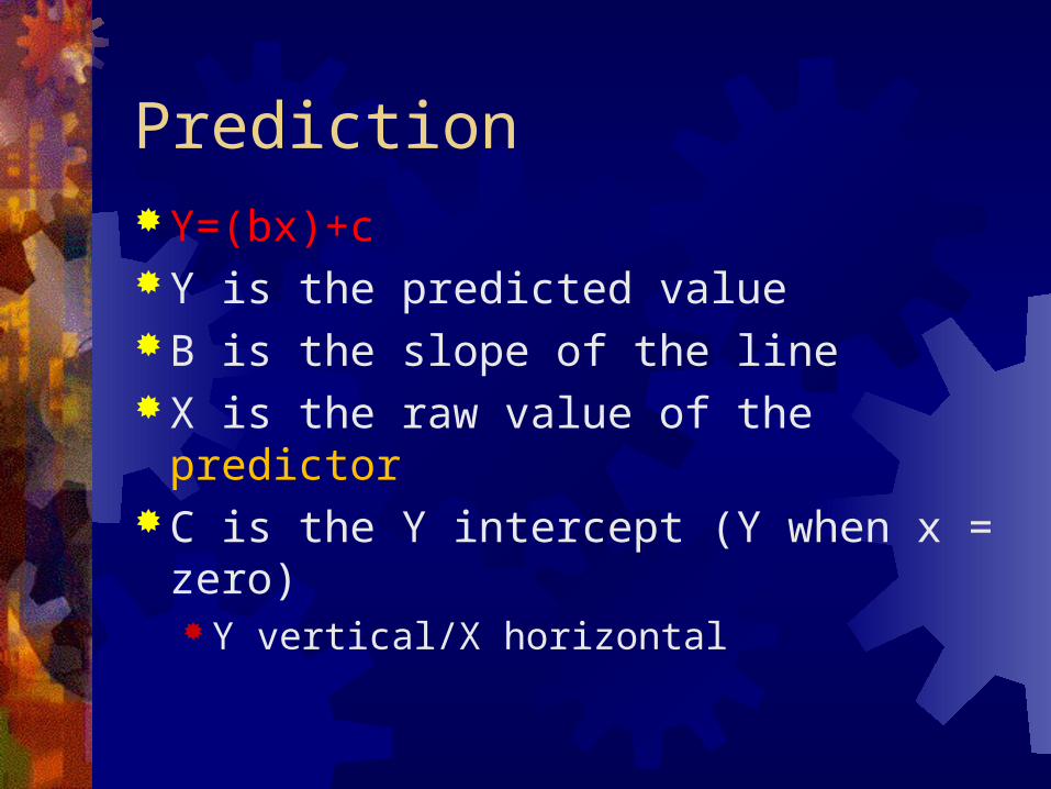
PredictionY=(bx)+cY is the predicted valueB is the slope of the lineX is the raw value of the predictorC is the Y intercept (Y when x = zero)

Y vertical/X horizontal

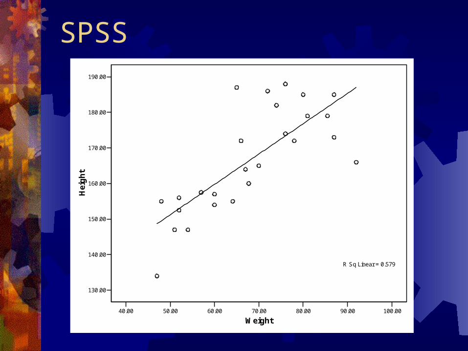
SPSS

40.00 50.00 60.00 70.00 80.00 90.00 100.00

Weight

130.00

140.00

150.00

160.00

170.00

180.00

190.00H

eig

ht

R Sq Linear = 0.579

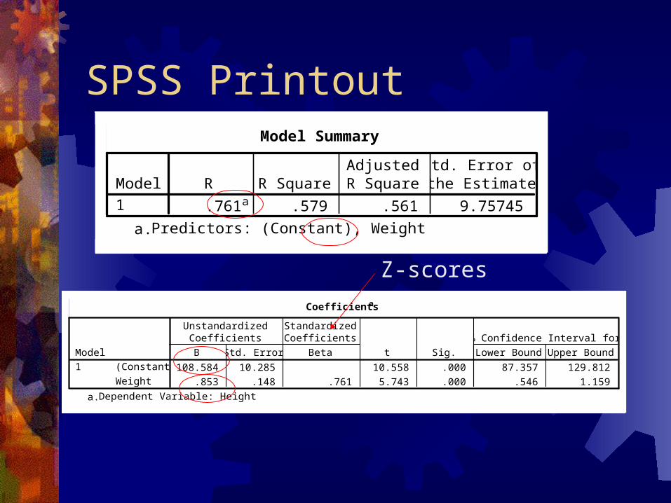
SPSS PrintoutModel Summary

.761a .579 .561 9.75745Model1

R R SquareAdjustedR Square

Std. Error ofthe Estimate

Predictors: (Constant), Weighta.

Coefficientsa

108.584 10.285 10.558 .000 87.357 129.812

.853 .148 .761 5.743 .000 .546 1.159

(Constant)

Weight

Model1

B Std. Error

UnstandardizedCoefficients

Beta

StandardizedCoefficients

t Sig. Lower Bound Upper Bound

95% Confidence Interval for B

Dependent Variable: Heighta.

Z-scores

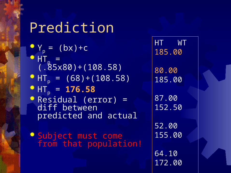
Prediction Yp = (bx)+c HTp = (.85x80)+(108.58) HTp = (68)+(108.58) HTp = 176.58 Residual (error) = diff

between predicted and actual

Subject must come from that population!

HT WT185.00 80.00185.00 87.00152.50 52.00155.00 64.10172.00 66.00179.00 81.00160.00 67.72174.00 76.00154.00 60.00165.00 70.00

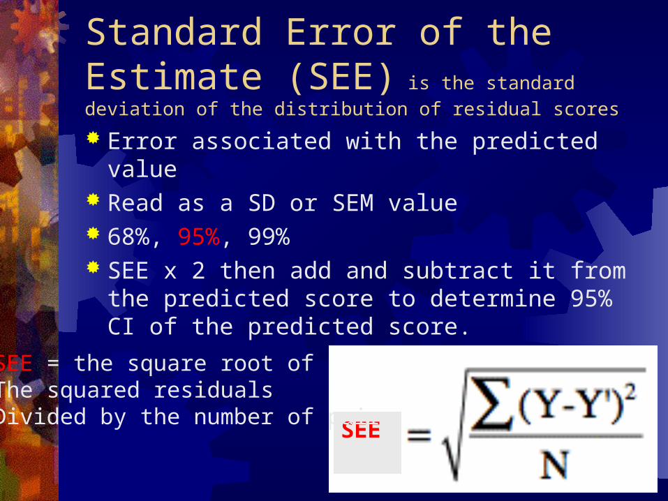
Standard Error of the Estimate (SEE) is the standard deviation of the distribution of residual

scores

Error associated with the predicted value Read as a SD or SEM value 68%, 95%, 99% SEE x 2 then add and subtract it from the

predicted score to determine 95% CI of the predicted score.

SEE

SEE = the square root of The squared residuals Divided by the number of pairs

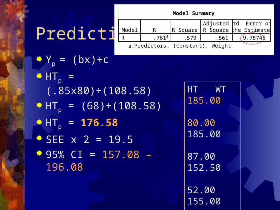
Prediction Yp = (bx)+c

HTp = (.85x80)+(108.58)

HTp = (68)+(108.58)

HTp = 176.58

SEE x 2 = 19.5 95% CI = 157.08 – 196.08

HT WT185.00 80.00185.00 87.00152.50 52.00155.00 64.10172.00 66.00179.00 81.00160.00 67.72174.00 76.00154.00 60.00165.00 70.00

Model Summary

.761a .579 .561 9.75745Model1

R R SquareAdjustedR Square

Std. Error ofthe Estimate

Predictors: (Constant), Weighta.

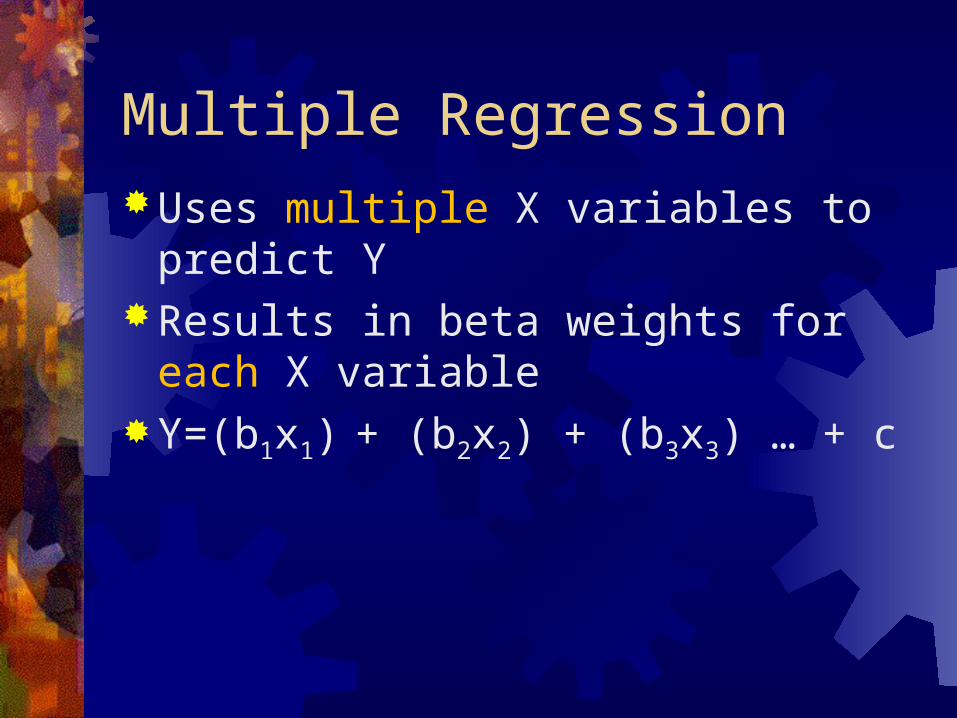
Multiple RegressionUses multiple X variables to predict YResults in beta weights for each X

variableY=(b1x1) + (b2x2) + (b3x3) … + c

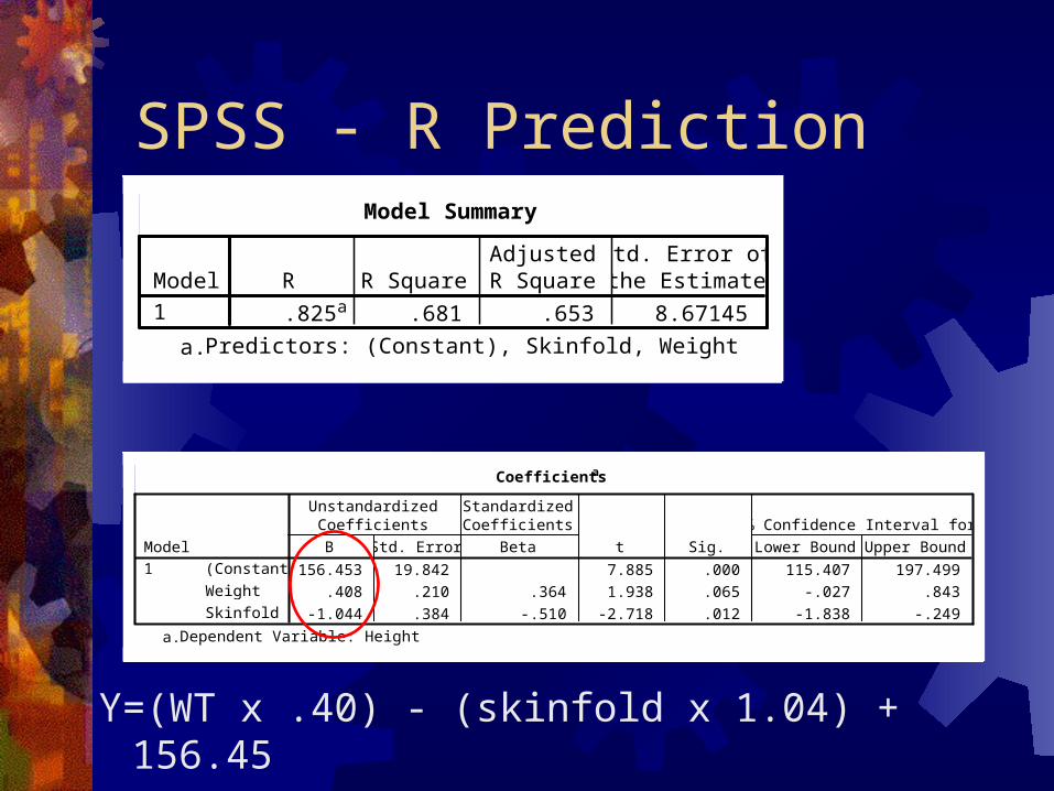
SPSS - R PredictionModel Summary

.825a .681 .653 8.67145Model1

R R SquareAdjustedR Square

Std. Error ofthe Estimate

Predictors: (Constant), Skinfold, Weighta.

Coefficientsa

156.453 19.842 7.885 .000 115.407 197.499

.408 .210 .364 1.938 .065 -.027 .843

-1.044 .384 -.510 -2.718 .012 -1.838 -.249

(Constant)

Weight

Skinfold

Model1

B Std. Error

UnstandardizedCoefficients

Beta

StandardizedCoefficients

t Sig. Lower Bound Upper Bound

95% Confidence Interval for B

Dependent Variable: Heighta.

Y=(WT x .40) - (skinfold x 1.04) + 156.45

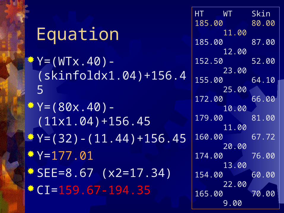
EquationY=(WTx.40)-

(skinfoldx1.04)+156.45Y=(80x.40)-

(11x1.04)+156.45Y=(32)-(11.44)+156.45Y=177.01SEE=8.67 (x2=17.34)CI=159.67-194.35

HT WT Skin185.00 80.00 11.00185.00 87.00 12.00152.50 52.00 23.00155.00 64.10 25.00172.00 66.00 10.00179.00 81.00 11.00160.00 67.72 20.00174.00 76.00 13.00154.00 60.00 22.00165.00 70.00 9.00

Next ClassChapter 8 & 13 t-tests and chi-square.

Homework1. Make a scatterplot with trendline and r and

r2 of two ratio variables.2. Run Pearson r on four different variables

and hand draw a scatterplot for two.3. Run ICC between VJ1 and VJ2.4. Run linear regression on standing long jump

and predict stair up time. Work out the equation and CI for subject #2.

5. Run multiple regression on subject #2 and add vjump running, circumference and weight to predictors. Also out the equation and CI.