Finite  Element  Method  I  

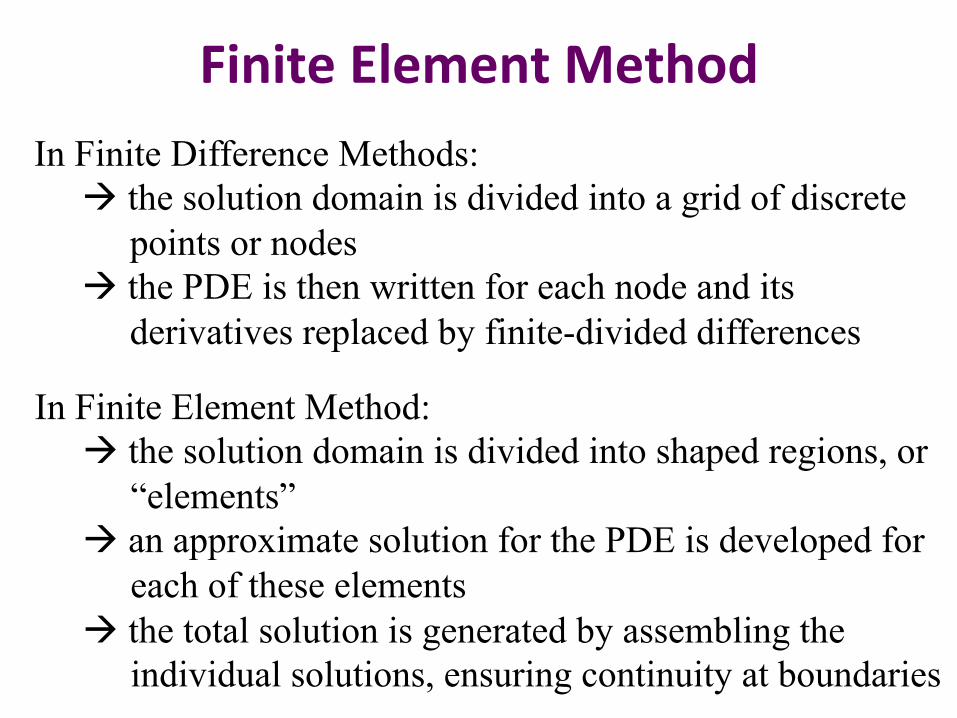
Finite  Element  Method  In Finite Difference Methods:

à the solution domain is divided into a grid of discrete points or nodes à the PDE is then written for each node and its

derivatives replaced by finite-divided differences

In Finite Element Method: à the solution domain is divided into shaped regions, or

“elements” à an approximate solution for the PDE is developed for

each of these elements à the total solution is generated by assembling the

individual solutions, ensuring continuity at boundaries

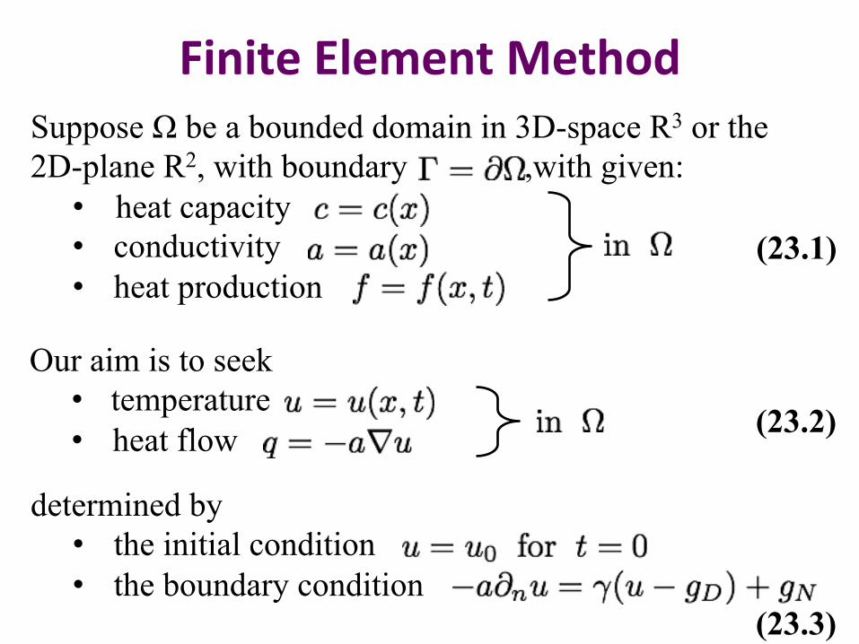
Finite  Element  Method  Suppose Ω be a bounded domain in 3D-space R3 or the 2D-plane R2, with boundary ,with given: •  heat capacity •  conductivity •  heat production

Our aim is to seek •  temperature •  heat flow

determined by •  the initial condition •  the boundary condition

(23.1)

(23.2)

(23.3)

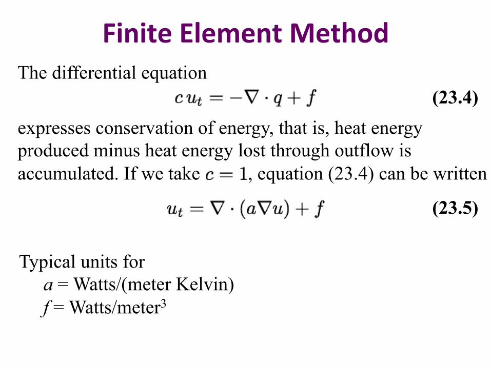
Finite  Element  Method  

expresses conservation of energy, that is, heat energy produced minus heat energy lost through outflow is accumulated. If we take , equation (23.4) can be written

(23.4)

Typical units for a = Watts/(meter Kelvin) f = Watts/meter3

The differential equation

(23.5)

Finite  Element  Method  For time discretization of the problem, we introduce:

For space discretization of the problem, using finite elements, we introduce a triangulation of Ω:

x1   x2  

x3  x5  

x6  

x4  

x7  

1   2  3  

4  5  

6  

Finite  Element  Method  

Basis functions are particular continuous piecewise linear functions on the given triangulation, and characterized by

Then the approximate solution of is a piecewise linear which can be represented in terms of the basis functions and (unknown) node values with formula

(23.6)

(23.7)

Finite  Element  Method  

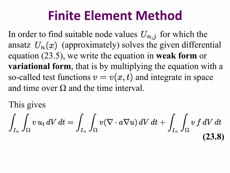
This gives

In order to find suitable node values for which the ansatz (approximately) solves the given differential equation (23.5), we write the equation in weak form or variational form, that is by multiplying the equation with a so-called test functions and integrate in space and time over Ω and the time interval.

(23.8)

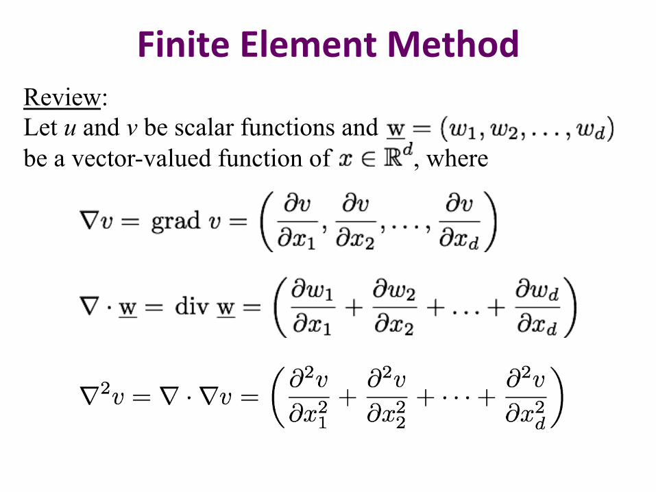
Finite  Element  Method  Review: Let u and v be scalar functions and be a vector-valued function of , where

Finite  Element  Method  

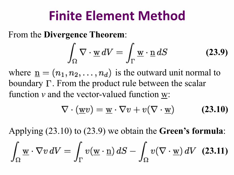
where is the outward unit normal to boundary . From the product rule between the scalar function v and the vector-valued function w:

From the Divergence Theorem:

(23.10)

(23.9)

Applying (23.10) to (23.9) we obtain the Green’s formula:

(23.11)

Finite  Element  Method  

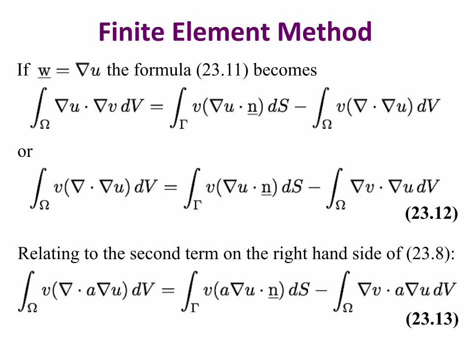
or

If the formula (23.11) becomes

(23.12)

Relating to the second term on the right hand side of (23.8):

(23.13)

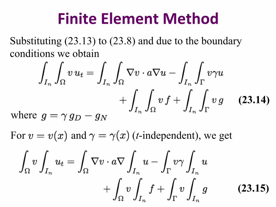
Finite  Element  Method  Substituting (23.13) to (23.8) and due to the boundary conditions we obtain

(23.15)

(23.14) where

For and (t-independent), we get

Finite  Element  Method  where

(23.16)

Thus, we seek

where which gives m equations for the m node values Un,j in the ansatz Un = Un(x).

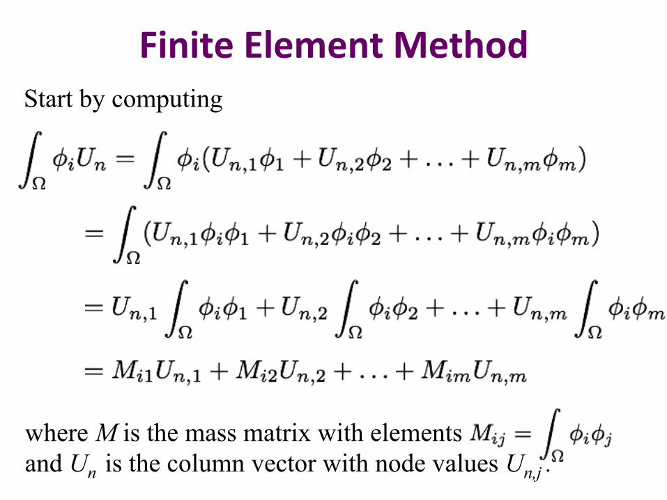
Finite  Element  Method  Start by computing

where M is the mass matrix with elements and Un is the column vector with node values Un,j .

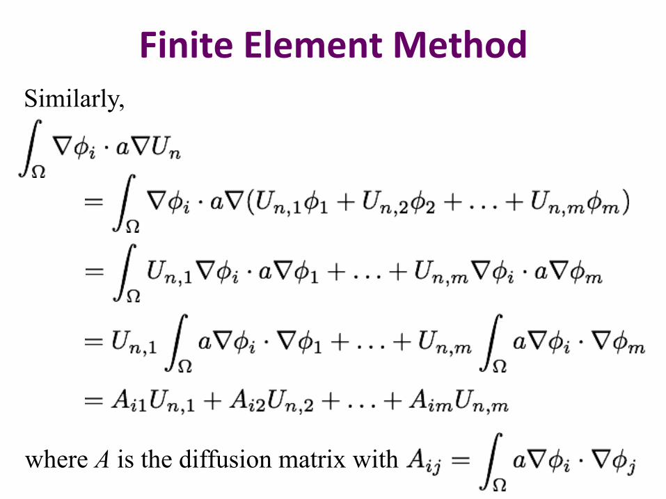
Finite  Element  Method  Similarly,

where A is the diffusion matrix with

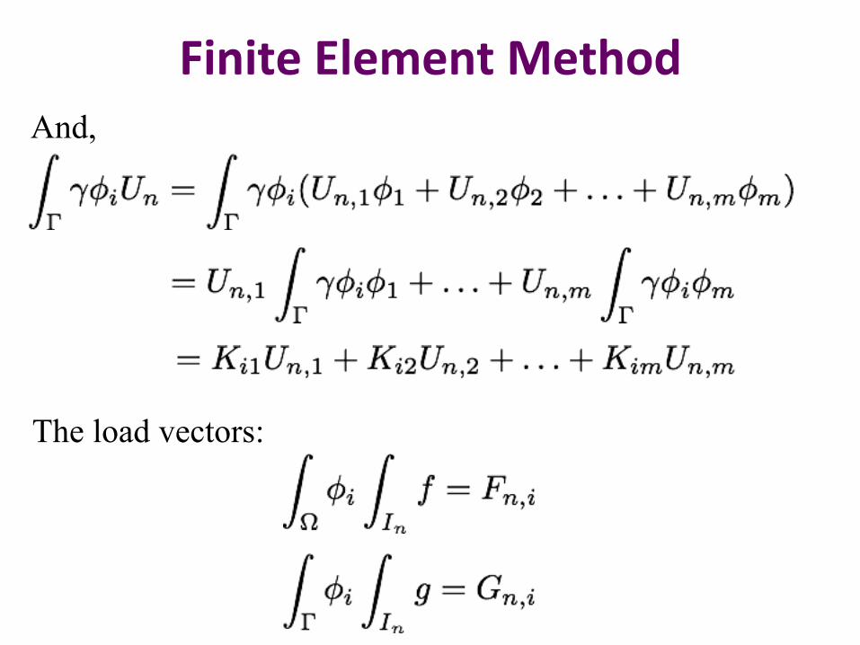
Finite  Element  Method  And,

The load vectors:

Finite  Element  Method  After perform approximation for all terms, we get a system of linearized approximations

(23.17) or

From which we can solve

where

MATLAB’s  pdetool  Toolbox  MATLAB has a GUI toolbox which is called pdetool that is used to solve linear PDEs based on finite element method. Basically the PDE toolbox can be used to solve the following problems:

1)  Elliptic PDEs 2)  Parabolic PDEs 3)  Hyperbolic PDEs 4)  Eigenmode PDE

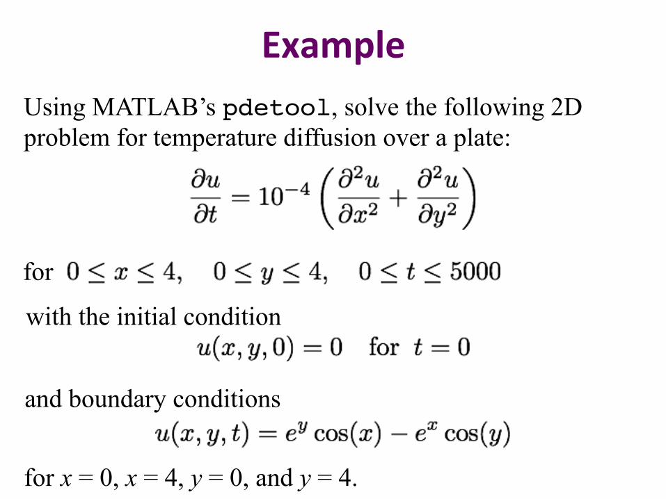
Example  Using MATLAB’s pdetool, solve the following 2D problem for temperature diffusion over a plate:

for

with the initial condition

and boundary conditions

for x = 0, x = 4, y = 0, and y = 4.

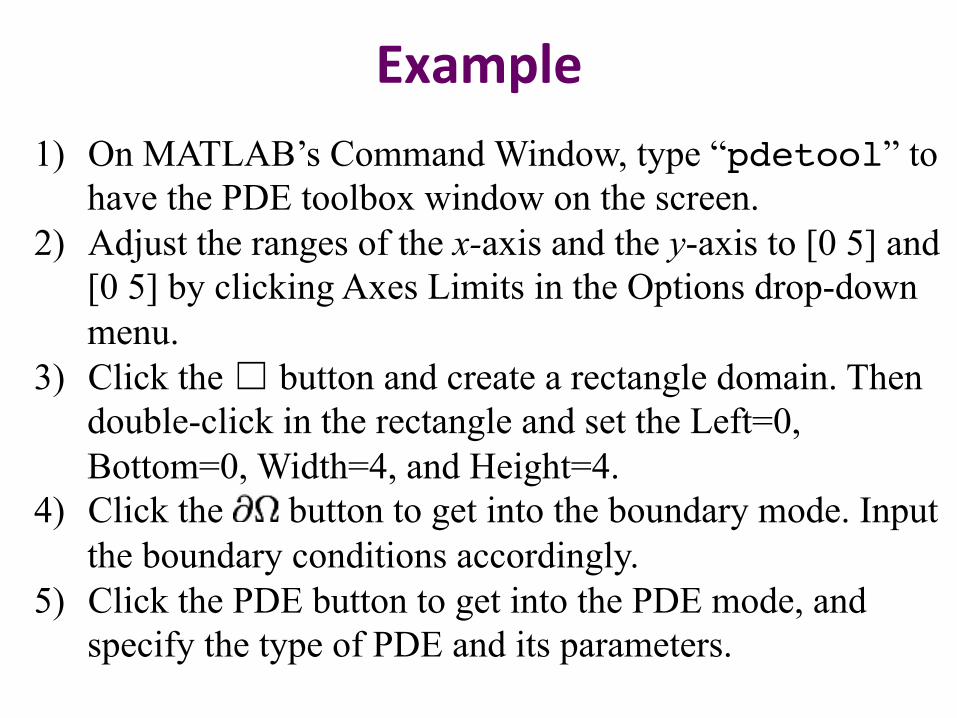
Example  1)  On MATLAB’s Command Window, type “pdetool” to

have the PDE toolbox window on the screen. 2)  Adjust the ranges of the x-axis and the y-axis to [0 5] and

[0 5] by clicking Axes Limits in the Options drop-down menu.

3)  Click the ☐ button and create a rectangle domain. Then double-click in the rectangle and set the Left=0, Bottom=0, Width=4, and Height=4.

4)  Click the button to get into the boundary mode. Input the boundary conditions accordingly.

5)  Click the PDE button to get into the PDE mode, and specify the type of PDE and its parameters.

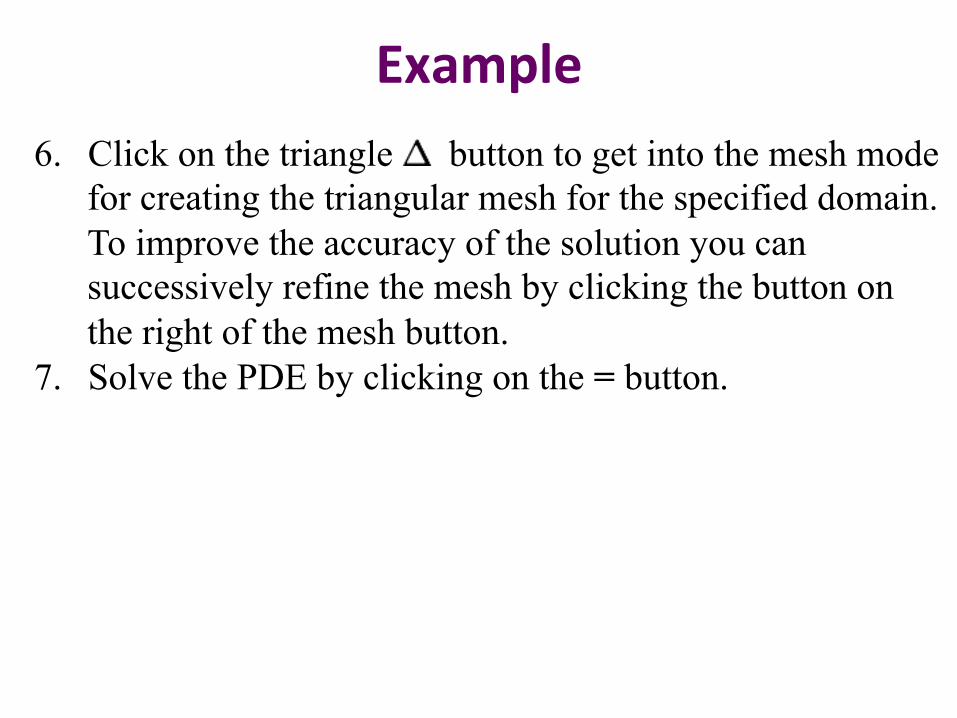
Example  6.  Click on the triangle button to get into the mesh mode

for creating the triangular mesh for the specified domain. To improve the accuracy of the solution you can successively refine the mesh by clicking the button on the right of the mesh button.

7.  Solve the PDE by clicking on the = button.

References  1)  Computational Differential Equations; K. Eriksson, D.

Estep, P. Hansbo, C. Johnson. 2)  Finite Element Methods Lecture Notes, K. Eriksson