the finite element method - tamu...
TRANSCRIPT
JN Reddy
The Finite Element Method
Read: Chs. 3 and 4
1D Problems Governed by Second-Order Equation
CONTENTS• Model differential equation • Finite element approximation • Finite element discretization• Development of weak form and
the definition of primary and secondary variables (duality)
• Essential and natural BCs• Linear and bilinear forms • Finite element model • Interpolation functions• Assembly of elements • Numerical examples
JN Reddy
When you are analyzing an engineering problem using a FEM program, you should know: (1) the mathematical model (governing
equations) that the program is solving, (2) the duality pairs for specifying the boundary
conditions, and (3) know the restrictions of the mathematical and
computational models.
Important Comments• Knowing is power. Your confidence in what you
do goes up.
• Mathematics is the language of an engineer.
• “Mathematics is the language with which God has written the universe.” −Galileo Galilei
JN Reddy
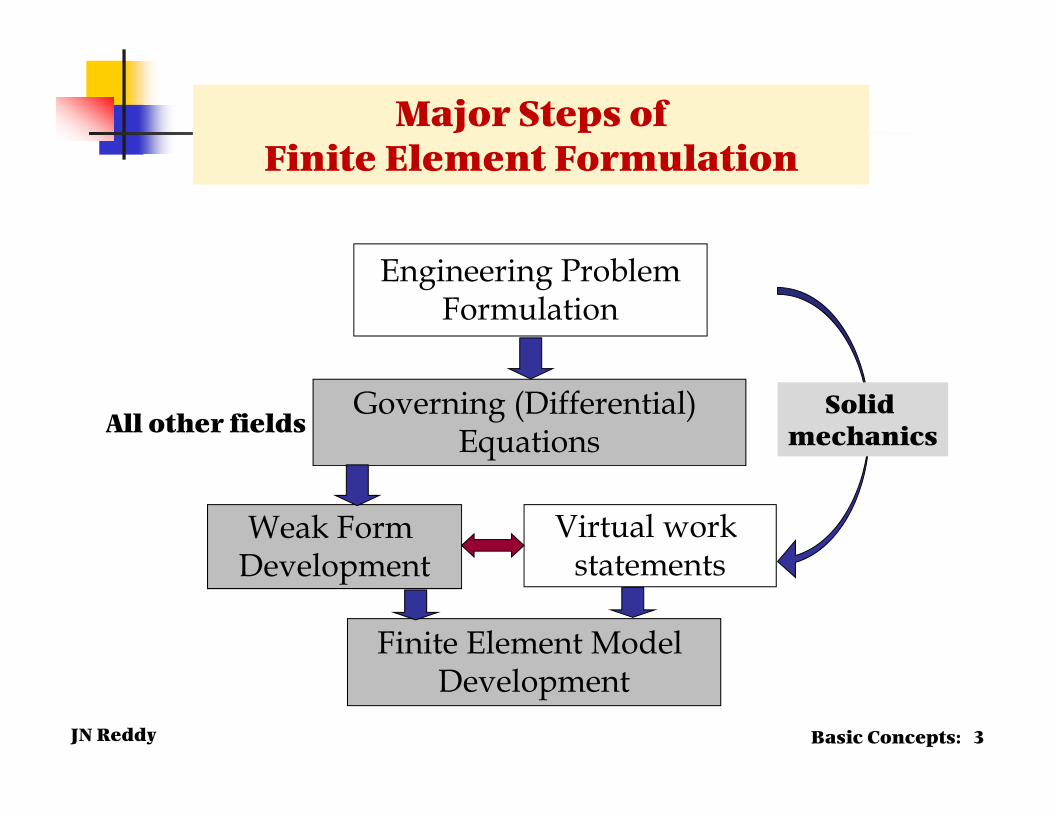
Major Steps of Finite Element Formulation
Finite Element Model Development
Governing (Differential) Equations
Engineering ProblemFormulation
Virtual work statements
Weak Form Development
Basic Concepts: 3
Solid mechanicsAll other fields
JN Reddy Basic Concepts: 4
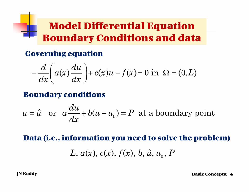
Model Differential Equation Boundary Conditions and data
0ˆ, ( ), ( ), ( ), , , ,L a x c x f x b u u P
Data (i.e., information you need to solve the problem)
0 0( ) ( ) ( ) in ( , )d dua x c x u f x Ldx dx
− + − = Ω =
Governing equation
0ˆ or ( ) at a boundary pointduu u a b u u Pdx
= + − =
Boundary conditions
JN Reddy
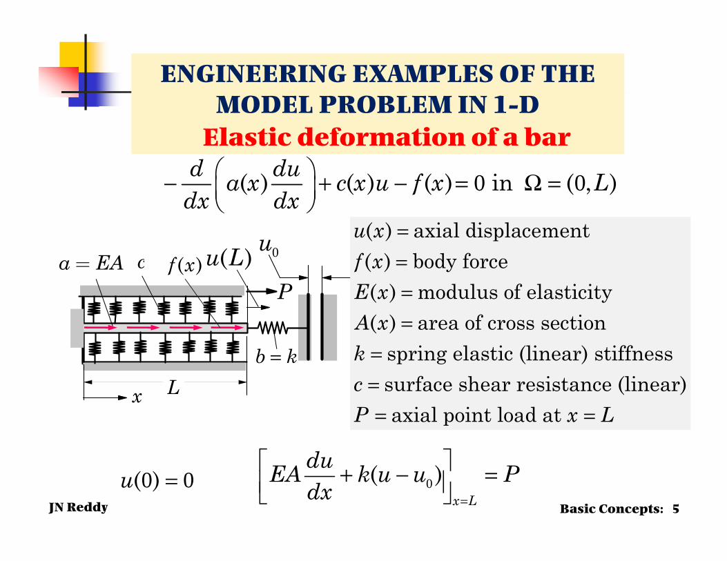
ENGINEERING EXAMPLES OF THE MODEL PROBLEM IN 1-D
Basic Concepts: 5
Elastic deformation of a bar
( )f xa EA=0u
P( )u L
b k=
x L
c
0 0( ) ( ) ( ) in ( , )d dua x c x u f x Ldx dx
− + − = Ω =
0 0( )u =
( ) axial displacement( ) body force( ) modulus of elasticity( ) area of cross section
spring elastic (linear) stiffnesssurface shear resistance (linear)axial point load at
u xf xE xA xkcP x L
====
=== =
0( )x L
duEA k u u Pdx =
+ − =
JN Reddy Introduction: 6
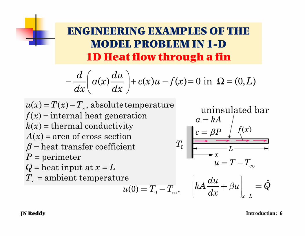
ENGINEERING EXAMPLES OF THE MODEL PROBLEM IN 1-D
1D Heat flow through a fin
0 0( ) ( ) ( ) in ( , )d dua x c x u f x Ldx dx
− + − = Ω =
( ) ( ) , absolutetemperature( ) internal heat generation( ) thermal conductivity( ) area of cross section
heat transfer coefficientperimeterheat input at ambient temperature
u x T x Tf xk xA x
PQ x LT
β
∞
∞
= −===
=== ==
uninsulated bara kAc Pβ== ( )f x
xL
u T T¥= -
0T
ˆx L
dukA u Qdx
b=
é ùê ú+ =ê úë û00( ) ,u T T¥= -
JN Reddy
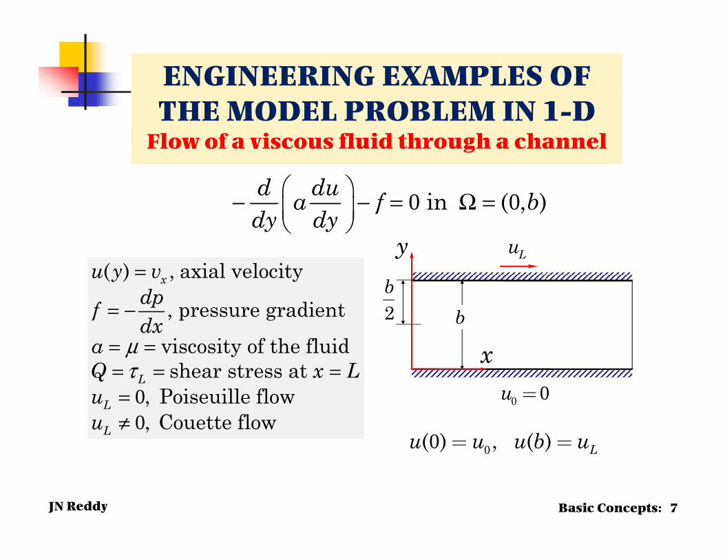
ENGINEERING EXAMPLES OF THE MODEL PROBLEM IN 1-D
Flow of a viscous fluid through a channel
Basic Concepts: 7
0 0in ( , )d dua f bdy dy
− − = Ω =
00
( ) , axial velocity
, pressure gradientviscosity of the fluidshear stress at
, Poiseuille flow, Couette flow
x
L
L
L
u y vdpfdx
aQ x Luu
μτ
=
= −
= == = ==≠
00( ) , ( ) Lu u u b u= =
Luy
b
x2b
0 0u =
JN Reddy
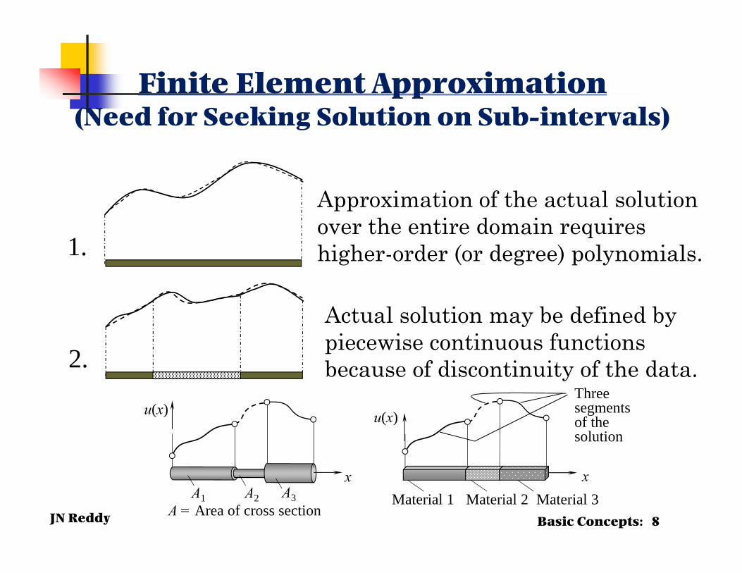
Finite Element Approximation(Need for Seeking Solution on Sub-intervals)
Approximation of the actual solutionover the entire domain requires higher-order (or degree) polynomials.1.
Actual solution may be defined by piecewise continuous functions because of discontinuity of the data.2.
A1 A2 A3A = Area of cross section
x
u(x)
Material 1 Material 2 Material 3x
u(x)Three segments of the solution
Basic Concepts: 8
JN Reddy
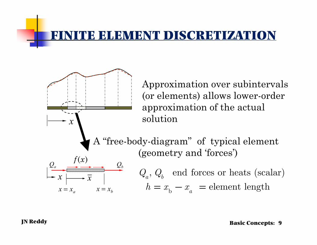
FINITE ELEMENT DISCRETIZATION
Approximation over subintervals (or elements) allows lower-order approximation of the actual solutionx
A “free-body-diagram” of typical element (geometry and ‘forces’)
b
, end forces or heats (scalar)
element lengtha b
a
Q Q
h x x= - =
Basic Concepts: 9
x xaQ bQ
axx = bxx =
( )f x

JN Reddy
{ }
0
0
( ) ( ) ( ) ( )
We seek to make ( ) zero in a weighted-residual sense:
( ) , is the weight function from a set of weight functions
( )
b
a
hh
x
i ixi
hi
dud a x c x u f x R xdx dx
R x
w R x dx ww
dudw a xdx dx
é ùæ ö÷çê ú- + - = ¹÷ç ÷çê úè øë û
=
æ öç= - ççè
ò
( ) ( )b
a
x
hxc x u f x dx
é ù÷ê ú+ -÷÷ê úøë ûò
Approximate Solution and Residual of the Approximation
Approximate solution: ( ) ( )hu x u x»
Basic Concepts: 10

JN Reddy
Product rule of differentiation (an identity) and integration-by-parts
( ) ( ) ( )
( ) ( ) ( )
h i h hi i
h h i hi i
du dw du dud dw a x a x w a xdx dx dx dx dx dx
du du dw dud dw a x w a x a xdx dx dx dx dx dx
æ ö æ ö÷ ÷ç ç= +÷ ÷ç ç÷ ÷ç çè ø è ø
æ ö æ ö÷ ÷ç ç- =- +÷ ÷ç ç÷ ÷ç çè ø è ø
Trading of Differentiation between the weight function and the variable
( ) ( ) ( )
( ) ( )
b b
a a
bb
aa
x xh h i h
i ix x
xx
i h hix
x
du du dw dud dw a x dx w a x a x dxdx dx dx dx dx dx
dw du dua x dx w a xdx dx dx
é ùæ ö æ ö÷ ÷ç çê ú- = - +÷ ÷ç ç÷ ÷ç çê úè ø è øë û
æ ö÷ç= - ÷ç ÷çè ø
ò ò
ò
Basic Concepts: 11
JN Reddy
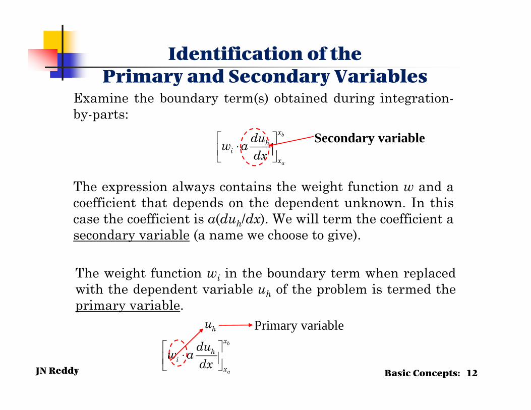
Examine the boundary term(s) obtained during integration-by-parts:
The expression always contains the weight function w and acoefficient that depends on the dependent unknown. In thiscase the coefficient is a(duh/dx). We will term the coefficient asecondary variable (a name we choose to give).
Identification of the Primary and Secondary Variables
b
a
xh
ix
duw adx
⋅
Secondary variable
The weight function wi in the boundary term when replacedwith the dependent variable uh of the problem is termed theprimary variable.
b
a
xh
ix
duw adx
⋅
hu Primary variable
Basic Concepts: 12
JN Reddy
0b
a
bb
aa
b
aa
xh
i hx
xx
i h hi h i ix
x
xi h h h
i h i i a i bxx
dudw a x c x u f x dxdx dx
dw du dua cw u w f dx w adx dx dx
dw du du dua cw u w f dx w x a w x adx dx dx dx
é ùæ ö÷çê ú= - + -÷ç ÷çê úè øë û
é ù é ùê ú ê ú= + - - ⋅ê ú ê úë û ë û
é ù æ ö æ ö÷ ÷ç çê ú= + - - ⋅ - - ⋅÷ ÷ç ç÷ç çê ú è ø è øë û
ò
ò
ò
( ) ( ) ( )
( ) ( )b
b
a
x
xi h
i h i i a i b bx
dw dua cw u w f dx w x Q w x Qdx dx
÷
é ùê ú= + - - - ⋅ê úë û
ò a( ) ( )
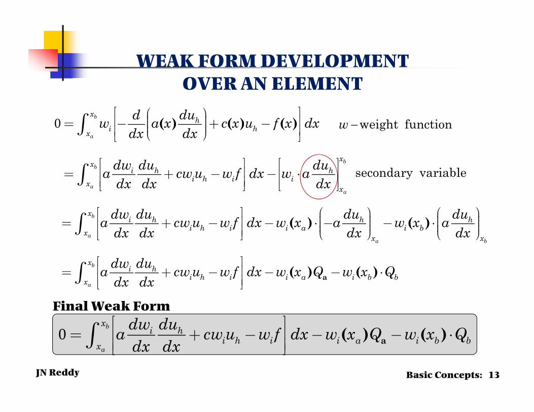
WEAK FORM DEVELOPMENT OVER AN ELEMENT
weight functionw −
secondary variable
Basic Concepts: 13
0b
a
xi h
i h i i a i b bx
dw dua cw u w f dx w x Q w x Qdx dx
é ùê ú= + - - - ⋅ê úë û
ò a( ) ( )
Final Weak Form
JN Reddy
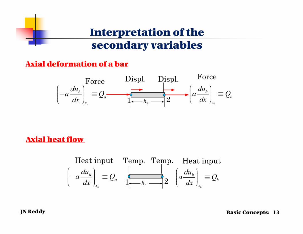
Interpretation of the secondary variables
Force
b
hb
x
dua Qdx
æ ö÷ç º÷ç ÷çè øa
ha
x
dua Qdx
æ ö÷ç- º÷ç ÷çè ø he 21
ForceDispl. Displ.
Axial deformation of a bar
Axial heat flow
Heat input
b
hb
x
dua Qdx
æ ö÷ç º÷ç ÷çè øa
ha
x
dua Qdx
æ ö÷ç- º÷ç ÷çè ø he 21
Heat inputTemp. Temp.
Basic Concepts: 13

JN Reddy
Primary variables and secondary variables alwaysappear in pairs. They are like `cause’ and `effect’ (i.e.,one is the result of the other). For example, when uh isthe temperature, a(duh/dx) is heat (and heat causestemperature). When uh is the displacement, a(duh/dx)is the force. This duality exists in every engineeringproblem.
Primary and Secondary Variables(Some Remarks)
Essential Boundary Conditions: Specifying a primaryvariable at a boundary point of the domain is called anessential (or Dirichlet) boundary condition.
Essential and Natural Boundary Conditions
Natural Boundary Conditions: Specifying a secondaryvariable at a boundary point of the domain is called anatural (or Neumann) boundary condition.
Basic Concepts: 15
JN Reddy
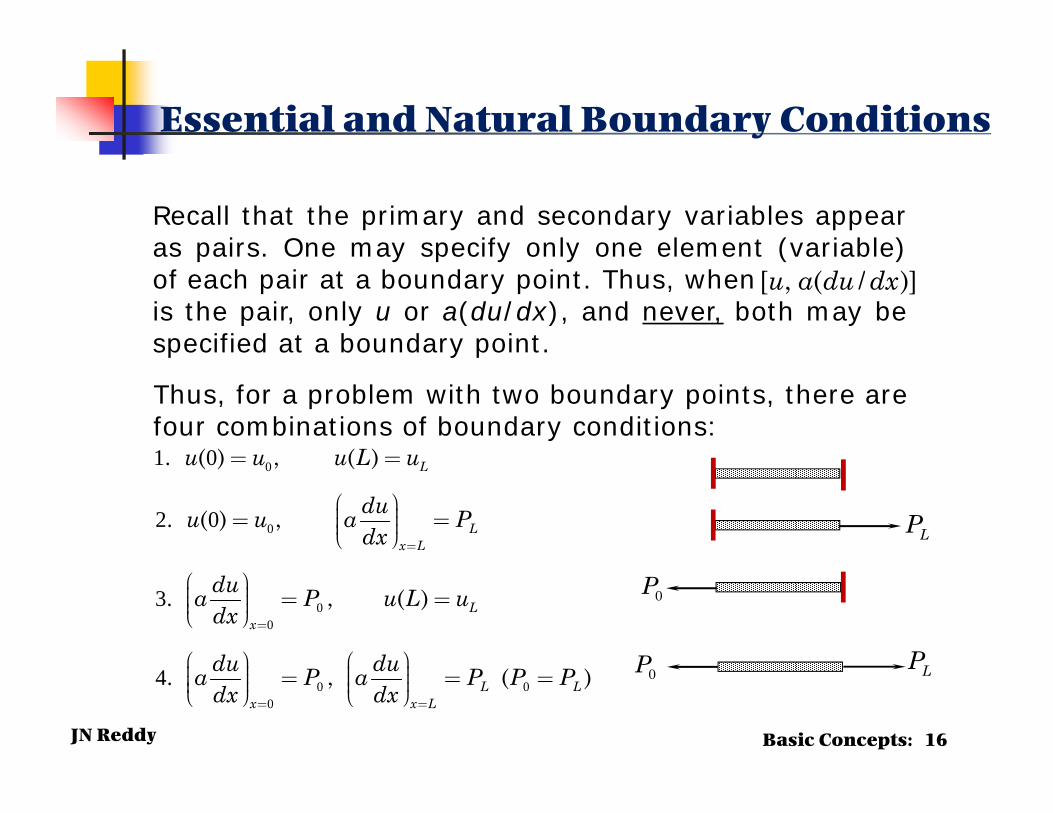
Recall that the primary and secondary variables appearas pairs. One may specify only one element (variable)of each pair at a boundary point. Thus, whenis the pair, only u or a(du/dx), and never, both may bespecified at a boundary point.
)]/(,[ dxduau
Essential and Natural Boundary Conditions
0
0
00
0 00
1 0
2 0
3
4
. ( ) , ( )
. ( ) ,
. , ( )
. , ( )
L
Lx L
Lx
L Lx x L
u u u L u
duu u a Pdx
dua P u L udx
du dua P a P P Pdx dx
=
=
= =
= =
æ ö÷ç= =÷ç ÷çè ø
æ ö÷ç = =÷ç ÷çè ø
æ ö æ ö÷ ÷ç ç= = =÷ ÷ç ç÷ ÷ç çè ø è ø
Thus, for a problem with two boundary points, there arefour combinations of boundary conditions:
0P LP
LP
0P
Basic Concepts: 16
JN Reddy
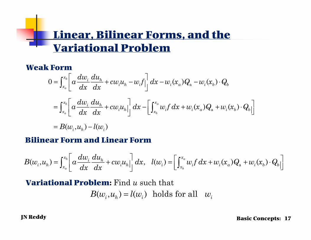
Linear, Bilinear Forms, and the Variational Problem
( , ) ( ) holds for all i h i iB w u l w w=
a( , ) , ( ) ( ) ( )b a
a b
x xi hi h i h i i i a i b bx x
dw duB w u a cw u dx l w w f dx w x Q w x Qdx dx
= + = + + ⋅
Bilinear Form and Linear Form
Weak Form
a
a
0 ( ) ( )
( ) ( )
( , ) ( )
b
a
b a
a b
x i hi h i i a i b bx
x xi hi h i i a i b bx x
i h i
dw dua cw u w f dx w x Q w x Qdx dx
dw dua cw u dx w f dx w x Q w x Qdx dx
B w u l w
= + − − − ⋅
= + − + + ⋅
= −
Variational Problem: Find u such that
Basic Concepts: 17
JN Reddy
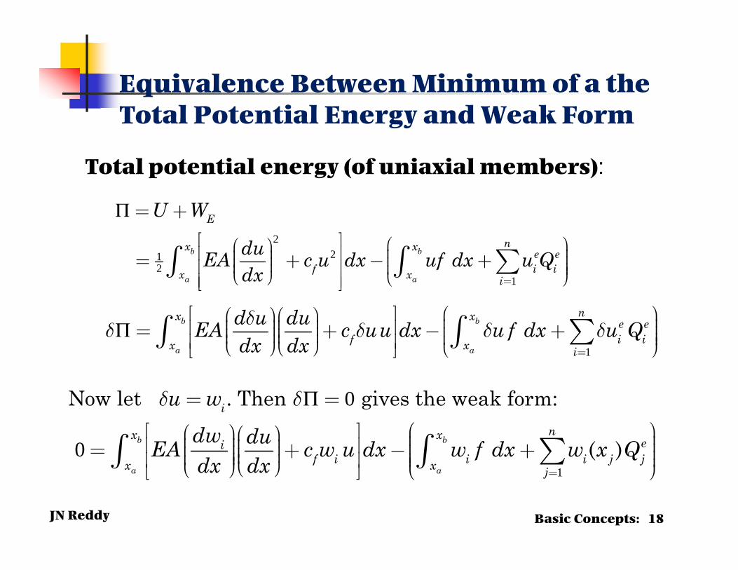
Equivalence Between Minimum of a the Total Potential Energy and Weak Form
Total potential energy (of uniaxial members):
221
21
b b
a a
E
nx x e ef i ix x i
U W
duEA c u dx uf dx u Qdx =
= +
é ù æ öæ ö ÷ê ú÷ çç= + - + ÷÷ çç ÷ê ú÷ç ÷çè ø è øê úë ûåò ò
Π
1
b b
a a
nx x e ef i ix x i
d u duEA c uu dx u f dx u Qdx dxd
d d d d=
é ù æ öæ öæ ö ÷÷ ÷ çç çê ú= + - + ÷÷ ÷ çç ç ÷÷ ÷ç ç ÷çê úè øè ø è øë ûåò òΠ
0Now let . Then gives the weak form:iu wd d= =Π
Basic Concepts: 18
1
0 ( )b b
a a
nx x eif i i i j jx x j
dw duEA c w u dx w f dx w x Qdx dx =
æ öé ùæ öæ ö ÷ç÷ ÷ç çê ú ÷= + - +÷ ç÷ç ç ÷÷ ÷ ççê ú÷ç ÷çè øè ø è øë ûåò ò
JN Reddy
22
0
12
dd d d d
dd d d d
d d
d
é ùê ú= + - - -ê úë û
é ù é ùê ú= + - + +ê úê ú ê úë ûë û
é ùæ ö é ùê ú÷ç= + - + +÷ ê úçê ú÷ç ê úè ø ë ûê úë û
=
ò
ò ò
ò ò
a
a
a
( ) ( )
( ) ( )
( ) ( )
b
a
b a
a b
b a
a b
x
a b bx
x x
a b bx x
x x
a b bx x
d u dua c uu u f dx u x Q u x Qdx dx
d u dua c uu dx u f dx u x Q u x Qdx dx
dua cu dx u f dx u x Q u x Qdx
[ ]12
12
d- =
= -
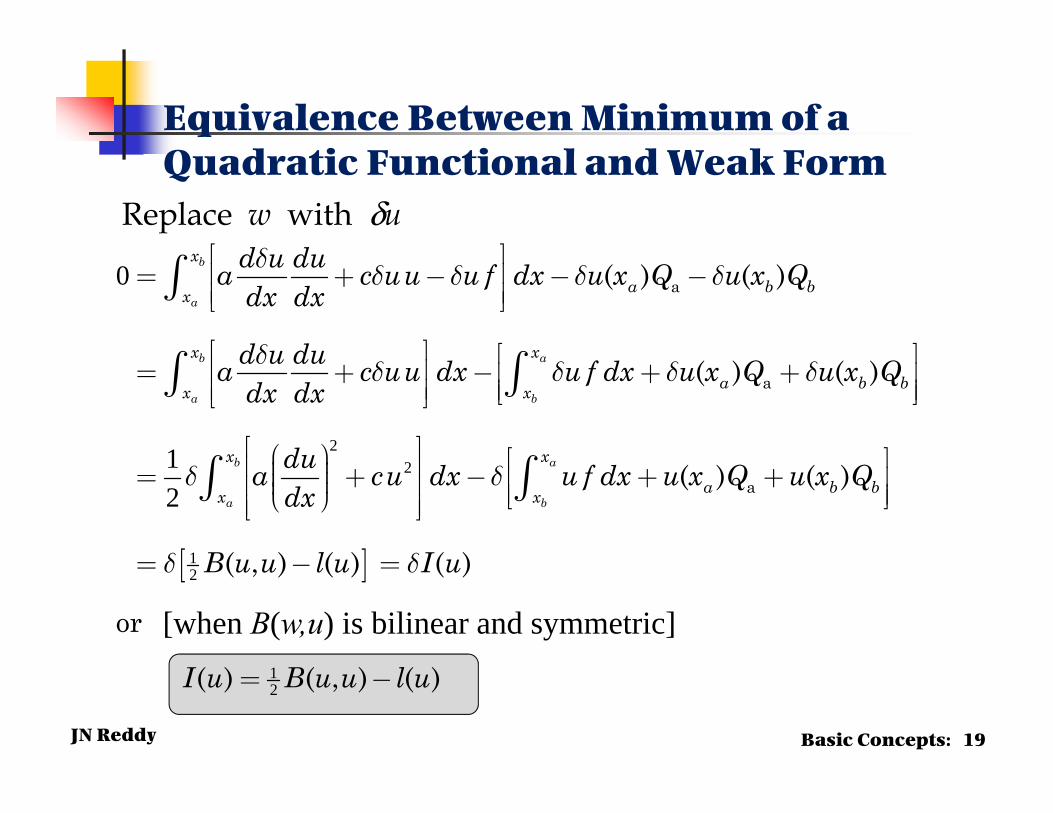
( , ) ( ) ( )
or
( ) ( , ) ( )
B u u l u I u
I u B u u l u
Equivalence Between Minimum of a Quadratic Functional and Weak Form
Replace w with δu
Basic Concepts: 19
[when B(w,u) is bilinear and symmetric]

JN Reddy
FINITE ELEMENT MODEL
1( ) ( ) ( )
ne e eh j j
ju x u x u x
=
≈ = yFinite element approximation
11
0 a( ) ( )
( ) ( )
b a
a b
b a
a b
x xi h
i h i i a i b bx x
n x xj e eij i j i i a i b n
x xj
dw dua cw u dx w f dx w x Q w x Qdx dx
ddu a c dx f dx x Q x Qdx dx
yyy y y y y
=
é ùæ öç ÷ ê ú= + - + + ⋅ç ÷ ê úç ÷ç ÷è ø ë ûé ù é ùê ú ê ú= + - + +ê ú ê úê ú ë ûë û
ò ò
å ò ò
he
211eQ e
nQsF cu=
( )f x
( )= ( )ei iw x xy
Basic Concepts: 20
(is a set of algebraic relations between the primaryand the secondary variables at the nodes)
1 2 2
1
1
[ ]{ } {
(
}
( , ) ,
( ) ( ) ( ))
b
a
b
a
ne e e e e eij j i
j
eex je e eiij i j e e
e e
i jx
xe e e e ei i e i i ii n nx
K u F K u F
ddK B a c dxdx dx
F l f dx x Q x Qx Q
yyy y y
y y
y
y y y
=
= =
= = +
= = + ++ +
JN Reddy
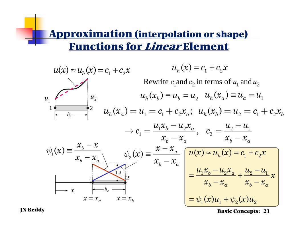
Approximation (interpolation or shape) Functions for Linear Element
1 1 2 2 1 2( ) ; ( )h a a h b bu x u c c x u x u c c x= = + = = +
1 2 2 11 2,b a
b a b a
u x u x u uc cx x x x
- - = =
- -
1 2
1 2 2 1
1 1 2 2
( ) ( )
( ) ( )
h
b a
b a b a
u x u x c c x
u x u x u u xx x x x
x u x u
≈ = +
− −= +− −
= +y y
1 2( ) ( )hu x u x c c x≈ = +
he
21
2u1u
he
21
1( ) b
b a
x xxx x
y−
≡− 2( ) a
b a
x xxx x
y−
≡−
xaxx = bxx =
1.0
1 2( )hu x c c x= +
1( )h a au x u u≡ =2( )h b bu x u u≡ =1 2 1 2Rewrite and in terms of andc c u u
Basic Concepts: 21
JN Reddy
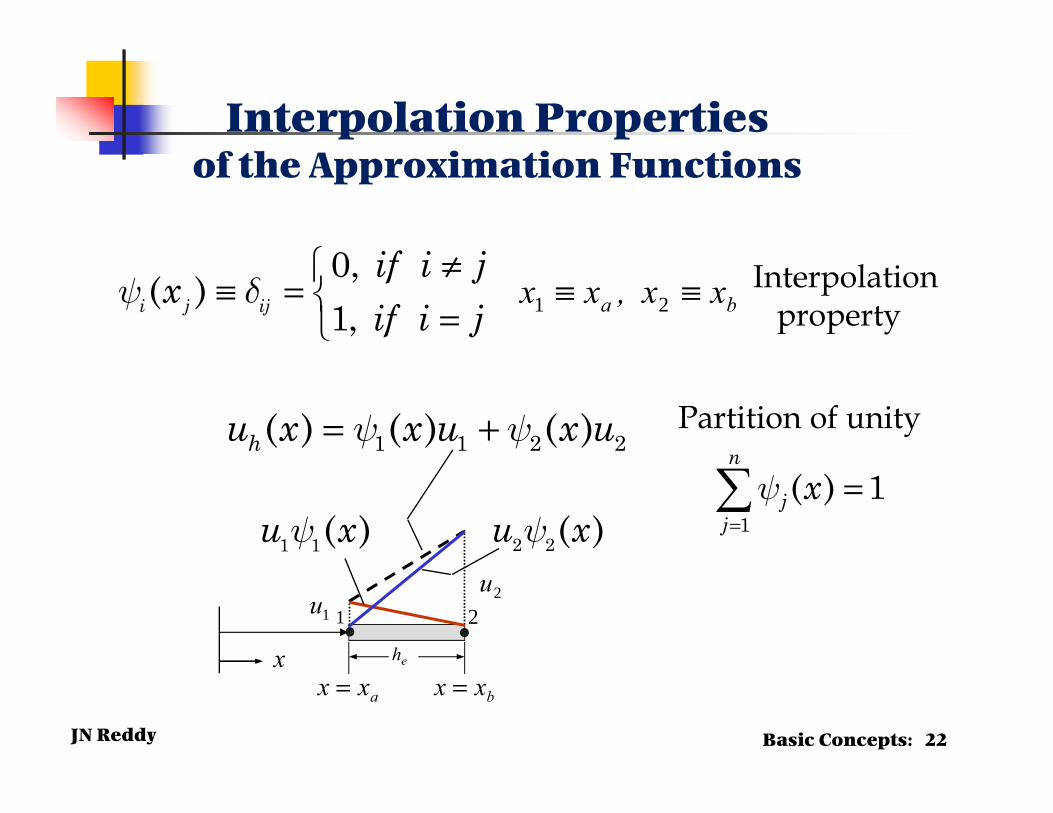
Interpolation Propertiesof the Approximation Functions
2u
he
21
1 1( )u xy 2 2( )u xy
xaxx = bxx =
1u
1 1 2 2( ) ( ) ( )hu x x u x u= +y y
0,( )
1,i j ij
if i jx
if i j≠
≡ = =y d ba xx,xx ≡≡ 21
Interpolation property
1( ) 1
n
jj
x=
=y
Partition of unity
Basic Concepts: 22
JN Reddy
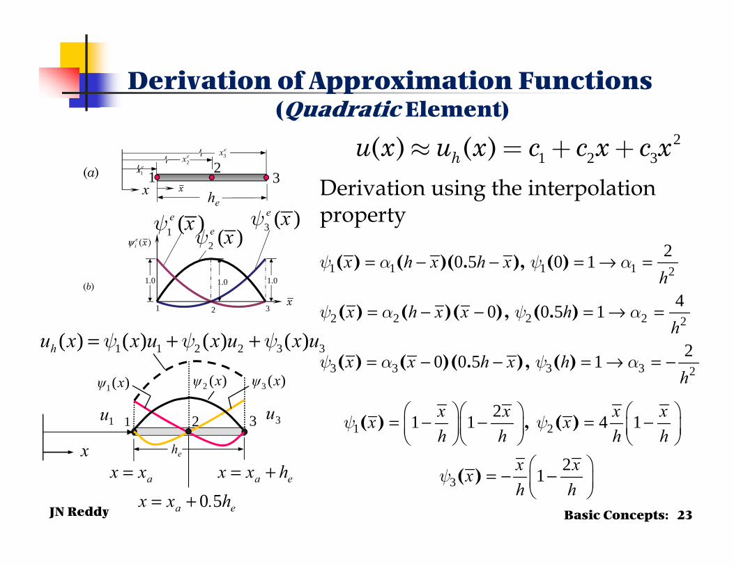
Derivation of Approximation Functions(Quadratic Element)
1 1 1 1 2
2 2 2 2 2
3 3 3 3 2
20 5 0 1
40 0 5 1
20 0 5 1
( ) ( )( . ), ( )
( ) ( )( ), ( . )
( ) ( )( . ), ( )
x h x h xh
x h x x hh
x x h x hh
= − − = → =
= − − = → =
= − − = → = −
y a y a
y a y a
y a y a
Derivation using the interpolation property
he
21
xaxx = ea hxx +=
1u
1 1 2 2 3 3( ) ( ) ( ) ( )hu x x u x u x u= + +y y y
ea h.xx 50+=
3
)(xψ1 )(xψ3)(xψ2
3u
1.0 1.01.0(b)
1 2 3
1 ( )e xy2 ( )e xy
3 ( )e xy
x
)(xeiψ
1 23
x he
(a)
ex3ex2ex1
x
21 2 3( ) ( )hu x u x c c x c x» = + +
1 2
3
21 1 4 1
21
( ) , ( )
( )
x x x xx xh h h h
x xxh h
= − − = −
= − −
y y
y
Basic Concepts: 23
JN Reddy
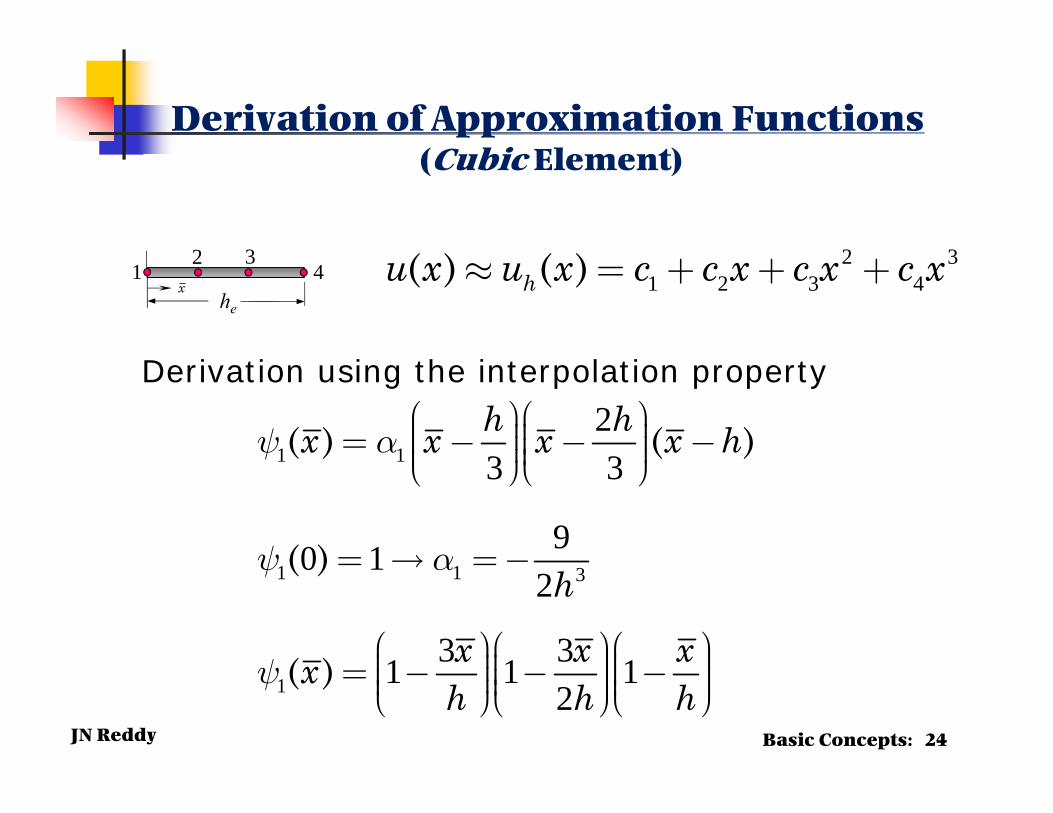
Derivation of Approximation Functions(Cubic Element)
1 1
1 1 3
1
23 3
90 12
3 31 1 12
( ) ( )
( )
( )
h hx x x x h
h
x x xxh h h
æ öæ ö÷ ÷ç ç= - - -÷ ÷ç ç÷ ÷ç çè øè ø
= =-
æ öæ öæ ö÷ ÷ ÷ç ç ç= - - -÷ ÷ ÷ç ç ç÷ ÷ ÷ç ç çè øè øè ø
y a
y a
y
Derivation using the interpolation property
2 31 2 3 4( ) ( )hu x u x c c x c x c x» = + + +1
2 3
hex
4
Basic Concepts: 24
JN Reddy Introduction: 25
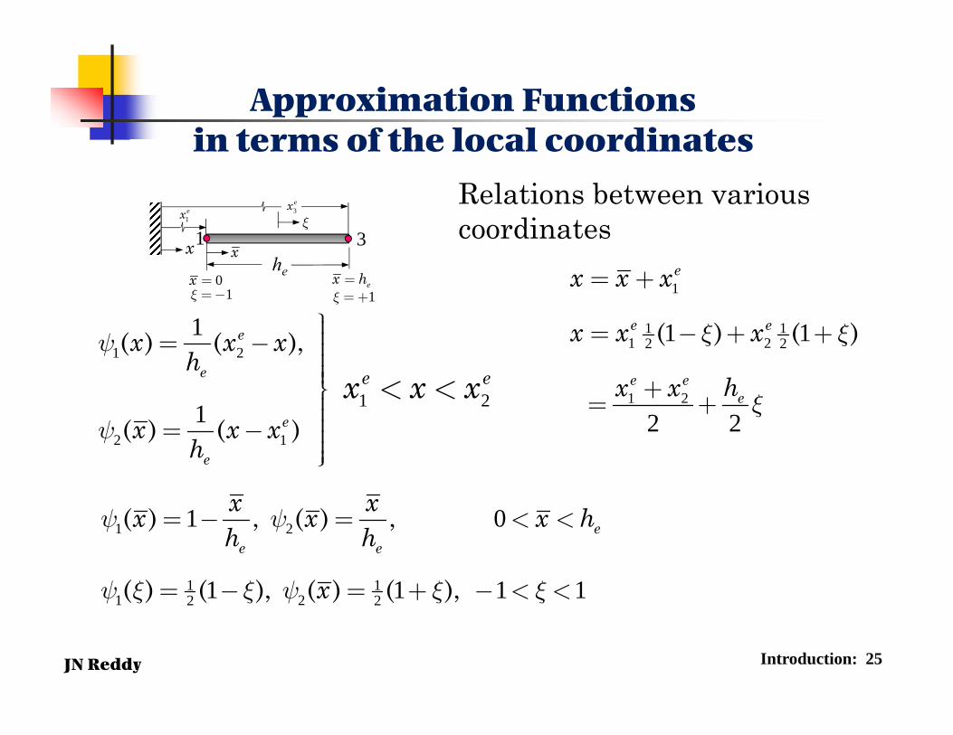
Approximation Functions in terms of the local coordinates
1 3xhe
3ex
1ex
x
x
0x = ex h=1x =- 1x =+ 1
1 11 22 2
1 2
1 1
2 2
( ) ( )
e
e e
e ee
x x x
x x x
hx x
x x
x
= +
= - + +
+= +
Relations between various coordinates
1 2
1 11 22 2
1 0
1 1 1 1
( ) , ( ) ,
( ) ( ), ( ) ( ),
ee e
x xx x x hh h
x
y y
y x x y x x
= - = < <
= - = + - < <
1 2
2 1
1
1
( ) ( ),
( ) ( )
e
e
e
e
x x xh
x x xh
y
y
üïï= - ïïïïýïïï= - ïïïþ
1 2e ex x x< <
JN Reddy Introduction: 26
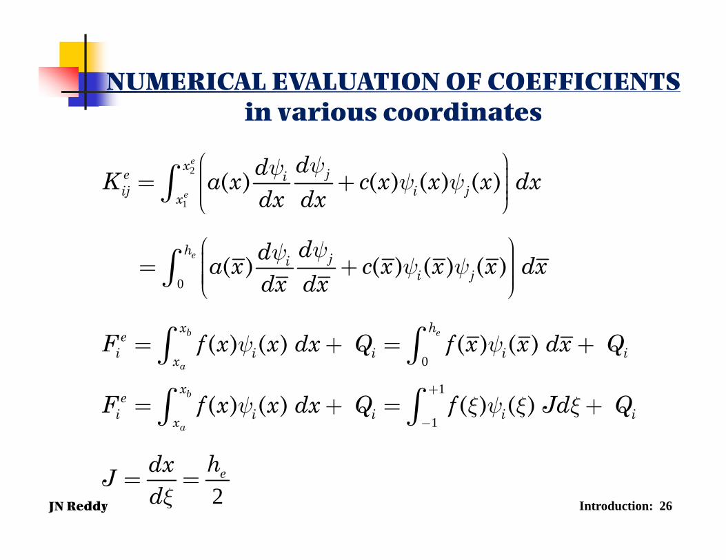
NUMERICAL EVALUATION OF COEFFICIENTSin various coordinates
2
1
0
0
( ) ( ) ( ) ( )
( ) ( ) ( ) ( )
( ) ( ) ( ) ( )
e
e
e
b e
a
x je iij i jx
h jii j
x hei i i i ix
ddK a x c x x x dxdx dx
dda x c x x x dxdx dx
F f x x dx Q f x x dx Q
yyy y
yyy y
y y
æ ö÷ç ÷= +ç ÷ç ÷çè ø
æ ö÷ç ÷= +ç ÷ç ÷çè ø
= + = +
ò
ò
ò ò1
1
2
( ) ( ) ( ) ( ) b
a
xei i i i ix
e
F f x x dx Q f Jd Q
hdxJd
y x y x x
x
+
-= + = +
= =
ò ò
JN Reddy Introduction: 27
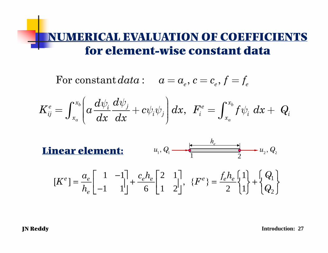
NUMERICAL EVALUATION OF COEFFICIENTSfor element-wise constant data
For constant : , ,
, b b
a a
e e e
x xje eiij i j i i ix x
data a a c c f f
ddK a c dx F f dx Qdx dx
= = =
æ ö÷ç ÷= + = +ç ÷ç ÷çè øò òyy
yy y
1
2
1 1 2 1 11 1 1 2 16 2
[ ] , { }e ee e e e e
e
Qa c h f hK FQh
− = + = + −
Linear element:eh
1 2 2 2,u Q1 1,u Q
JN Reddy
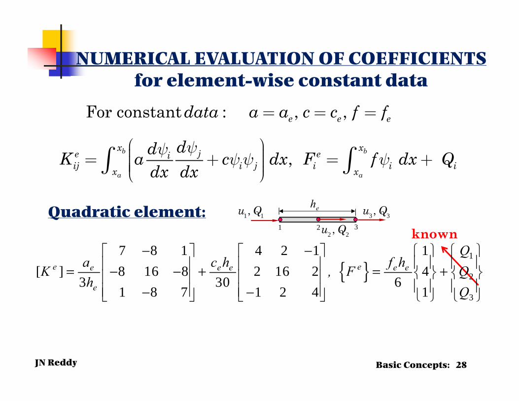
NUMERICAL EVALUATION OF COEFFICIENTSfor element-wise constant data
known
Basic Concepts: 28
{ }1
2
3
7 8 1 4 2 1 1[ ] 8 16 8 2 16 2 4
3 30 61 8 7 1 2 4 1
e ee e e e e
e
Qa c h f hK , F Qh
Q
− − = − − + = + − −
Quadratic element: eh
1 2 31 1,u Q 3 3,u Q
2 2,u Q
For constant : , ,
, b b
a a
e e e
x xje eiij i j i i ix x
data a a c c f f
ddK a c dx F f dx Qdx dx
= = =
æ ö÷ç ÷= + = +ç ÷ç ÷çè øò òyy
yy y
JN Reddy Introduction: 29
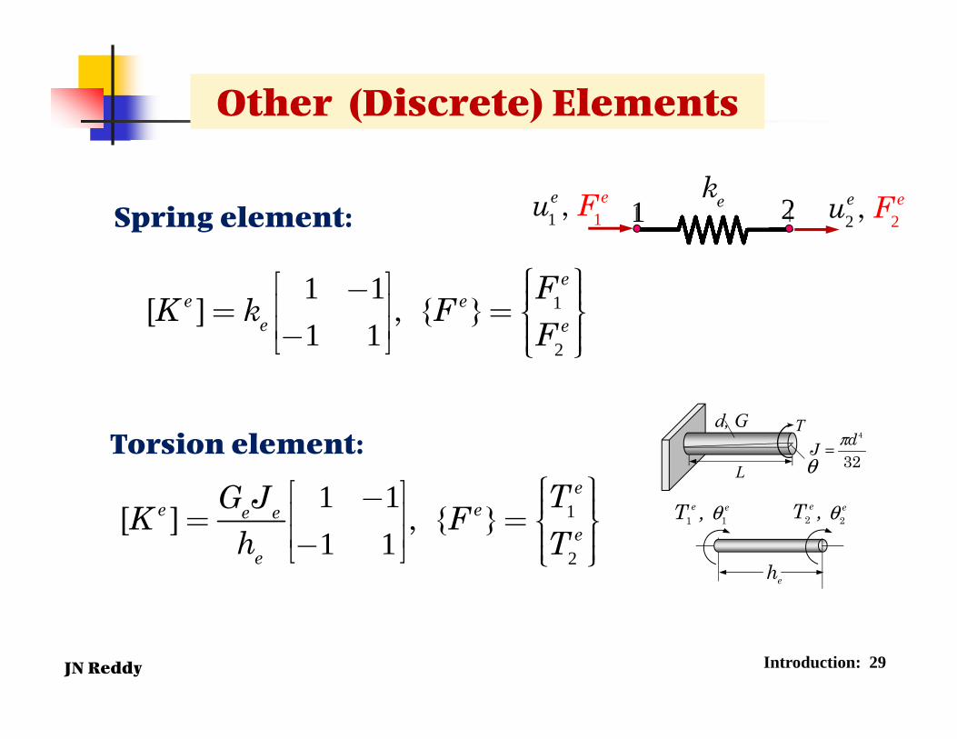
Other (Discrete) Elements
Td, GB
LSteel •
32
4dJ π=θ
e1θ,T e
1e2θ,T e
2
eh
Torsion element:
1
2
1 11 1
[ ] , { }e
e ee ee
e
TG JK Fh T
ì üé ù ï ï- ï ïê ú= = í ýê ú ï ï-ë û ï ïî þ
1
2
1 11 1
[ ] , { }e
e ee e
FK k FF
ì üé ù ï ï- ï ïê ú= = í ýê ú ï ï-ë û ï ïî þ
Spring element: 1 2ek11 ,e eu F
22 ,e eu F

JN Reddy Introduction: 30
1
2
1 11 1
[ ] , { }e
e ee e
IK k FI
ì üé ù ï ï- ï ïê ú= = í ýê ú ï ï-ë û ï ïî þ
Electrical element:1
ee
kR
= 1 2
Electrical resistance
eR =
eR
2 2,e eV I1 1,e eV I
Pipe flow element:
1
2
1 11 1
[ ] , { }e
e ee e
QK k FQì üé ù ï ï- ï ïê ú= = í ýê ú ï ï-ë û ï ïî þ
4
128ee
dkh
pm
=
d 1 1,e eP Q
eh
2 2,e eP Q
Other (Discrete) Elements (continued)
JN Reddy
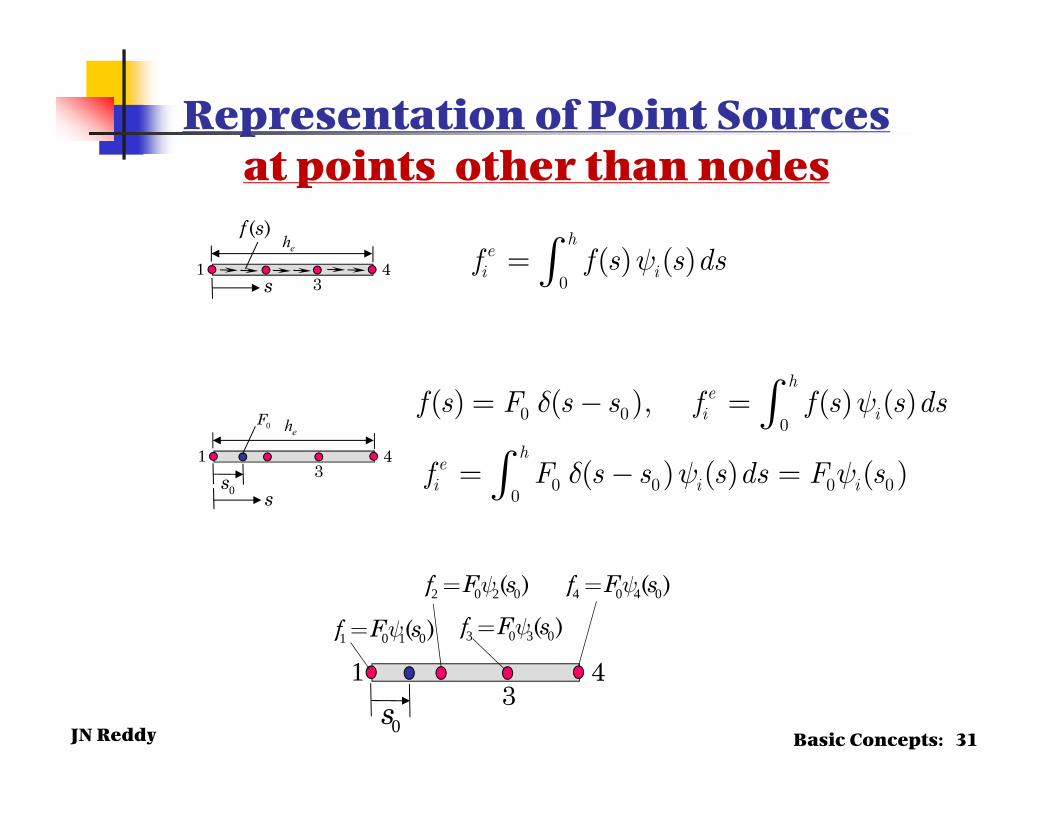
Representation of Point Sourcesat points other than nodes
1 41 0 1 0( )f F sy=
0s3
2 0 2 0( )f F sy=
3 0 3 0( )f F sy=
4 0 4 0( )f F sy=
0( ) ( )
hei if f s s dsy= ò
eh
1 4
( )f s
s 3
eh
1 4
0F
s0s 3
0 00
0 0 0 00
( ) ( ), ( ) ( )
( ) ( ) ( )
hei i
hei i i
f s F s s f f s s ds
f F s s s ds F s
d y
d y y
= - =
= - =
ò
ò
Basic Concepts: 31
JN Reddy Basic Concepts: 32
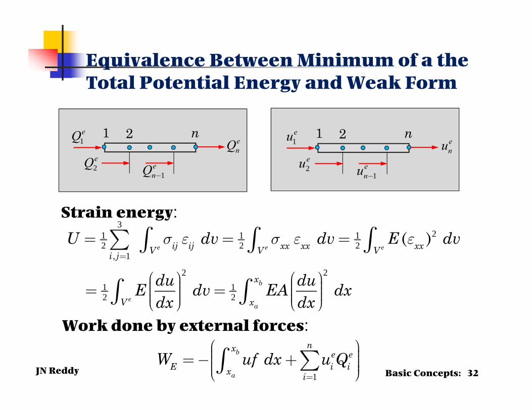
Equivalence Between Minimum of a the Total Potential Energy and Weak Form
321 1 1
2 2 21
2 21 12 2
,( )
e e e
b
ea
ij ij xx xx xxV V Vi j
x
V x
U dv dv E dv
du duE dv EA dxdx dx
s e s e e=
= = =
æ ö æ ö÷ ÷ç ç= =÷ ÷ç ç÷ ÷ç çè ø è ø
å ò ò ò
ò ò
Strain energy:
enQ1
eQ 21 n
2eQ
1-enQ
enu1
eu 21 n
2eu
1-enu
Work done by external forces:
1
b
a
nx e eE i ix i
W uf dx u Q=
æ ö÷ç=- + ÷ç ÷ç ÷è øåò
JN Reddy
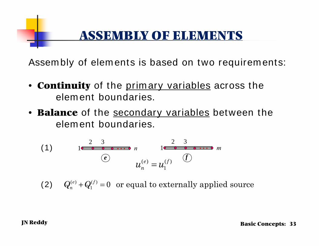
ASSEMBLY OF ELEMENTS
Assembly of elements is based on two requirements:
• Continuity of the primary variables across theelement boundaries.
• Balance of the secondary variables between theelement boundaries.
(1) 12 3 … n
e1
2 3 … mf
( ) ( )1
e fnu u=
(2) ( ) ( )1 0 or equal to externally applied sourcee f
nQ Q+ =
Basic Concepts: 33
JN Reddy
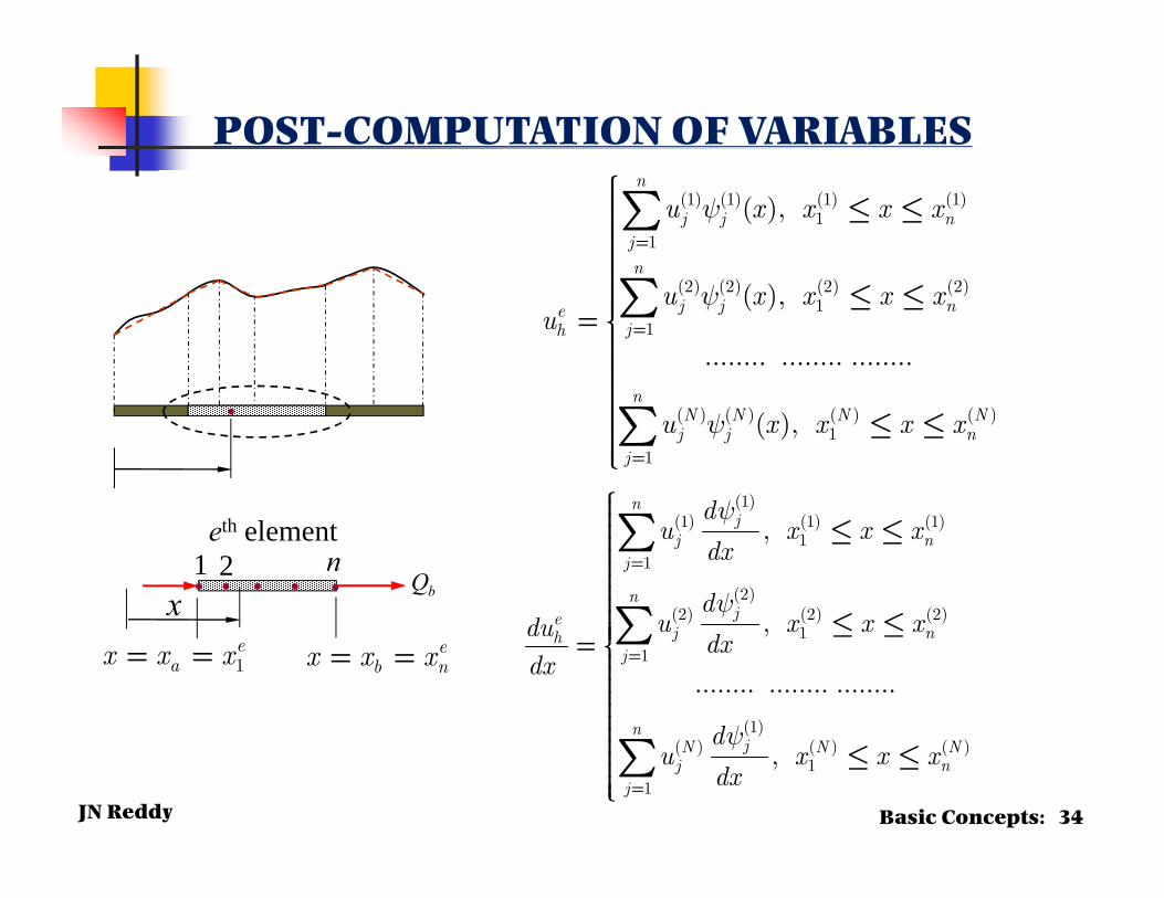
POST-COMPUTATION OF VARIABLES(1) (1) (1) (1)
11
(2) (2) (2) (2)1
1
( ) ( ) ( ) ( )1
1
( ),
( ),
........ ........ ........
( ),
n
j j nj
n
j j nejh
nN N N Nj j n
j
u x x x x
u x x x xu
u x x x x
y
y
y
=
=
=
ìïï £ £ïïïïïïï £ £ïï= íïïïïïïï £ £ïïïïî
å
å
åx
aQbQ
1e
ax x x= = eb nx x x= =
• • •• •1 2 n
x
eth element
•
(1)(1) (1) (1)
11
(2)(2) (2) (2)
11
(1)( ) ( ) ( )
11
,
,
........ ........ ........
,
nj
j nj
nje
j nhj
njN N N
j nj
du x x xdx
du x x xdudx
dx
du x x x
dx
y
y
y
=
=
=
ìïï £ £ïïïïïïïï £ £ïï= íïïïïïïïï £ £ïïïïî
å
å
åBasic Concepts: 34
JN Reddy
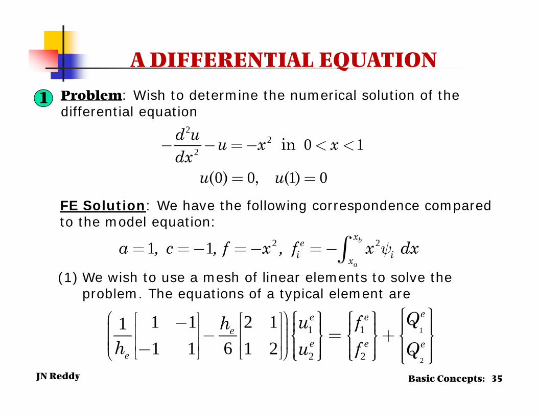
A DIFFERENTIAL EQUATION
FE Solution: We have the following correspondence compared to the model equation:
2 21 1= =- =- =-òb
a
xei ix
a , c , f x , f x dxy
(1) We wish to use a mesh of linear elements to solve the problem. The equations of a typical element are
1
2
1 1
2 2
1 1 2 1161 1 1 2
ì üï ïì ü ì üæ öé ù é ù ï ï ï ï- ï ï÷ï ï ï ï ï ïç ê ú ê ú÷- = +ç í ý í ý í ý÷ç ê ú ê ú÷ï ï ï ï ï ïç -è øë û ë û ï ï ï ï ï ïî þ î þ ï ïî þ
ee ee
e e ee
Qu fhh u f Q
Basic Concepts: 35
Problem: Wish to determine the numerical solution of the differential equation
22
2 0 1
0 0 1 0
in
( ) , ( )
d u u x xdx
u u
- - =- < <
= =
1
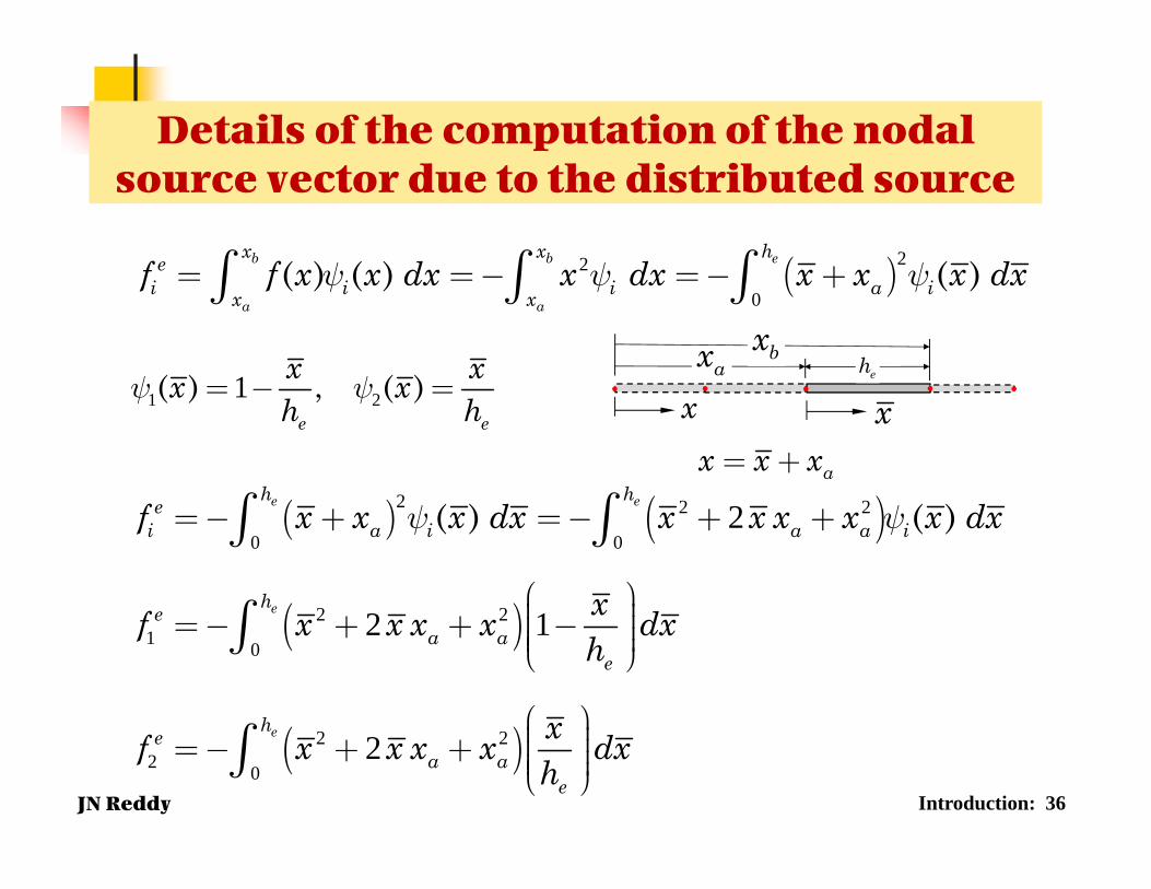
JN Reddy Introduction: 36
( )22
0y y y= =- =- +ò ò ò( ) ( ) ( )b b e
a a
x x hei i i a ix x
f f x x dx x dx x x x dx
Details of the computation of the nodal source vector due to the distributed source
● ● ●●●
x xax bx
eh
= + ax x x
1 21( ) , ( )e e
x xx xh h
y y= - =
( ) ( )
( )
( )
2 2 2
0 0
2 21 0
2 22 0
2
2 1
2
y y=- + =- + +
æ ö÷ç ÷=- + + -ç ÷ç ÷çè ø
æ ö÷ç ÷=- + + ç ÷ç ÷çè ø
ò ò
ò
ò
( ) ( )e e
e
e
h hei a i a a i
hea a
e
hea a
e
f x x x dx x x x x x dx
xf x x x x dxh
xf x x x x dxh
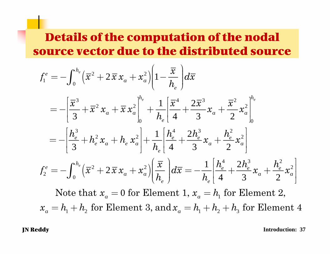
JN Reddy Introduction: 37
Details of the computation of the nodal source vector due to the distributed source
( )
( )
2 21 0
3 4 3 22 2 2
0 0
3 4 3 22 2 2
42 2
2 0
2 1
1 23 4 3 2
213 4 3 2
12
æ ö÷ç ÷=- + + -ç ÷ç ÷çè ø
é ù é ùê ú ê ú=- + + + + +ê ú ê úë û ë ûé ù é ùê ú ê ú=- + + + + +ê ú ê úë û ë û
æ ö÷ç ÷=- + + =-ç ÷ç ÷çè ø
ò
ò
e
e e
e
hea a
e
h h
a a a ae
e e e ee a e a a a
e
he ea a
e e
xf x x x x dxh
x x x xx x x x x xh
h h h hh x h x x xh
hxf x x x x dxh h
3 22
1
1 2 1 2 3
24 3 2
0
é ùê ú+ +ê úë û
= =
= + = + +
Note that for Element 1, for Element 2,for Element 3, and for Element 4
e ea a
a a
a a
h hx x
x x hx h h x h h h

JN Reddy
(2) We consider a mesh of 4 linear elements (h =0.25). The element equations are 1 2 3 4 5
1 2 3 4
1
+
−=
−
−1
1
1
1
241
2
1
2
1
003910001300
94979794
.
.uu
1 2)(1
1Q )(12Q
+
−=
−
−2
2
2
2
241
2
1
2
1
022320014320
94979794
.
.uu
1 22)(2
1Q )(22Q
+
−=
−
−3
3
3
3
241
2
1
2
1
055990042970
94979794
.
.uu
1 23)(3
1Q )(32Q
+
−=
−
−4
4
4
4
241
2
1
2
1
105470087240
94979794
.
.uu
1 24)(4
1Q )(42Q
Basic Concepts: 38
A DIFFERENTIAL EQUATION (cont.)
JN Reddy
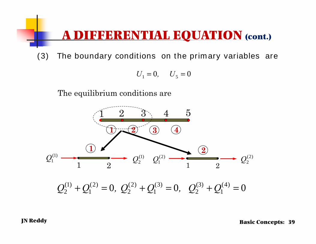
(3) The boundary conditions on the primary variables are
(1) (2) (2) (3) (3) (4)2 1 2 1 2 10 0 0Q Q , Q Q , Q Q+ = + = + =
00 51 == U,U
1 2 3 4 51 2 3 4
1 2
1)(1
1Q )(12Q )(2
1Q )(22Q
2 1
2
The equilibrium conditions are
Basic Concepts: 39
A DIFFERENTIAL EQUATION (cont.)
JN Reddy
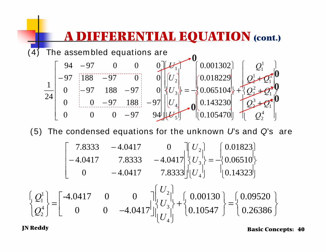
(4) The assembled equations are
+++
+
−=
−−−
−−−−
−
42
41
32
31
22
21
12
11
5
4
3
2
1
94970009718897000971889700097188970009794
241
QQQQQQQ
Q
UUUUU
0.1054700.1432300.0651040.0182290.001302
−=
−−−
−
0.143230.065100.01823
7.83334.041704.0417 7.83334.0417
4.04177.8333
4
3
20
UUU
(5) The condensed equations for the unknown U’s and Q’s are
211
342
4
-4.0417 0 0 0.00130 0.095200 0 4.0417 0.10547 0.26386
UQ
UQ
U
= + = −
000
0
0
Basic Concepts: 40
A DIFFERENTIAL EQUATION (cont.)
JN Reddy
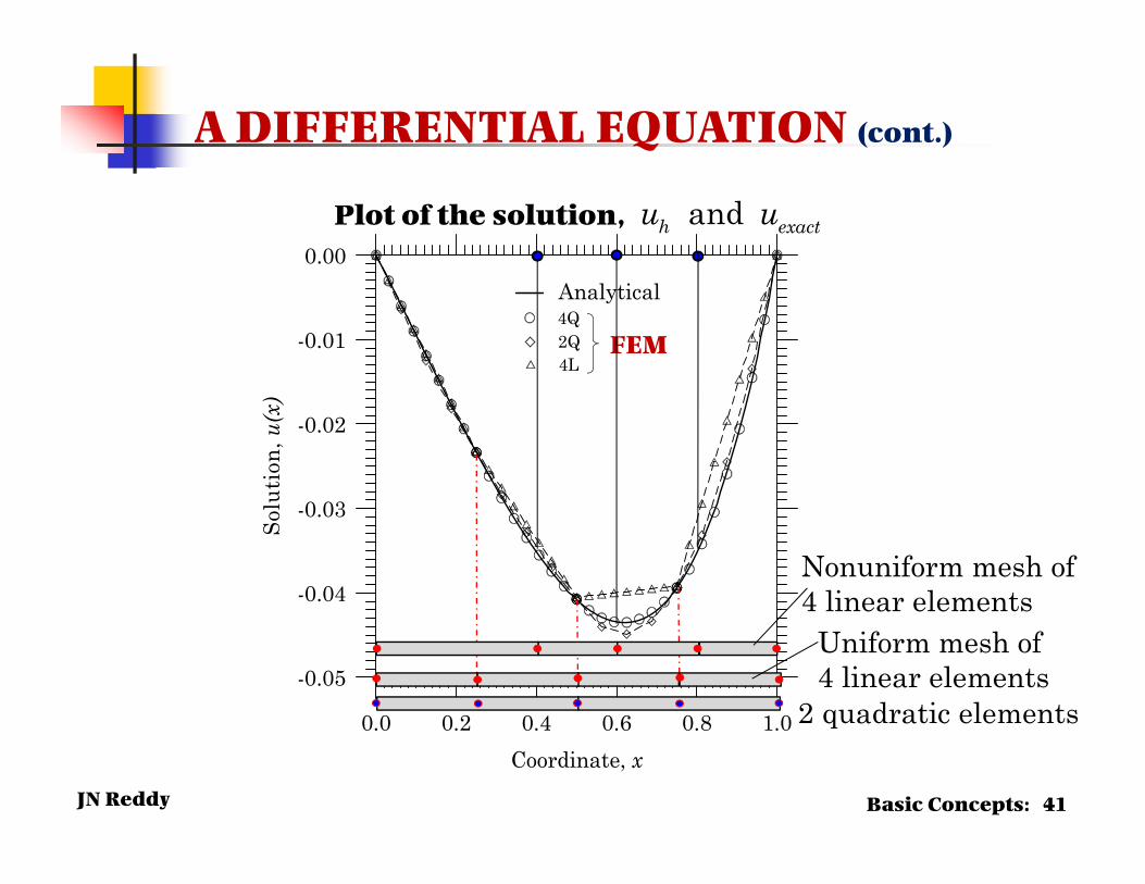
0.0 0.2 0.4 0.6 0.8 1.0Coordinate, x
-0.05
-0.04
-0.03
-0.02
-0.01
0.00So
luti
on, u
(x)
Analytical
4L2Q4Q
Plot of the solution,
Basic Concepts: 41
andh exactu u
FEM
Uniform mesh of 4 linear elements
2 quadratic elements
Nonuniform mesh of 4 linear elements
A DIFFERENTIAL EQUATION (cont.)
JN Reddy
0.0 0.2 0.4 0.6 0.8 1.0Coordinate, x
-0.15
-0.10
-0.05
0.00
0.05
0.10
0.15
0.20
0.25
0.30
Solu
tion
, du/
dx
Analytical
4L2Q4Q
FEM
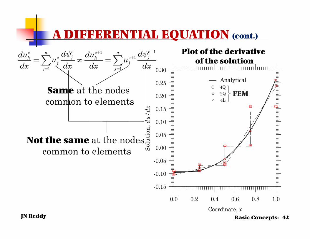
Plot of the derivative of the solution
Basic Concepts: 42
111
1 1
e ee en nj je eh h
j jj j
d ddu duu udx dx dx dx
y y +++
= =
= ¹ =å å
Same at the nodes common to elements
Not the same at the nodes common to elements
A DIFFERENTIAL EQUATION (cont.)
JN ReddyBasic Concepts: 43
Rigid bar
211
°°°°
2
3
4
2
21
2
Global nodes
Element nodes
(2)2 3u U≡
2k
3
(1)1 1u U≡
P
3k
1k
°°°
°
° 1
(3)2 4u U≡
(1) (2) (3)2 1 1 3u u u U= = ≡
2
2
1
ek1 2
e1δ e
2δ
1eF eF2
1
2
1 11 1
[ ] , { }e
e ee e
FK k F
F
− = = −
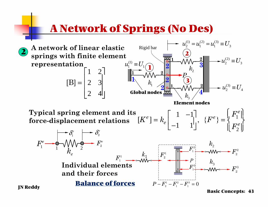
Typical spring element and its force-displacement relations
A network of linear elasticsprings with finite element representation
k1°°
11F
12F
31F
P
°°°
°°°°
°
°
21F
°°2
2F
°°3
2F
031
21
12 =−−− FFFP
2k
3kIndividual elements and their forces
Balance of forces
1 22 32 4
[B] =
A Network of Springs (No Des)
2
JN Reddy
Rigid bar
211
°°°°
2
3
4
2
21
2
Global nodes
Element nodes
2U3U
4U
2k
3
1U
P
3k
1k
°°°
°
°1
1 °
°
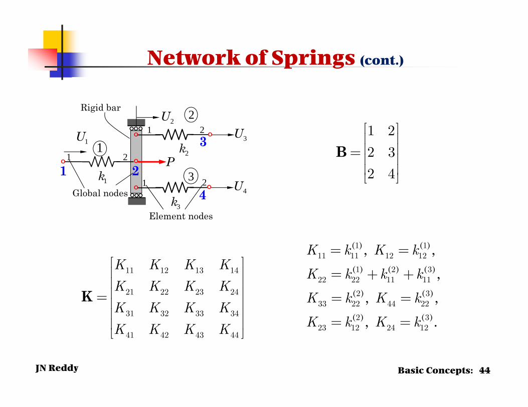
°B
é ùê úê ú= ê úê úë û
1 2
2 3
2 4
K
K K K K
K K K K
K K K K
K K K K
é ùê úê úê ú= ê úê úê úë û
11 12 13 14
21 22 23 24
31 32 33 34
41 42 43 44
( ) ( )
( ) ( ) ( )
( ) ( )
( ) ( )
, ,,
, ,, .
K k K k
K k k k
K k K k
K k K k
= =
= + +
= =
= =
1 111 11 12 12
1 2 322 22 11 11
2 333 22 44 22
2 323 12 24 12
Basic Concepts: 44
Network of Springs (cont.)
JN Reddy
0
00
P
1 11 1
1 1 12 2
1 11 1
( ) ( )
( ) ( )
u Fk
u F
− = −
2 21 1
2 2 22 2
1 11 1
( ) ( )
( ) ( )
u Fk
u F
− = −
3 31 1
3 3 32 2
1 11 1
( ) ( )
( ) ( )
u Fk
u F
− = −
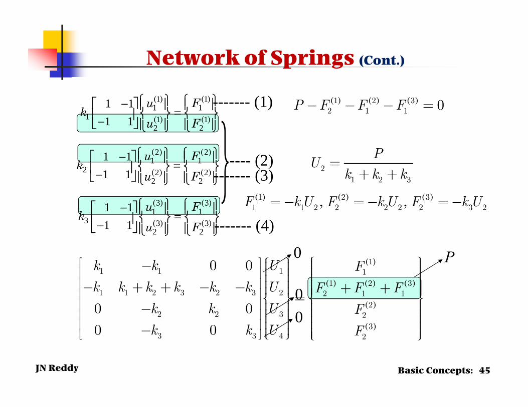
( ) ( ) ( )P F F F- - - =1 2 32 1 1 0------- (1)
---- (2)------- (3)
------- (4)
( )
( ) ( ) ( )
( )
( )
k k U F
k k k k k k U F F F
k k U F
k k U F
ì üé ù ì ü- ï ïï ï ï ïï ïê ú ï ïï ïê ú ï ïï ï- + + - - + +ï ïï ï ï ïê ú =í ý í ýê ú ï ï ï ï- ï ï ï ïê ú ï ï ï ïê ú ï ï ï ï- ï ï ï ïë û î þ ï ïî þ
11 1 1 1
1 2 31 1 2 3 2 3 2 2 1 1
22 2 3 2
33 3 4 2
0 0
0 0
0 0
PU
k k k=
+ +21 2 3
( ) ( ) ( ), ,F kU F kU F kU=- =- =-1 2 31 1 2 2 2 2 2 3 2
Basic Concepts: 45
Network of Springs (Cont.)
JN Reddy
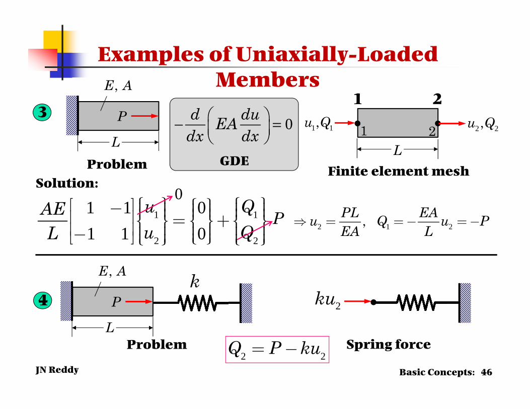
Examples of Uniaxially-Loaded Members
2 1 2,PL EAu Q u PEA L
= =- =-
P
,E A
Problem
L
1 1
2 2
1 1 01 1 0
u QAEu QLì ü ì üé ù ì üï ï ï ï- ï ïï ï ï ï ï ïê ú = +í ý í ý í ýê ú ï ï ï ï ï ï- ï ïë û î þï ï ï ïî þ î þ
• •1 2
1 2
Finite element mesh
L
1 1,u Q 2 2,u Q
0P
P
,E A
ProblemL
k
Spring force
2ku •
Basic Concepts: 46
2 2Q P ku= -
Solution:
3
4
0d duEAdx dx
− =
GDE
JN Reddy
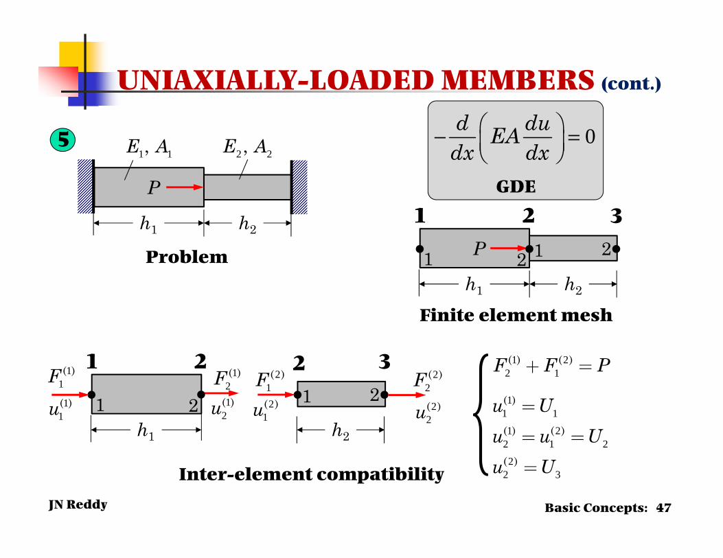
UNIAXIALLY-LOADED MEMBERS (cont.)
P
1 1,E A 2 2,E A
h1 h2
Problem P
h1 h2
• • •1 2 1 21 2 3
Finite element mesh
Inter-element compatibility
h1 h2
• • •1 2 1 21 2 32
•1
1( )F 1
2( )F 2
1( )F 2
2( )F
11( )u 1
2( )u 2
1( )u 2
2( )u
1 22 1( ) ( )F F P+ =
11 11 2
2 1 22
2 3
( )
( ) ( )
( )
u Uu u Uu U
=
= =
=
Basic Concepts: 47
5 0d duEAdx dx
− =
GDE
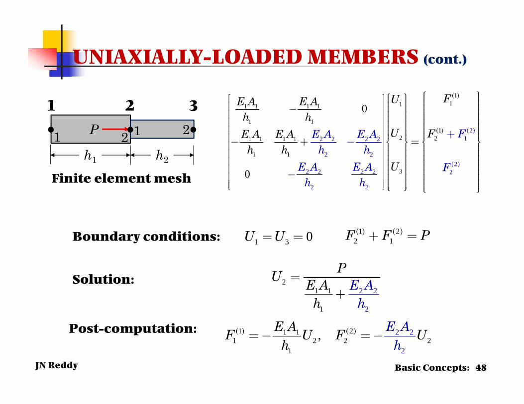
JN Reddy
P
h1 h2
• • •1 2 1 21 2 3
Finite element mesh
212 2 2 2
2 22
2 2 2 2 2
1111 1 1 1
1 11
2 21 1 1 1
1 1
3
2 2
0
0
( )
( )
( )
( ) FE A E Ah h
E A E A Fh
FUE A E Ah h
U FE A E Ah h
Uh
ì üì ü ï ïé ù ï ï ï ïï ïê ú ï ï- ï ï ï ïï ïê ú ï ïï ï ï ïê ú ï ï ï ïï ïê ú ï ïï ï ï ïï ïê ú- + =í ý í ýê ú ï ï ï ïï ï ï ïê ú ï ï ï ïê ú ï ï ï ïï ï ï ïê ú ï ï ï ïï ï ï ïê ú ï ï ï ïê úë û ï ï ï ïî
+-
þ î-
þ
Boundary conditions: 1 3 0U U= = 1 22 1( ) ( )F F P+ =
Solution: 21 21
1
2
2
PU E Ah
E Ah
=+
Post-computation: 1 21 211
2
22 2 2
1
( ) ( ),E A E AF U F Uh h
=- =-
Basic Concepts: 48
UNIAXIALLY-LOADED MEMBERS (cont.)
JN ReddyIntroduction: 49
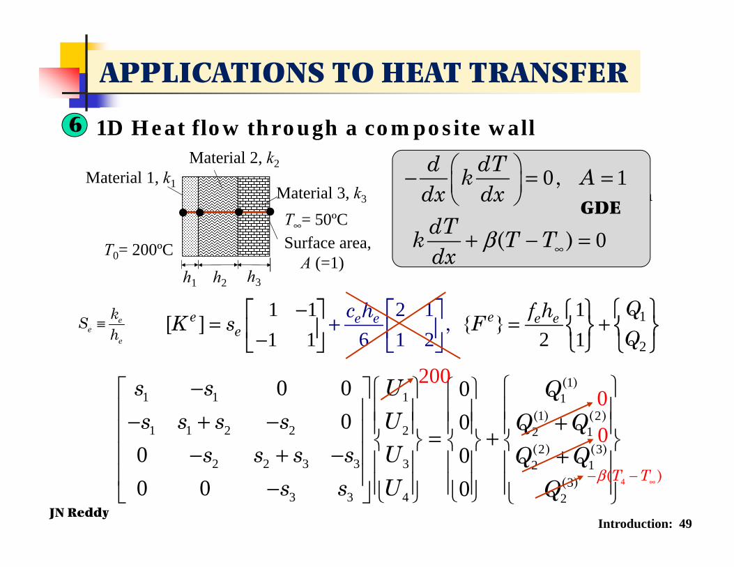
APPLICATIONS TO HEAT TRANSFER
ee
e
kSh
≡ 1
2
1 1 121 1 1
2 16 1 2
[ ] { },e e e eee
e Qf hK c hs FQ
− = = + −
+
50
1 1
2 2
3 32
70 W/(m C), 2 cm 40 W/(m C), 2.5 cm 20 W/(m C), 4 cm
C, 10 W/(m C)
k hk hk hT β∞
= ⋅ =
= ⋅ =
= ⋅ =
= = ⋅
Material 1, k1
Material 2, k2
Material 3, k3
h3h1 h2
Surface area,A (=1)
T∞= 50ºC
T0= 200ºC
● ● ● ●
11 1 1 1
1 21 1 2 2 2 2 1
2 32 2 3 3 3 2 1
33 3 4 2
0 0 00 0
0 00 0 0
( )
( ) ( )
( ) ( )
( )
s s U Qs s s s U Q Q
s s s s U Q Qs s U Q
− − + − + = + − + − + −
2000
0
4( )T Tβ ∞− −
6 1D Heat flow through a composite wall
0 1
0
,
( )
d dTk Adx dxdTk T Tdx
β ∞
− = =
+ − =GDE
JN Reddy
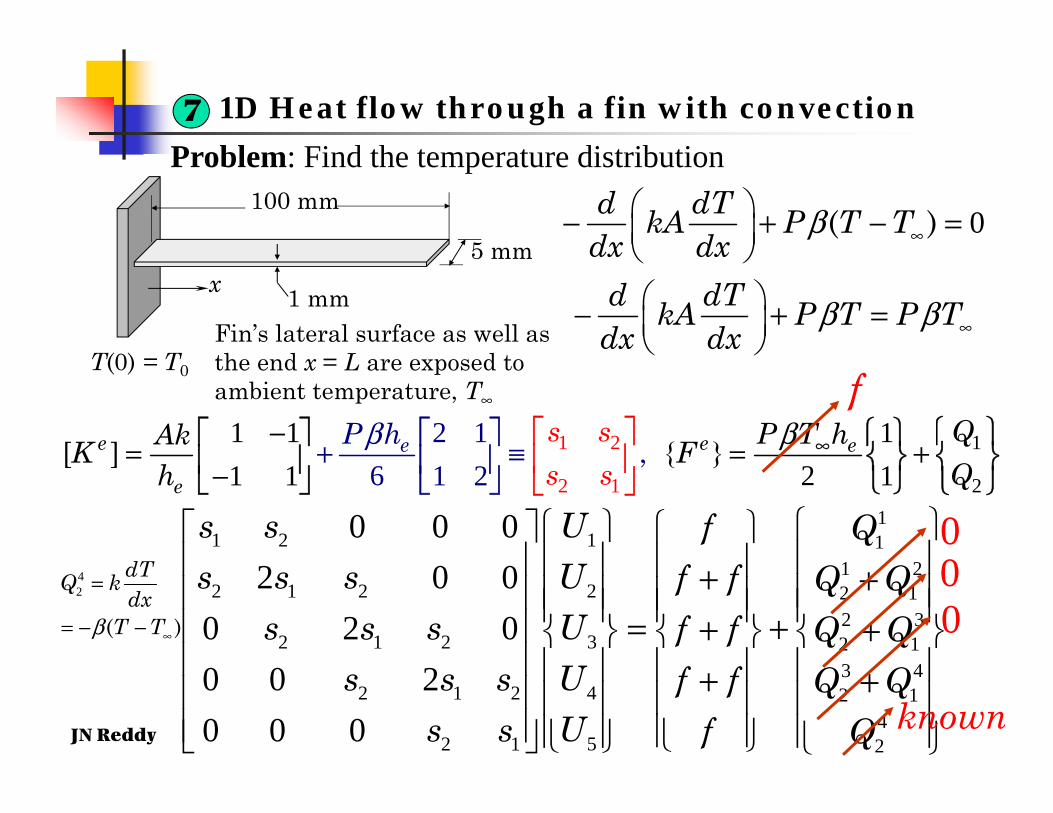
0( )d dTkA P T Tdx dx
d dTkA P T P Tdx dx
β
β β
∞
∞
− + − = − + =
2
2
1
2
1
1
2 11 1 121 1 1 2 16
[ ] { },e ee e
e
s ss
QP T hAkKQs
P Fh
hβ β ∞− = =
+ +
≡
−
f
111 2 1
1 222 1 2 2 1
2 332 1 2 2 1
3 442 1 2 2 1
452 1 2
0 0 02 0 0
0 2 00 0 20 0 0
Us s f QUs s s f f Q QUs s s f f Q QUs s s f f Q QUs s f Q
+ + = + + +
+ +
000
42
( )
dTQ kdx
T Tβ ∞
=
= − −
known
7 1D Heat flow through a fin with convection
Fin’s lateral surface as well as the end x = L are exposed to ambient temperature, T∞
T(0) = T0
100 mm
5 mm
1 mmx
Problem: Find the temperature distribution
JN Reddy Introduction: 51
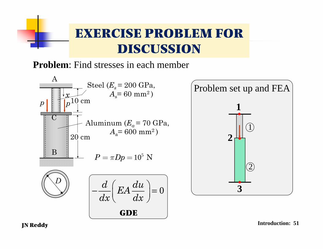
EXERCISE PROBLEM FOR DISCUSSION
1
2
●
●
●
1
2
3
Problem set up and FEA10 cmp
20 cm
Steel (Es = 200 GPa, As= 60 mm2 )
Aluminum (Ea = 70 GPa,Aa= 600 mm2 )
A
C
B
xp
510 NP Dpp= =
D
Problem: Find stresses in each member
0d duEAdx dx
− =
GDE
JN Reddy Introduction: 52
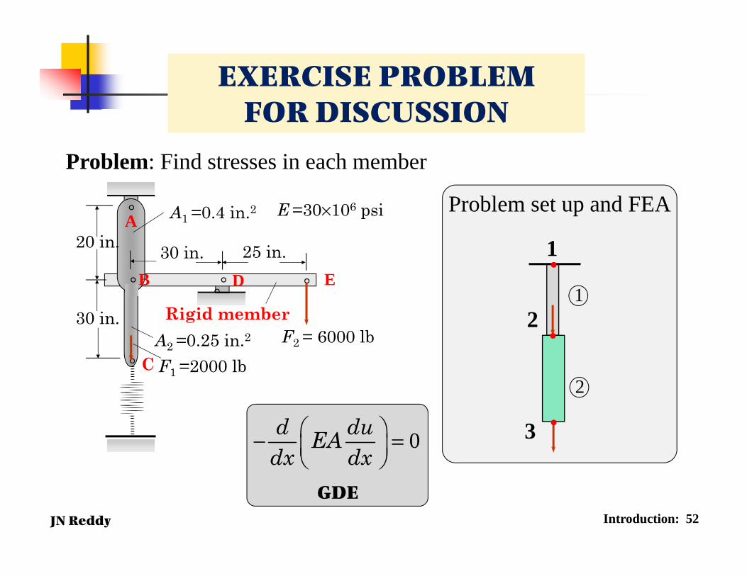
EXERCISE PROBLEM FOR DISCUSSION
Problem set up and FEA
Problem: Find stresses in each member
A2 =0.25 in.2
F1 =2000 lb
Rigid member
°
°
°
°°
A20 in.
B
C
30 in.
30 in. 25 in.E
A1 =0.4 in.2 E =30×106 psi
D°
F2 = 6000 lb
1
2
●
●
●
1
2
30d duEAdx dx
− =
GDE

JN Reddy Introduction: 53
EXERCISE PROBLEM FOR DISCUSSION
2
2
1
1
( )
, ,
,r
r
d trt tr dr r
du u u du Ec c cdr r r d
r
r
q
q
ss rw
s n s nn
- +
æ ö æ ö÷ ÷ç ç= + = + =÷ ÷ç ç÷ ÷ç çè ø è ø -
=GDE:
Problem: Find the hoop stress in the rotating circular disc
●( , )r q
rq
w
2
00
0
10
2
( )
( ) ( )
b
a
b
a
r
rr
r
r a a b br
d tw tr f rdrdr dr r
dwtr wt wf r dr Q w r Q w rdr
pq
q
ss q
p s s
é ùê ú= - + -ê úë û
æ ö÷ç= + - - -÷ç ÷çè ø
ò ò
ò
Weak Form:2
0 2 2, ( ) , ( )a r a b r bf t r Q tr Q trrw p s p s= º - º
JN Reddy Introduction: 54
0
12
2
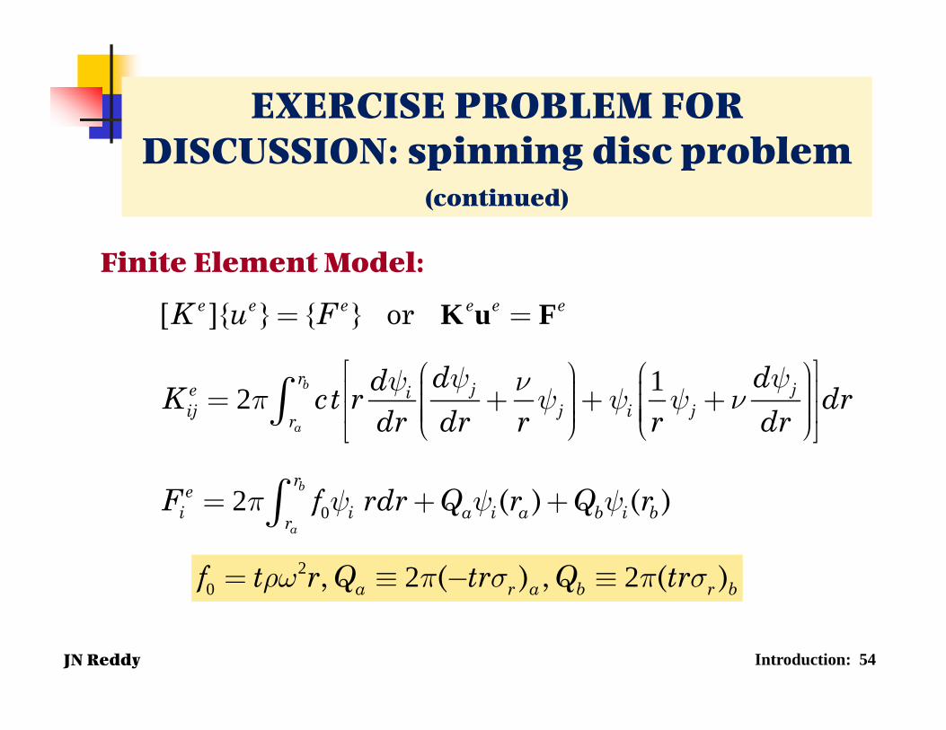
[ ]{ } { } or
( ) ( )
b
a
b
a
e e e e e e
r j je iij j i jr
rei i a i a b i br
K u F
d ddK ct r drdr dr r r dr
F f rdr Q r Q r
y yy np y y y n
p y y y
= =
é ùæ ö æ ö÷ ÷ç çê ú÷ ÷= + + +ç ç÷ ÷ê úç ç÷ ÷ç çè ø è øë û
= + +
ò
ò
K u F
20 2 2, ( ) , ( )a r a b r bf t r Q tr Q trrw p s p s= º - º
EXERCISE PROBLEM FOR DISCUSSION: spinning disc problem
(continued)
Finite Element Model:
JN Reddy
SUMMARY
Beginning with a model second-order differentialequation that arises, for example, in connection withaxial deformation of bars, 1-D heat transfer in fins ofa heat exchanger, or 1-D flow through pipes andchannels, the following steps are used to in the finiteelement analysis of the problem:
1. Divided the domain into subdomains, called finiteelements.
2. Over each element, an integral statement, calledweakform, is developed. The weak form is equivalent tothe differential equation as well as specified naturalboundary conditions on the boundary of the element.
Basic Concepts: 55
JN Reddy
SUMMARY (continued)
3. Using polynomial approximation of the variables, asystem of algebraic equations, called finite elementmodel, is developed. The model relates the nodal valuesof the PVs and the SVs.
4. The element equations are then assembled to eliminateexcessive unknown SVs by requiring continuity of PVsand balance of SVs at the nodes.
5. The assembled system of equations are then solved forthe unknown PVs at the nodes by using the knownboundary conditions.
6. Post-computation may be used to compute SVs and PVs atpoints other than nodes. The SVs are discontinuousbetween elements.
Basic Concepts: 56