Lecture 5

Three level variance component models

Three levels models

• In three levels models the clusters themselves are nested in superclusters, forming a hierarchical structure.

• For example, we might have repeated measurement occasions (units) for patients (clusters) who are clustered in hospitals (superclusters).

Which method is best for

measuring respiratory flow?

• Peak respiratory flow (PEFR) is measured by two methods, the standard Wright peak flow and the Mini Wright meter, each on two occasions on 17 subjects.

Table 1.1: Peak respiratory flow rate measured on two occasions

using both the Wright and the Mini Wright meter ( Bland and Altma, Lancet 1986)

Level 1: occasion (i)Level 2: method (j)

Level 3: individual (k)

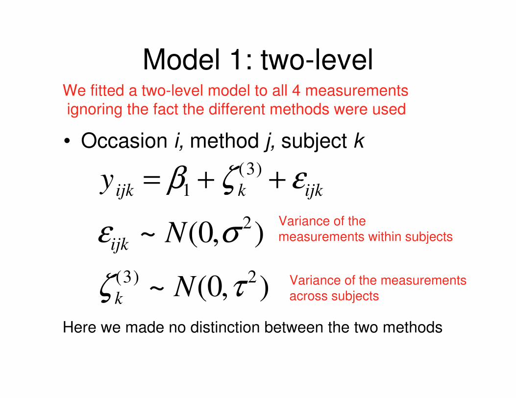
Model 1: two-level

• Occasion i, method j, subject k

y ijk = β1 + ζ k

(3) + εijk

εijk ~ N(0,σ 2)

ζ k

(3)~ N(0,τ 2

)

Here we made no distinction between the two methods

Variance of themeasurements within subjects

We fitted a two-level model to all 4 measurementsignoring the fact the different methods were used

Variance of the measurementsacross subjects

Model 2: two-level

• Occasion i, method j, subject k

y ijk = β1 + β2x j + ζ k

(3) + εijk

εijk ~ N(0,σ 2)

ζ k

(3)~ N(0,τ 2

)

Here we might add a binary variable for estimating themethods’ effect - this variable allows for a systematic

difference between the 2 methods

Intraclass correlation

coefficient

τ 2

τ 2 + σ 2=

109.22

109.22 + 23.8

2= 0.95

Correlation between the 4 repeated measures onthe same individual (the method used for the measurement

Is ignored)

The % of the total variance of the measurements

(within + between) that is explained by the variance of the measurementindividuals

Why we need three stage?occasion (i), method(j), individual (k)

• Both two-level variance component models assume that the four measurements using the two methods, were all mutually independent, conditional on the randomintercept (that is, they ignore the possibility that the measurements obtained with the same method might be more similar to each other than the measurements obtained with two different methods). In other words the measurements are “nested” within the “method”

• To see if this appears reasonable, we can plot all four measurements against subject id

Fig 7.2: Scatterplot of peak-respiratory flow measured by two methods versus

subject idmeasurements on the

same subjects are more similar

than measurements on different

subjects

For a given subject, the

measurements using

the same method

tend to resamble each

other more than

measurements

using the other method

The shift between the

measurements

taken from

the 2 methods

varies across

subjects

Why we need three-level models?

• As expected, measurements on the same subjects are more similar than measurements on different subjects. This between subject heterogeneity is modeled by the subject-level intercept .ς k

(3)

Why we need three-level

models• The figure suggests that for a given subject,

the measurements using the same method tend to be more similar to each other, violating the conditional independence assumption of model (1)

• The difference between methods is not due to some constant shift of the measurements using one method relative to the other, but due to shifts that vary between subjects, thus violating the assumption in model (2)

Model 3: three-level variance

component models

y ijk = β1 + ζ jk

(2) + ζ k

(3) + εijk

εijk ~ N(0,σ 2)

ζ jk

(2)~ N(0,τ 2

2)

ζ k

(3)~ N(0,τ 3

2)

Variance of the

measurements

across the two methods

for the same subject

Variance of the

measurements

across subjects

account for between-method

within-subject heterogeneity

Parameters interpretations

y ijk = β1 + ζ jk

(2) + ζ k

(3) + εijk

β1

β1 + ζ k

(3)

β1 + ζ jk

(2) + ζ k

(3)

Population average of all measurements (across

occasions, methods, and subjects)

Average of the measurements for subject k

(across occasions and methods)

Average of the measurements

for method j and for subject k (across

occasions)

Model 4: three-level variance

component models

y ijk = β1 + β2x j + ζ jk

(2) + ζ k

(3) + εijk

εijk ~ N(0,σ 2)

ζ jk

(2)~ N(0,τ 2

2)

ζ k

(3)~ N(0,τ 3

2)

Different types of intraclass correlation

ρ(subject) = cor(y ijk , y i' j 'k | x j ,x j ') =

=τ 3

2

τ 2

2 + τ 3

2 + σ 2

ρ(method,subject) = cor(y ijk ,y i' jk | x j ) =

=τ 2

2 + τ 3

2

τ 2

2 + τ 3

2 + σ 2

correlation between the 4

measurements within the subject

(same subject, different method, and

different occasion)

correlation between the

measurements obtained with the same

method and for the same subject (same

subject, same method, different occasions)

Intraclass correlations

• Note that cor(method,subject)> cor(subject). This makes sense since, as we saw in Figure 7.2, measurements using the same method are more similar than measurements usingdifferent methods for the same person.

Three-stage formulation

y ijk = η jk + β2x j + εijk

η jk = π k + ζ jk

(2)

π k = β1 + ζ jk

(3)

y ijk = β1 + β2x j + ζ jk

(2) + ζ jk

(3) + εijk

Stage 1

Stage 2

Stage 3

Random effect Fixed effect

Television school and family smoking

cessation project (TVSFP)

• The TVSFP is a study designed to determine the efficacy of a school-based smoking prevention program in conjunction with a television-basedprevention program, in terms of preventing smoking onset and increasing smoking cessation (Flay et al 1995)

TVSFP: outcome

• Outcome: a tobacco and health knowledge scale (THKS) assessing the student’s knowledge of tobacco and health

• Linear model for THKS post-intervention, with THKS pre-intervention as a covariate

TVSFP: study design

• 2x2 factorial design, with four intervention conditions determined by cross-classification of a school-based social resistant curriculum (CC: coded as 0 or 1) with a television-based program (TV, coded as 0 or 1)

• Randomization to one of the four intervention conditions was at the school level

• Intervention was delivered at the classroom level

• 1600 seventh-grades students from 135 classes in 28 schools in Los Angeles

Three-level model for the TVSFP

Yijk = β1 + β2 preTHKS + β3CC + β4TV + β5(CC × TV ) +

+bk

(3) + b jk

(2) + εijk

εijk ~ N(0,σ1

2)

b jk

(2)~ N(0,σ 2

2)

bk

(3)~ N(0,σ 3

2) Across schools

Within school, across classrooms

Within classroom, across students

i (student), j (classroom), k (school)

postTHKS

Intraclass correlation

coefficients

• Correlation among THKS scores for classmates (or children within the sameclass and same school) is 0.061

σ 3

2 + σ 2

2

σ 3

2 + σ 2

2 + σ1

2=

0.039 + 0.065

0.039 + 0.065 +1.602

Intraclass correlation

coefficients

• Correlation among THKS scores for children for different classrooms within the same school is 0.023

σ 3

2

σ 3

2 + σ 2

2 + σ1

2=

0.039

0.039 + 0.065 +1.602

Should we ignore the

intraclass correlation?• The intraclass correlation coefficients were

relatively small at both the school and at theclassroom levels.

• We might be tempted to think that the clustering of the data would not affect theintervention effects

• Such conclusion would be erroneous

• Although the intraclass correlations are small, they have substantial impact on the inferences

Linear model for the TVSFPwithout random effects

Yijk = β1 + β2 preTHKS + β3CC + β4TV + β5(CC × TV ) + εijk

εijk ~ N(0,σ1

2)

i (student), j (classroom), k (school)

postTHKS

This model ignores clustering in the data at a classroomand school levels. This is a standard linear regression model

and assumes that the responses are independent

Comparing results

• Model-based standard errors (assuming no clustering) and misleading small for the randomized intervention effects and lead to substantially different conclusions

• Bottom line: even a very modest intra-cluster correlation can have a discernable impact on the inferences