Mathematical Notes on SAMtools Algorithms

Heng Li

October 12, 2010

2

Chapter 1

Duplicate Rate

1.1 Amplicon duplicates

Let N be the number of distinct segments (or seeds) before the amplification and M be thetotal number of amplicons in the library. For seed i (i = 1, . . . , N), let ki be the numberof amplicons in the library and ki is drawn from Poinsson distribution Po(λ). When N issufficiently large, we have:

M =

N∑i=1

ki = N

∞∑k=0

kpk = Nλ

where pk = e−λλk/k!.At the sequencing step, we sample m amplicons from the library. On the condition that:

m�M (1.1)

we can regard this procedure as sampling with replacement. For seed i, let:

Xi =

{1 seed i has been sampled at least once0 otherwise

and then:

EXi = Pr{Xi = 1} = 1−(

1− kiM

)m' 1− e−kim/M

Let:

Z =

N∑i=1

Xi

be the number of seeds sampled from the library. The fraction of duplicates d is:

d = 1− E(Z)

m

' 1− N

m

∞∑k=0

(1− e−km/M

)pk

= 1− N

m+Ne−λ

m

∑k

1

k!

(λe−m/M

)k' 1− N

m

[1− e−λ · eλ(1−m/M)

]3

4 CHAPTER 1. DUPLICATE RATE

i.e.

d ' 1− N

m

(1− e−m/N

)(1.2)

irrelevant of λ. In addition, when m/N is sufficiently small:

d ≈ m

2N(1.3)

This deduction assumes that i) ki � M which should almost always stand; ii) m � Mwhich should largely stand because otherwise the fraction of duplicates will far more thanhalf given λ ∼ 1000 and iii) ki is drawn from a Poisson distribution.

The basic message is that to reduce PCR duplicates, we should either increase the originalpool of distinct molecules before amplification or reduce the number of reads sequenced fromthe library. Reducing PCR cycles, however, plays little role.

1.2 Alignment duplicates

For simplicity, we assume a read is as short as a single base pair. For m read pairs, definean indicator function:

Yij =

{1 if at least one read pair is mapped to (i, j)0 otherwise

Let {pk} be the distribution of insert size. Then:

EYij = Pr{Yij = 1} = 1−[1− pj−i

L− (j − i)

]m' 1− e−pj−i·m/[L−(j−i)]

where L is the length of the reference. The fraction of random coincidence is:

d′ = 1− 1

m

L∑i=1

L∑j=i

EYij

' 1− 1

m

L∑i=1

L∑j=i

(1− e−pj−i·m/(L−(j−i))

)= 1− 1

m

L−1∑k=0

(L− k)[1− e−pkm/(L−k)

]On the condition that L is sufficient large and:

m� L (1.4)

d′ ' m

2

L−1∑k=0

p2kL− k

(1.5)

We can calculate/approximate Equation 1.5 for two types of distributions. Firstly, if pkis evenly distributed between [k0, k0 + k1], d′ ' m

2k1L. Secondly, assume k is drawn from

N(µ, σ) with σ � 1:

pk =1√2πσ

∫ k+1

k

e−(x−µ)2

2σ2 dx ' 1√2πσ

e−(k−µ)2

2σ2

1.2. ALIGNMENT DUPLICATES 5

If p0 � 1, µ� L and L� 1:

d′ ' m

4πσ2

∫ 1

0

1

1− x· e−

(Lx−µ)2

σ2 dx

' m

4πσ2

∫ ∞−∞

e− (x−µ/L)2

(σ/L)2 dx

=m

4πσ2·√

2π ·√

2σ

L

=m

2√πσL

6 CHAPTER 1. DUPLICATE RATE

Chapter 2

Base Alignment Quality (BAQ)

Let the reference sequence be x = r1 . . . rL. We can use a profile HMM to simulate how aread y = ˆc1 . . . cl$ with quality z = q1 . . . ql is generated (or sequenced) from the reference,where ˆ stands for the start of the read sequence and $ for the end.

Figure 2.1: A profile HMM for generating sequence reads from a reference sequence, where L is thelength of the reference sequence, M states stand for alignment matches, I for alignment insertionsto the reference and D states for deletions.

The topology of the profile HMM is given in Fig 2.1. Let (M, I,D, S) = (0, 1, 2, 3). The

7

8 CHAPTER 2. BASE ALIGNMENT QUALITY (BAQ)

transition matrix between different types of states is

A = (aij)4×4 =

(1− 2α)(1− s) α(1− s) α(1− s) s(1− β)(1− s) β(1− s) 0 s

1− β 0 β 0(1− α)/L α/L 0 0

where α is the gap open probability, β is the gap extension probability and s = 1/(2l)with l being the average length of a read. As to emission probabilities, P (ci|Dk) = 1,P (ˆ|S) = P ($|S) = 1, P (ci|Ik) = 0.25 and

P (bi|Mk) = eki =

{1− 10−qi/10 if rk = bi10−qi/10/3 otherwise

The forward-backward algorithm1 is as follows:

fS(0) = 1

fMk(1) = ek1 · a30

fIk(1) = 0.25 · a31fMk

(i) = eki ·[a00fMk−1

(i− 1) + a10fIk−1(i− 1) + a20fDk−1

(i− 1)]

fIk(i) = 0.25 ·[a01fMk

(i− 1) + a11fIk(i− 1)]

fDk(i) = a02fMk−1(i) + a22fDk−1

(i)

fS(l + 1) =

L∑k=1

a03fMk(l) + a13fIk(l)

bS(l + 1) = 1

bMk(l) = a03

bIk(l) = a13

bMk(i) = ek+1,i+1a00bMk+1

(i+ 1) + a01bIk(i+ 1)/4 + a02bDk+1(i)

bIk(i) = ek+1,i+1a10bMk+1(i+ 1) + a11bIk(i+ 1)/4

bDk(i) = (1− δi1) ·[ek+1,i+1a20bMk+1

(i+ 1) + a22bDk+1(i)]

bS(0) =

L∑k=1

ek1a30bMk(1) + a31bIk(1)/4

and the likelihood of data is P (y) = fS(L+ 1) = bS(0)2. The posterior probability of a readbase ci being matching state k (M- or I-typed) is fk(i)bk(i)/P (y).

1We may adopt a banded forward-backward approximation to reduce the time complexity. We may alsonormalize fk(i) for each i to avoid floating point underflow.

2Evaluating if fS(L + 1) = bS(0) helps to check the correctness of the formulae and the implementation.

Chapter 3

Modeling Sequencing Errors

3.1 The revised MAQ model

3.1.1 General formulae

Firstly it is easy to prove that for any 0 ≤ βnk < 1 (0 ≤ k ≤ n),

n∑k=0

(1− βnk)

k−1∏l=0

βnl = 1−n∏k=0

βnk

where we regard that∏−1i=0 βni = 1. In particular, when ∃k ∈ [0, n] satisfies βnk = 0, we

have:n∑k=0

(1− βnk)

k−1∏i=0

βni = 1

If we further define:

αnk = (1− βnk)

k−1∏i=0

βni (3.1)

on the condition that some βnk = 0, we have:

n∑k=0

αnk = 1

βnk = 1− αnk

1−∑k−1i=0 αni

=1−

∑ki=0 αni

1−∑k−1i=0 αni

=

∑ni=k+1 αni∑ni=k αni

In the context of error modeling, if we define:

βnk ,

{Pr{at least k + 1 errors|at least k errors out of n bases} (k > 0)Pr{at least 1 error out of n bases} (k = 0)

we have βnn = 0, and

γnk ,k−1∏l=0

βnl = Pr{at least k errors out of n bases}

thenαnk = (1− βnk)γnk = Pr{exactly k errors in n bases}

9

10 CHAPTER 3. MODELING SEQUENCING ERRORS

3.1.2 Modeling sequencing errors

Given a uniform error rate ε and independent errors, let

αnk(ε) =

(n

k

)εk(1− ε)n−k

and

βnk(ε) =

∑ni=k+1 αni(ε)∑ni=k αni(ε)

we can calculate that the probability of seeing at least k errors is

γnk(ε) =

k−1∏l=0

βnk(ε)

When errors are dependent, the true βnk will be larger than βnk. A possible choice ofmodeling this is to let

βnk = βfknk

where 0 < fk ≤ 1 models the dependency for k-th error. The probability of seeing at least kerrors is thus

γnk(ε) =

k−1∏l=0

βflnl(ε)

For non-uniform errors ε1 ≤ ε2 ≤ · · · ≤ εn, we may approximate γnk(~ε) as

γnk(~ε) =

k−1∏l=0

βflnl(εl+1)

3.1.3 Practical calculation

We consider diploid samples only. Let g ∈ {0, 1, 2} be the number of reference alleles. Supposethere are k reference alleles whose base error rates are ε1 ≤ · · · ≤ εk, and there are n − kalternate alleles whose base error rates are ε′1 ≤ · · · ≤ ε′n−k. We calculate

P (D|0) = γnk(~ε) =

k−1∏l=0

βflnl(εl+1)

P (D|2) = γnk(~ε′) =

n−k−1∏l=0

βflnl(ε′l+1)

and

P (D|1) =1

2n

(n

k

)where fl = 0.97ηκl−1 + 0.03 with κl being the rank of base l among the same type of baseson the same strand, ordered by error rate. For sequencing data, error rates are usuallydiscretized. We may precompute βnk(ε) for sufficiently large n1 and all possible discretizedε. Calculating the likelihood of the data is trivial.

1SAMtools precomputes a table for n ≤ 255. Given higher coverage, it randomly samples 255 reads.

3.1. THE REVISED MAQ MODEL 11

3.1.4 The original MAQ model

The original MAQ models the likelihood of data by

αnk(ε) = (1− βfknk)

k−1∏i=0

βfini

instead of γnk(ε). For non-uniform errors,

αnk(~ε) = cnk(ε) ·k−1∏i=0

εfii+1

where

log ε =

∑k−1i=0 fi log εi+1∑k−1

i=0 fi

and

cnk(ε) ,[1− βfknk(ε)

] k−1∏i=0

[βni(ε)

ε

]fiThe major problem with the original MAQ model is that for ε close to 0.5 and large n,

the chance of seeing no errors may be so small that it is even smaller than the chance ofseeing all errors (i.e. αn0 < αnn). In this case, the model prefers seeing all errors, whichis counterintuitive. The revised model uses the accumulative probability γnk and does nothave this problem. For small ε and n, the original and the revised MAQ models seem to havesimilar performance.

12 CHAPTER 3. MODELING SEQUENCING ERRORS

Chapter 4

Modeling Multiple Individuals

4.1 Notations

Suppose there are N sites from n individuals with i-th individual having mi ploids. LetM =

∑imi be the total number of chromosomes. Let D = ( ~D1, . . . , ~DN )T be the data

matrix with vector ~Da = (Da1, . . . , Dan) representing the alignment data for each individual

at site a. Similary, let G = (~Ga, . . . , ~GN )T and ~Ga = (Ga1, . . . , Gan) be the true genotypes,where 0 ≤ Gai ≤ mi equals the number of reference alleles 1. Define

Xa = Xa(~Ga) ,∑i

Gai (4.1)

to be the number of reference alleles at site a and X = (X1, . . . , XN )T. Also define Φ =(φ0, . . . , φM ) as the allele frequency spectrum (AFS) with

∑k φk = 1.

For convenience, we may drop the position subscript a when it is unambiguous in thecontext that we are looking at one locus. Also define

P (Di|gi) , Pr{Di|Gi = gi} (4.2)

to be the likelihood of the data for individual i when the underlying genotype is known.P (Di|gi) is calculated in Section 4.4. And define

P (gi|φ) ,

(mi

gi

)φgi(1− φ)mi−gi (4.3)

to be the probability of a genotype under the Hardy-Weinberg equilibrium (HWE), when thesite allele frequency is φ.

4.2 Estimating AFS

4.2.1 The EM procedure

We aim to find Φ that maximizes P (D|Φ) by EM. Suppose at the t-th iteration the estimateis Φt. We have

log Pr{D,X = x|Φ} = log Pr{D|X = x}Pr{X = x|Φ} = C +∑a

log φxa

1If we take the ancestral sequence as the reference, the non-reference allele will be the derived allele.

13

14 CHAPTER 4. MODELING MULTIPLE INDIVIDUALS

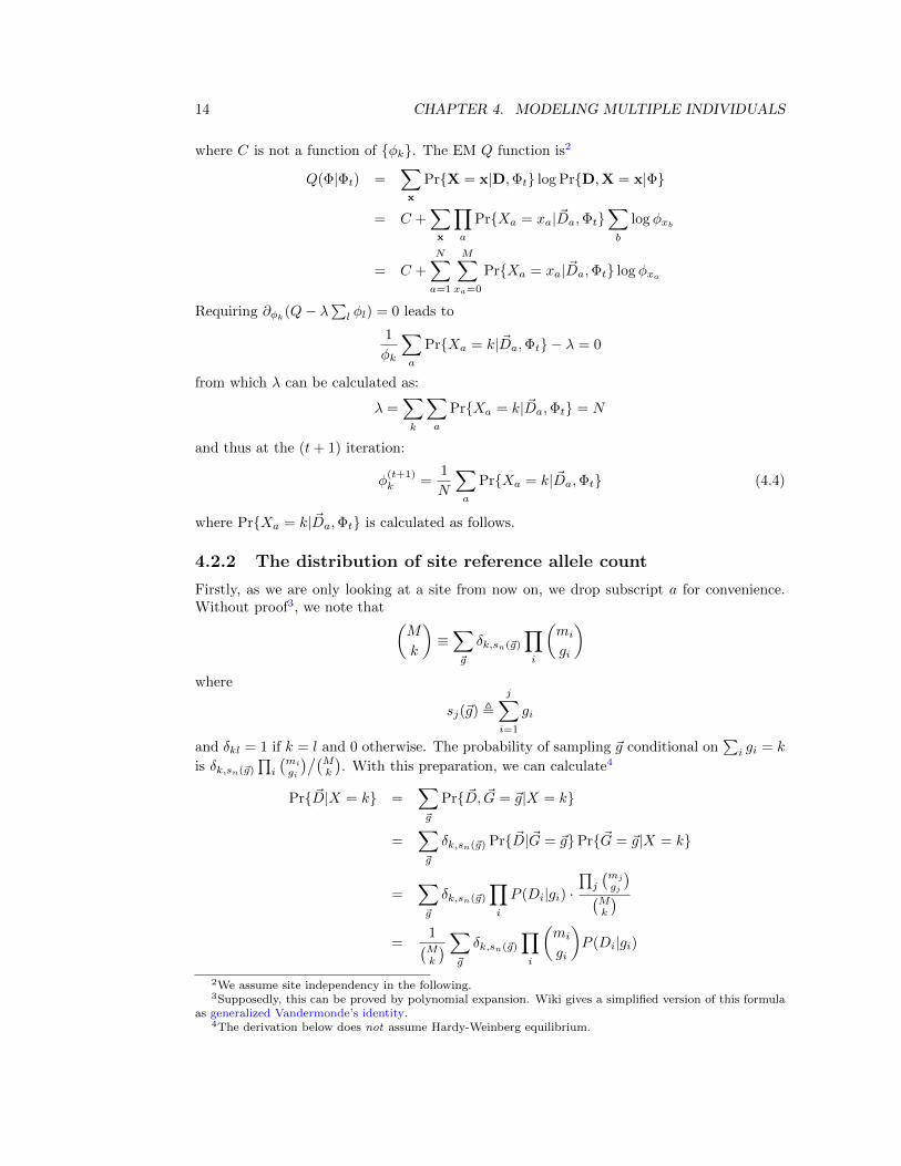
where C is not a function of {φk}. The EM Q function is2

Q(Φ|Φt) =∑x

Pr{X = x|D,Φt} log Pr{D,X = x|Φ}

= C +∑x

∏a

Pr{Xa = xa| ~Da,Φt}∑b

log φxb

= C +

N∑a=1

M∑xa=0

Pr{Xa = xa| ~Da,Φt} log φxa

Requiring ∂φk(Q− λ∑l φl) = 0 leads to

1

φk

∑a

Pr{Xa = k| ~Da,Φt} − λ = 0

from which λ can be calculated as:

λ =∑k

∑a

Pr{Xa = k| ~Da,Φt} = N

and thus at the (t+ 1) iteration:

φ(t+1)k =

1

N

∑a

Pr{Xa = k| ~Da,Φt} (4.4)

where Pr{Xa = k| ~Da,Φt} is calculated as follows.

4.2.2 The distribution of site reference allele count

Firstly, as we are only looking at a site from now on, we drop subscript a for convenience.Without proof3, we note that (

M

k

)≡∑~g

δk,sn(~g)∏i

(mi

gi

)where

sj(~g) ,j∑i=1

gi

and δkl = 1 if k = l and 0 otherwise. The probability of sampling ~g conditional on∑i gi = k

is δk,sn(~g)∏i

(migi

)/(Mk

). With this preparation, we can calculate4

Pr{ ~D|X = k} =∑~g

Pr{ ~D, ~G = ~g|X = k}

=∑~g

δk,sn(~g) Pr{ ~D|~G = ~g}Pr{~G = ~g|X = k}

=∑~g

δk,sn(~g)∏i

P (Di|gi) ·∏j

(mjgj

)(Mk

)=

1(Mk

) ∑~g

δk,sn(~g)∏i

(mi

gi

)P (Di|gi)

2We assume site independency in the following.3Supposedly, this can be proved by polynomial expansion. Wiki gives a simplified version of this formula

as generalized Vandermonde’s identity.4The derivation below does not assume Hardy-Weinberg equilibrium.

4.2. ESTIMATING AFS 15

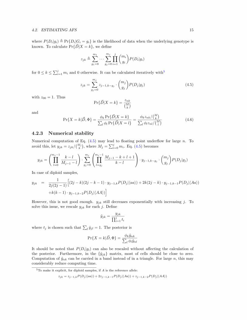
where P (Di|gi) , Pr{Di|Gi = gi} is the likelihood of data when the underlying genotype is

known. To calculate Pr{ ~D|X = k}, we define

zjk ,m1∑g1=0

· · ·mj∑gj=0

j∏i=1

(mi

gi

)P (Di|gi)

for 0 ≤ k ≤∑ji=1mi and 0 otherwise. It can be calculated iteratively with5

zjk =

mj∑gj=0

zj−1,k−gj ·(mj

gj

)P (Dj |gj) (4.5)

with z00 = 1. Thus

Pr{ ~D|X = k} =znk(Mk

)and

Pr{X = k| ~D,Φ} =φk Pr{ ~D|X = k}∑l φl Pr{ ~D|X = l}

=φkznk/

(Mk

)∑l φlznl/

(Ml

) (4.6)

4.2.3 Numerical stability

Numerical computation of Eq. (4.5) may lead to floating point underflow for large n. To

avoid this, let yjk = zjk/(Mj

k

), where Mj =

∑ji=0mi. Eq. (4.5) becomes

yjk =

(mj−1∏l=0

k − lMj−1 − l

)·mj∑gj=0

mj−1∏l=gj

Mj−1 − k + l + 1

k − l

· yj−1,k−gj · (mj

gj

)P (Dj |gj)

In case of diploid samples,

yjk =1

2j(2j − 1)

[(2j − k)(2j − k − 1) · yj−1,kP (Dj |〈aa〉) + 2k(2j − k) · yj−1,k−1P (Dj |〈Aa〉)

+k(k − 1) · yj−1,k−2P (Dj |〈AA〉)]

However, this is not good enough. yjk still decreases exponentially with increasing j. Tosolve this issue, we rescale yjk for each j. Define

yjk =yjk∏ji=1 ti

where tj is chosen such that∑l yjl = 1. The posterior is

Pr{X = k| ~D,Φ} =φkynk∑l φlynl

It should be noted that P (Di|gi) can also be rescaled without affecting the calculation ofthe posterior. Furthermore, in the {yjk} matrix, most of cells should be close to zero.Computation of ynk can be carried in a band instead of in a triangle. For large n, this mayconsiderably reduce computing time.

5To make it explicit, for diploid samples, if A is the reference allele:

zjk = zj−1,kP (Dj |〈aa〉) + 2zj−1,k−1P (Dj |〈Aa〉) + zj−1,k−2P (Dj |〈AA〉)

16 CHAPTER 4. MODELING MULTIPLE INDIVIDUALS

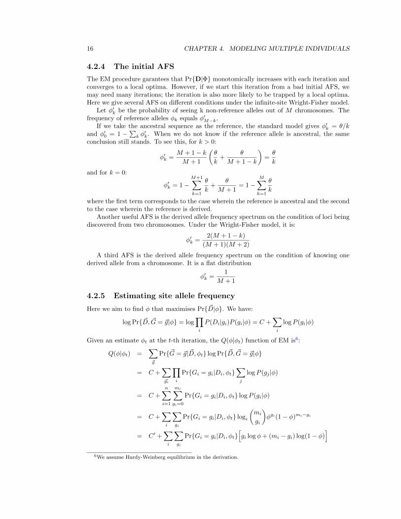
4.2.4 The initial AFS

The EM procedure garantees that Pr{D|Φ} monotomically increases with each iteration andconverges to a local optima. However, if we start this iteration from a bad initial AFS, wemay need many iterations; the iteration is also more likely to be trapped by a local optima.Here we give several AFS on different conditions under the infinite-site Wright-Fisher model.

Let φ′k be the probability of seeing k non-reference alleles out of M chromosomes. Thefrequency of reference alleles φk equals φ′M−k.

If we take the ancestral sequence as the reference, the standard model gives φ′k = θ/kand φ′0 = 1 −

∑k φ′k. When we do not know if the reference allele is ancestral, the same

conclusion still stands. To see this, for k > 0:

φ′k =M + 1− kM + 1

(θ

k+

θ

M + 1− k

)=θ

k

and for k = 0:

φ′k = 1−M+1∑k=1

θ

k+

θ

M + 1= 1−

M∑k=1

θ

k

where the first term corresponds to the case wherein the reference is ancestral and the secondto the case wherein the reference is derived.

Another useful AFS is the derived allele frequency spectrum on the condition of loci beingdiscovered from two chromosomes. Under the Wright-Fisher model, it is:

φ′k =2(M + 1− k)

(M + 1)(M + 2)

A third AFS is the derived allele frequency spectrum on the condition of knowing onederived allele from a chromosome. It is a flat distribution

φ′k =1

M + 1

4.2.5 Estimating site allele frequency

Here we aim to find φ that maximises Pr{ ~D|φ}. We have:

log Pr{ ~D, ~G = ~g|φ} = log∏i

P (Di|gi)P (gi|φ) = C +∑i

logP (gi|φ)

Given an estimate φt at the t-th iteration, the Q(φ|φt) function of EM is6:

Q(φ|φt) =∑~g

Pr{~G = ~g| ~D, φt} log Pr{ ~D, ~G = ~g|φ}

= C +∑~gi

∏i

Pr{Gi = gi|Di, φt}∑j

logP (gj |φ)

= C +

n∑i=1

mi∑gi=0

Pr{Gi = gi|Di, φt} logP (gi|φ)

= C +∑i

∑gi

Pr{Gi = gi|Di, φt} logi

(mi

gi

)φgi(1− φ)mi−gi

= C ′ +∑i

∑gi

Pr{Gi = gi|Di, φt}[gi log φ+ (mi − gi) log(1− φ)

]6We assume Hardy-Weinberg equilibrium in the derivation.

4.2. ESTIMATING AFS 17

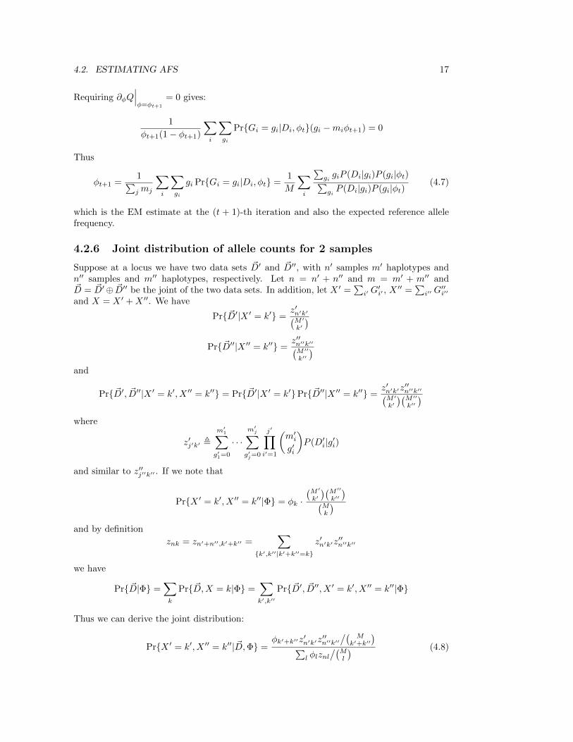
Requiring ∂φQ∣∣∣φ=φt+1

= 0 gives:

1

φt+1(1− φt+1)

∑i

∑gi

Pr{Gi = gi|Di, φt}(gi −miφt+1) = 0

Thus

φt+1 =1∑jmj

∑i

∑gi

gi Pr{Gi = gi|Di, φt} =1

M

∑i

∑gigiP (Di|gi)P (gi|φt)∑giP (Di|gi)P (gi|φt)

(4.7)

which is the EM estimate at the (t + 1)-th iteration and also the expected reference allelefrequency.

4.2.6 Joint distribution of allele counts for 2 samples

Suppose at a locus we have two data sets ~D′ and ~D′′, with n′ samples m′ haplotypes andn′′ samples and m′′ haplotypes, respectively. Let n = n′ + n′′ and m = m′ + m′′ and~D = ~D′⊕ ~D′′ be the joint of the two data sets. In addition, let X ′ =

∑i′ G′i′ , X

′′ =∑i′′ G

′′i′′

and X = X ′ +X ′′. We have

Pr{ ~D′|X ′ = k′} =z′n′k′(M ′

k′

)Pr{ ~D′′|X ′′ = k′′} =

z′′n′′k′′(M ′′

k′′

)and

Pr{ ~D′, ~D′′|X ′ = k′, X ′′ = k′′} = Pr{ ~D′|X ′ = k′}Pr{ ~D′′|X ′′ = k′′} =z′n′k′z

′′n′′k′′(

M ′

k′

)(M ′′

k′′

)where

z′j′k′ ,m′1∑g′1=0

· · ·m′j∑g′j=0

j′∏i′=1

(m′ig′i

)P (D′i|g′i)

and similar to z′′j′′k′′ . If we note that

Pr{X ′ = k′, X ′′ = k′′|Φ} = φk ·(M ′

k′

)(M ′′

k′′

)(Mk

)and by definition

znk = zn′+n′′,k′+k′′ =∑

{k′,k′′|k′+k′′=k}

z′n′k′z′′n′′k′′

we have

Pr{ ~D|Φ} =∑k

Pr{ ~D,X = k|Φ} =∑k′,k′′

Pr{ ~D′, ~D′′, X ′ = k′, X ′′ = k′′|Φ}

Thus we can derive the joint distribution:

Pr{X ′ = k′, X ′′ = k′′| ~D,Φ} =φk′+k′′z

′n′k′z

′′n′′k′′

/(M

k′+k′′

)∑l φlznl

/(Ml

) (4.8)

18 CHAPTER 4. MODELING MULTIPLE INDIVIDUALS

If we let yjk = zjk/(Mj

k

)as in Section 4.2.3,

Pr{X ′ = k′, X ′′ = k′′| ~D,Φ} =φk′+k′′y

′n′k′y

′′n′′k′′∑

l φlynl·(M ′

k′

)(M ′′

k′′

)(M ′+M ′′

k′+k′′

)This derivation can be extended to arbitrary number of data sets.

4.2.7 Estimating 2-locus haplotype frequency

In this section, we only consider diploid samples (i.e. m1 = · · · = mn = 2). Let D = ( ~D, ~D′)

be the data at two loci, respectively; and Hi and H†i be the two underlying haplotypes forindividual i with Hi ∈ {0, 1, 2, 3} representing one of the four possible haplotypes at the 2

loci. We write H =−−−−−→(Hi, H

†i ) as a haplotype configuration of the samples. Define

Ghk = bh/2c+ bk/2c

G′hk = (h mod 2) + (k mod 2)

which calculate the genotype of each locus, respectively.

Q(~φ|~φ(t)) =∑h

P (H = h|D, ~φ(t)) log Pr{D,H = h|~φ}

= C +∑h

∏i

Pr{Hi = hi, H†i = h†i |D, ~φ

(t)}∑j

logP (hj , h†j |~φ)

= C +∑i

∑hi

∑h†i

Pr{Hi = hi, H†i = h†i |D, ~φ

(t)}∑j

log(φhiφh†i)

Solving ∂φkQ− λ = 0 gives

φk =1

2n

∑i

∑h

(Pr{Hi = h,H†i = k|D, ~φ(t)}+ Pr{Hi = k,H†i = h|D, ~φ(t)}

)=

φ(t)k

2n

n∑i=1

∑h φ

(t)h

[P (Di|Ghk)P (D′i|G′hk) + P (Di|Gkh)P (D′i|G′kh)

]∑k′,h φ

(t)k′ φ

(t)h P (Di|Ghk′)P (D′i|G′hk′)

4.3 An alternative model

In Section 4.2, φk in Φ = {φk} is interpreted as the probability of seeing exactly k allelesfrom M chromosomes. Under this model, the prior of a genotype configuration is

Pr{~G = ~g|Φ} = φsn(~g)

∏i

(migi

)(M

sn(~g)

)and the posterior is

Pr{~G = ~g| ~D,Φ} =φsn(~g)

Pr{ ~D|Φ}·∏i

(migi

)P (Di|gi)(M

sn(~g)

)Suppose we want to calculate the expectation of

∑i fi(gi), we can∑

i

∑~g

fi(gi) Pr{~G = ~g| ~D,Φ} =1

Pr{ ~D|Φ}

∑i

∑k

φk(Mk

) ∑~g

δk,sn(~g)fi(gi)∏j

(mj

gj

)P (Dj |gj)

4.3. AN ALTERNATIVE MODEL 19

Due to the presence of δk,sn(~g), we are unable to reduce the formula to a simpler form. Al-though we can take a similar strategy in Section 4.2 to calculate

∑k

∑~g, which is O(n2),

another sum∑i will bring this calculation to O(n3). Even calculating the marginal prob-

ability Pr{Gi = gi| ~D,Φ} requires this time complexity. All the difficulty comes from thatindividuals are correlated conditional on {X = k}.

An alternative model is to interpret the AFS as the discretized AFS of the populationrather than for the observed individuals. We define the population AFS discretized on Mchromosomes as Φ′ = {φ′k}. Under this model,

Pr{~G = ~g|Φ′} =∑k

φk∏i

P (gi|k/M)

Pr{~G = ~g, ~D|Φ′} =∑k

φk∏i

P (Di|gi)P (gi|k/M)

Pr{ ~D|Φ′} =∑~g

Pr{~G = ~g, ~D|Φ′} =

M∑k=0

φ′k

n∏i=1

mi∑gi=0

P (Di|gi)P (gi|k/M)

and ∑i

∑~g

fi(gi) Pr{~G = ~g| ~D,Φ′} (4.9)

=1

Pr{ ~D|Φ′}

∑i

∑~g

fi(gi)∑k

φ′k∏j

P (Dj |gj)P (gj |k/M)

=1

Pr{ ~D|Φ′}

∑k

φ′k∑i

fi(gi)P (Di|gi)P (gi|k/M)∏j 6=i

∑gj

P (Dj |gj)P (gj |k/M)

=1

Pr{ ~D|Φ′}

∑k

φ′k

[∏i

∑gi

P (Di|gi)P (gi|k/M)

]·

[∑i

∑gifi(gi)P (Di|gi)P (gi|k/M)∑giP (Di|gi)P (gi|k/M)

]

The time complexity of this calculation is O(n2). Consider that if fi(gi) = gi, X =∑i fi(Gi).

We can easily calculate E(X| ~D,Φ′) with the formula above.

4.3.1 Posterior distribution of the allele count

Under the alternative model, we can also derive the posterior distribution of X, Pr{X =

k| ~D,Φ′} as follows.

Pr{X = k|Φ′} =

(M

k

) M∑l=0

φ′l

(l

M

)k (1− l

M

)M−kThen

Pr{ ~D,X = k|Φ′} = znk

M∑l=0

φ′l

(l

M

)k (1− l

M

)M−k(4.10)

In fact, we also have an alternative way to derive this Pr{ ~D,X = k|Φ′}. Let φ′ be the

20 CHAPTER 4. MODELING MULTIPLE INDIVIDUALS

true site allele frequency in the population. Assuming HWE, we have

Pr{X = k, ~D|φ′} =∑~g

δk,sn(~g) Pr{ ~D|~G = ~g}Pr{~G = ~g|φ′} (4.11)

=∑~g

δk,sn(~g)∏i

P (D|gi)(mi

gi

)φ′gi(1− φ′)mi−gi

= φ′k(1− φ′)M−k∑~g

δk,sn(~g)∏i

(mi

gi

)P (Di|gi)

= φ′k(1− φ′)M−kznk

Summing over the AFS gives

Pr{ ~D,X = k|Φ′} =∑l

φ′l Pr{X = k, ~D|φ′ = l/M}

which is exactly Eq. (4.10). It is worth noting that E(X| ~D,Φ′) calculated by Eq. (4.11) isidentical to the one calculated by Eq. (4.9), which has been numerically confirmed.

In practical calculation, the alternative model has very similar performance to the methodin Section 4.2 in one iteration. However, in proving EM, we require Pr{X = k|Φ} = φk,which does not stand any more in the alternative interpretation. Iterating Eq. (4.10) maynot monotonically increase the likelihood function. Even if this was also another differentEM procedure, we have not proved it yet. Yi et al. (2010) essentially calculates Eq. (4.11) forφ′ estimated from data without summing over the AFS. Probably this method also deliverssimilar results, but it is not theoretically sound and may not be iterated, either.

4.4 Likelihood of data given genotype

Given a site covered by k reads from an m-ploid individual, the sequencing data is:

D = (b1, . . . , bk) = (1, . . . , 1︸ ︷︷ ︸l

, 0, . . . , 0︸ ︷︷ ︸k−l

)

where 1 stands for a reference allele and 0 otherwise. The j-th base is associated with errorrate εj , which is the larger error rate between sequencing and alignment errors. We have

P (D|0) =

l∏j=1

εj

k∏j=l+1

(1− εj) =

1−k∑

j=l+1

εj + o(ε2)

l∏j=1

εj (4.12)

P (D|m) =

1−l∑

j=1

εj + o(ε2)

k∏j=l+1

εj (4.13)

4.5. MULTI-SAMPLE SNP CALLING AND GENOTYPING 21

For 0 < g < m:

P (D|g) =

1∑a1=0

· · ·1∑

ak=0

Pr{D|B1 = a1, . . . , Bk = ak}Pr{B1 = a1, . . . , Bk = ak|g}(4.14)

=∑~a

( gm

)∑j aj(

1− g

m

)k−∑j aj ·∏j

pj(aj)

=(

1− g

m

)k∏j

1∑a=0

pj(a)

(g

m− g

)a

=(

1− g

m

)k l∏j=1

(εj +

g

m− g(1− εj)

) k∏j=l+1

(1− εj +

εjg

m− g

)

=(

1− g

m

)k(

g

m− g

)l+

(1− g

m− g

) l∑j=1

εj −k∑

j=l+1

εj

+ o(ε2)

In the bracket, the first term explains the deviation between l/k and g/m by imperfectsampling, while the second term explains the deviation by sequencing errors. The secondterm can be ignored when k is small but may play a major role when k is large. In particular,for m = 2, P (D|1) = 2−k, independent of sequencing errors.

In case of dependent errors, we may replace:

ε1 < ε2 < · · · < εl

withε′j = εα

j−1

j

where parameter α ∈ [0, 1] addresses the error dependency.

4.5 Multi-sample SNP calling and genotyping

The probability of the site being polymorphic is Pr{X = 0| ~D,Φ}. For individual i, we mayestimate the genotype gi as:

gi = argmaxgi

Pr{Gi = gi|Di, φE} = argmaxgi

P (Di|gi)P (gi|φE)∑hiP (Di|hi)P (hi|φE)

whereφE = E(X| ~D,Φ)/M

This estimate of genotypes may not necessarily maximize the posterior probability P (~g| ~D),but it should be good enough in practice. However, it should be noted that

∑i gi is usually

a bad estimator of site allele frequency. The max-likelihood estimator by Eq. (4.7) is muchbetter.