econstorMake Your Publications Visible.

A Service of

zbwLeibniz-InformationszentrumWirtschaftLeibniz Information Centrefor Economics

Barlevy, Gadi; Neal, Derek

Working Paper

Pay for percentile

Working Paper, No. 2009-09

Provided in Cooperation with:Federal Reserve Bank of Chicago

Suggested Citation: Barlevy, Gadi; Neal, Derek (2009) : Pay for percentile, Working Paper, No.2009-09, Federal Reserve Bank of Chicago, Chicago, IL

This Version is available at:http://hdl.handle.net/10419/70486

Standard-Nutzungsbedingungen:

Die Dokumente auf EconStor dürfen zu eigenen wissenschaftlichenZwecken und zum Privatgebrauch gespeichert und kopiert werden.

Sie dürfen die Dokumente nicht für öffentliche oder kommerzielleZwecke vervielfältigen, öffentlich ausstellen, öffentlich zugänglichmachen, vertreiben oder anderweitig nutzen.

Sofern die Verfasser die Dokumente unter Open-Content-Lizenzen(insbesondere CC-Lizenzen) zur Verfügung gestellt haben sollten,gelten abweichend von diesen Nutzungsbedingungen die in der dortgenannten Lizenz gewährten Nutzungsrechte.

Terms of use:

Documents in EconStor may be saved and copied for yourpersonal and scholarly purposes.

You are not to copy documents for public or commercialpurposes, to exhibit the documents publicly, to make thempublicly available on the internet, or to distribute or otherwiseuse the documents in public.

If the documents have been made available under an OpenContent Licence (especially Creative Commons Licences), youmay exercise further usage rights as specified in the indicatedlicence.

www.econstor.eu

F

eder

al R

eser

ve B

ank

of C

hica

go

Pay for Percentile Gadi Barlevy and Derek Neal

WP 2009-09

PAY FOR PERCENTILE

GADI BARLEVY

FEDERAL RESERVE BANK OF CHICAGO

DEREK NEAL

UNIVERSITY OF CHICAGO AND NBER

Date: August, 2009.We thank Fernando Alvarez, Julian Betts, Ann Bartel, John Kennan, Kevin Lang, Roger Myerson, KevinMurphy, Phil Reny, Doug Staiger, Chris Taber, and Azeem Shaikh for helpful comments and discussions.Neal thanks Lindy and Michael Keiser for research support through a gift to the University of Chicago’sCommittee on Education. Neal also thanks the Searle Freedom Trust. Our views need not reflect those ofthe Federal Reserve Bank of Chicago or the Federal Reserve System.

ABSTRACT

We propose an incentive pay scheme for educators that links educator compensation tothe ranks of their students within appropriately defined comparison sets, and we show thatunder certain conditions our scheme induces teachers to allocate socially optimal levels ofeffort to all students. Because this scheme employs only ordinal information, our schemeallows education authorities to employ completely new assessments at each testing datewithout ever having to equate various assessment forms. This approach removes incentivesfor teachers to teach to a particular assessment form and eliminates opportunities to influ-ence reward pay by corrupting the equating process or the scales used to report assessmentresults. Our system links compensation to the outcomes of properly seeded contests ratherthan cardinal measures of achievement growth. Thus, education authorities can employ ourincentive scheme for educators while employing a separate system for measuring growth instudent achievement that involves no stakes for educators. This approach does not createdirect incentives for educators to take actions that contaminate the measurement of studentprogress.

1. Introduction

In modern economies, most wealth is held in the form of human capital, and publiclyfunded schools play a key role in creating this wealth. Thus, reform proposals that seek toenhance the efficiency of schools are an omnipresent feature of debates concerning publicpolicy and societal welfare. In recent decades, education policy makers have increasinglydesigned these reform efforts around measures of school output such as test scores ratherthan measures of school inputs such as computer labs or student-teacher ratios. Althoughscholars and policy makers still debate the benefits of smaller classes, improved teacherpreparation, or improved school facilities, few are willing to measure school quality usingonly measures of school inputs. During the 1990s many states adopted accountabilitysystems that dictated sanctions and remediation for schools based on how their studentsperformed on standardized assessments. In 2001, the No Child Left Behind Act (NCLB)mandated that all states adopt such systems or risk losing federal funds, and more recently,several states and large districts have introduced incentive pay systems that link the salariesof individual teachers to the performance of their students.

A large empirical literature examines the effects of assessment based incentive systems,but to date, no literature formally explores the optimal design of these systems. Our paperis a first step toward filling this void. We pose the provision of teacher incentives as amechanism design problem. In our setting, an education authority possesses two sets oftest scores for a population of students. The first set of scores provides information aboutstudent achievement at the beginning (fall) of a school year. The second set providesinformation about the achievement of the same population of students at the end (spring)of the school year. Taken together, these test scores provide information concerning theeffort that teachers invested in their students.

We begin by noting that if the authority knows the mapping between the test score scaleand the expected value of student skill, the authority can implement efficient effort using anincentive scheme that pays teachers for the skills that their efforts helped create. Some willcontend that social scientists have no idea how to construct such a mapping and thereforeargue that such performance pay systems are infeasible.1 However, even if policy makersare able to discover the mapping between a particular test score scale and the value of

1See Balou (2009) for more on difficulties of interpreting psychometric scales. Cawley et al (1999) addressthe task of using psychometric scales in value-added pay for performance schemes. Cunha and Heckman(2008) describe methods for anchoring psychometric scales to adult outcomes. Their methods cannot beapplied to new incentive systems involving new assessments because data on the adult outcomes of testtakers cannot be collected before a given generation of students ages into adulthood.

student skill, the authority will find it challenging to maintain this mapping across a seriesof assessments.

It is well established that scores on a particular assessment become inflated when teacherscan coach students on the format or content of specifc items. In order to deter this type ofcoaching, education authorities typically employ a series of assessments that differ in termsof specific item content and form. But, in order to map results from each assessment into acommon scale, the authority must equate the various assessment forms, and proper equatingoften requires common items that link the various forms.2 If designers limit the numberof common items, they advance the goal of preventing teachers from coaching studentsfor specific questions or question formats, but they hinder the goal of properly equatingand thus properly scaling the various assessment forms. In addition, because equating isa complex task and proper equating is difficult to verify, the equating process itself is anobvious target for corruption.3

Given these observations, we turn our attention to mechanisms that require authoritiesto make incentive payments based only on the ordinal information contained in assessmentresults, without any knowledge of how the fall and spring assessments are scaled. Becausesuch systems involve no attempt to equate various assessment forms, they can includecompletely new assessment forms at each point in time and thus eliminate incentives tocoach students regarding any particular form of an assessment.

We describe a system called “pay for percentile,” that works as follows. For each studentin a school system, first form a comparison set of students against which the student will becompared. Assumptions concerning the nature of instruction dictate exactly how to definethis comparison set, but the general idea is to form a set that contains all other studentsin the system who begin the school year at the same level of baseline achievement in acomparable classroom setting. At the end of the year, give a cumulative assessment to allstudents. Then, assign each student a percentile score based on his end of year rank amongthe students in his comparison set. For each teacher, sum these within-peer percentile scoresover all the students she teaches and denote this sum as a percentile performance index.

2A common alternative approach involves randomly assigning one of several alternate forms to studentsin a large population, and then developing equating procedures based on the fact that the distribution ofachievement in the population receiving each form should be constant. This approach also invites coachingbecause, at the beginning of the second year of any test based incentive program, educators know that eachof their students will receive one of the forms used in the previous period.3A significant literature on state level proficiency rates under NCLB suggests that political pressures havecompromised the meaning of proficiency cutoff scores in numerous states. States can inflate their proficiencyrates by making exams easier while holding scoring procedures constant or by introducing a completely newassessment and then producing a crosswalk between the old and new assessment scale that effectively lowersthe proficiency threshold. See Cronin et al (2007)

2

Then, pay each teacher a common base salary plus a bonus that is proportional to herpercentile performance index. We demonstrate that this system can elicit efficient effortfrom all teachers in all classrooms to all students.

The linear relationship between bonus pay and our index does not imply that percentileunits are a natural or desirable scale for human capital. Rather, percentiles within com-parison sets tell us what fraction of head-to-head contests teachers win when competingagainst other teachers who educate similar students. For example, a student with a within-comparison set percentile score of .5 performed as well or better than half of his peers.Thus, in our scheme, his teacher gets credit for beating half of the teachers who taughtsimilar students. A linear relationship between total bonus pay and the fraction of contestswon works because all of the contests share an important symmetry. Each pits a studentagainst a peer who has the same expected spring achievement when both receive the sameinstruction and tutoring from their teachers.

The scheme we propose extends the work of Lazear and Rosen (1981). They demonstratethat tournaments can elicit efficient effort from workers when firms are only able to rank theperformance of their workers. In their model, workers make one effort choice and competein one contest. In our model, teachers make multiple effort choices, and these choices maysimultaneously affect the outcomes of many contests, but we still find that a common prizefor winning each tournament can induce efficient effort. Further, we show that pay forpercentile can elicit efficient effort in the presence of heterogeneous gains from instruction,instructional spillovers, and direct peer effects among students in the same classroom. Weare able to examine these issues because our model examines contestants who compete inmultiple contests simltaneously.

Within our framework, it is natural to think of teachers as workers who perform complexjobs that require multiple tasks because each teacher devotes effort to general classroominstruction as well as one-on-one tutoring for each student. Our results offer new insightfor the design of incentives in this setting. Imagine any setting where many workers occupythe same job, and this job requires the execution of multiple tasks. If employers can forman ordinal ranking of worker performance on each task that defines the job, these rankingsimply a set of winning percentages for each worker that describe the fraction of workersthat perform each task less well than she does. Our main results shows that employers canform an optimal bonus scheme by forming a weighted sum of these winning percentages.

Many engaged in current education policy debates implicitly argue that proper equatingof different exam forms is fundamental to sound education policy because education author-ities must be able to document the evolution of the distribution of student achievement over

3

time. But, we argue that education authorities should treat the provision of incentives andthe documenting of student progress as separate tasks. Equating studies are not necessaryfor incentive provision, and the equating process is more likely to be corrupted when highstakes are attached to the exams in question.

Some may worry that our system also provides incentives for teachers to engage in activ-ities that inflate assessment results relative to student subject mastery, and it is true thatour system does not address the various forms of outright cheating that test-based incentivesystems often invite. However, our goal is to design a system that specifically eliminatesincentives for teachers to coach students concerning the answers to particular questions orstrategies for taking tests rather than teaching students to master a given curriculum. Fur-ther, it is important to note that we are proposing a mechanism designed to induce teachersto teach a given curriculum. We do not address the often voiced concern that potentiallyimportant dimensions of student skill, e.g. creativity and curiosity, may not be included incurricular definitions.4

2. Basic Model

Here, we describe our basic model and derive optimal teacher effort for our setting. As-sume there are J classrooms, indexed by j ∈ {1, 2...J}. Each classroom has one teacher,so j also indexes teachers. We assume all teachers are equally effective in fostering thecreation of human capital among their students, and all teachers face the same costs of pro-viding effective instruction. This restriction allows us to focus on the task of eliciting effortfrom teachers, but it does not allow us to address other issues that arise in settings withheterogeneous teachers, such as how teachers should be screened for hiring and retentionand who should be assigned to teach which students.

Each classroom has N students, indexed by i ∈ {1, 2...N}. Let aij denote the initialhuman capital of the i-th student in the j-th class. Students within each class are orderedfrom least to most able, i.e.

a1j ≤ a2j ≤ · · · ≤ aNjWe assume all J classes are identical, i.e. aij = ai for all j ∈ {1, 2...J}. However, this

does not mean that our analysis only applies to an environment where all classes sharea common baseline achievement distribution. The task of determining efficient effort fora school system that contains heterogeneous classes can be accomplished by determining

4In their well-known paper on multi-tasking, Holmstrom and Milgrom (1991) highlight this concern as animportant cost associated with implementing assessment based incentive systems for teachers.

4

efficient effort for each classroom type. Thus, the planner may solve the allocation problemfor the system by solving the problem we analyze for each baseline achievement distributionthat exists in one or more classes.5

Teachers can undertake two types of efforts to help students acquire additional humancapital. They can tutor individual students or teach the class as a whole. Let eij denote theeffort teacher j spends on individual instruction of student i, and tj denote the effort shespends on classroom teaching. We assume the following educational production function:

(2.1) a′ij = g(ai) + tj + αeij + εij

The human capital of a student at the end of the period, denoted a′ij , depends on his initialskill level ai, the efforts of his teacher eij and tj , and a shock εij that does not dependon teacher effort, e.g. random disruptions to the student’s life at home. For now, weassume the production of human capital is separable between the student’s initial humancapital and all other factors and is linear in teacher efforts. Thus, the tutoring instructionis student-specific, and any effort spent on teaching student i will not directly affect anystudent i′ 6= i. Classroom teaching benefits all students in the class. Examples includetasks like lecturing or planning assignments. Here, g(·) is an increasing function and α > 0measures the relative productivity of classroom teaching versus individual instruction, andthe productivities of both tutoring effort and classroom instruction are not a functionof a student’s baseline achievement or the baseline achievement of his classmates. Thisspecification provides a useful starting point because it allows us to present our key resultswithin an analytically simple framework. In section 6, we consider more general productiontechnologies that permit not only heterogeneous gains from instruction among studentsbut also direct peer effects and instructional spillovers within a classroom. The results wederive concerning the efficiency of linking a teacher’s bonus pay to her winning percentagein contests against other teachers remain given all of these different generalizations to theproduction technology, but different technology assumptions may dictate different rules forseeding these contests.

The shocks εij are mean zero, pairwise independent for any pair (i, j), and identicallydistributed according to a common, continuous distribution F (x) ≡ Pr(εij ≤ x).

5We assume the planner takes the composition of each class as given. One could imagine a more generalproblem where the planner chooses the composition of classrooms and the effort vector for each classroom.However, given the optimal composition of classrooms, the planner still needs to choose the optimal levelsof effort in each class. We focus on this second step because we are analyzing the provision of incentivesfor educators taking as given the sorting of students among schools and classrooms.

5

Let Xj denote teacher j’s expected income. Then her utility is

(2.2) Uj = Xj − C(e1j , ..., eNj , tj)

where C(·) denotes the teacher’s cost of effort. We assume C(·) is increasing in all ofits arguments and is strictly convex. We further assume it is symmetric with respect toindividual tutoring efforts, i.e. let ej be any vector of tutoring efforts (e1j , ..., eNj) forteacher j, and let e′j be any permutation of ej , then

C(ej , , tj) = C(e′j , tj)

We also impose the usual boundary conditions on marginal costs. The lower and upperlimits of the marginal costs with respect to each dimension of effort are 0 and∞ respectively.These conditions ensure the optimal plan will be interior. Although we do not make itexplicit, C(·) also depends on N . Optimal effort decisions will vary with class size, but thetradeoffs between scales economies and congestion externalities at the center of this issuehave been explored by others.6 Our goal is to analyze the optimal provision of incentivesgiven a fixed class size, N , and here, we suppress reference to N in the cost function.

Let R denote the social value of a unit of a′. Because all students receive the samebenefit from classroom instruction, we can normalize units of time such that R can also beinterpreted as the gross social return per student when one unit of teacher time is effectivelydevoted to classroom instruction. Assume that each teacher has an outside option equal toU0. An omniscient social planner chooses teacher effort levels in each class j ∈ {1, 2, ..J}to maximize the following:

maxej ,tj

E[R

N∑i=1

[g(ai) + tj + αeij + εij ]− C(ej , tj)− U0

]Since C(·) is strictly convex, first-order conditions are necessary and sufficient for an

optimum. Since all teachers share the same cost of effort, the optimal allocation willdictate the same effort levels in all classrooms, i.e. eij = ei and tj = t for all j. Hence, theoptimal effort levels dictated by the social planner, e1, ..., eN and t, will solve the followingsystem of equations:

6See Lazear (2001) for example.6

∂C(ej , tj)∂eij

=Rα for i ∈ {1, 2...N}

∂C(ej , tj)∂tj

=RN

Given our symmetry and separability assumptions, the cost and returns associated withdevoting additional instruction time to a student are not a function of the student’s baselineachievement or the distribution of baseline achievement in the class. Thus, in this case,the social optimum dictates the same levels of instruction in all classrooms and the sametutoring effort for all students. Let e∗ denote the socially optimal level of individual tutoringeffort that is common to all students, t∗ denote the efficient level of classroom instructioncommon to all classes, and (e∗,t∗) denote the socially optimal effort vector common toall classrooms. In section 6, we generalize the model to allow heterogeneity in returnsfrom instruction, instructional spillovers, and peer effects. In this more general setting,the optimal tutoring effort and classroom instruction for a given student varies with thebaseline achievement of the both the student and his classmates. However, the mechanismwe propose below still elicits efficient instruction and tutoring for each student in eachclassroom type.

3. Performance Pay With Invertible Scales

Now consider the effort elicitation problem faced by an education authority that super-vises our J teachers. For now, assume that this authority knows everything about thetechnology of human capital production but cannot observe teacher effort eij or tj . In-stead, the authority observes test scores that provide a ranking of students according totheir achievement at a point in time, s = m(a) and s′ = m(a′), where m(a) is a strictlymonotonic function. For now, assume that this ranking is perfect. Below, we discuss howthe possibility of measurement error in the achievement ranks implied by test scores affectsour analyses.

Suppose the authority knows m(·), i.e. it knows how to invert the psychometric scales and recover a. In this setting, there are many schemes that the authority can use toinduce teachers to provide socially efficient effort levels. For example, the authority couldinduce teachers to value improvements in student skill correctly simply by paying bonusesper student equal to Ra′ij . However, from the authority’s perspective, this scheme would

7

be wasteful because it compensates teachers for both the skill created by their efforts andfor the stock of skills that students would have enjoyed without instruction, g(a).7

If the authority knows both m(·) and g(·), the authority can elicit efficient effort whileavoiding this waste by forming an unbiased estimator, Vij , of teacher j’s contribution tostudent i’s human capital,

Vij = a′ij − g(aij)

= m−1(s′ij)− g(m−1(sij))

and then paying teachers RVij per student. Further, even if the authority does not knowg(·), it can still provide incentives for teachers based only on their contributions to studentskill. For each student i, let the authority form a comparison group composed of all studentswith the same initial test score as student i at the beginning of the period, i.e. the i-thstudents from all classrooms. Next, define a′i as the average achievement for this group atthe end of the period, i.e.

a′i =1J

J∑j=1

a′ij

and consider a bonus schedule that pays each teacher j bonuses linked to the relativeperformance of her students; specifically R(a′ij − a′i) for each student i ∈ {1, 2...N}. If J islarge, teachers will ignore the effect of their choices on a′i, and it is straightforward to showthat this bonus scheme elicits efficient effort, (e∗,t∗).8

Because plim a′i = g(ai) + t∗ + αe∗, the relative achievement of student i, (a′ij − a′i), isnot a function of g(·) or ai in equilibrium. Here, as in the pay for percentile scheme wepropose below, teachers receive rewards or penalties for how their students perform relativeto comparable students. Moreover, both schemes can be implemented without knowledgeof the particular scores associated with each baseline achievement level or the score gainsachieved by any student.

7Here, we take the assignment of students to classrooms as fixed, and we are assuming that the educa-tion authority cannot simply hold an auction and sell teachers the opportunity to earn Ra′ij per student.However, absent such an auction mechanism, we expect any scheme that pays teachers for skills studentspossess independent of instruction would induce wasteful activities by teachers seeking assignments tohigh-achieving students.8As an alternative, one can calculate relative performance versus teacher specific means that do not involvethe scores of their own students, i.e. a′ij = 1

J−1

Pk 6=j a

′ik.

8

If the authority knows R and m(·), it can implement this bonus scheme using a standardregression model that includes fixed effects for baseline achievement levels and classroomassignment.9 Teachers associated with a negative classroom effect will receive a negativebonus or what might be better described as a performance based fine, and total bonuspay over all teachers will be zero. Because expected bonus pay per teacher is zero in thisscheme, teachers must receive a base salary that covers their costs. Let X0 denote the basesalary per student. The authority could minimize the cost of eliciting efficient effort bychoosing X0 to satisfy NX0 = C(e∗, t∗) + U0.

In this scheme, the focus on variation within comparison sets allows the authority toovercome the fact that it does not know how natural rates of human capital growth, g(ai),differ among students of different baseline achievement levels, ai. In the following sections,we demonstrate that by focusing on rank comparisons within comparison sets, the authoritycan similarly overcome its lack of knowledge concerning how changes in test scores map intochanges in human capital at different points on a given psychometric scale.

4. Tournaments

The scheme described in Section 3 relies on the education authority’s ability to translatetest scores into the values of students’ skills. In order to motivate why the authority mighthave limited knowledge of how scores map into human capital, suppose the educationauthority cannot create and administer the assessments but must hire a testing agencyto provide s and s′, the vector of fall and spring test scores for all students. In order toimplement the relative performance scheme we describe above, the authority must announcea mapping between the distribution of student test scores, s′, and the distribution of rewardpay given to the teachers of these students. But, once the authority announces how it willinvert s′ = m(a′), it must guard against at least two ways that teachers may attempt togame this incentive system.

To begin, teachers may coach rather than teach, and the existing literature providesmuch evidence that teachers can inflate student assessment results by giving students theanswers to specific questions or having students practice taking tests that contain questionsin a specific format.10 Teachers have opportunity and incentive to engage in these behaviors

9For example, if the authority regresses a′ij on only a set of N + J indicator variables that identify baselineachievement groups and classroom assignment, the estimated coefficient on the indicator for teacher j willequal 1

N

PNi=1(a

′ij − a′i), and the authority can multiply these coefficients by RN to determine the total

bonus payment for each teacher j.10See Jacob (2005), Jacob and Levitt (2002), Klein et al (2000) and Koretz (2002).

9

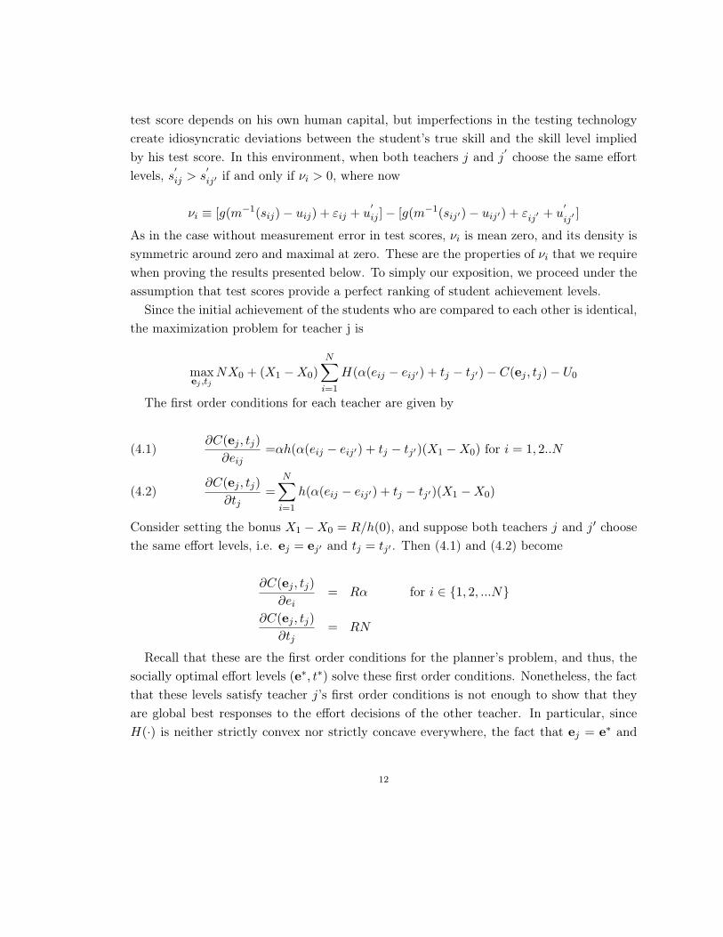
whenever the specific items and format of one assessment can be used to predict the itemsand format present on future assessments.

In order to deter this activity, the education authority could instruct its testing agencyto administer exams each fall and spring that cover the same topics but contain differentquestions in different formats. However, as we noted in the introduction, standard methodsdo not allow education authorities to place assessments on a common scale if they containno common items and are given at different points in time.11

Further, taking as given any set of procedures that a testing agency may employ toequate assessment forms, teachers face a strong incentive to lobby the testing agency toalter the content of the spring assessment or its scaling in a manner that weakens effortincentives. Concerns about scale manipulation may seem far fetched to some, but theliterature on the implementation of state accountability systems under NCLB containssuggestive evidence that several states inflated the growth in their reported proficiency ratesby making assessments easier without making appropriate adjustments to how exams arescored or by introducing new assessments and equating the scales between the old and newassessments in ways that appear generous to the most recent cohorts of students.12 Teachersfacing the relative performance pay scheme described in section 3 above would benefit ifthey could secretly pressure the testing agency to correctly equate various assessments butthen report spring scores that are artificially compressed. If teachers believe their lobbyingefforts have been successful, each individual teacher’s incentive to provide effort will bereduced, but teachers will still collect the same expected salary. Teachers can achieve asimilar result by convincing the testing agency to manipulate the content of the springexam in a way that compresses scores.

Appendix A fleshes out in more detail the ways that scale dependent systems like therelative performance pay system described above invite coaching and scale manipulation.Given these concerns, we explore the optimal design of teacher incentives in a setting wherewe require the education authority to employ incentive schemes that are scale invariant, i.e.schemes that rely only on ordinal information and can thus be implemented without regardto scaling. In order to develop intuition for our results, we first consider ordinal contests

11Equating methods based on the assumption that alternate forms are given to populations with the samedistribution of achievement are not appropriate for repeated samples taken over time from a given populationof students since the hope is that the distribution of true achievement improves over time for a given set ofstudents.12See Peterson and Hess (2006) and Cronin et al (2007). As another example, in 2006, the state of Illinoissaw dramatic and incredible increases in proficiency rates that were coincident with the introduction of anew assessment series. See ISBE (2006).

10

among pairs of teachers. We then examine tournaments that involve simultaneous compe-tition among large numbers of teachers and show that such tournaments are essentially apay for percentile scheme.

Consider a scheme where each teacher j competes against one other teacher and theresults of this contest determine bonus pay for teacher j and her opponent. Teacher j doesnot know who her opponent will be when she makes her effort choices. She knows onlythat her opponent will be chosen from the set of other teachers in the system and that heropponent will be facing the same compensation scheme that she faces. Let each teacherreceive a base pay of X0 per student, and at the end of the year, match teacher j withsome other teacher j′ and pay teacher j a bonus (X1 −X0) for each student i whose scoreis higher than the corresponding student in teacher j′’s class, i.e. if s′ij ≥ s′ij′ . The totalcompensation for teacher j is thus

NX0 + (X1 −X0)N∑i=1

I(s′ij ≥ s′ij′)

where I(A) is an indicator that equals 1 if event A is true and 0 otherwise. Because ordinalcomparisons determine all payoffs, teacher behavior and teacher welfare are invariant toany re-scaling of the assessment results that preserves ordering.

For each i ∈ 1, 2...N , let us define a new variable νi = εij − εij′ as the difference inthe shock terms for students in the two classes whose initial human capital is ai. If bothteachers j and j

′ choose the same effort levels, then s′ij > s

′ij′ if and only if νi > 0. Let

H(x) ≡ Pr(νi ≤ x) denote the distribution of νi. We assume H(·) is twice differentiableand define h(x) = dH(x)/dx. Since εij are i.i.d, νi has mean zero, and h(·) is symmetricaround zero. Moreover, h(x) attains its maximum at x = 0.13

In our framework, νi is the only source of uncertainty in our contests, and since test scoresrank students perfectly according to their true achievement levels, vi only reflects shocksto true achievement. Some readers may wonder how our analyses change if we consider anenvironment in which test scores rank students according to their true achievement levelswith error. Incorporating measurement error makes our notation more cumbersome, butas we now argue, the presence of measurement error in test scores does not alter our basicresults if we assume that the errors in measurement are drawn independently from the samedistribution for all students.

Suppose test scores are given by s = m(a+ u) where u is a random variable with meanzero drawn independently for all students from a common distribution, i.e. each student’s

13See Vogt (1983).11

test score depends on his own human capital, but imperfections in the testing technologycreate idiosyncratic deviations between the student’s true skill and the skill level impliedby his test score. In this environment, when both teachers j and j′ choose the same effortlevels, s′ij > s

′ij′ if and only if νi > 0, where now

νi ≡ [g(m−1(sij)− uij) + εij + u′ij ]− [g(m−1(sij′)− uij′) + εij′ + u

′

ij′]

As in the case without measurement error in test scores, νi is mean zero, and its density issymmetric around zero and maximal at zero. These are the properties of νi that we requirewhen proving the results presented below. To simply our exposition, we proceed under theassumption that test scores provide a perfect ranking of student achievement levels.

Since the initial achievement of the students who are compared to each other is identical,the maximization problem for teacher j is

maxej ,tj

NX0 + (X1 −X0)N∑i=1

H(α(eij − eij′) + tj − tj′)− C(ej , tj)− U0

The first order conditions for each teacher are given by

∂C(ej , tj)∂eij

=αh(α(eij − eij′) + tj − tj′)(X1 −X0) for i = 1, 2..N(4.1)

∂C(ej , tj)∂tj

=N∑i=1

h(α(eij − eij′) + tj − tj′)(X1 −X0)(4.2)

Consider setting the bonus X1 −X0 = R/h(0), and suppose both teachers j and j′ choosethe same effort levels, i.e. ej = ej′ and tj = tj′ . Then (4.1) and (4.2) become

∂C(ej , tj)∂ei

= Rα for i ∈ {1, 2, ...N}

∂C(ej , tj)∂tj

= RN

Recall that these are the first order conditions for the planner’s problem, and thus, thesocially optimal effort levels (e∗, t∗) solve these first order conditions. Nonetheless, the factthat these levels satisfy teacher j’s first order conditions is not enough to show that theyare global best responses to the effort decisions of the other teacher. In particular, sinceH(·) is neither strictly convex nor strictly concave everywhere, the fact that ej = e∗ and

12

tj = t∗ satisfy the first order conditions does not imply that these effort choices are optimalresponses to teacher j′ choosing the same effort levels.

Appendix B provides proofs for the following two propositions that summarize our mainresults for two teacher contests:

Proposition 1: Let εij denote a random variable with a symmetric unimodal density andmean zero, and let εij=σεij. There exists σ such that ∀σ > σ, both teachers choosing thesocially optimal effort levels (e∗, t∗) is a pure strategy Nash equilibrium of the two teachercontest.

The intuition behind the variance restriction in this proposition is straightforward. In anygiven contest, both effort choices and chance play a role in determining the winner. Whenchance plays a small role, (e∗, t∗) will not be a best response to the other teacher choosing(e∗, t∗) unless prizes are small because, when chance plays a small role, the derivative ofthe probability of winning of given contest with respect to teacher effort is large. In fact,the bonus, R

h(0) , tends to zero as σ → 0. The restriction on σ in Proposition 1 is neededto rule out cases where, given the other teacher is choosing (e∗, t∗), the bonus is so smallthat teacher j’s expected gain from responding with (e∗, t∗) as opposed to some lower effortlevel does not cover the incremental effort cost.14 However, if the element of chance in thesecontests is important enough, a pure strategy Nash equilibrium exists which involves bothteachers choosing the socially optimal effort vectors, (e∗, t∗), and Proposition 2 adds thatthis equilibrium is unique.

Proposition 2: In the two teacher contest, whenever a pure strategy Nash equilibriumexists, it involves both teachers choosing the socially optimal effort levels (e∗, t∗).

Taken together, our propositions imply that our tournament scheme can elicit efficienteffort from teachers who compete against each other in seeded competitions. Thus, theefficiency properties that Lazear and Rosen (1981) derived for a setting in which two playersmake one effort choice and compete in a single contest carry over to settings in which twoplayers make multiple effort choices and engage in many contests simultaneously. This istrue even though some of these effort choices affect the outcome of many contests.

Finally, to ensure that teachers are willing to participate in this scheme, we need to makesure that

NX0 +RN

2h(0)− C(e∗, t∗) ≥ U0

14Lazear and Rosen (1981) require a similar condition for existence in their single task, two person game.13

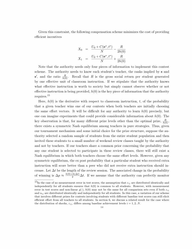
Given this constraint, the following compensation scheme minimizes the cost of providingefficient incentives

X0 =U0 + C(e∗, t∗)

N− R

2h(0)

X1 =U0 + C(e∗, t∗)

N+

R

2h(0)

Note that the authority needs only four pieces of information to implement this contestscheme. The authority needs to know each student’s teacher, the ranks implied by s ands′, and the ratio R

h(0) . Recall that R is the gross social return per student generatedby one effective unit of classroom instruction. If we stipulate that the authority knowswhat effective instruction is worth to society but simply cannot observe whether or noteffective instruction is being provided, h(0) is the key piece of information that the authorityrequires.15

Here, h(0) is the derivative with respect to classroom instruction, t, of the probabilitythat a given teacher wins one of our contests when both teachers are initially choosingthe same effort vectors. It will be difficult for any authority to learn h(0) precisely, butone can imagine experiments that could provide considerable information about h(0). Thekey observation is that, for many different prize levels other than the optimal prize, R

h(0) ,there exists a symmetric Nash equilibrium among teachers in pure strategies. Thus, givenour tournament mechanism and some initial choice for the prize structure, suppose the au-thority selected a random sample of students from the entire student population and theninvited these students to a small number of weekend review classes taught by the authorityand not by teachers. If our teachers share a common prior concerning the probability thatany one student is selected to participate in these review classes, there will still exist aNash equilibrium in which both teachers choose the same effort levels. However, given anysymmetric equilibrium, the ex post probability that a particular student who received extrainstruction will score better than a peer who did not receive extra instruction should in-crease. Let ∆t be the length of the review session. The associated change in the probabilityof winning is ∆p ≈ h(0)+h(∆t)

2 ∆t. If we assume that the authority can perfectly monitor

15In the case of no measurement error in test scores, the assumption that εij are distributed identically andindependently for all students ensures that h(0) is common to all students. However, with measurementerror in test scores and non-linear g(·), h(0) may not be the same for all comparison sets even if both εij

and uij are distributed identically and independently for all students. In this case, a variation of our schemethat involves different prizes for contests involving students with different baseline test scores can still elicitefficient effort from all teachers to all students. In section 6, we discuss a related result for the case wherethe distribution of shocks, εij , differs among baseline achievement levels i = 1, 2..N .

14

instruction quality during these experimental sessions and if we choose a ∆t that is a trivialintervention relative to the range of shocks, ε, that affect achievement during the year, thesample mean of ∆p

∆t provides a useful approximation for h(0).16

The two-teacher contest system described here elicits efficient effort from teachers and,because it relies only on ordinal information, can be implemented without equating scoresscores from different assessment forms. Further, since equating is not required, our schemeallows the education authority to employ completely new assessment forms at each point intime and thereby remove opportunities for teachers to coach students for specific questionsor question formats based on previous assessments. Our scheme is also robust againstefforts to weaken performance incentives by corrupting assessment scales, since the mappingbetween outcomes and reward pay is scale invariant.

5. Pay for Percentile

While our two-teacher contests address some ways that teachers can manipulate incentivepay systems, the fact that each teacher plays against a single opponent may raise concernsabout a different type of manipulation. Recall, we assume that the opponent for teacherj is announced at the end of the year after students are tested. Thus, some teachersmay respond to this system by lobbying school officials to be paired with a teacher whosestudents performed poorly. If one tried to avoid these lobbying efforts by announcing thepairs of contestants at the beginning of the year, then one would worry about collusionon low effort levels within pairs of contestants. We now turn to performance contests thatinvolve large numbers of teachers competing anonymously against one another. We expectthat collusion on low effort among teachers is less of a concern is this environment.

Suppose that each teacher now competes against K teachers who also have N students.Each teacher knows that K other teachers will be drawn randomly from the populationof teachers with similar classrooms to serve as her contestants, but teachers make theireffort choices without knowing whom they are competing against. We assume that teachersreceive a base salary of X0 per student and a constant bonus of (X1−X0) for each contestshe wins.17 In this setting, teacher j’s problem is

16Our production technology implicitly normalizes the units of ε so that shocks to achievement can bethought of in terms of additions to or deletions from the hours of effective classroom instruction t studentsreceive. Further, because R is the social value of a unit of effective instruction time, the prize R

h(0)determined

by this procedure is the same regardless of the units used to measure instruction time, e.g. seconds, minutes,hours.17A constant prize per contest is not essential for eliciting efficient effort, but we view it as natural giventhe symmetry of the contests.

15

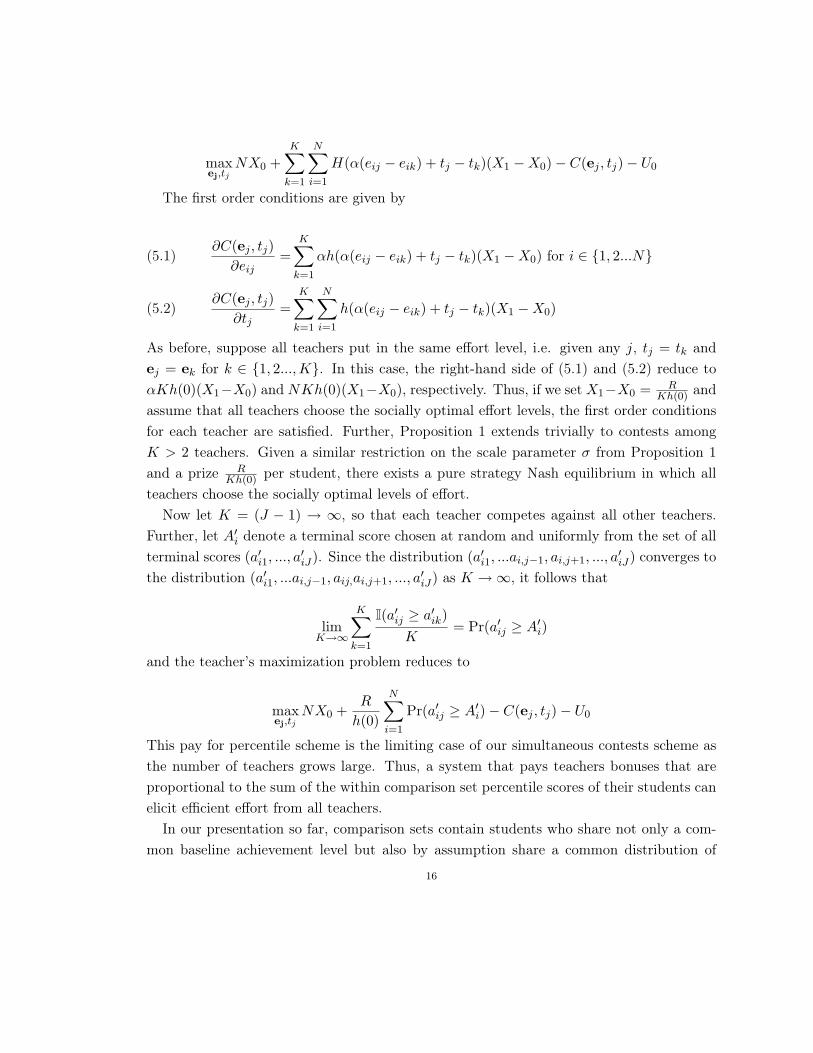
maxej,tj

NX0 +K∑k=1

N∑i=1

H(α(eij − eik) + tj − tk)(X1 −X0)− C(ej , tj)− U0

The first order conditions are given by

∂C(ej , tj)∂eij

=K∑k=1

αh(α(eij − eik) + tj − tk)(X1 −X0) for i ∈ {1, 2...N}(5.1)

∂C(ej , tj)∂tj

=K∑k=1

N∑i=1

h(α(eij − eik) + tj − tk)(X1 −X0)(5.2)

As before, suppose all teachers put in the same effort level, i.e. given any j, tj = tk andej = ek for k ∈ {1, 2...,K}. In this case, the right-hand side of (5.1) and (5.2) reduce toαKh(0)(X1−X0) and NKh(0)(X1−X0), respectively. Thus, if we set X1−X0 = R

Kh(0) andassume that all teachers choose the socially optimal effort levels, the first order conditionsfor each teacher are satisfied. Further, Proposition 1 extends trivially to contests amongK > 2 teachers. Given a similar restriction on the scale parameter σ from Proposition 1and a prize R

Kh(0) per student, there exists a pure strategy Nash equilibrium in which allteachers choose the socially optimal levels of effort.

Now let K = (J − 1) → ∞, so that each teacher competes against all other teachers.Further, let A′i denote a terminal score chosen at random and uniformly from the set of allterminal scores (a′i1, ..., a

′iJ). Since the distribution (a′i1, ...ai,j−1, ai,j+1, ..., a

′iJ) converges to

the distribution (a′i1, ...ai,j−1, aij,ai,j+1, ..., a′iJ) as K →∞, it follows that

limK→∞

K∑k=1

I(a′ij ≥ a′ik)K

= Pr(a′ij ≥ A′i)

and the teacher’s maximization problem reduces to

maxej,tj

NX0 +R

h(0)

N∑i=1

Pr(a′ij ≥ A′i)− C(ej , tj)− U0

This pay for percentile scheme is the limiting case of our simultaneous contests scheme asthe number of teachers grows large. Thus, a system that pays teachers bonuses that areproportional to the sum of the within comparison set percentile scores of their students canelicit efficient effort from all teachers.

In our presentation so far, comparison sets contain students who share not only a com-mon baseline achievement level but also by assumption share a common distribution of

16

baseline achievement among their peers. However, given the separability we impose on thehuman capital production function in equation (2.1) and the symmetry we impose on thecost function, student i’s comparison set need not be restricted to students with similarclassmates. For any given student, we can form a comparison set by choosing all studentsfrom other classrooms who have the same baseline achievement level regardless of the dis-tributions of baseline achievement among their classmates. This result holds because thesocially optimal allocation of effort (e∗, t∗) dictates the same level of classroom instructionand tutoring effort from all teachers to all students regardless of the baseline achievementof a given student or the distribution of baseline achievement in his class.

Thus, given the production technology that we have assumed so far, pay for percentile canbe implemented quite easily and transparently in any large school system. The educationauthority can form one comparison set for each distinct level of baseline achievement andthen assign within comparison set percentiles based on the end of year assessment results. Inthe following section, we consider more general production functions. In these environments,comparison sets must condition on classroom characteristics. We show that the existenceof peer effects, instructional spillovers and other forces that we have not modeled to thispoint do not alter the efficiency properties of pay for percentile but simply complicate thetask of constructing comparison sets.

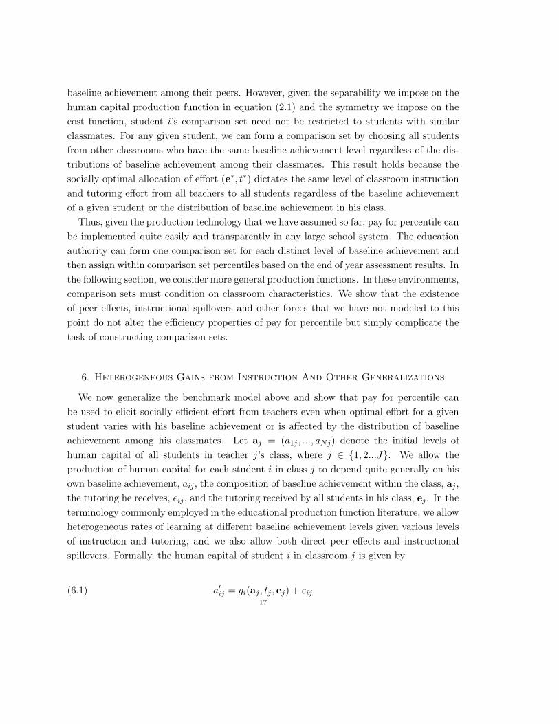
6. Heterogeneous Gains from Instruction And Other Generalizations

We now generalize the benchmark model above and show that pay for percentile canbe used to elicit socially efficient effort from teachers even when optimal effort for a givenstudent varies with his baseline achievement or is affected by the distribution of baselineachievement among his classmates. Let aj = (a1j , ..., aNj) denote the initial levels ofhuman capital of all students in teacher j’s class, where j ∈ {1, 2...J}. We allow theproduction of human capital for each student i in class j to depend quite generally on hisown baseline achievement, aij , the composition of baseline achievement within the class, aj ,the tutoring he receives, eij , and the tutoring received by all students in his class, ej . In theterminology commonly employed in the educational production function literature, we allowheterogeneous rates of learning at different baseline achievement levels given various levelsof instruction and tutoring, and we also allow both direct peer effects and instructionalspillovers. Formally, the human capital of student i in classroom j is given by

(6.1) a′ij = gi(aj , tj , ej) + εij17

Because gi (·, ·, ·) is indexed by i, this formulation allows different students in the sameclass to benefit differently from the same environmental inputs, i.e. from other classmates,classroom instruction, and individual tutoring of other students in the class. Nonetheless,we place three restrictions on gi (·, ·, ·): the first derivatives of gi (·, ·, ·) with respect toeach dimension of effort are finite everywhere, gi (·, ·, ·) is weakly concave, and gi (·, ·, ·)depends on class identity, j, only through teacher efforts. Our concavity assumption placesrestrictions on forms that peer effects and instructional spillovers may take. Our assumptionthat j enters only through teacher effort choices implies that, for any two classrooms (j, j′)with the same composition of baseline achievement, if the two teachers in question choosethe same effort levels, i.e. tj = tj′ and ej = ej′ , the expected human capital for any twostudents in different classrooms who share the same initial achievement, i.e. aij = aij′ ,will be the same. Given this property and the fact that the cost of effort is the same forboth teachers, we can form comparison sets at the classroom level and guarantee that allcontests are properly seeded.

For now, we will continue to assume the εij are pairwise identically distributed acrossall pairs (i, j), although we comment below on how our scheme can be modified if thedistribution of εij can vary across students with different baseline achievement levels. Insection 2, given our separable form for gi (·, ·, ·), we could interpret the units of εij in terms ofadditions to or deletions from effective classroom instruction time. Given the more generalformulation of gi (·, ·, ·) here, this interpretation need no longer apply in all classrooms.Thus, the units of εij can now only be interpreted as additions to or deletions from thestock of student skill.

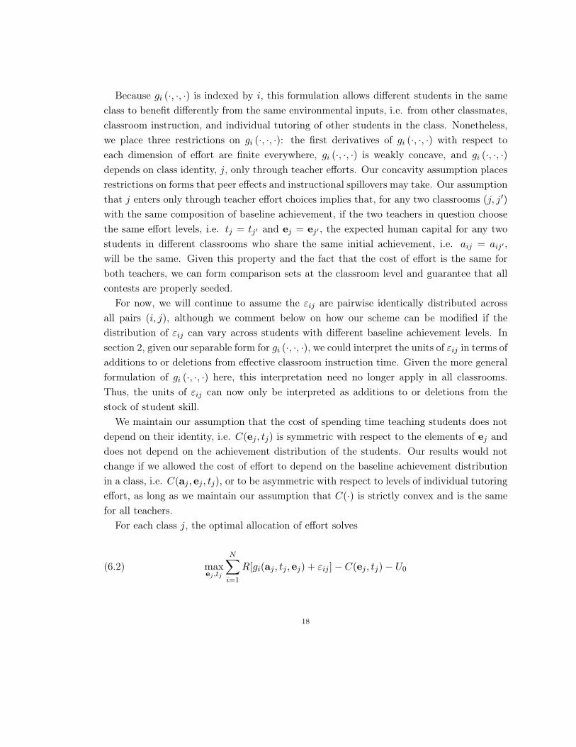
We maintain our assumption that the cost of spending time teaching students does notdepend on their identity, i.e. C(ej , tj) is symmetric with respect to the elements of ej anddoes not depend on the achievement distribution of the students. Our results would notchange if we allowed the cost of effort to depend on the baseline achievement distributionin a class, i.e. C(aj , ej , tj), or to be asymmetric with respect to levels of individual tutoringeffort, as long as we maintain our assumption that C(·) is strictly convex and is the samefor all teachers.

For each class j, the optimal allocation of effort solves

(6.2) maxej ,tj

N∑i=1

R[gi(aj , tj , ej) + εij ]− C(ej , tj)− U0

18

Since gi(·, ·, ·) is concave for all i and C(·) is strictly convex, this problem is strictlyconcave, and the first-order conditions are both necessary and sufficient for an optimum.These are given for all j by

∂C(ej , tj)∂eij

= RN∑m=1

∂gm(aj , tj , ej)∂eij

for i ∈ {1, 2...N}

∂C(ej , tj)∂tj

= RN∑m=1

∂gm(aj , tj , ej)∂tj

For any composition of baseline achievement, there will be a unique(e∗j , t

∗j

)that solves

these equations. However, this vector will differ for classes with different compositions, aj,and the tutoring effort, eij , for each student will generally differ across students in the sameclass if the students have different initial achievement levels.

We now argue that the same pay for percentile scheme we described above will continueto elicit socially optimal effort vectors from all teachers. The bonus scheme is the same asbefore, and again, each student will be compared to all students with the same baselineachievement who belong to one of the K other classrooms in his comparison set.18

Assume that we offer each teacher j a base pay of X0 per student, and a bonus X1 −X0 = R

Kh(0) for each student in any comparison class k ∈ {1, 2...K} who scores belowhis counterpart in teacher j’s class on the spring assessment. Teacher j’s problem can beexpressed as follows:

maxej,tj

NX0 + (X1 −X0)K∑k=1

N∑i=1

H(gi(aj , tj , ej)− gi(ak, tk, ek))− C(ej , tj)

The first order conditions for teacher j are

∂C(ej , tj)∂eij

= (X1 −X0)K∑k=1

N∑m=1

∂gm(aj , tj , ej)∂eij

h(gm(aj , tj , ej)− gm(ak, tk, ek)) ∀i ∈ {1, 2...N}

∂C(ej , tj)∂tj

= (X1 −X0)K∑k=1

N∑m=1

∂gm(aj , tj , ej)∂tj

h(gm(aj , tj , ej)− gm(ak, tk, ek))

18As we note at the end of the previous section, this composition restriction on comparison sets is nowbinding. We noted in the previous section that when gi (·, ·, ·) is separable in ai and teacher’s effort, thecomparison set for student i may contain any student with the same baseline achievement regardless of thecomposition of baseline achievement in this student’s class.

19

If all teachers provide the same effort levels, these first order conditions collapse to theplanner’s first order conditions. If we assume that other teachers are choosing the sociallyoptimal levels of effort, then for large enough σ, these first-order conditions are necessaryand sufficient for an optimal response. The proof of Proposition 1 in Appendix B establishesthat there exists a Nash equilibrium such that all teachers choose the first best effort levelsin response to a common prize structure in this more general setting as well. However, eventhough the bonus rate is the same for all teachers, base pay will not be. Because sociallyefficient effort levels vary with classroom composition, the level of base pay required tosatisfy the teachers’ participation constraints will be a function of the specific distributionof baseline achievement that defines a comparison set or a set of competing classrooms.

Here, pay for percentile amounts to competition among teachers within leagues definedby classroom type. These leagues offer properly seeded contests even in the presence ofpeer effects and heterogeneity in student learning rates. Further, because the competitioninvolves all students in each classroom, teachers internalize the consequences of instructionalspillovers.

In practice, it may be impossible to form large comparison sets containing classroomswith identical distributions of baseline achievement. Nevertheless, it may still be possible toimplement our system using a large set of quantile regression models that allow researchersto create, for any set of baseline student and classroom characteristics, a set of predictedscores associated with each percentile in the conditional distribution of scores. Given apredicted score distribution for each individual student that conditions on his own baselineachievement and the distribution of baseline achievement among his classmates, educationauthorities can assign a conditional percentile score to each student and then form percentileperformance indices at the classroom level.19

As we noted above, even with our more general formulation for gi (·, ·, ·), the optimal prizestructure does not vary with baseline achievement and does not depend on the functionalform of gi (·, ·, ·). This result hinges on our assumption that the distribution of εij , andthus h(0), does not vary among students. When the production function, gi (·, ·, ·), varieswith achievement level i, experimental estimates of the effect of additional instruction onthe probability of winning seeded contests cannot be used to test the hypothesis that h(0)is constant across different baseline achievement levels.20 Further, even if h(0) is the same

19See Briggs and Betebenner (2009) for an example of how these conditional percentile scores can becalculated in practice.20In the experiment we described at the end of section 4, students are given a small amount of extra

instruction, and the experiment identifies h(0)∂a

′ij

∂tj, which equals h(0) given the linear technology assumed

in Section 2. If we ran separate experiments of this type for each baseline achievement level, we could not20

for all pairwise student contests regardless of baseline achievement levels, the process ofdiscovering h(0) given the more general technology g (·, ·, ·) is a little more involved thanthe process described in section 4. Given this more general technology, R is no longer thevalue of instruction time provided to any student. R must now be interpreted as the valueof the skills created when one unit of instruction time is devoted to a particular type ofstudent in a specific type of classroom. Thus, attempts to learn h(0) based on experimentslike those described in section 4 must be restricted to a specific set of students who allhave the same baseline achievement level, the same peers, and some known baseline levelof instruction and tutoring.

If one assumes that h(0) differs with baseline achievement, the authority can still elicitefficient effort by using a pay for percentile scheme that offers different prizes for winningdifferent contests i.e. rates of pay for percentile, R

Khi(0) , that are specific to each level ofbaseline achievement. The key implication of our analyses is that performance pay foreducators should be based on ordinal rankings of student outcomes within properly chosencomparison sets. Details concerning the determination of the prize levels associated withdifferent contests hinge on details concerning the nature of education production and shocksto human capital accumulation.

7. Lessons for Policy Makers

In the previous sections, we describe a simultaneous contest mechanism that can elicitefficient effort from teachers and is robust to certain types of manipulation. In this section,we shift our attention to existing performance pay systems and analyze them in light ofthe lessons learned from our model. Table 1 summarizes a number of existing pay forperformance schemes that are currently in operation.

Our model yields several insights that are important but have not been fully recognizedin current policy debates. To begin, our analyses highlight the value of peer comparisonsas a means of revealing what efficient achievement targets should be. With the exceptionof TAP and the possible exception of PRP21, all the systems described in Table 1 involvesetting achievement targets for individual students and rewarding teachers for meeting these

use variation in the product hi(0)∂a

′ij

∂tjto test the hypothesis hi(0) = h(0) for all i without knowing how

∂a′ij

∂tjvaries with i.

21PRP instructed teachers to document that their students were making progress “as good or better” thantheir peers. However, PRP involved no system for producing objective relative performance measures, andex post, the high rate of bonus awards raised questions about the leniency of education officials in settingstandards for “as good or better” performance. See Atkinson et al (2009) and Wragg et al (2001).

21

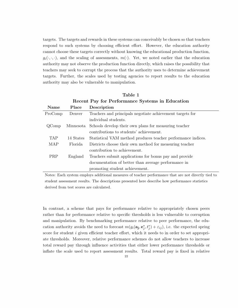
targets. The targets and rewards in these systems can conceivably be chosen so that teachersrespond to such systems by choosing efficient effort. However, the education authoritycannot choose these targets correctly without knowing the educational production function,gi(·, ·, ·), and the scaling of assessments, m(·). Yet, we noted earlier that the educationauthority may not observe the production function directly, which raises the possibility thatteachers may seek to corrupt the process that the authority uses to determine achievementtargets. Further, the scales used by testing agencies to report results to the educationauthority may also be vulnerable to manipulation.

Table 1Recent Pay for Performance Systems in Education

Name Place DescriptionProComp Denver Teachers and principals negotiate achievement targets for

individual students.QComp Minnesota Schools develop their own plans for measuring teacher

contributions to students’ achievement.TAP 14 States Statistical VAM method produces teacher performance indices.MAP Florida Districts choose their own method for measuring teacher

contribution to achievement.PRP England Teachers submit applications for bonus pay and provide

documentation of better than average performance inpromoting student achievement.

Notes: Each system employs additional measures of teacher performance that are not directly tied to

student assessment results. The descriptions presented here describe how performance statistics

derived from test scores are calculated.

In contrast, a scheme that pays for performance relative to appropriately chosen peersrather than for performance relative to specific thresholds is less vulnerable to corruptionand manipulation. By benchmarking performance relative to peer performance, the edu-cation authority avoids the need to forecast m(gi(aj, e∗j , t

∗j ) + εij), i.e. the expected spring

score for student i given efficient teacher effort, which it needs to in order to set appropri-ate thresholds. Moreover, relative performance schemes do not allow teachers to increasetotal reward pay through influence activities that either lower performance thresholds orinflate the scale used to report assessment results. Total reward pay is fixed in relative

22

performance systems, and peforrmance thresholds are endogenously determined throughpeer comparisons.

Among the entries in Table 1, the Value-Added Model (VAM) approach contained in theTAP scheme is the only scheme based on an objective mapping between student test scoresand relative performance measures for teachers. Our percentile performance indices providesummary measures of how often the students in a given classroom perform better thancomparable students in other schools, while VAM models measure the distance between theaverage achievement of students in a given classroom and the average achievement one wouldexpect from these students if they were randomly assigned to different classrooms. Bothschemes produce relative performance indices for teachers, but the VAM approach is moreambitious. VAM indices not only provide a ranking of classrooms according to performance,they also provide measures of the sizes of performance gaps between classrooms.22

Cardinal measures of relative performance are a required component of the TAP approachand related approaches to performance pay for teachers because these systems attempt toboth measure the contributions of educators to achievement growth and reward teachersaccording to these contributions. Donald Campbell (1976) famously claimed that govern-ment performance statistics are always corrupted when high stakes are attached to them,and the contrast between our percentile performance indices and VAM indices suggests thatCampbell’s observation may reflect the perils of trying to accomplish two objectives withone set of performance measures. Systems, like TAP, that try to both provide incentivesfor teachers and produce cardinal measures of educational productivity are likely to doneither well because assessment procedures that enhance an education authority’s capacityto measure achievement growth consistently over time introduce opportunities for teachersto game assessment-based incentive systems. Systems that track achievement must placeresults from a series of assessments on a common scale, and the equating process thatcreates this common scale will not be credible if each assessment contains a completelynew set of questions. The existence of items that have been used on previous assessmentsand will with some probability be repeated on the current assessment invites teachers tocoach students based on the specific items and formats found in the previous assessments,and the existing empirical literature suggests that this type of coaching artificially inflates

22Some VAM practitioners employ functional form assumptions that allow them to produce universal rank-ings of teacher performance and make judgements about the relative performance of two teachers even ifthe baseline achievement distributions in their classes do not overlap. In contrast, our pay for percentilescheme takes seriously the notion that teaching academically disadvantaged students may be a different jobthan than teaching honors classes and provides a context-specific measure of how well teachers are doingthe job they actually have.

23

measures of student achievement growth over time. Further, because it is reasonable toexpect heterogeneity in the extent of these coaching activities across classrooms, there isno guarantee that scale dependent measures of relative performance will actually providethe correct ex post performance ranking over classrooms, and as we noted in Section 4, sys-tems that links rewards to cardinal measures of relative achievement growth may introducepolitical pressures to corrupt equating procedures in ways that compress the distributionof scores, weaken incentives, and contaminate measures of achievement growth.

In contrast, our pay for percentile system elicits effort without creating incentives forcoaching or scale manipulation because it permits the use of new assessments at each pointin time and contains a mapping between assessment results and teacher pay that is scaleinvariant. Given our scheme, if education authorities desire measures of secular changes inachievement or achievement growth over time, they can deploy a second assessment systemthat is scale dependent but with no stakes attached and with only random samples ofschools taking these scaled tests. Educators would face no direct incentives to manipulatethe results of this second assessment system, and thus by separating the tasks of incentiveprovision and output measurement, education authorities would likely do both tasks better.

8. Conclusion

Designing a set of assessments and statistical procedures that will not only allow policymakers to measure secular achievement growth over time but also isolate the contributionof educators and schools to this growth is a daunting task in the best of circumstances.Further, when the results of this endeavor determine rewards and punishments for teachersand principals, some educators respond by taking actions that artificially inflate measuresof student learning. These actions may include coaching students for assessments as wellas lobbying testing agencies concerning how results from different assessments are equated.The high stakes testing literature provides much evidence that teachers coach students forhigh stakes assessments in ways that inflate assessment results relative to student subjectmastery, and the literature on NCLB involves significant debate concerning the integrityof proficiency standards. For example, in 2006 in Illinois, the percentage of eighth gradersdeemed proficient in math under NCLB jumped from 54.3 to 78.2 in one year. This im-provement dwarfs gains typically observed in other years and in other states. Because thisenormous gain was coincident with the introduction of a new series of assessments that

24

were scored on a new scale and then equated to previous tests, the entire episode raisessuspicions about the comparability of proficiency standards across assessment forms.23

Our key insight is that properly seeded contests where winners are determined by therank of student outcomes can provide incentives for efficient teacher effort. Thus, theordinal content of assessment results provides enough information to elicit socially efficienteffort from teachers. This result is important because scale-dependent performance paysystems typically create incentives for educators to coach students based on the questionscontained in previous assessments and to pressure testing agencies to alter the scales used toreport assessment results. These activities are socially wasteful, and they also contaminatemeasurements of student achievement. If policy makers desire cardinal measures of howachievement levels are evolving over time or how the contribution of schools to achievementis evolving over time, they will do a better job of providing credible answers to thesequestions if they address them using a separate measurement system that has no impacton the distribution of rewards and sanctions among teachers and principals.

We are advocating competition based on ranks as the basis for incentive pay systemsthat are immune to specific corruption activities that plague existing performance pay andaccountability systems, but several details concerning how to organize such competitionremain for future research. First and foremost, teachers who teach in the same school shouldnot compete against each other. This type of direct competition could undermine usefulcooperation among teachers. Further, although we have discussed all our results in terms ofcompetition among individual teachers, education authorities may wish to implement ourscheme at the school or school-grade level as a means of providing incentives for effectivecooperation.24

In addition, because our scheme is designed to elicit effort from teachers who share thesame cost of providing effective effort, it may be desirable to have teachers compete onlyagainst other teachers with similar levels of experience, similar levels of support in termsof teacher’s aides, and similar access to computers and other resources.25 While more work

23See ISBE 2006. The new system came online when the state began testing in grades other than grades 3,5, and 8. The introduction of the new assessment system resulted in significant jumps in both reading andmath proficiency in all three grades, but the eighth grade math results are the most suspicious. Cronin etal (2007) contends that other states have inflated proficiency results by compromising the comparability ofassessment scales over time.24This approach is particularly attractive if one believes that peer monitoring within teams is effective. NewYork City’s accountability system currently includes a component that ranks school performance withinleagues defined by student characteristics.25The task of developing a scheme that addresses unobservable differences in teacher talent remains forfuture research. We have not yet characterized the optimal system for both screening teachers and providingeffort incentives based only on the ordinal information in assessments.

25

remains concerning the ideal means of organizing the contests we describe above, our resultsdemonstrate that education authorities can enjoy important efficiency gains from buildingincentive pay systems for teachers that are based on the ordinal outcomes of properly seededcontests and that are completely distinct from any assessment systems used to measure theprogress of students or secular trends in student achievement. In this paper, our educationauthority addresses a moral hazard problem given a homogeneous set of teachers. Furtherresearch is needed to analyze the potential uses of percentile performance indices is settingswhere both the education authority and teachers are learning over time about the relativeeffectiveness of individual teachers.

26

References

[1] Balou, Dale. “Test Scaling and Value-Added Measurement,” NCPI Working paper 2008-23, December,2008.

[2] Briggs, Derek and Damian Betebenner, “Is Growth in Student Achievement Scale Dependent,” mimeo.April, 2009.

[3] Campbell, Donald T. “Assessing the Impact of Planned Social Change," Occasional Working Paper 8(Hanover, N.H.: Dartmouth College, Public Affairs Center, December, 1976).

[4] Cawley, John, Heckman, James, and Edward Vytlacil, "On Policies to Reward the Value Added ofEducators," The Review of Economics and Statistics 81:4 (Nov 1999): 720-727.

[5] Cronin, John, Dahlin, Michael, Adkins, Deborah, and G. Gage Kingsbury. “The Proficiency Illusion."Thomas B. Fordham Institute, October 2007.

[6] Cunha, Flavio and James Heckman. "Formulating, Identifying and Estimating the Technology of Cog-nitive and Noncognitive Skill Formation." Journal of Human Resources 43 (Fall 2008): 739-780.

[7] Gootman, Elissa. “In Brooklyn, Low Grade for a School of Successes." New York Times, September12, 2008.

[8] Holmstrom, Bengt and Paul Milgrom. “Multitask Principal-Agent Analyses: Incentive Contracts, AssetOwnership and Job Design," Journal of Law, Economics and Organization, 7 (January 1991) 24-52.

[9] Illinois State Board of Education. 2006 Illinois State Report Card, 2006.[10] Jacob, Brian. “Accountability Incentives and Behavior: The Impact of High Stakes Testing in the

Chicago Public Schools,” Journal of Public Economics 89:5 (2005), 761-796.[11] Jacob, Brian and Steven Levitt. “Rotten Apples: An Investigation of the Prevalence and Predictors of

Teacher Cheating,” Quarterly Journal of Economics 118:3 (2003) 843-877.[12] Klein, Stephen, Hamilton, Laura, McCaffrey, Daniel, and Brian Stecher. “What Do Test Scores in

Texas Tell Us?” Rand Issue Paper 202 (2000).[13] Koretz, Daniel M. “Limitations in the Use of Achievement Tests as Measures of Educators’ Productiv-

ity,” Journal of Human Resources 37:4 (2002) 752-777.[14] Lazear, Edward. “Educational Production.” Quarterly Journal of Economics 16:3 (Aug 2001) 777-803.[15] Lazear, Edward and Sherwin Rosen. “Rank Order Tournaments as Optimum Labor Contracts,” Journal

of Political Economy 89:5 (Oct 1981): 841-864.[16] Peterson, Paul and Frederick Hess. “Keeping an Eye on State Standards: A Race to the Bottom,”

Education Next (Summer 2006) 28-29.[17] Vogt, H. “Unimodality in Differences,” Metrika 30:1 (Dec 1983) 165-170.

27

9. APPENDICES

Appendix A

We argue that our pay for percentile scheme is advantageous because it is robust againstcertain forms of coaching and scale manipulation. Because we do not model coaching andscale manipulation explicitly in our main analyses, this Appendix provides a more preciseexplanation of what we mean by coaching and scale manipulation. To simplify notation,we assume g (a) = 0 for all a, so that

(9.1) a′ij = tj + αeij + εij

We can think of this as a special case of our environment in which all students enjoy thesame baseline achievement level.

Coaching. First, we model coaching using a simple version of Holmstrom and Milgrom’s(1991) multi-tasking model. Here, we define coaching as the time that teachers devote tomemorization of the answers to questions on previous exams, instruction on test takingtechniques that are specific to the format of previous exams, or test taking practice sessionsthat involve repeated exposure to previous exam questions. These activities may createhuman capital, but we assume that these activites are socially wasteful because they createless human capital per hour than classroom time devoted to effective comprehensive in-struction. However, teachers still have an incentive to coach if coaching has a large enougheffect on test scores.

Suppose that in addition to the effort choices ej and tj , teachers can also engage incoaching. Denote the amount of time teacher j spends on this activity by τj . To facilitateexposition, assume τj and tj are perfectly substitutable in the teacher’s cost of effort, sinceboth represent time working with the class as a whole. That is, the cost of effort for teacherj is given by C (ej , tj + τj), where C (·, ·) is once again assumed to be convex.

We allow τj to affect human capital, but with a coefficient θ that is less than 1, i.e., wereplace (9.1) with

a′ij = tj + θτj + αeij + εij

Hence, τj is less effective in producing human capital than general classroom instructiontj . At the same time, suppose τj helps to raise the test score for a student of a givenachievement level by improving their chances of getting specific items correct on a test.That is,

s′ij = m(a′ij + µτj)28

where µ ≥ 0 reflects the productivity of coaching in improving test scores for a studentwith a given level of human capital.

For any compensation scheme that is increasing in s′ij , teachers will choose to coachrather than teach if θ + µ > 1. It seems reasonable to assert that µ is an increasingfunction of the fraction of items on a given assessment that are repeated items from previousassessments. The return to coaching kids on the answers to specific questions or how todeal with questions in specific formats should be increasing in the frequency with whichthese specific questions and formats appear on the future assessments. Because coaching issocially wasteful, the education authority would like to make each year’s test so differentfrom previous exams that θ+µ < 1 and more generally so that µ is close to zero. However,any attempt to minimize the use of previous items will make it more difficult to placescores on a common scale across assessments, and in the limit, standard psychometrictechniques cannot be used to equate two assessments given at different points in time,and thus presumably to populations with different distributions of human capital, if theseassessments contain no common items. Thus, in practice, scale-dependent compensationschemes create opportunities for coaching because they require the repitition of items overtime. Scale-invariant compensation schemes, such as our pay for percentile system, canbe used to reduce coaching because these schemes can employ a series of assessments thatcontain no repeated items.

Although we chose to interpret τj as coaching, teachers may try to raise test scores byengaging in other socially inefficient activities. The ordinal system we propose can helpeducation authorities remove incentives for teachers to coach students concerning specificquestions that are likely to appear on the next assessment. However, in any assessmentbased performance pay system, individual teachers can often increase their reward payby taking actions that are hidden from the education authority. The existing empiricalliterature suggests that these actions take many forms, e.g. manipulating the population ofstudents tested and changing students’ answers before their tests are graded. Our schemeis less vulnerable to coaching, but no less vulnerable to these types of distortions.

Scale Manipulation. Assume that the education authority contracts with a testing agencyto test students and report the results of the tests. The testing agency knows the true map-ping between test results and human capital, and thus the authority can contract with thetesting agency to report scores in units of human capital, so that

s = m(a) = a29

The educational authority then announces the rule by which teachers will be compen-sated. This rule is a mapping from the set of all reported test scores to the set of incomes foreach teacher. Let xj (s′1, ..., s

′J) equal teacher j′s income under the announced rule, where

s′j = (s1j , ..., sNj) is the vector of scores of all students in class j at the end of the year.We argue in Section 3 that, if the educational authority knows that the scores are scaled inunits of human capital, it can maximize total surplus from the production of human capitalby adopting the following relative performance pay scheme

(9.2) xj(s′1, ..., s

′J

)= NX0 +R

N∑i=1

s′ij − 1J

J∑j=1

s′ij

where s′ = m (a′) = a′ .

We assume that, after x (·) is announced, the teachers have opportunity to collectivelylobby the testing agency to report scores on a different scale, which we restrict to take theform

s = m (a) = λa+ φ

where λ > 0, which implies that any manipulation must preserve ordering. Our concern isscaling, not errors in measurement. The teachers or their union may engage in this type ofmanipulation by lobbying the testing agency to choose sets of questions that are less dis-criminating and do not capture the true extent of human capital differences among students,or they may lobby the testing agency to falsely equate scores from current assessments tosome established baseline scale.

Note that (9.2) is robust against efforts to inflate scores by choosing φ > 0 becausepayments are based on relative performance. However, the teachers can still benefit fromconvincing the testing agency to choose λ < 1. Given this scheme or other symmetric,relative compensation schemes, all teachers face the same incentives and will thus putin the same effort. This implies that, if the testing agency reports m(a) instead m(a),the expected teacher payoff from (9.2) equals NX0 − C(ej , tj), where (ej , tj) denotes thecommon level of effort teachers choose in response to the scale that they have convinced thetesting agency to employ. Any manipulation of the scale that induces teachers to coordinateon a lower common level of effort will make them all better off. To see that teachers cancoordinate on less effort by manipulating λ, note that under (9.2), each risk neutral teacher

30

faces the problem,

maxej ,tj

NX0 +N∑i=1

R[λ(tj + αeij)− constant

]− C (ej , tj)

and thus (ej , tj) are decreasing functions of λ.Of course, just because teachers have an incentive to manipulate λ, does not mean that

they can do so without being detected by the authority. Recall that, in equilibrium, allteachers put in the same effort, and thus, any variation in scores is due to εij . Thus, if theeducation authority knows the distribution of εij , it can detect whether λ = 1 by comparingthe standard deviation of test scores with the standard deviation of εij .

However, if the education authority is uncertain about the distribution of εij but teachersknow the distribution, the education authority may be unable to detect λ < 1. Supposethere are two states of the world, each equally likely, which differ in the dispersion of theshock term, εij . In the first state, the shock is εij , as above, and in the second state the shockis scaled up by a constant σ > 1. If teachers observe that they are in the second state of theworld, they can set λ = 1/σ (and choose φ appropriately) so that the distribution of testscores is identical to the distribution of test scores in the first state of the world when λ = 1.Thus, under the relative pay for perfromance scheme above, teachers could manipulate thescale without being detected, and they would benefit from this manipulation.

By contrast, our pay-for-percentile scheme has the advantage of not being vulnerable tothis type of manipulation. By construction, changing the scale has no effect on the compen-sation teachers would earn under pay for percentile. Our scheme does require identifyingwhich of the two states of the world we are in, since h (0) will differ in these states. However,the procedure we suggest for recovering h (0) works in either state.26

Appendix B: Proofs

Proposition 1: Let εij denote a random variable with a symmetric unimodal density andmean zero, and let εij=σεij. There exists σ such that ∀σ > σ, both teachers choosing thesocially optimal effort levels (e∗, t∗) is a pure strategy Nash equilibrium of the two teachercontest.

26Note that there may be scale-dependent schemes that still elicit first best. For example, if the educationauthority offers a higher base pay whenever the dispersion of scores is high, it can provide incentives thatdissuade teachers from distorting the scale. Since a change in base pay does not affect the incentive to putin effort, such a scheme can elicit first best effort.

31

Proof of Proposition 1: Our proof will be for the general production function a′ij =gi(a, tj , ej), which includes the separable case in Section 2 as a special case.

Define νij = εij − εij′ , and let H(x) ≡ Pr(vi ≤ x). Then, H(x) = H(x/σ). Similarly, we

have h(x) ≡ dH(x)dx

=1σh(x/σ). Note that

h(0) =1σh(0).

Consider the probability that teacher j wins the contest over student i when her opponentchooses the socialy optimal vector of effort, (e∗, t∗). Let a = aj = aj′ . Then this probabilityis given by

H(gi(a, tj , ej)− gi(a, t∗, e∗)) =∫ gi(a,tj ,ej)−gi(a,t

∗,e∗)

−∞h(x)dx

=∫ gi(a,tj ,ej)−gi(a,t

∗,e∗)

−∞

1σh(x/σ)dx

Because NX0 and U0 are constants, the solution to teacher j’s problem also solves themaximization problem

maxej ,tj

(X1 −X0)N∑i=1

H(gi(a, tj , ej)− gi(a, t∗, e∗))− C(ej , tj)

If we set X1 −X0 = R/h(0), and use the fact that h(x)h(0) =

eh(x/σ)eh(0)this problem reduces to

(9.3) maxej ,tj

RN∑i=1

[∫ gi(a,tj ,ej)−gi(a,t∗,e∗)

−∞

h(x/σ)

h(0)dx

]− C(ej , tj)

We first argue that the solution to this problem is bounded in a way that does not dependon σ. Observe that the objective function (9.3) is nonnegative at (e, t)=(0,0). Next, since

h (·) has a peak at zero, it follows thath(x/σ)

h(0)≤ 1 for all x and so

∫ gi(a,tj ,ej)−gi(a,t∗,e∗)

−∞

h(x/σ)

h(0)dx =

∫ gi(a,0,0)−gi(a,t∗,e∗)

−∞

h(x/σ)

h(0)dx+

∫ gi(aj ,tj ,ej)−gi(a,t∗,e∗)

gi(a,0,0)−gi(a,t∗,e∗)

h(x/σ)

h(0)dx

≤∫ gi(a,0,0)−gi(a,t

∗,e∗)

−∞

h(x/σ)

h(0)dx+ [gi(a, tj , ej)− gi(a, 0,0)]

32

The objective function in (9.3) is thus bounded above by

(9.4) R

N∑i=1

∫ gi(a,0,0)−gi(a,t∗,e∗)

−∞

h(x/σ)

h(0)dx+R

N∑i=1

[gi(a, tj , ej)− gi(a, 0,0)]− C(ej , tj)

Note that the first of these sums is bounded above by the finite value RN . Next, definethe set U =

{u ∈ RN+1

+ :∑N+1

i=1 ui = 1}. Any vector (ej , tj) can be uniquely expressed

as λu for some λ ≥ 0 and some u ∈ U . Given our assumptions on C(·, ·), for any vectoru it must be the case that C(λu) is increasing and convex in λ and satisfies the limit

limλ→∞

∂C(λu)∂λ

= ∞. Since R∑N

i=1 [gi(a, λu)− gi(a, 0,0)] is concave in λ, for any u ∈ U

there exists a finite cutoff λ∗ (u) such that the expression in (9.4) evaluated at (ej , tj) = λuwill be negative for all λ > λ∗ (u). Since U is compact, λ∗ = sup {λ∗ (u) : u ∈ U} is welldefined and finite. It follows that the solution to (9.3) lies in the bounded set [0, λ∗]N+1 forall σ.

Next, we argue that there exists a σ such that for σ > σ, the Hessian matrix of secondorder partial derivatives for this objective function is negative definite over the boundedset [0, λ∗]N+1. Define π(t, ej) ≡ R

∑Ni=1

[∫ gi(a,tj ,ej)−gi(a,t∗,e∗)

−∞eh(x/σ)eh(0)

dx]. Then the Hessian

matrix is the sum of two matrices, Π−C, where

C ≡

∂2C

∂e21

∂2C

∂e2∂e1· · · ∂2C

∂t∂e1

∂2C

∂e1∂e2

∂2C

∂e22

· · · ∂2C

∂t∂e2...

.... . .

...∂2C

∂e1∂t

∂2C

∂e2∂t· · · ∂2C

∂t2

and

Π ≡

∂2π

∂e21

∂2π

∂e2∂e1· · · ∂2π

∂t∂e1

∂2π

∂e1∂e2

∂2π

∂e22

· · · ∂2π

∂t∂e2...

.... . .

...∂2π

∂e1∂t

∂2π

∂e2∂t· · · ∂2π

∂t2

Since the function C(·) is strictly convex, −C must be a negative definite matrix. Turningto Π, since we assume that H(·) is twice differentiable, it follows that H(·) is also twice

33

differentiable. To determine the limit of Π as σ →∞, let us first evaluate the first derivativeof π with respect to eij :

∂π

∂eij=

R

h(0)

N∑m=1

[∂gm(aj , tj , ej)

∂eijh

(gm(aj , tj , ej)− gm(a, t∗, e∗)

σ

)]Differentiating again yields

∂2π

∂eij∂ei′j=

R

h(0)

N∑m=1

∂2gm(aj , tj , ej)∂eij∂ei′j

h

(gm(aj , tj , ej)− gm(a, t∗, e∗)

σ

)

+R

σh(0)

N∑m=1

∂gm(aj , tj , ej)∂eij

∂gm(aj , tj , ej)∂ei′j

h′(gm(aj , tj , ej)− gm(a, t∗, e∗)

σ

)Because ∂gm(aj ,tj ,ej)

∂eijand ∂gm(aj ,tj ,ej)

∂ei′jare finite and h′(0) = 0, it follows the second term

above vanishes in the limit as σ →∞. Hence, we have

∂2π

∂eij∂ei′j→ R

h(0)

N∑m=1

[∂2gm(aj , tj , ej)

∂eij∂ei′jh(0)

]= R

N∑m=1

[∂2gm(aj , tj , ej)

∂eij∂ei′j

]Given that a similar argument holds for the derivatives of π with respect to tj , Π convergesto an expression proportional to the Hessian matrix for

∑Ni=1 gi, which is negative semidef-

inite given each gi is concave. Hence, the objective function is strictly concave in the regionthat contains the global optimum, ensuring the first-order conditions are both necessaryand sufficient to define a global maximum.

Here, we have analyzed a two teacher contest. However, it is straightforward to extendthe argument to the case of K rivals. In this case, the solution to teacher j’s problem, whenall K opponents choose (e∗, t∗), is the solution to

maxej ,tj

(X1 −X0)K∑k=1

N∑i=1

H(gi(a, , tj , ej)− gi(a, t∗, e∗))− C(ej , tj)

Since the prizes for the case where there are K opponents are given by X1−X0 = RKh(0) ,

this expression reduces to (9.3), and the claim follows immediately.�

Proposition 2: In the two teacher contest, whenever a pure strategy Nash equilibriumexists, it involves both teachers choosing the socially optimal effort levels (e∗, t∗).

Proof of Proposition 2: We begin our proof by establishing the following Lemma:34

Lemma: Suppose C(·) is a convex differentiable function which satisfies standard bound-ary conditions concerning the limits of the marginal costs of each dimension of effort as efforton each dimension goes to 0 or ∞. Then for any positive real numbers a1, ..., aN and b,there is a unique solution to the system of equations

∂C(e1, ..., eN , t)∂ei

= ai for i = 1, ..., N

∂C(e1, ..., eN , t)∂t

= b

Proof : Define a function bt +∑N

i=1 aiei − C(e1, .., , eN , t). Since C(·) is strictly con-vex, this function is strictly concave, and as such has a unique maximum. The boundaryconditions, together with the assumption that a1, ..., aN and b are positive, ensure thatthis maximum must be at an interior point. Because the function is strictly concave, thisinterior maximum and the solution to the above equations is unique, as claimed. �

Armed with this lemma, we can demonstrate that any pure strategy Nash equilibriumof the two teacher contest involves both teachers choosing the socially optimal effort levels.Note that, given any pure strategy Nash equilibrium, both teacher’s choices will satisfy thefirst order conditions for a best response to the other teacher’s actions. Further, since h(·)is symmetric, we know that given the effort choices of j and j′,

h(α(eij − eij′) + tj − tj′) = h(α(eij′ − eij) + tj′ − tj)

In combination, these observations imply that any Nash equilibrium strategies, (ej , tj)and (ej′ , tj′), must satisfy

h(0)∂C(ej , tj)∂eij

= Rαh(α(eij − eij′) + tj − tj′)

= Rαh(α(eij′ − eij) + tj′ − tj) = h(0)∂C(ej′ , tj′)

∂eij′

and

h(0)∂C(ej , tj)

∂tj= RNh(α(eij − eij′) + tj − tj′)

= RNh(α(eij′ − eij) + tj′ − tj) = h(0)∂C(ej′ , tj′)

∂tj′

35

Our lemma implies that these equations cannot be satisfied unless eij = eij′ = e∗ for alli = 1, ..., N and that tj = tj′ = t∗. The only pure-strategy equilibrium possible in our twoteacher contests is one where teachers invest the classroom instruction effort and commonlevel of tutoring that are socially optimal. �

36

1

Working Paper Series

A series of research studies on regional economic issues relating to the Seventh Federal Reserve District, and on financial and economic topics.

U.S. Corporate and Bank Insolvency Regimes: An Economic Comparison and Evaluation WP-06-01 Robert R. Bliss and George G. Kaufman

Redistribution, Taxes, and the Median Voter WP-06-02 Marco Bassetto and Jess Benhabib

Identification of Search Models with Initial Condition Problems WP-06-03 Gadi Barlevy and H. N. Nagaraja

Tax Riots WP-06-04 Marco Bassetto and Christopher Phelan

The Tradeoff between Mortgage Prepayments and Tax-Deferred Retirement Savings WP-06-05 Gene Amromin, Jennifer Huang,and Clemens Sialm

Why are safeguards needed in a trade agreement? WP-06-06 Meredith A. Crowley

Taxation, Entrepreneurship, and Wealth WP-06-07 Marco Cagetti and Mariacristina De Nardi

A New Social Compact: How University Engagement Can Fuel Innovation WP-06-08 Laura Melle, Larry Isaak, and Richard Mattoon

Mergers and Risk WP-06-09 Craig H. Furfine and Richard J. Rosen

Two Flaws in Business Cycle Accounting WP-06-10 Lawrence J. Christiano and Joshua M. Davis

Do Consumers Choose the Right Credit Contracts? WP-06-11 Sumit Agarwal, Souphala Chomsisengphet, Chunlin Liu, and Nicholas S. Souleles

Chronicles of a Deflation Unforetold WP-06-12 François R. Velde

Female Offenders Use of Social Welfare Programs Before and After Jail and Prison: Does Prison Cause Welfare Dependency? WP-06-13 Kristin F. Butcher and Robert J. LaLonde

Eat or Be Eaten: A Theory of Mergers and Firm Size WP-06-14 Gary Gorton, Matthias Kahl, and Richard Rosen

2

Working Paper Series (continued) Do Bonds Span Volatility Risk in the U.S. Treasury Market? A Specification Test for Affine Term Structure Models WP-06-15 Torben G. Andersen and Luca Benzoni Transforming Payment Choices by Doubling Fees on the Illinois Tollway WP-06-16 Gene Amromin, Carrie Jankowski, and Richard D. Porter

How Did the 2003 Dividend Tax Cut Affect Stock Prices? WP-06-17 Gene Amromin, Paul Harrison, and Steven Sharpe

Will Writing and Bequest Motives: Early 20th Century Irish Evidence WP-06-18 Leslie McGranahan

How Professional Forecasters View Shocks to GDP WP-06-19 Spencer D. Krane

Evolving Agglomeration in the U.S. auto supplier industry WP-06-20 Thomas Klier and Daniel P. McMillen

Mortality, Mass-Layoffs, and Career Outcomes: An Analysis using Administrative Data WP-06-21 Daniel Sullivan and Till von Wachter

The Agreement on Subsidies and Countervailing Measures: Tying One’s Hand through the WTO. WP-06-22 Meredith A. Crowley

How Did Schooling Laws Improve Long-Term Health and Lower Mortality? WP-06-23 Bhashkar Mazumder

Manufacturing Plants’ Use of Temporary Workers: An Analysis Using Census Micro Data WP-06-24 Yukako Ono and Daniel Sullivan

What Can We Learn about Financial Access from U.S. Immigrants? WP-06-25 Una Okonkwo Osili and Anna Paulson

Bank Imputed Interest Rates: Unbiased Estimates of Offered Rates? WP-06-26 Evren Ors and Tara Rice

Welfare Implications of the Transition to High Household Debt WP-06-27 Jeffrey R. Campbell and Zvi Hercowitz

Last-In First-Out Oligopoly Dynamics WP-06-28 Jaap H. Abbring and Jeffrey R. Campbell

Oligopoly Dynamics with Barriers to Entry WP-06-29 Jaap H. Abbring and Jeffrey R. Campbell

Risk Taking and the Quality of Informal Insurance: Gambling and Remittances in Thailand WP-07-01 Douglas L. Miller and Anna L. Paulson

3

Working Paper Series (continued) Fast Micro and Slow Macro: Can Aggregation Explain the Persistence of Inflation? WP-07-02 Filippo Altissimo, Benoît Mojon, and Paolo Zaffaroni

Assessing a Decade of Interstate Bank Branching WP-07-03 Christian Johnson and Tara Rice

Debit Card and Cash Usage: A Cross-Country Analysis WP-07-04 Gene Amromin and Sujit Chakravorti

The Age of Reason: Financial Decisions Over the Lifecycle WP-07-05 Sumit Agarwal, John C. Driscoll, Xavier Gabaix, and David Laibson

Information Acquisition in Financial Markets: a Correction WP-07-06 Gadi Barlevy and Pietro Veronesi

Monetary Policy, Output Composition and the Great Moderation WP-07-07 Benoît Mojon

Estate Taxation, Entrepreneurship, and Wealth WP-07-08 Marco Cagetti and Mariacristina De Nardi

Conflict of Interest and Certification in the U.S. IPO Market WP-07-09 Luca Benzoni and Carola Schenone

The Reaction of Consumer Spending and Debt to Tax Rebates – Evidence from Consumer Credit Data WP-07-10 Sumit Agarwal, Chunlin Liu, and Nicholas S. Souleles

Portfolio Choice over the Life-Cycle when the Stock and Labor Markets are Cointegrated WP-07-11 Luca Benzoni, Pierre Collin-Dufresne, and Robert S. Goldstein Nonparametric Analysis of Intergenerational Income Mobility WP-07-12

with Application to the United States Debopam Bhattacharya and Bhashkar Mazumder

How the Credit Channel Works: Differentiating the Bank Lending Channel WP-07-13

and the Balance Sheet Channel Lamont K. Black and Richard J. Rosen

Labor Market Transitions and Self-Employment WP-07-14

Ellen R. Rissman

First-Time Home Buyers and Residential Investment Volatility WP-07-15

Jonas D.M. Fisher and Martin Gervais

Establishments Dynamics and Matching Frictions in Classical Competitive Equilibrium WP-07-16

Marcelo Veracierto

Technology’s Edge: The Educational Benefits of Computer-Aided Instruction WP-07-17

Lisa Barrow, Lisa Markman, and Cecilia Elena Rouse

4

Working Paper Series (continued) The Widow’s Offering: Inheritance, Family Structure, and the Charitable Gifts of Women WP-07-18

Leslie McGranahan

Demand Volatility and the Lag between the Growth of Temporary and Permanent Employment WP-07-19

Sainan Jin, Yukako Ono, and Qinghua Zhang

A Conversation with 590 Nascent Entrepreneurs WP-07-20

Jeffrey R. Campbell and Mariacristina De Nardi

Cyclical Dumping and US Antidumping Protection: 1980-2001 WP-07-21

Meredith A. Crowley

Health Capital and the Prenatal Environment: The Effect of Maternal Fasting During Pregnancy WP-07-22

Douglas Almond and Bhashkar Mazumder

The Spending and Debt Response to Minimum Wage Hikes WP-07-23

Daniel Aaronson, Sumit Agarwal, and Eric French

The Impact of Mexican Immigrants on U.S. Wage Structure WP-07-24

Maude Toussaint-Comeau

A Leverage-based Model of Speculative Bubbles WP-08-01

Gadi Barlevy

Displacement, Asymmetric Information and Heterogeneous Human Capital WP-08-02

Luojia Hu and Christopher Taber

BankCaR (Bank Capital-at-Risk): A credit risk model for US commercial bank charge-offs WP-08-03

Jon Frye and Eduard Pelz

Bank Lending, Financing Constraints and SME Investment WP-08-04

Santiago Carbó-Valverde, Francisco Rodríguez-Fernández, and Gregory F. Udell

Global Inflation WP-08-05

Matteo Ciccarelli and Benoît Mojon

Scale and the Origins of Structural Change WP-08-06

Francisco J. Buera and Joseph P. Kaboski

Inventories, Lumpy Trade, and Large Devaluations WP-08-07

George Alessandria, Joseph P. Kaboski, and Virgiliu Midrigan

School Vouchers and Student Achievement: Recent Evidence, Remaining Questions WP-08-08

Cecilia Elena Rouse and Lisa Barrow

5

Working Paper Series (continued) Does It Pay to Read Your Junk Mail? Evidence of the Effect of Advertising on Home Equity Credit Choices WP-08-09

Sumit Agarwal and Brent W. Ambrose

The Choice between Arm’s-Length and Relationship Debt: Evidence from eLoans WP-08-10

Sumit Agarwal and Robert Hauswald

Consumer Choice and Merchant Acceptance of Payment Media WP-08-11

Wilko Bolt and Sujit Chakravorti Investment Shocks and Business Cycles WP-08-12

Alejandro Justiniano, Giorgio E. Primiceri, and Andrea Tambalotti New Vehicle Characteristics and the Cost of the Corporate Average Fuel Economy Standard WP-08-13

Thomas Klier and Joshua Linn

Realized Volatility WP-08-14

Torben G. Andersen and Luca Benzoni

Revenue Bubbles and Structural Deficits: What’s a state to do? WP-08-15

Richard Mattoon and Leslie McGranahan The role of lenders in the home price boom WP-08-16

Richard J. Rosen

Bank Crises and Investor Confidence WP-08-17

Una Okonkwo Osili and Anna Paulson Life Expectancy and Old Age Savings WP-08-18

Mariacristina De Nardi, Eric French, and John Bailey Jones Remittance Behavior among New U.S. Immigrants WP-08-19

Katherine Meckel Birth Cohort and the Black-White Achievement Gap: The Roles of Access and Health Soon After Birth WP-08-20

Kenneth Y. Chay, Jonathan Guryan, and Bhashkar Mazumder

Public Investment and Budget Rules for State vs. Local Governments WP-08-21

Marco Bassetto

Why Has Home Ownership Fallen Among the Young? WP-09-01

Jonas D.M. Fisher and Martin Gervais

Why do the Elderly Save? The Role of Medical Expenses WP-09-02

Mariacristina De Nardi, Eric French, and John Bailey Jones

Using Stock Returns to Identify Government Spending Shocks WP-09-03

Jonas D.M. Fisher and Ryan Peters

6

Working Paper Series (continued) Stochastic Volatility WP-09-04

Torben G. Andersen and Luca Benzoni The Effect of Disability Insurance Receipt on Labor Supply WP-09-05

Eric French and Jae Song CEO Overconfidence and Dividend Policy WP-09-06

Sanjay Deshmukh, Anand M. Goel, and Keith M. Howe Do Financial Counseling Mandates Improve Mortgage Choice and Performance? WP-09-07 Evidence from a Legislative Experiment

Sumit Agarwal,Gene Amromin, Itzhak Ben-David, Souphala Chomsisengphet, and Douglas D. Evanoff Perverse Incentives at the Banks? Evidence from a Natural Experiment WP-09-08

Sumit Agarwal and Faye H. Wang

Pay for Percentile WP-09-09

Gadi Barlevy and Derek Neal