signals andsystems
TRANSCRIPT
Signals and SystemsRichard Baraniuk
NONRETURNABLENO REFUNDS, EXCHANGES, OR CREDIT ON ANY COURSE PACKETS

Signals and Systems
Course Authors:
Richard BaraniukContributing Authors:
Thanos AntoulasRichard Baraniuk
Adam BlairSteven Cox
Benjamin FiteRoy Ha
Michael HaagDon Johnson
Ricardo Radaelli-SanchezJustin RombergPhil SchniterMelissa Selik
John SlavinskyMichael Wakin

Produced by:The Connexions Projecthttp://cnx.rice.edu/Rice University, Houston TX
Problems? Typos? Suggestions? etc...http://mountainbunker.org/bugReport
c©2003 Thanos Antoulas, Richard Baraniuk, Adam Blair, Steven Cox, Benjamin Fite, RoyHa, Michael Haag, Don Johnson, Ricardo Radaelli-Sanchez, Justin Romberg, Phil Schniter,Melissa Selik, John Slavinsky, Michael WakinThis work is licensed under the Creative Commons Attribution License: http://creativecommons.org/licenses/by/1.0
Table of Contents
1 Introduction
2.1 Signals Represent Information . . . . . . . . . . . . . . . . . . . . . . . . . . . . . . . . . . . . . . . . . . . . . . . 3
2 Signals and Systems: A First Look
3.1 System Classifications and Properties . . . . . . . . . . . . . . . . . . . . . . . . . . . . . . . . . . . . . . . .73.2 Properties of Systems . . . . . . . . . . . . . . . . . . . . . . . . . . . . . . . . . . . . . . . . . . . . . . . . . . . . . . . 93.3 Signal Classifications and Properties . . . . . . . . . . . . . . . . . . . . . . . . . . . . . . . . . . . . . . . .143.4 Discrete-Time Signals . . . . . . . . . . . . . . . . . . . . . . . . . . . . . . . . . . . . . . . . . . . . . . . . . . . . . . 233.5 Useful Signals . . . . . . . . . . . . . . . . . . . . . . . . . . . . . . . . . . . . . . . . . . . . . . . . . . . . . . . . . . . . . . 263.6 The Complex Exponential . . . . . . . . . . . . . . . . . . . . . . . . . . . . . . . . . . . . . . . . . . . . . . . . . .303.7 Discrete-Time Systems in the Time-Domain . . . . . . . . . . . . . . . . . . . . . . . . . . . . . . . . 333.8 The Impulse Function . . . . . . . . . . . . . . . . . . . . . . . . . . . . . . . . . . . . . . . . . . . . . . . . . . . . . . 373.9 BIBO Stability . . . . . . . . . . . . . . . . . . . . . . . . . . . . . . . . . . . . . . . . . . . . . . . . . . . . . . . . . . . . . 40
3 Time-Domain Analysis of CT Systems
4.1 Systems in the Time-Domain . . . . . . . . . . . . . . . . . . . . . . . . . . . . . . . . . . . . . . . . . . . . . . . 454.2 Continuous-Time Convolution . . . . . . . . . . . . . . . . . . . . . . . . . . . . . . . . . . . . . . . . . . . . . . 464.3 Properties of Convolution . . . . . . . . . . . . . . . . . . . . . . . . . . . . . . . . . . . . . . . . . . . . . . . . . . 534.4 Discrete-Time Convolution . . . . . . . . . . . . . . . . . . . . . . . . . . . . . . . . . . . . . . . . . . . . . . . . . 56
4 Linear Algebra Overview
5.1 Linear Algebra: The Basics . . . . . . . . . . . . . . . . . . . . . . . . . . . . . . . . . . . . . . . . . . . . . . . . 655.2 Vector Basics . . . . . . . . . . . . . . . . . . . . . . . . . . . . . . . . . . . . . . . . . . . . . . . . . . . . . . . . . . . . . . 705.3 Eigenvectors and Eigenvalues . . . . . . . . . . . . . . . . . . . . . . . . . . . . . . . . . . . . . . . . . . . . . . .705.4 Matrix Diagonalization . . . . . . . . . . . . . . . . . . . . . . . . . . . . . . . . . . . . . . . . . . . . . . . . . . . . . 765.5 Eigen-stuff in a Nutshell . . . . . . . . . . . . . . . . . . . . . . . . . . . . . . . . . . . . . . . . . . . . . . . . . . . 785.6 Eigenfunctions of LTI Systems . . . . . . . . . . . . . . . . . . . . . . . . . . . . . . . . . . . . . . . . . . . . . 79
5 Fourier Series
6.1 Periodic Signals . . . . . . . . . . . . . . . . . . . . . . . . . . . . . . . . . . . . . . . . . . . . . . . . . . . . . . . . . . . . 836.2 Fourier Series: Eigenfunction Approach . . . . . . . . . . . . . . . . . . . . . . . . . . . . . . . . . . . . 836.3 Derivation of Fourier Coefficients Equation . . . . . . . . . . . . . . . . . . . . . . . . . . . . . . . . . 886.4 Fourier Series in a Nutshell . . . . . . . . . . . . . . . . . . . . . . . . . . . . . . . . . . . . . . . . . . . . . . . . .896.5 Fourier Series Properties . . . . . . . . . . . . . . . . . . . . . . . . . . . . . . . . . . . . . . . . . . . . . . . . . . . 936.6 Symmetry Properties of the Fourier Series . . . . . . . . . . . . . . . . . . . . . . . . . . . . . . . . . . 966.7 Circular Convolution Property of Fourier Series . . . . . . . . . . . . . . . . . . . . . . . . . . . 1006.8 Fourier Series and LTI Systems . . . . . . . . . . . . . . . . . . . . . . . . . . . . . . . . . . . . . . . . . . . 1026.9 Convergence of Fourier Series . . . . . . . . . . . . . . . . . . . . . . . . . . . . . . . . . . . . . . . . . . . . . 1046.10 Dirichlet Conditions . . . . . . . . . . . . . . . . . . . . . . . . . . . . . . . . . . . . . . . . . . . . . . . . . . . . . 1066.11 Gibbs’s Phenomena . . . . . . . . . . . . . . . . . . . . . . . . . . . . . . . . . . . . . . . . . . . . . . . . . . . . . . 1086.12 Fourier Series Wrap-Up . . . . . . . . . . . . . . . . . . . . . . . . . . . . . . . . . . . . . . . . . . . . . . . . . . 111
6 Hilbert Spaces and Orthogonal Expansions
7.1 Vector Spaces . . . . . . . . . . . . . . . . . . . . . . . . . . . . . . . . . . . . . . . . . . . . . . . . . . . . . . . . . . . . . 1137.2 Norms . . . . . . . . . . . . . . . . . . . . . . . . . . . . . . . . . . . . . . . . . . . . . . . . . . . . . . . . . . . . . . . . . . . . 1157.3 Inner Products . . . . . . . . . . . . . . . . . . . . . . . . . . . . . . . . . . . . . . . . . . . . . . . . . . . . . . . . . . . . 1187.4 Hilbert Spaces . . . . . . . . . . . . . . . . . . . . . . . . . . . . . . . . . . . . . . . . . . . . . . . . . . . . . . . . . . . . 1207.5 Cauchy-Schwarz Inequality . . . . . . . . . . . . . . . . . . . . . . . . . . . . . . . . . . . . . . . . . . . . . . . . 1207.6 Common Hilbert Spaces . . . . . . . . . . . . . . . . . . . . . . . . . . . . . . . . . . . . . . . . . . . . . . . . . . .1287.7 Types of Basis . . . . . . . . . . . . . . . . . . . . . . . . . . . . . . . . . . . . . . . . . . . . . . . . . . . . . . . . . . . . 131
iv
7.8 Orthonormal Basis Expansions . . . . . . . . . . . . . . . . . . . . . . . . . . . . . . . . . . . . . . . . . . . . 1357.9 Function Space . . . . . . . . . . . . . . . . . . . . . . . . . . . . . . . . . . . . . . . . . . . . . . . . . . . . . . . . . . . 1397.10 Haar Wavelet Basis . . . . . . . . . . . . . . . . . . . . . . . . . . . . . . . . . . . . . . . . . . . . . . . . . . . . . . 1407.11 Orthonormal Bases in Real and Complex Spaces . . . . . . . . . . . . . . . . . . . . . . . . . 1437.12 Plancharel and Parseval’s Theorems . . . . . . . . . . . . . . . . . . . . . . . . . . . . . . . . . . . . . 1487.13 Approximation and Projections in Hilbert Space . . . . . . . . . . . . . . . . . . . . . . . . . 151
7 Fourier Analysis on Complex Spaces
8.1 Fourier Analysis . . . . . . . . . . . . . . . . . . . . . . . . . . . . . . . . . . . . . . . . . . . . . . . . . . . . . . . . . . 1538.2 Fourier Analysis in Complex Spaces . . . . . . . . . . . . . . . . . . . . . . . . . . . . . . . . . . . . . . . 1548.3 Matrix Equation for the DTFS . . . . . . . . . . . . . . . . . . . . . . . . . . . . . . . . . . . . . . . . . . . . 1638.4 Periodic Extension to DTFS . . . . . . . . . . . . . . . . . . . . . . . . . . . . . . . . . . . . . . . . . . . . . . 1648.5 Circular Shifts . . . . . . . . . . . . . . . . . . . . . . . . . . . . . . . . . . . . . . . . . . . . . . . . . . . . . . . . . . . . 1688.6 Circular Convolution and the DFT . . . . . . . . . . . . . . . . . . . . . . . . . . . . . . . . . . . . . . . . 1788.7 DFT: Fast Fourier Transform . . . . . . . . . . . . . . . . . . . . . . . . . . . . . . . . . . . . . . . . . . . . . 1838.8 The Fast Fourier Transform (FFT) . . . . . . . . . . . . . . . . . . . . . . . . . . . . . . . . . . . . . . . . 1848.9 Deriving the Fast Fourier Transform . . . . . . . . . . . . . . . . . . . . . . . . . . . . . . . . . . . . . . 185
8 Convergence
9.1 Convergence of Sequences . . . . . . . . . . . . . . . . . . . . . . . . . . . . . . . . . . . . . . . . . . . . . . . . . 1899.2 Convergence of Vectors . . . . . . . . . . . . . . . . . . . . . . . . . . . . . . . . . . . . . . . . . . . . . . . . . . . .1909.3 Uniform Convergence of Function Sequences . . . . . . . . . . . . . . . . . . . . . . . . . . . . . . 194
9 Fourier Transform
10.1 Discrete Fourier Transformation . . . . . . . . . . . . . . . . . . . . . . . . . . . . . . . . . . . . . . . . . 19510.2 Discrete Fourier Transform (DFT) . . . . . . . . . . . . . . . . . . . . . . . . . . . . . . . . . . . . . . . 19610.3 Table of Common Fourier Transforms . . . . . . . . . . . . . . . . . . . . . . . . . . . . . . . . . . . . 19910.4 Discrete-Time Fourier Transform (DTFT) . . . . . . . . . . . . . . . . . . . . . . . . . . . . . . . 19910.5 Discrete-Time Fourier Transform Properties . . . . . . . . . . . . . . . . . . . . . . . . . . . . . 20010.6 Discrete-Time Fourier Transform Pair . . . . . . . . . . . . . . . . . . . . . . . . . . . . . . . . . . . .20010.7 DTFT Examples . . . . . . . . . . . . . . . . . . . . . . . . . . . . . . . . . . . . . . . . . . . . . . . . . . . . . . . . 20210.8 Continuous-Time Fourier Transform (CTFT) . . . . . . . . . . . . . . . . . . . . . . . . . . . . 20410.9 Properties of the Continuous-Time Fourier Transform . . . . . . . . . . . . . . . . . . . . 207
10 Sampling Theorem
11.1 Sampling . . . . . . . . . . . . . . . . . . . . . . . . . . . . . . . . . . . . . . . . . . . . . . . . . . . . . . . . . . . . . . . . 21111.2 Reconstruction . . . . . . . . . . . . . . . . . . . . . . . . . . . . . . . . . . . . . . . . . . . . . . . . . . . . . . . . . . 21511.3 More on Reconstruction . . . . . . . . . . . . . . . . . . . . . . . . . . . . . . . . . . . . . . . . . . . . . . . . . 21911.4 Nyquist Theorem . . . . . . . . . . . . . . . . . . . . . . . . . . . . . . . . . . . . . . . . . . . . . . . . . . . . . . . . 22211.5 Aliasing . . . . . . . . . . . . . . . . . . . . . . . . . . . . . . . . . . . . . . . . . . . . . . . . . . . . . . . . . . . . . . . . . 22311.6 Anti-Aliasing Filters . . . . . . . . . . . . . . . . . . . . . . . . . . . . . . . . . . . . . . . . . . . . . . . . . . . . . 22711.7 Discrete Time Processing of Continuous TIme Signals . . . . . . . . . . . . . . . . . . . . 228
11 Laplace Transform and System Design
12.1 The Laplace Transforms . . . . . . . . . . . . . . . . . . . . . . . . . . . . . . . . . . . . . . . . . . . . . . . . . 23512.2 Properties of the Laplace Transform . . . . . . . . . . . . . . . . . . . . . . . . . . . . . . . . . . . . . 23912.3 Table of Common Laplace Transforms . . . . . . . . . . . . . . . . . . . . . . . . . . . . . . . . . . . 23912.4 Region of Convergence for the Laplace Transform . . . . . . . . . . . . . . . . . . . . . . . . 24012.5 The Inverse Laplace Transform . . . . . . . . . . . . . . . . . . . . . . . . . . . . . . . . . . . . . . . . . . 24212.6 Poles and Zeros . . . . . . . . . . . . . . . . . . . . . . . . . . . . . . . . . . . . . . . . . . . . . . . . . . . . . . . . . . 243
12 Z-Transform and Digital Filtering
13.1 The Z Transform: Definition . . . . . . . . . . . . . . . . . . . . . . . . . . . . . . . . . . . . . . . . . . . . . 247
v
13.2 Table of Common Z-Transforms . . . . . . . . . . . . . . . . . . . . . . . . . . . . . . . . . . . . . . . . . 25113.3 Region of Convergence for the Z-transform . . . . . . . . . . . . . . . . . . . . . . . . . . . . . . . 25213.4 Inverse Z-Transrom . . . . . . . . . . . . . . . . . . . . . . . . . . . . . . . . . . . . . . . . . . . . . . . . . . . . . . 26013.5 Rational Functions . . . . . . . . . . . . . . . . . . . . . . . . . . . . . . . . . . . . . . . . . . . . . . . . . . . . . . 26313.6 Difference Equation . . . . . . . . . . . . . . . . . . . . . . . . . . . . . . . . . . . . . . . . . . . . . . . . . . . . . .26513.7 Understanding Pole/Zero Plots on the Z-Plane . . . . . . . . . . . . . . . . . . . . . . . . . . . 26813.8 Filter Design using the Pole/Zero Plot of a Z-Transform . . . . . . . . . . . . . . . . . 272
13 Homework Sets
14.1 Homework #1 . . . . . . . . . . . . . . . . . . . . . . . . . . . . . . . . . . . . . . . . . . . . . . . . . . . . . . . . . . . 27714.2 Homework #1 Solutions . . . . . . . . . . . . . . . . . . . . . . . . . . . . . . . . . . . . . . . . . . . . . . . . . 280

vi
1
1 Cover Page
.1.1 Signals and Systems: Elec 301
summary: This course deals with signals, systems, and transforms, from theirtheoretical mathematical foundations to practical implementation in circuits andcomputer algorithms. At the conclusion of ELEC 301, you should have a deepunderstanding of the mathematics and practical issues of signals in continuous anddiscrete time, linear time-invariant systems, convolution, and Fourier transforms.
Instructor: Richard Baraniuk1
Teaching Assistant: Michael Wakin2
Course Webpage: Rice University Elec3013
Module Authors: Richard Baraniuk, Justin Romberg, Michael Haag, Don Johnson
Course PDF File: Currently Unavailable
1http://www.ece.rice.edu/∼richb/2http://www.owlnet.rice.edu/∼wakin/3http://dsp.rice.edu/courses/elec301

2
Chapter 1
Introduction
2.1 Signals Represent Information
Whether analog or digital, information is represented by the fundamental quantity in elec-trical engineering: the signal . Stated in mathematical terms, a signal is merely a function.Analog signals are continuous-valued; digital signals are discrete-valued. The independentvariable of the signal could be time (speech, for example), space (images), or the integers(denoting the sequencing of letters and numbers in the football score).
1.1.1 Analog Signals
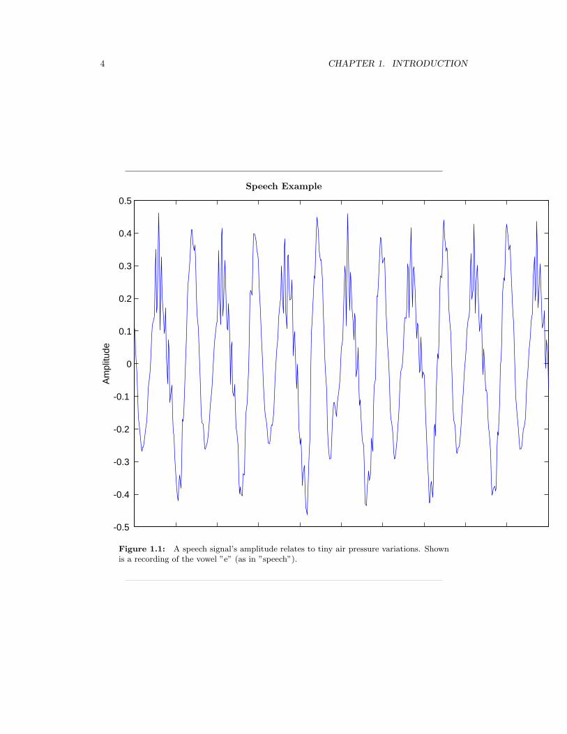
Analog signals are usually signals defined over continuous independent variable(s). Speechis produced by your vocal cords exciting acoustic resonances in your vocal tract. The resultis pressure waves propagating in the air, and the speech signal thus corresponds to a functionhaving independent variables of space and time and a value corresponding to air pressure:s (x, t) (Here we use vector notation x to denote spatial coordinates). When you recordsomeone talking, you are evaluating the speech signal at a particular spatial location, x0
say. An example of the resulting waveform s (x0, t) is shown in this figure (Figure 1.1).Photographs are static, and are continuous-valued signals defined over space. Black-
and-white images have only one value at each point in space, which amounts to its opticalreflection properties. In Figure 1.2, an image is shown, demonstrating that it (and all otherimages as well) are functions of two independent spatial variables.
Color images have values that express how reflectivity depends on the optical spectrum.Painters long ago found that mixing together combinations of the so-called primary colors–red, yellow and blue–can produce very realistic color images. Thus, images today are usuallythought of as having three values at every point in space, but a different set of colors is used:How much of red, green and blue is present. Mathematically, color pictures are multivalued–vector-valued–signals: s (x) = (r (x) , g (x) , b (x))T .
Interesting cases abound where the analog signal depends not on a continuous variable,such as time, but on a discrete variable. For example, temperature readings taken everyhour have continuous–analog–values, but the signal’s independent variable is (essentially)the integers.
1.1.2 Digital Signals
The word ”digital” means discrete-valued and implies the signal has an integer-valued inde-pendent variable. Digital information includes numbers and symbols (characters typed on
3
4 CHAPTER 1. INTRODUCTION
Speech Example
-0.5
-0.4
-0.3
-0.2
-0.1
0
0.1
0.2
0.3
0.4
0.5
Am
plitu
de
Figure 1.1: A speech signal’s amplitude relates to tiny air pressure variations. Shownis a recording of the vowel ”e” (as in ”speech”).
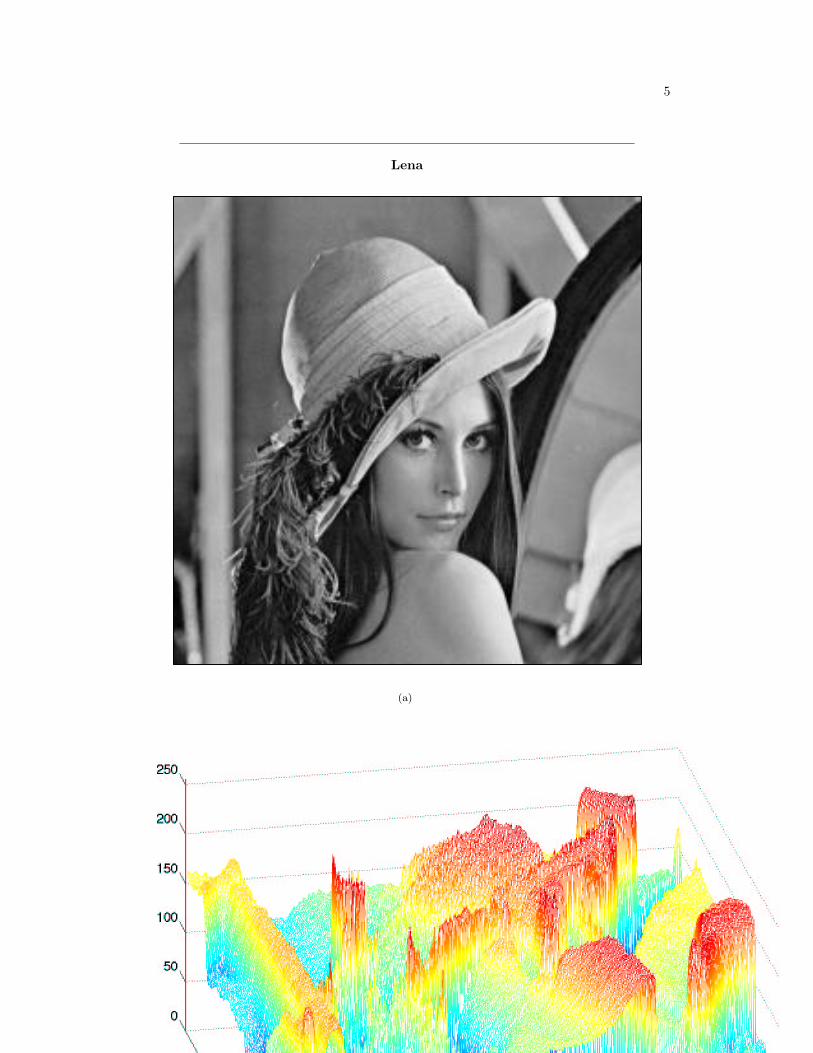
5
Lena
(a)
(b)
Figure 1.2: On the left is the classic Lena image, which is used ubiquitously as a testimage. It contains straight and curved lines, complicated texture, and a face. On theright is a perspective display of the Lena image as a signal: a function of two spatialvariables. The colors merely help show what signal values are about the same size. Inthis image, signal values range between 0 and 255; why is that?
6 CHAPTER 1. INTRODUCTION
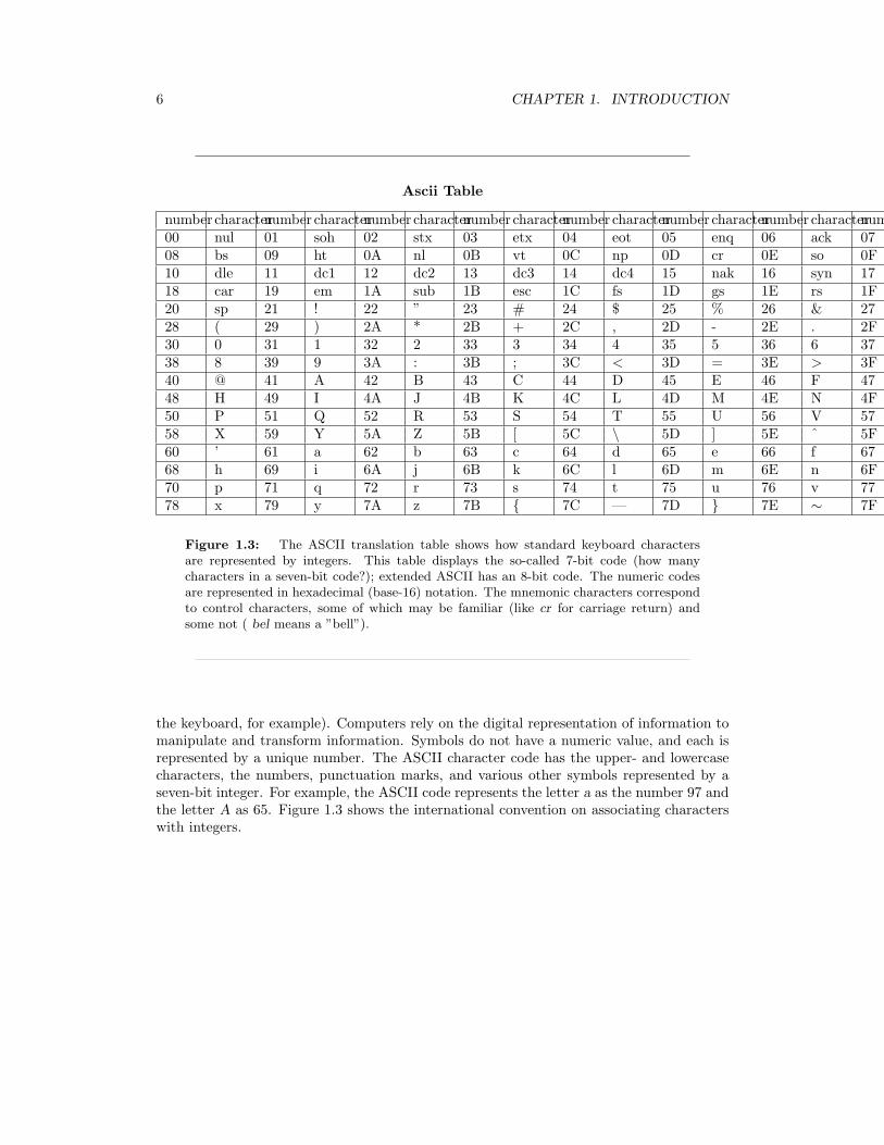
Ascii Table
number characternumber characternumber characternumber characternumber characternumber characternumber characternumber character00 nul 01 soh 02 stx 03 etx 04 eot 05 enq 06 ack 07 bel08 bs 09 ht 0A nl 0B vt 0C np 0D cr 0E so 0F si10 dle 11 dc1 12 dc2 13 dc3 14 dc4 15 nak 16 syn 17 etb18 car 19 em 1A sub 1B esc 1C fs 1D gs 1E rs 1F us20 sp 21 ! 22 ” 23 # 24 $ 25 % 26 & 27 ’28 ( 29 ) 2A * 2B + 2C , 2D - 2E . 2F /30 0 31 1 32 2 33 3 34 4 35 5 36 6 37 738 8 39 9 3A : 3B ; 3C < 3D = 3E > 3F ?40 @ 41 A 42 B 43 C 44 D 45 E 46 F 47 G48 H 49 I 4A J 4B K 4C L 4D M 4E N 4F 050 P 51 Q 52 R 53 S 54 T 55 U 56 V 57 W58 X 59 Y 5A Z 5B [ 5C \ 5D ] 5E ˆ 5F60 ’ 61 a 62 b 63 c 64 d 65 e 66 f 67 g68 h 69 i 6A j 6B k 6C l 6D m 6E n 6F o70 p 71 q 72 r 73 s 74 t 75 u 76 v 77 w78 x 79 y 7A z 7B 7C — 7D 7E ∼ 7F del
Figure 1.3: The ASCII translation table shows how standard keyboard charactersare represented by integers. This table displays the so-called 7-bit code (how manycharacters in a seven-bit code?); extended ASCII has an 8-bit code. The numeric codesare represented in hexadecimal (base-16) notation. The mnemonic characters correspondto control characters, some of which may be familiar (like cr for carriage return) andsome not ( bel means a ”bell”).
the keyboard, for example). Computers rely on the digital representation of information tomanipulate and transform information. Symbols do not have a numeric value, and each isrepresented by a unique number. The ASCII character code has the upper- and lowercasecharacters, the numbers, punctuation marks, and various other symbols represented by aseven-bit integer. For example, the ASCII code represents the letter a as the number 97 andthe letter A as 65. Figure 1.3 shows the international convention on associating characterswith integers.
Chapter 2
Signals and Systems: A FirstLook
3.1 System Classifications and Properties
2.1.1 Introduction
In this module some of the basic classifications of systems will be briefly introduced and themost important properties of these systems are explained. As can be seen, the properties ofa system provide an easy way to separate one system from another. Understanding thesebasic difference’s between systems, and their properties, will be a fundamental concept usedin all signal and system courses, such as digital signal processing (DSP). Once a set ofsystems can be identified as sharing particular properties, one no longer has to deal withproving a certain characteristic of a system each time, but it can simply be accepted do thethe systems classification. Also remember that this classification presented here is neitherexclusive (systems can belong to several different classificatins) nor is it unique (there areother methods of classification).
2.1.2 Classification of Systems
Along with the classification of systems below, it is also important to understand the Clas-sification of Signals.
2.1.2.1 Continuous vs. Discrete
This may be the simplest classification to understand as the idea of discrete-time andcontinuous-time is one of the most fundamental properties to all of signals and system.A system where the input and output signals are continuous is a continuous system , andone where the input and ouput signals are discrete is a discrete system .
2.1.2.2 Linear vs. Nonlinear
A linear system is any system that obeys the properties of scaling (homogeneity) andsuperposition (additivity), while a nonlinear system is any system that does not obey atleast one of these.
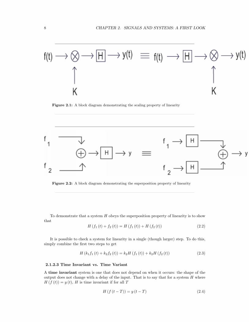
To show that a system H obeys the scaling property is to show that
H (kf (t)) = kH (f (t)) (2.1)
7
8 CHAPTER 2. SIGNALS AND SYSTEMS: A FIRST LOOK
Figure 2.1: A block diagram demonstrating the scaling property of linearity
Figure 2.2: A block diagram demonstrating the superposition property of linearity
To demonstrate that a system H obeys the superposition property of linearity is to showthat
H (f1 (t) + f2 (t)) = H (f1 (t)) +H (f2 (t)) (2.2)
It is possible to check a system for linearity in a single (though larger) step. To do this,simply combine the first two steps to get
H (k1f1 (t) + k2f2 (t)) = k2H (f1 (t)) + k2H (f2 (t)) (2.3)
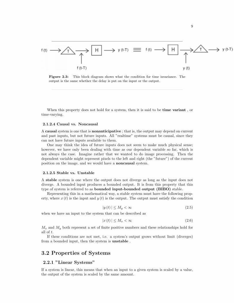
2.1.2.3 Time Invariant vs. Time Variant
A time invariant system is one that does not depend on when it occurs: the shape of theoutput does not change with a delay of the input. That is to say that for a system H whereH (f (t)) = y (t), H is time invariant if for all T
H (f (t− T )) = y (t− T ) (2.4)
9
Figure 2.3: This block diagram shows what the condition for time invariance. Theoutput is the same whether the delay is put on the input or the output.
When this property does not hold for a system, then it is said to be time variant , ortime-varying.
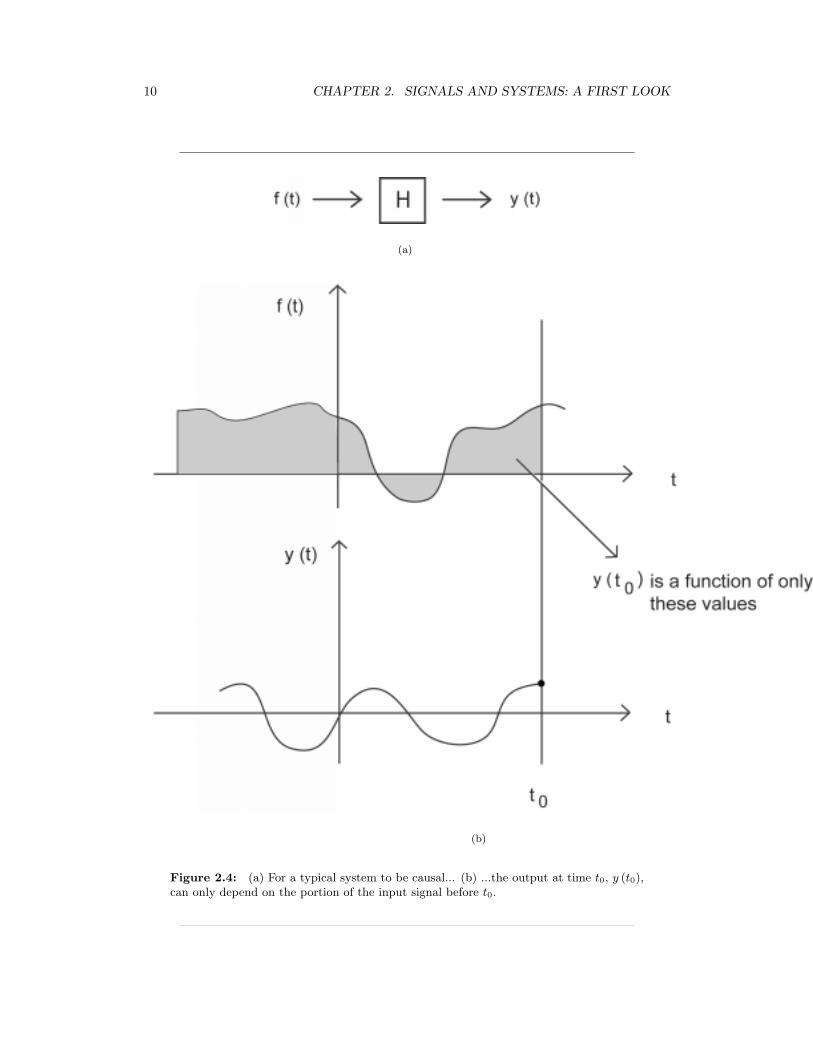
2.1.2.4 Causal vs. Noncausal
A causal system is one that is nonanticipative ; that is, the output may depend on currentand past inputs, but not future inputs. All ”realtime” systems must be causal, since theycan not have future inputs available to them.
One may think the idea of future inputs does not seem to make much physical sense;however, we have only been dealing with time as our dependent variable so far, which isnot always the case. Imagine rather that we wanted to do image processing. Then thedependent variable might represent pixels to the left and right (the ”future”) of the currentposition on the image, and we would have a noncausal system.
2.1.2.5 Stable vs. Unstable
A stable system is one where the output does not diverge as long as the input does notdiverge. A bounded input produces a bounded output. It is from this property that thistype of system is referred to as bounded input-bounded output (BIBO) stable.
Representing this in a mathematical way, a stable system must have the following prop-erty, where x (t) is the input and y (t) is the output. The output must satisfy the condition
|y (t) | ≤My <∞ (2.5)
when we have an input to the system that can be described as
|x (t) | ≤Mx <∞ (2.6)
Mx and My both represent a set of finite positive numbers and these relationships hold forall of t.
If these conditions are not met, i.e. a system’s output grows without limit (diverges)from a bounded input, then the system is unstable .
3.2 Properties of Systems
2.2.1 ”Linear Systems”
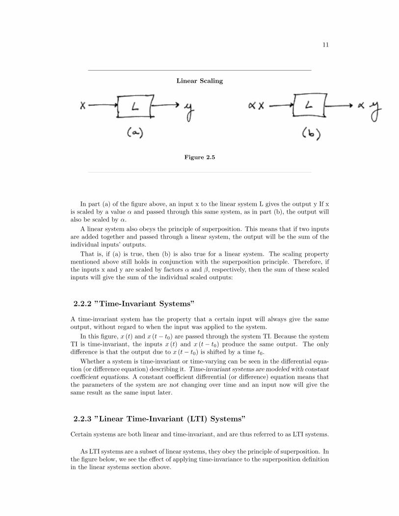
If a system is linear, this means that when an input to a given system is scaled by a value,the output of the system is scaled by the same amount.
10 CHAPTER 2. SIGNALS AND SYSTEMS: A FIRST LOOK
(a)
(b)
Figure 2.4: (a) For a typical system to be causal... (b) ...the output at time t0, y (t0),can only depend on the portion of the input signal before t0.
11
Linear Scaling
Figure 2.5
In part (a) of the figure above, an input x to the linear system L gives the output y If xis scaled by a value α and passed through this same system, as in part (b), the output willalso be scaled by α.
A linear system also obeys the principle of superposition. This means that if two inputsare added together and passed through a linear system, the output will be the sum of theindividual inputs’ outputs.
That is, if (a) is true, then (b) is also true for a linear system. The scaling propertymentioned above still holds in conjunction with the superposition principle. Therefore, ifthe inputs x and y are scaled by factors α and β, respectively, then the sum of these scaledinputs will give the sum of the individual scaled outputs:
2.2.2 ”Time-Invariant Systems”
A time-invariant system has the property that a certain input will always give the sameoutput, without regard to when the input was applied to the system.
In this figure, x (t) and x (t− t0) are passed through the system TI. Because the systemTI is time-invariant, the inputs x (t) and x (t− t0) produce the same output. The onlydifference is that the output due to x (t− t0) is shifted by a time t0.
Whether a system is time-invariant or time-varying can be seen in the differential equa-tion (or difference equation) describing it. Time-invariant systems are modeled with constantcoefficient equations. A constant coefficient differential (or difference) equation means thatthe parameters of the system are not changing over time and an input now will give thesame result as the same input later.
2.2.3 ”Linear Time-Invariant (LTI) Systems”
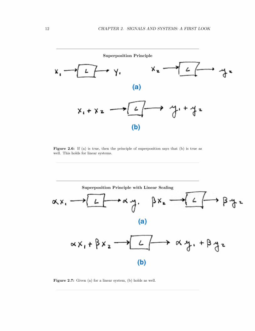
Certain systems are both linear and time-invariant, and are thus referred to as LTI systems.
As LTI systems are a subset of linear systems, they obey the principle of superposition. Inthe figure below, we see the effect of applying time-invariance to the superposition definitionin the linear systems section above.
12 CHAPTER 2. SIGNALS AND SYSTEMS: A FIRST LOOK
Superposition Principle
Figure 2.6: If (a) is true, then the principle of superposition says that (b) is true aswell. This holds for linear systems.
Superposition Principle with Linear Scaling
Figure 2.7: Given (a) for a linear system, (b) holds as well.
13
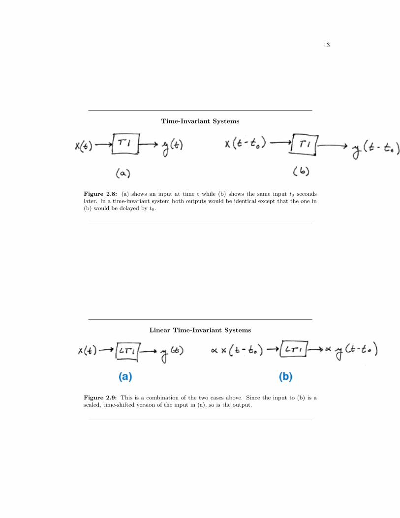
Time-Invariant Systems
Figure 2.8: (a) shows an input at time t while (b) shows the same input t0 secondslater. In a time-invariant system both outputs would be identical except that the one in(b) would be delayed by t0.
Linear Time-Invariant Systems
Figure 2.9: This is a combination of the two cases above. Since the input to (b) is ascaled, time-shifted version of the input in (a), so is the output.
14 CHAPTER 2. SIGNALS AND SYSTEMS: A FIRST LOOK
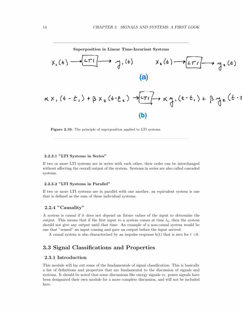
Superposition in Linear Time-Invariant Systems
Figure 2.10: The principle of superposition applied to LTI systems
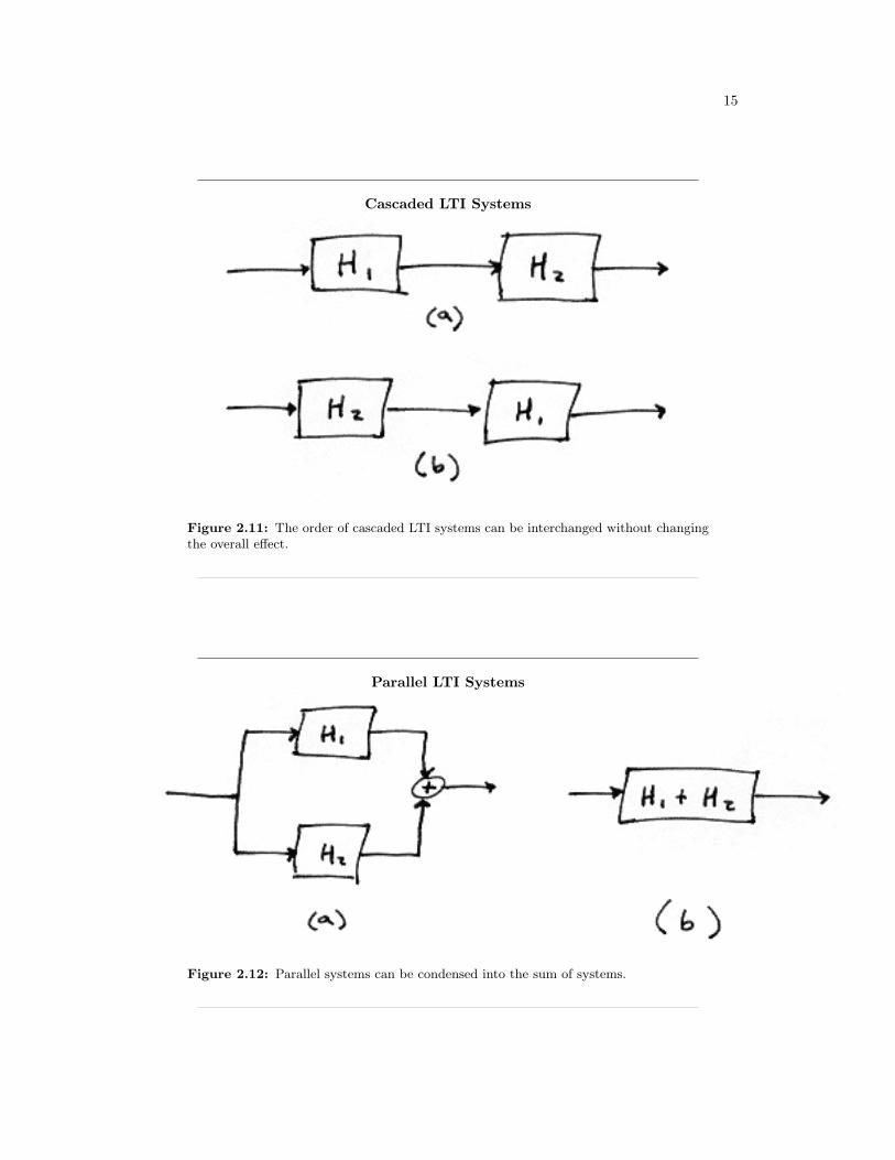
2.2.3.1 ”LTI Systems in Series”
If two or more LTI systems are in series with each other, their order can be interchangedwithout affecting the overall output of the system. Systems in series are also called cascadedsystems.
2.2.3.2 ”LTI Systems in Parallel”
If two or more LTI systems are in parallel with one another, an equivalent system is onethat is defined as the sum of these individual systems.
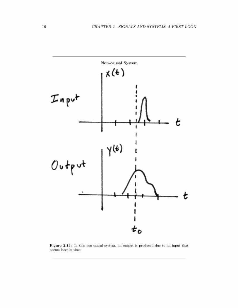
2.2.4 ”Causality”
A system is causal if it does not depend on future values of the input to determine theoutput. This means that if the first input to a system comes at time t0, then the systemshould not give any output until that time. An example of a non-causal system would beone that ”sensed” an input coming and gave an output before the input arrived:
A causal system is also characterized by an impulse response h(t) that is zero for t <0.
3.3 Signal Classifications and Properties
2.3.1 Introduction
This module will lay out some of the fundamentals of signal classification. This is basicallya list of definitions and properties that are fundamental to the discussion of signals andsystems. It should be noted that some discussions like energy signals vs. power signals havebeen designated their own module for a more complete discussion, and will not be includedhere.
15
Cascaded LTI Systems
Figure 2.11: The order of cascaded LTI systems can be interchanged without changingthe overall effect.
Parallel LTI Systems
Figure 2.12: Parallel systems can be condensed into the sum of systems.
16 CHAPTER 2. SIGNALS AND SYSTEMS: A FIRST LOOK
Non-causal System
Figure 2.13: In this non-causal system, an output is produced due to an input thatoccurs later in time.
17
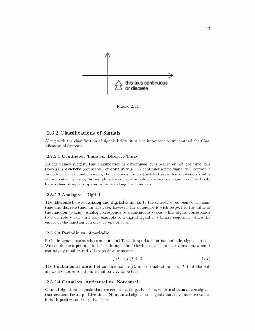
Figure 2.14
2.3.2 Classifications of Signals
Along with the classification of signals below, it is also important to understand the Clas-sification of Systems.
2.3.2.1 Continuous-Time vs. Discrete-Time
As the names suggest, this classification is determined by whether or not the time axis(x-axis) is discrete (countable) or continuous . A continuous-time signal will contain avalue for all real numbers along the time axis. In contrast to this, a discrete-time signal isoften created by using the sampling theorem to sample a continuous signal, so it will onlyhave values at equally spaced intervals along the time axis.
2.3.2.2 Analog vs. Digital
The difference between analog and digital is similar to the difference between continuous-time and discrete-time. In this case, however, the difference is with respect to the value ofthe function (y-axis). Analog corresponds to a continuous y-axis, while digital correspondsto a discrete y-axis. An easy example of a digital signal is a binary sequence, where thevalues of the function can only be one or zero.
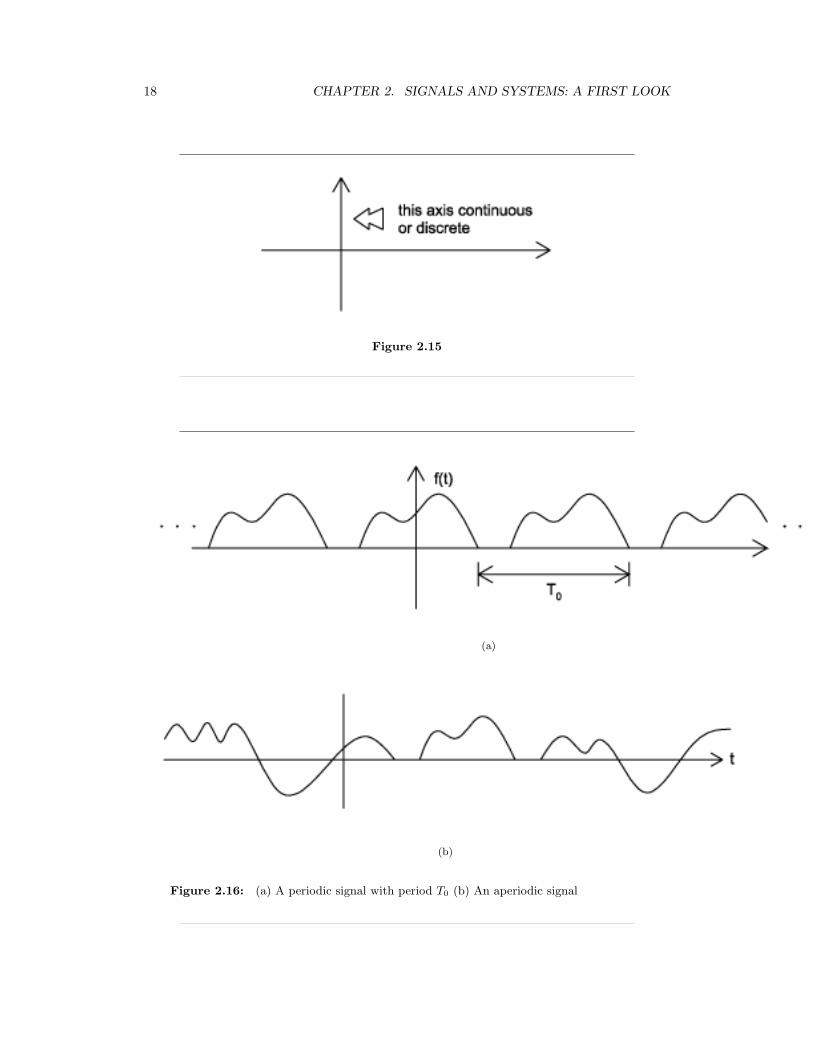
2.3.2.3 Periodic vs. Aperiodic
Periodic signals repeat with some period T, while aperiodic, or nonperiodic, signals do not.We can define a periodic function through the following mathematical expression, where tcan be any number and T is a positive constant:
f (t) = f (T + t) (2.7)
The fundamental period of our function, f (t), is the smallest value of T that the stillallows the above equation, Equation 2.7, to be true.
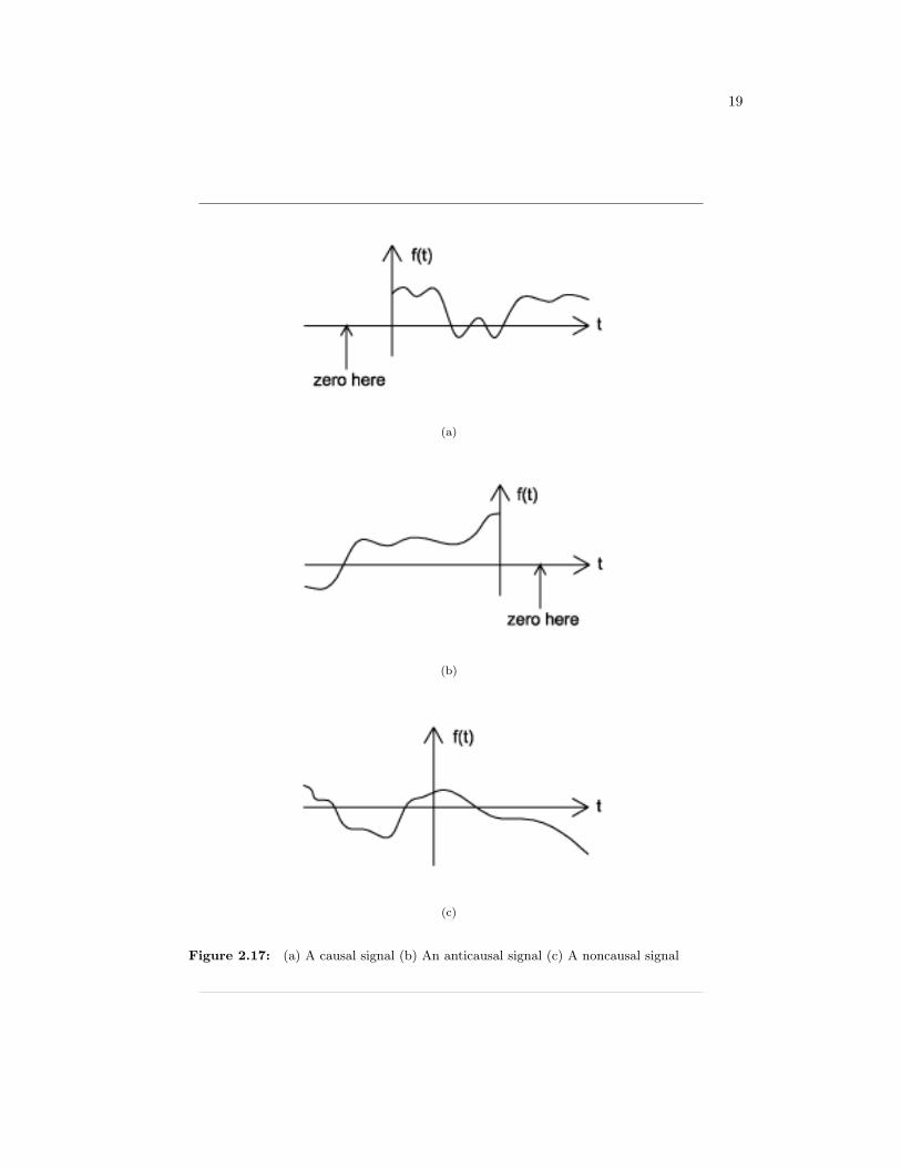
2.3.2.4 Causal vs. Anticausal vs. Noncausal
Causal signals are signals that are zero for all negative time, while anitcausal are signalsthat are zero for all positive time. Noncausal signals are signals that have nonzero valuesin both positive and negative time.
18 CHAPTER 2. SIGNALS AND SYSTEMS: A FIRST LOOK
Figure 2.15
(a)
(b)
Figure 2.16: (a) A periodic signal with period T0 (b) An aperiodic signal
19
(a)
(b)
(c)
Figure 2.17: (a) A causal signal (b) An anticausal signal (c) A noncausal signal
20 CHAPTER 2. SIGNALS AND SYSTEMS: A FIRST LOOK
(a)
(b)
Figure 2.18: (a) An even signal (b) An odd signal
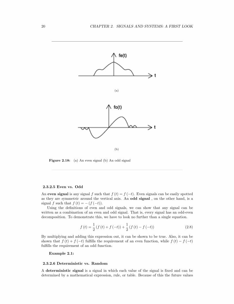
2.3.2.5 Even vs. Odd
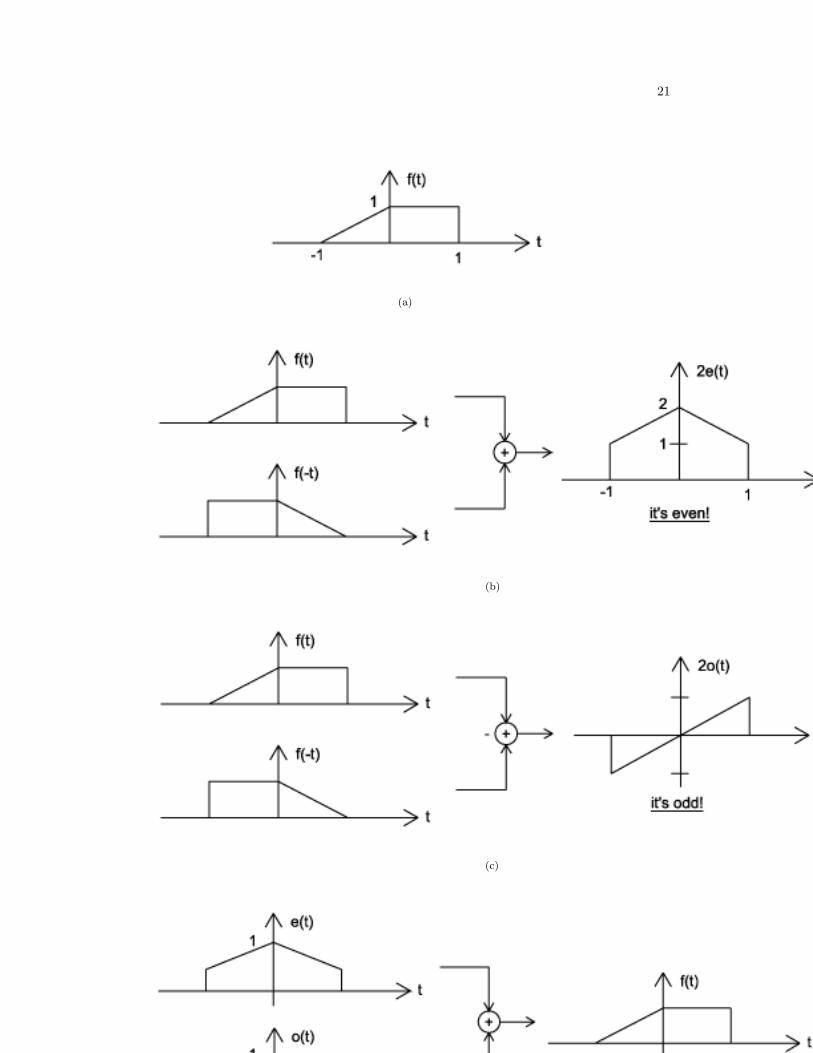
An even signal is any signal f such that f (t) = f (−t). Even signals can be easily spottedas they are symmetric around the vertical axis. An odd signal , on the other hand, is asignal f such that f (t) = − (f (−t)).
Using the definitions of even and odd signals, we can show that any signal can bewritten as a combination of an even and odd signal. That is, every signal has an odd-evendecomposition. To demonstrate this, we have to look no further than a single equation.
f (t) =12
(f (t) + f (−t)) +12
(f (t)− f (−t)) (2.8)
By multiplying and adding this expression out, it can be shown to be true. Also, it can beshown that f (t) + f (−t) fulfills the requirement of an even function, while f (t) − f (−t)fulfills the requirement of an odd function.
Example 2.1:
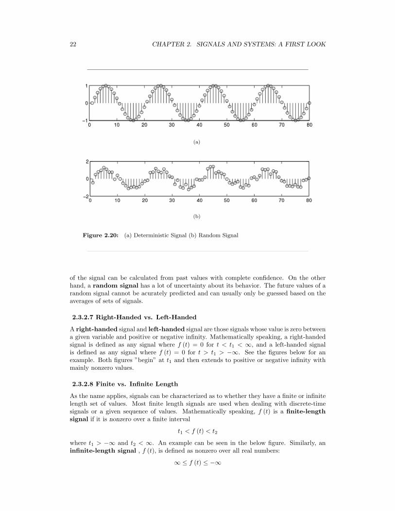
2.3.2.6 Deterministic vs. Random
A deterministic signal is a signal in which each value of the signal is fixed and can bedetermined by a mathematical expression, rule, or table. Because of this the future values
21
(a)
(b)
(c)
(d)
Figure 2.19: (a) The signal we will decompose using odd-even decomposition (b)Even part: e (t) = 1
2(f (t) + f (−t)) (c) Odd part: o (t) = 1
2(f (t)− f (−t)) (d) Check:
e (t) + o (t) = f (t)
22 CHAPTER 2. SIGNALS AND SYSTEMS: A FIRST LOOK
(a)
(b)
Figure 2.20: (a) Deterministic Signal (b) Random Signal
of the signal can be calculated from past values with complete confidence. On the otherhand, a random signal has a lot of uncertainty about its behavior. The future values of arandom signal cannot be acurately predicted and can usually only be guessed based on theaverages of sets of signals.
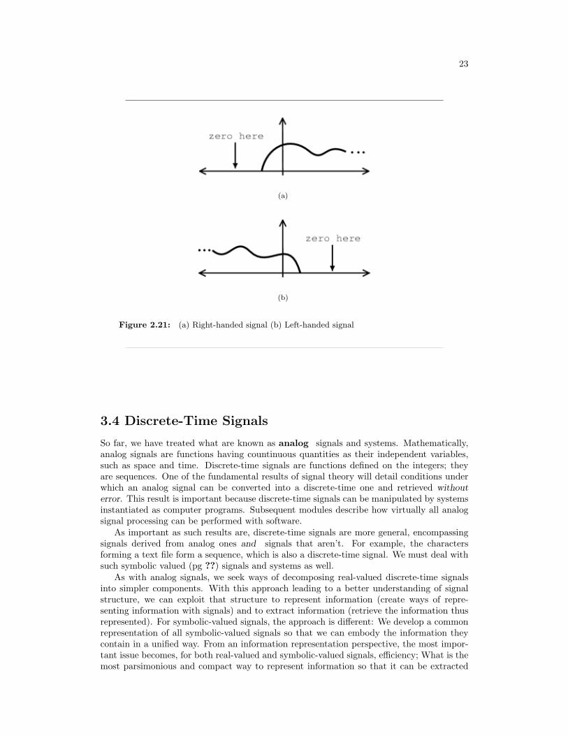
2.3.2.7 Right-Handed vs. Left-Handed
A right-handed signal and left-handed signal are those signals whose value is zero betweena given variable and positive or negative infinity. Mathematically speaking, a right-handedsignal is defined as any signal where f (t) = 0 for t < t1 < ∞, and a left-handed signalis defined as any signal where f (t) = 0 for t > t1 > −∞. See the figures below for anexample. Both figures ”begin” at t1 and then extends to positive or negative infinity withmainly nonzero values.
2.3.2.8 Finite vs. Infinite Length
As the name applies, signals can be characterized as to whether they have a finite or infinitelength set of values. Most finite length signals are used when dealing with discrete-timesignals or a given sequence of values. Mathematically speaking, f (t) is a finite-lengthsignal if it is nonzero over a finite interval
t1 < f (t) < t2
where t1 > −∞ and t2 < ∞. An example can be seen in the below figure. Similarly, aninfinite-length signal , f (t), is defined as nonzero over all real numbers:
∞ ≤ f (t) ≤ −∞
23
(a)
(b)
Figure 2.21: (a) Right-handed signal (b) Left-handed signal
3.4 Discrete-Time Signals
So far, we have treated what are known as analog signals and systems. Mathematically,analog signals are functions having countinuous quantities as their independent variables,such as space and time. Discrete-time signals are functions defined on the integers; theyare sequences. One of the fundamental results of signal theory will detail conditions underwhich an analog signal can be converted into a discrete-time one and retrieved withouterror. This result is important because discrete-time signals can be manipulated by systemsinstantiated as computer programs. Subsequent modules describe how virtually all analogsignal processing can be performed with software.
As important as such results are, discrete-time signals are more general, encompassingsignals derived from analog ones and signals that aren’t. For example, the charactersforming a text file form a sequence, which is also a discrete-time signal. We must deal withsuch symbolic valued (pg ??) signals and systems as well.
As with analog signals, we seek ways of decomposing real-valued discrete-time signalsinto simpler components. With this approach leading to a better understanding of signalstructure, we can exploit that structure to represent information (create ways of repre-senting information with signals) and to extract information (retrieve the information thusrepresented). For symbolic-valued signals, the approach is different: We develop a commonrepresentation of all symbolic-valued signals so that we can embody the information theycontain in a unified way. From an information representation perspective, the most impor-tant issue becomes, for both real-valued and symbolic-valued signals, efficiency; What is themost parsimonious and compact way to represent information so that it can be extracted
24 CHAPTER 2. SIGNALS AND SYSTEMS: A FIRST LOOK
Figure 2.22: Finite-Length Signal. Note that it only has nonzero values on a set, finiteinterval.
later.
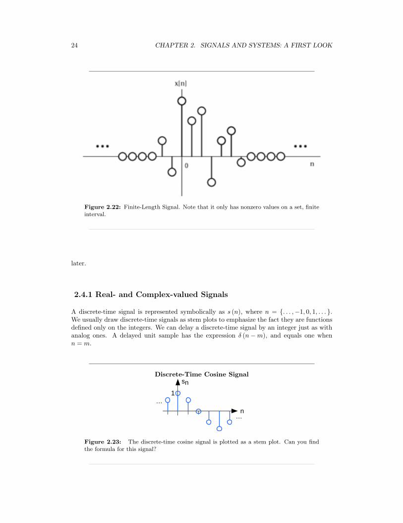
2.4.1 Real- and Complex-valued Signals
A discrete-time signal is represented symbolically as s (n), where n = . . . ,−1, 0, 1, . . . .We usually draw discrete-time signals as stem plots to emphasize the fact they are functionsdefined only on the integers. We can delay a discrete-time signal by an integer just as withanalog ones. A delayed unit sample has the expression δ (n−m), and equals one whenn = m.
Discrete-Time Cosine Signal
n
sn
1…
…
Figure 2.23: The discrete-time cosine signal is plotted as a stem plot. Can you findthe formula for this signal?
25
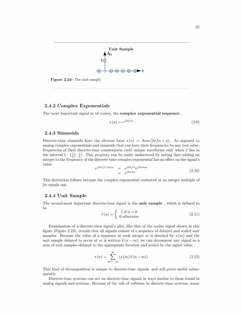
Unit Sample
1
n
δn
Figure 2.24: The unit sample.
2.4.2 Complex Exponentials
The most important signal is, of course, the complex exponential sequence .
s (n) = ej2πfn (2.9)
2.4.3 Sinusoids
Discrete-time sinusoids have the obvious form s (n) = Acos (2πfn+ φ). As opposed toanalog complex exponentials and sinusoids that can have their frequencies be any real value,frequencies of their discrete-time counterparts yield unique waveforms only when f lies inthe interval
(−(
12
), 1
2
]. This property can be easily understood by noting that adding an
integer to the frequency of the discrete-time complex exponential has no effect on the signal’svalue.
ej2π(f+m)n = ej2πfnej2πmn
= ej2πfn (2.10)
This derivation follows because the complex exponential evaluated at an integer multiple of2π equals one.
2.4.4 Unit Sample
The second-most important discrete-time signal is the unit sample , which is defined tobe
δ (n) =
1 if n = 00 otherwise (2.11)
Examination of a discrete-time signal’s plot, like that of the cosine signal shown in thisfigure (Figure 2.23), reveals that all signals consist of a sequence of delayed and scaled unitsamples. Because the value of a sequence at each integer m is denoted by s (m) and theunit sample delayed to occur at m is written δ (n−m), we can decompose any signal as asum of unit samples delayed to the appropriate location and scaled by the signal value.
s (n) =∞∑
m=−∞(s (m) δ (n−m)) (2.12)
This kind of decomposition is unique to discrete-time signals, and will prove useful subse-quently.
Discrete-time systems can act on discrete-time signals in ways similar to those found inanalog signals and systems. Because of the role of software in discrete-time systems, many

26 CHAPTER 2. SIGNALS AND SYSTEMS: A FIRST LOOK
more different systems can be envisioned and “constructed” with programs than can bewith analog signals. In fact, a special class of analog signals can be converted into discrete-time signals, processed with software, and converted back into an analog signal, all withoutthe incursion of error. For such signals, systems can be easily produced in software, withequivalent analog realizations difficult, if not impossible, to design.
2.4.5 Symbolic-valued Signals
Another interesting aspect of discrete-time signals is that their values do not need to bereal numbers. We do have real-valued discrete-time signals like the sinusoid, but we alsohave signals that denote the sequence of characters typed on the keyboard. Such characterscertainly aren’t real numbers, and as a collection of possible signal values, they have littlemathematical structure other than that they are members of a set. More formally, eachelement of the symbolic-valued signal s (n) takes on one of the values a1, . . . , aK whichcomprise the alphabet A. This technical terminology does not mean we restrict symbolsto being members of the English or Greek alphabet. They could represent keyboard char-acters, bytes (8-bit quantities), integers that convey daily temperature. Whether controlledby software or not, discrete-time systems are ultimately constructed from digital circuits,which consist entirely of analog circuit elements. Furthermore, the transmission and recep-tion of discrete-time signals, like e-mail, is accomplished with analog signals and systems.Understanding how discrete-time and analog signals and systems intertwine is perhaps themain goal of this course.
3.5 Useful Signals
Before looking at this module, hopefully you have some basic idea of what a signal is andwhat basic classifications and properties a signal can have. To review, a signal is merely afunction defined with respect to an independent variable. This variable is often time butcould represent an index of a sequence or any number of things in any number of dimensions.Most, if not all, signals that you will encounter in your studies and the real world will beable to be created from the basic signals we discuss below. Because of this, these elementarysignals are often referred to as the building blocks for all other signals.
2.5.1 Sinusoids
Probably the most important elemental signal that you will deal with is the real-valuedsinusoid. In its continuous-time form, we write the general form as
x (t) = Acos (ωt+ φ) (2.13)
where A is the amplitude, ω is the frequency, and φ represents the phase. Note that it iscommon to see ωt replaced with 2πft. Since sinusoidal signals are periodic, we can expressthe period of these, or any periodic signal, as
T =2πω
(2.14)
2.5.2 Complex Exponential Function
Maybe as important as the general sinusoid, the complex exponential function will be-come a critical part of your study of signals and systems. Its general form is written as
27
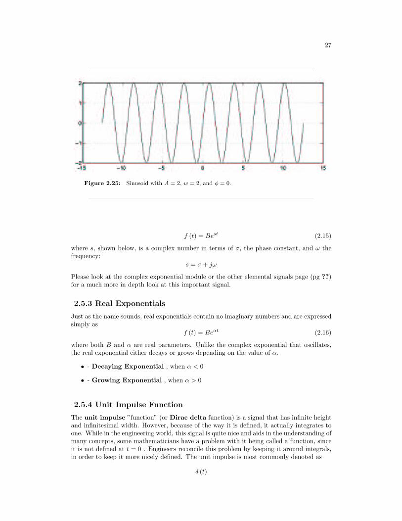
Figure 2.25: Sinusoid with A = 2, w = 2, and φ = 0.
f (t) = Best (2.15)
where s, shown below, is a complex number in terms of σ, the phase constant, and ω thefrequency:
s = σ + jω
Please look at the complex exponential module or the other elemental signals page (pg ??)for a much more in depth look at this important signal.
2.5.3 Real Exponentials
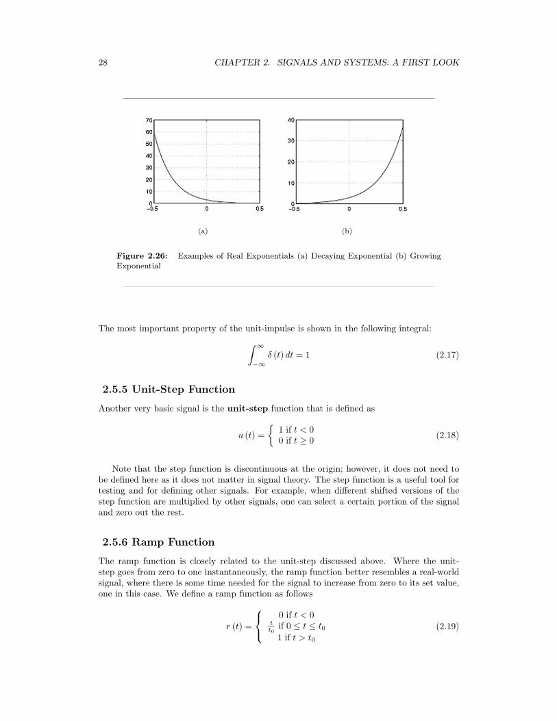
Just as the name sounds, real exponentials contain no imaginary numbers and are expressedsimply as
f (t) = Beαt (2.16)
where both B and α are real parameters. Unlike the complex exponential that oscillates,the real exponential either decays or grows depending on the value of α.
• - Decaying Exponential , when α < 0
• - Growing Exponential , when α > 0
2.5.4 Unit Impulse Function
The unit impulse ”function” (or Dirac delta function) is a signal that has infinite heightand infinitesimal width. However, because of the way it is defined, it actually integrates toone. While in the engineering world, this signal is quite nice and aids in the understanding ofmany concepts, some mathematicians have a problem with it being called a function, sinceit is not defined at t = 0 . Engineers reconcile this problem by keeping it around integrals,in order to keep it more nicely defined. The unit impulse is most commonly denoted as
δ (t)
28 CHAPTER 2. SIGNALS AND SYSTEMS: A FIRST LOOK
(a) (b)
Figure 2.26: Examples of Real Exponentials (a) Decaying Exponential (b) GrowingExponential
The most important property of the unit-impulse is shown in the following integral:∫ ∞
−∞δ (t) dt = 1 (2.17)
2.5.5 Unit-Step Function
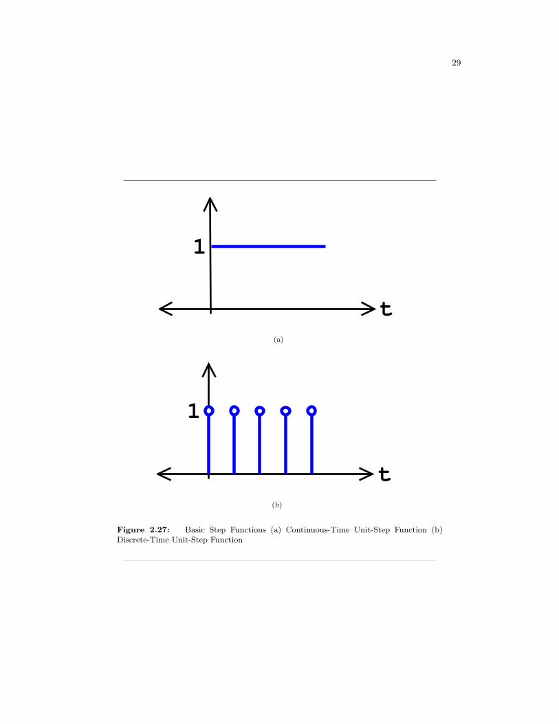
Another very basic signal is the unit-step function that is defined as
u (t) =
1 if t < 00 if t ≥ 0 (2.18)
Note that the step function is discontinuous at the origin; however, it does not need tobe defined here as it does not matter in signal theory. The step function is a useful tool fortesting and for defining other signals. For example, when different shifted versions of thestep function are multiplied by other signals, one can select a certain portion of the signaland zero out the rest.
2.5.6 Ramp Function
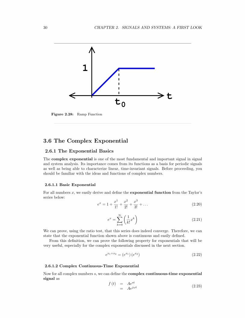
The ramp function is closely related to the unit-step discussed above. Where the unit-step goes from zero to one instantaneously, the ramp function better resembles a real-worldsignal, where there is some time needed for the signal to increase from zero to its set value,one in this case. We define a ramp function as follows
r (t) =
0 if t < 0
tt0
if 0 ≤ t ≤ t01 if t > t0
(2.19)
29
t
1
(a)
t
1
(b)
Figure 2.27: Basic Step Functions (a) Continuous-Time Unit-Step Function (b)Discrete-Time Unit-Step Function
30 CHAPTER 2. SIGNALS AND SYSTEMS: A FIRST LOOK
t
1
t0Figure 2.28: Ramp Function
3.6 The Complex Exponential
2.6.1 The Exponential Basics
The complex exponential is one of the most fundamental and important signal in signaland system analysis. Its importance comes from its functions as a basis for periodic signalsas well as being able to characterize linear, time-invariant signals. Before proceeding, youshould be familiar with the ideas and functions of complex numbers.
2.6.1.1 Basic Exponential
For all numbers x, we easily derive and define the exponential function from the Taylor’sseries below:
ex = 1 +x1
1!+x2
2!+x3
3!+ . . . (2.20)
ex =∞∑
k=0
(1k!xk
)(2.21)
We can prove, using the ratio test, that this series does indeed converge. Therefore, we canstate that the exponential function shown above is continuous and easily defined.
From this definition, we can prove the following property for exponentials that will bevery useful, especially for the complex exponentials discussed in the next section.
ex1+x2 = (ex1) (ex2) (2.22)
2.6.1.2 Complex Continuous-Time Exponential
Now for all complex numbers s, we can define the complex continuous-time exponentialsignal as
f (t) = Aest
= Aejωt (2.23)
31
where A is a constant, t is our independent variable for time, and for s imaginary, s = jω.Finally, from this equation we can reveal the ever important Euler’s Identity (for moreinformation on Euler read this short biography1):
Aejωt = Acos (ωt) + j (Asin (ωt)) (2.24)
From Euler’s Identity we can easily break the signal down into its real and imaginarycomponents. Also we can see how exponentials can be combined to represet any real signal.By modifying their frequency and phase, we can represent any signal through a superposityof many signals - all capable of being represented by an exponential.
The above expressions do not include any information on phase however. We can furthergeneralize our above expressions for the exponential to generalize sinusoids with any phaseby making a final substitution for s, s = σ + jω, which leads us to
f (t) = Aest
= Ae(σ+jω)t
= Aeσtejωt(2.25)
where we define S as the complex amplitude , or phasor , from the first two terms ofthe above equation as
S = Aeσt (2.26)
Going back to Euler’s Identity, we can rewrite the exponentials as sinusoids, where the phaseterm becomes much more apparent.
f (t) = Aeσt (cos (ωt) + jsin (ωt))= Acos (σ + ωt) + jAsin (σ + ωt) (2.27)
As stated above we can easily break this formula into its real and imaginary part as follows:
Re (f (t)) = Aeσtcos (ωt) (2.28)
Im (f (t)) = Aeσtsin (ωt) (2.29)
2.6.1.3 Complex Discrete-Time Exponential
Finally we have reached the last form of the exponential signal that we will be interestedin, the discrete-time exponential signal , which we will not give as much detail aboutas we did for its continuous-time counterpart, because they both follow the same propertiesand logic discussed above. Because it is discrete, there is only a slightly different notationused to represents its discrete nature
f [n] = BesnT
= BejωnT (2.30)
where nT represents the discrete-time instants of our signal.
2.6.2 Euler’s Relation
Along with Euler’s Identity, Euler also described a way to represent a complex exponentialsignal in terms of its real and imaginary parts through Euler’s Relation :
cos (ωt) =ejwt + e−(jwt)
2(2.31)
1http://www-groups.dcs.st-and.ac.uk/∼history/Mathematicians/Euler.html
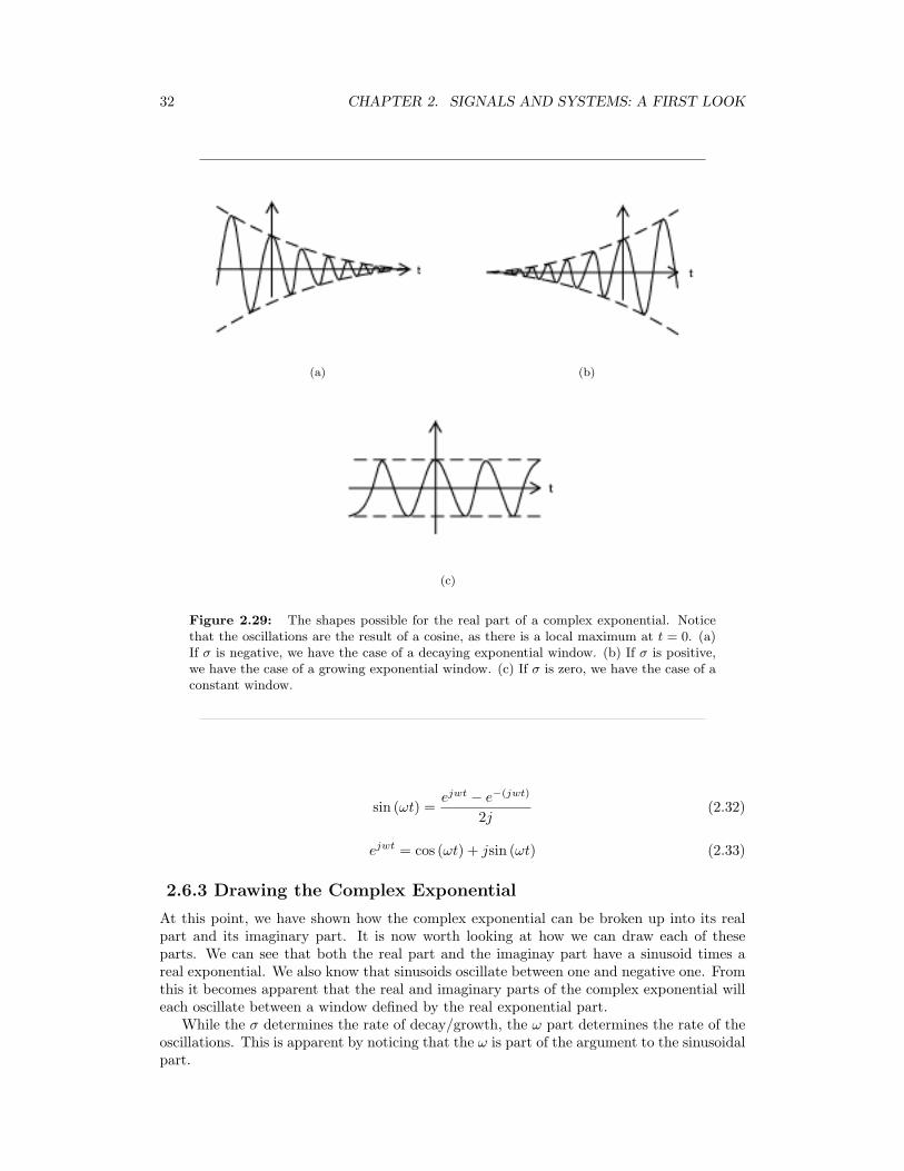
32 CHAPTER 2. SIGNALS AND SYSTEMS: A FIRST LOOK
(a) (b)
(c)
Figure 2.29: The shapes possible for the real part of a complex exponential. Noticethat the oscillations are the result of a cosine, as there is a local maximum at t = 0. (a)If σ is negative, we have the case of a decaying exponential window. (b) If σ is positive,we have the case of a growing exponential window. (c) If σ is zero, we have the case of aconstant window.
sin (ωt) =ejwt − e−(jwt)
2j(2.32)
ejwt = cos (ωt) + jsin (ωt) (2.33)
2.6.3 Drawing the Complex Exponential
At this point, we have shown how the complex exponential can be broken up into its realpart and its imaginary part. It is now worth looking at how we can draw each of theseparts. We can see that both the real part and the imaginay part have a sinusoid times areal exponential. We also know that sinusoids oscillate between one and negative one. Fromthis it becomes apparent that the real and imaginary parts of the complex exponential willeach oscillate between a window defined by the real exponential part.
While the σ determines the rate of decay/growth, the ω part determines the rate of theoscillations. This is apparent by noticing that the ω is part of the argument to the sinusoidalpart.
33
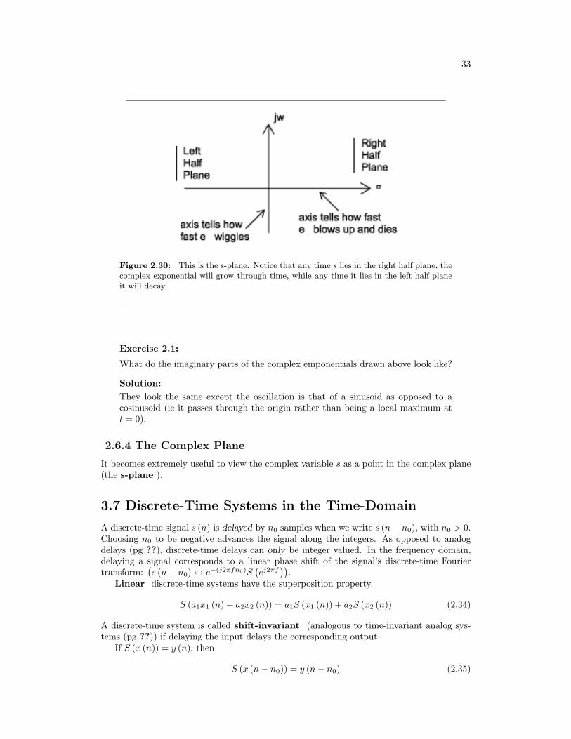
Figure 2.30: This is the s-plane. Notice that any time s lies in the right half plane, thecomplex exponential will grow through time, while any time it lies in the left half planeit will decay.
Exercise 2.1:
What do the imaginary parts of the complex emponentials drawn above look like?
Solution:They look the same except the oscillation is that of a sinusoid as opposed to acosinusoid (ie it passes through the origin rather than being a local maximum att = 0).
2.6.4 The Complex Plane
It becomes extremely useful to view the complex variable s as a point in the complex plane(the s-plane ).
3.7 Discrete-Time Systems in the Time-Domain
A discrete-time signal s (n) is delayed by n0 samples when we write s (n− n0), with n0 > 0.Choosing n0 to be negative advances the signal along the integers. As opposed to analogdelays (pg ??), discrete-time delays can only be integer valued. In the frequency domain,delaying a signal corresponds to a linear phase shift of the signal’s discrete-time Fouriertransform:
(s (n− n0) ↔ e−(j2πfn0)S
(ej2πf
)).
Linear discrete-time systems have the superposition property.
S (a1x1 (n) + a2x2 (n)) = a1S (x1 (n)) + a2S (x2 (n)) (2.34)
A discrete-time system is called shift-invariant (analogous to time-invariant analog sys-tems (pg ??)) if delaying the input delays the corresponding output.
If S (x (n)) = y (n), then
S (x (n− n0)) = y (n− n0) (2.35)
34 CHAPTER 2. SIGNALS AND SYSTEMS: A FIRST LOOK
We use the term shift-invariant to emphasize that delays can only have integer values indiscrete-time, while in analog signals, delays can be arbitrarily valued.
We want to concentrate on systems that are both linear and shift-invariant. It willbe these that allow us the full power of frequency-domain analysis and implementations.Because we have no physical constraints in ”constructing” such systems, we need only amathematical specification. In analog systems, the differential equation specifies the input-output relationship in the time-domain. The corresponding discrete-time specification isthe difference equation .
y (n) = a1y (n− 1) + · · ·+ apy (n− p) + b0x (n) + b1x (n− 1) + · · ·+ bqx (n− q) (2.36)
Here, the output signal y (n) is related to its past values y (n− l), l = 1, . . . , p, andto the current and past values of the input signal x (n). The system’s characteristics aredetermined by the choices for the number of coefficients p and q and the coefficients’ valuesa1, . . . , ap and b0, b1, . . . , bq.
aside: There is an asymmetry in the coefficients: where is a0? This coefficientwould multiply the y(n) term in Equation 2.36. We have essentially divided theequation by it, which does not change the input-output relationship. We have thuscreated the convention that a0 is always one.
As opposed to differential equations, which only provide an implicit description of asystem (we must somehow solve the differential equation), difference equations provide anexplicit way of computing the output for any input. We simply express the differenceequation by a program that calculates each output from the previous output values, andthe current and previous inputs.
Difference equations are usually expressed in software with for loops. A MATLABprogram that would compute the first 1000 values of the output has the form
for n=1:1000y(n) = sum(a.*y(n-1:-1:n-p)) + sum(b.*x(n:-1:n-q));end
An important detail emerges when we consider making this program work; in fact, aswritten it has (at least) two bugs. What input and output values enter into the computationof y(1)? We need values for y(0), y(-1), ..., values we have not yet computed. To computethem, we would need more previous values of the output, which we have not yet computed.To compute these values, we would need even earlier values, ad infinitum. The way outof this predicament is to specify the system’s initial conditions : we must provide the poutput values that occurred before the input started. These values can be arbitrary, butthe choice does impact how the system responds to a given input. One choice gives rise to alinear system: Make the initial conditions zero. The reason lies in the definition of a linearsystem: The only way that the output to a sum of signals can be the sum of the individualoutputs occurs when the initial conditions in each case are zero.
Exercise 2.2:
The initial condition issue resolves making sense of the difference equation forinputs that start at some index. However, the program will not work because of aprogramming, not conceptual, error. What is it? How can it be ”fixed?”
Solution:The indices can be negative, and this condition is not allowed in MATLAB. To fixit, we must start the signals later in the array.
35
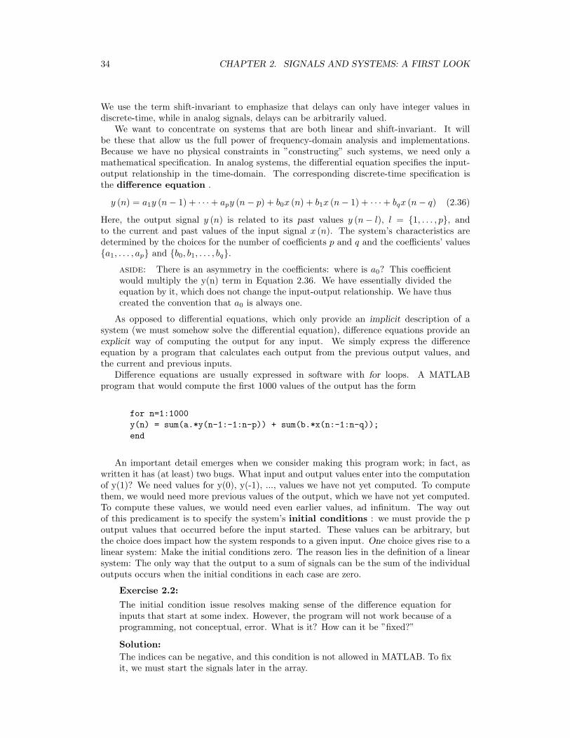
Table 1n x(n) y(n)-1 0 00 1 b1 0 ba2 0 ba2
: 0 :n 0 ban
Figure 2.31
Example 2.2:
Let’s consider the simple system having p = 1 and q = 0.
y (n) = ay (n− 1) + bx (n) (2.37)
To compute the output at some index, this difference equation says we need to knowwhat the previous output y (n− 1) and what the input signal is at that momentof time. In more detail, let’s compute this system’s output to a unit-sample input:x (n) = δ (n). Because the input is zero for negative indices, we start by trying tocompute the output at n = 0.
y (0) = ay (−1) + b (2.38)
What is the value of y (−1)? Because we have used an input that is zero for allnegative indices, it is reasonable to assume that the output is also zero. Certainly,the difference equation would not describe a linear system if the input that is zerofor all time did not produce a zero output. With this assumption, y (−1) = 0,leaving y (0) = b. For n > 0, the input unit-sample is zero, which leaves us withthe difference equation ∀n, n > 0 : y (n) = ay (n− 1). We can envision how thefilter responds to this input by making a table.
y (n) = ay (n− 1) + bδ (n) (2.39)
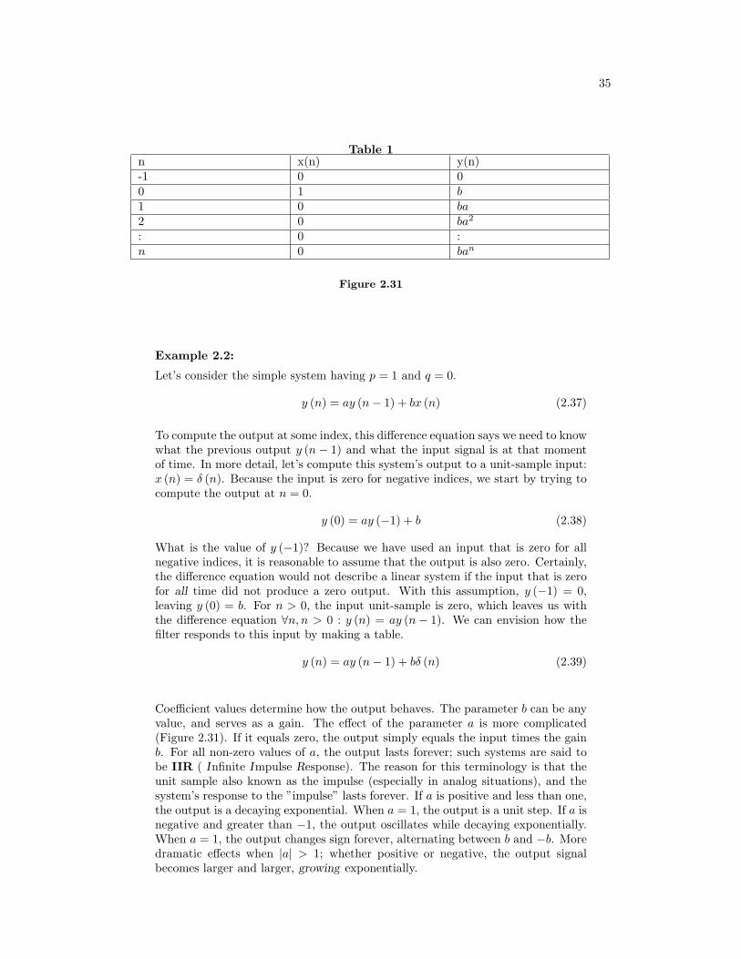
Coefficient values determine how the output behaves. The parameter b can be anyvalue, and serves as a gain. The effect of the parameter a is more complicated(Figure 2.31). If it equals zero, the output simply equals the input times the gainb. For all non-zero values of a, the output lasts forever; such systems are said tobe IIR ( Infinite Impulse Response). The reason for this terminology is that theunit sample also known as the impulse (especially in analog situations), and thesystem’s response to the ”impulse” lasts forever. If a is positive and less than one,the output is a decaying exponential. When a = 1, the output is a unit step. If a isnegative and greater than −1, the output oscillates while decaying exponentially.When a = 1, the output changes sign forever, alternating between b and −b. Moredramatic effects when |a| > 1; whether positive or negative, the output signalbecomes larger and larger, growing exponentially.
36 CHAPTER 2. SIGNALS AND SYSTEMS: A FIRST LOOK
1
n
y(n)a = 0.5, b = 1
n
-1
1y(n)a = –0.5, b = 1
n0
2
4y(n)a = 1.1, b = 1
x(n)
n
n
Figure 2.32: The input to the simple example system, a unit sample, is shown at thetop, with the outputs for several system parameter values shown below.
Positive values of a are used in population models to describe how population sizeincreases over time. Here, n might correspond to generation. The difference equa-tion says that the number in the next generation is some multiple of the previousone. If this multiple is less than one, the population becomes extinct; if greaterthan one, the population flourishes. The same difference equation also describesthe effect of compound interest on deposits. Here, n indexes the times at whichcompounding occurs (daily, monthly, etc.), a equals the compound interest rateplusone, and b = 1 (the bank provides no gain). In signal processing applications,we typically require that the output remain bounded for any input. For our ex-ample, that means that we restrict |a| = 1 and chose values for it and the gainaccording to the application.
Exercise 2.3:
Note that the difference equation (Equation 2.36),
y (n) = a1y (n− 1) + · · ·+ apy (n− p) + b0x (n) + b1x (n− 1) + · · ·+ bqx (n− q)
does not involve terms like y (n+ 1) or x (n+ 1) on the equation’s right side. Cansuch terms also be included? Why or why not?
Solution:Such terms would require the system to know what future input or output valueswould be before the current value was computed. Thus, such terms can causedifficulties.
Example 2.3:
A somewhat different system has no ”a” coefficients. Consider the difference equa-tion
y (n) =1q
(x (n) + · · ·+ x (n− q + 1)) (2.40)
Because this system’s output depends only on current and previous input values, weneed not be concerned with initial conditions. When the input is a unit-sample,
37
y(n)
n
15
Figure 2.33: The plot shows the unit-sample response of a length-5 boxcar filter.
the output equals 1q for n = 0, . . . , q − 1, then equals zero thereafter. Such
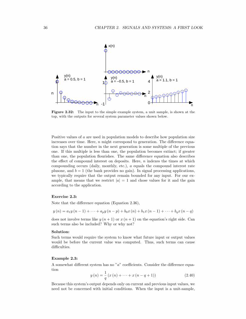
systems are said to be FIR ( Finite Impulse Response) because their unit sampleresponses have finite duration. Plotting this response (Figure 2.33) shows that theunit-sample response is a pulse of width q and height 1
q . This waveform is alsoknown as a boxcar, hence the name boxcar filter given to this system. (We’llderive its frequency response and develop its filtering interpretation in the nextsection.) For now, note that the difference equation says that each output valueequals the average of the input’s current and previous values. Thus, the outputequals the running average of input’s previous q values. Such a system could beused to produce the average weekly temperature (q = 7) that could be updateddaily.
3.8 The Impulse Function
In engineering, we often deal with the idea of an action occuring at a point. Whetherit be a force at a point in space or a signal at a point in time, it becomes worth while todevelop some way of quantitatively defining this. This leads us to the idea of a unit impulse,probably the second most important function, next to the complex exponential, in systemsand signals course.
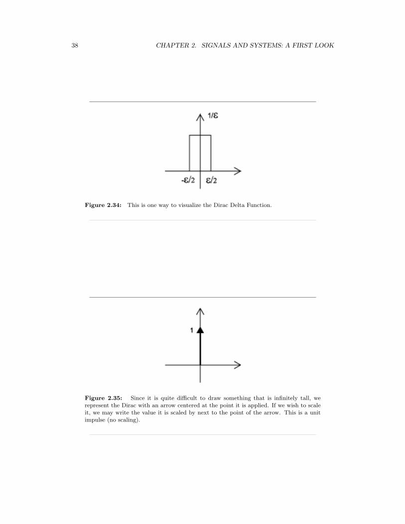
2.8.1 Dirac Delta Function
The Dirac Delta function , often referred to as the unit impulse or delta function, is thefunction that defines the idea of a unit impulse. This function is one that is infinitesimallynarrow, infinitely tall, yet integrates to unity , one (see Equation 2.41 below). Perhaps thesimplest way to visualize this is as a rectangular pulse from a− ε
2 to a+ ε2 with a height of
1ε . As we take the limit of this, lim
ε→00, we see that the width tends to zero and the height
tends to infinity as the total area remains constant at one. The impulse function is oftenwritten as δ (t). ∫ ∞
−∞δ (t) dt = 1 (2.41)
38 CHAPTER 2. SIGNALS AND SYSTEMS: A FIRST LOOK
Figure 2.34: This is one way to visualize the Dirac Delta Function.
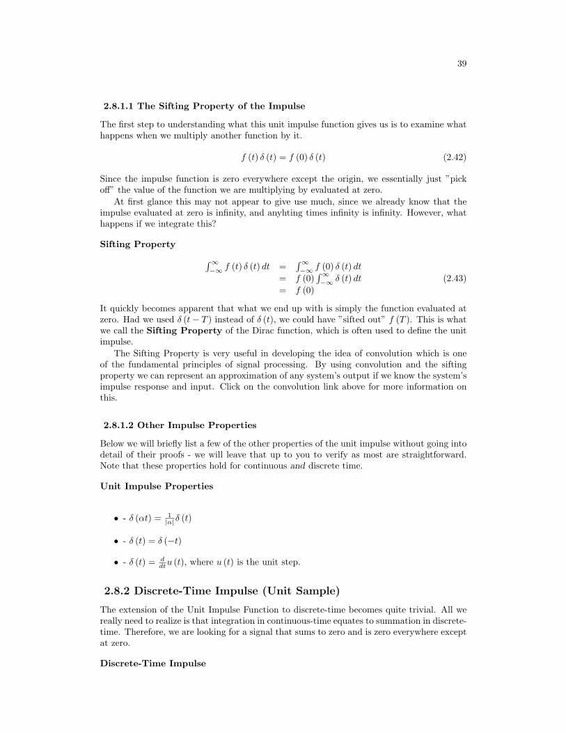
Figure 2.35: Since it is quite difficult to draw something that is infinitely tall, werepresent the Dirac with an arrow centered at the point it is applied. If we wish to scaleit, we may write the value it is scaled by next to the point of the arrow. This is a unitimpulse (no scaling).
39
2.8.1.1 The Sifting Property of the Impulse
The first step to understanding what this unit impulse function gives us is to examine whathappens when we multiply another function by it.
f (t) δ (t) = f (0) δ (t) (2.42)
Since the impulse function is zero everywhere except the origin, we essentially just ”pickoff” the value of the function we are multiplying by evaluated at zero.
At first glance this may not appear to give use much, since we already know that theimpulse evaluated at zero is infinity, and anyhting times infinity is infinity. However, whathappens if we integrate this?
Sifting Property ∫∞−∞ f (t) δ (t) dt =
∫∞−∞ f (0) δ (t) dt
= f (0)∫∞−∞ δ (t) dt
= f (0)(2.43)
It quickly becomes apparent that what we end up with is simply the function evaluated atzero. Had we used δ (t− T ) instead of δ (t), we could have ”sifted out” f (T ). This is whatwe call the Sifting Property of the Dirac function, which is often used to define the unitimpulse.
The Sifting Property is very useful in developing the idea of convolution which is oneof the fundamental principles of signal processing. By using convolution and the siftingproperty we can represent an approximation of any system’s output if we know the system’simpulse response and input. Click on the convolution link above for more information onthis.
2.8.1.2 Other Impulse Properties
Below we will briefly list a few of the other properties of the unit impulse without going intodetail of their proofs - we will leave that up to you to verify as most are straightforward.Note that these properties hold for continuous and discrete time.
Unit Impulse Properties
• - δ (αt) = 1|α|δ (t)
• - δ (t) = δ (−t)
• - δ (t) = ddtu (t), where u (t) is the unit step.
2.8.2 Discrete-Time Impulse (Unit Sample)
The extension of the Unit Impulse Function to discrete-time becomes quite trivial. All wereally need to realize is that integration in continuous-time equates to summation in discrete-time. Therefore, we are looking for a signal that sums to zero and is zero everywhere exceptat zero.
Discrete-Time Impulse
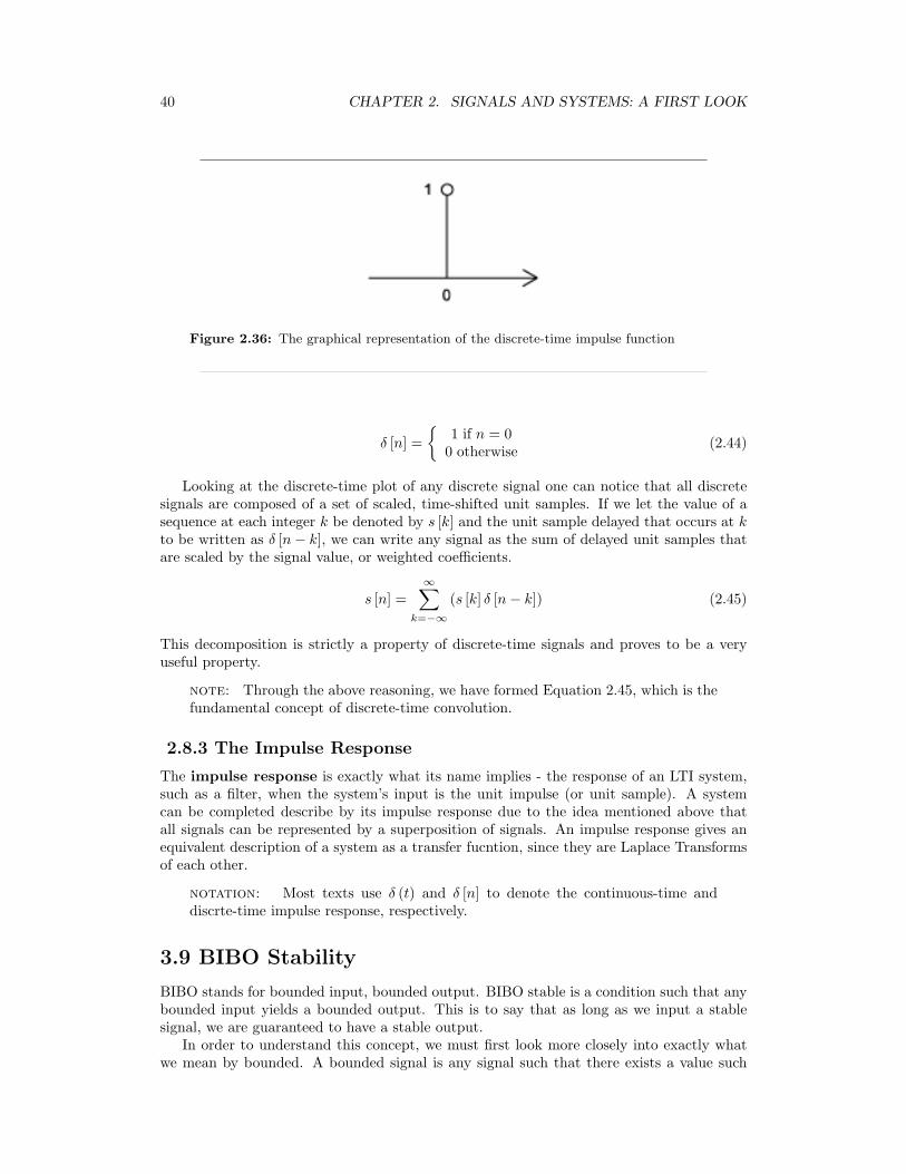
40 CHAPTER 2. SIGNALS AND SYSTEMS: A FIRST LOOK
Figure 2.36: The graphical representation of the discrete-time impulse function
δ [n] =
1 if n = 00 otherwise (2.44)
Looking at the discrete-time plot of any discrete signal one can notice that all discretesignals are composed of a set of scaled, time-shifted unit samples. If we let the value of asequence at each integer k be denoted by s [k] and the unit sample delayed that occurs at kto be written as δ [n− k], we can write any signal as the sum of delayed unit samples thatare scaled by the signal value, or weighted coefficients.
s [n] =∞∑
k=−∞
(s [k] δ [n− k]) (2.45)
This decomposition is strictly a property of discrete-time signals and proves to be a veryuseful property.
note: Through the above reasoning, we have formed Equation 2.45, which is thefundamental concept of discrete-time convolution.
2.8.3 The Impulse Response
The impulse response is exactly what its name implies - the response of an LTI system,such as a filter, when the system’s input is the unit impulse (or unit sample). A systemcan be completed describe by its impulse response due to the idea mentioned above thatall signals can be represented by a superposition of signals. An impulse response gives anequivalent description of a system as a transfer fucntion, since they are Laplace Transformsof each other.
notation: Most texts use δ (t) and δ [n] to denote the continuous-time anddiscrte-time impulse response, respectively.
3.9 BIBO Stability
BIBO stands for bounded input, bounded output. BIBO stable is a condition such that anybounded input yields a bounded output. This is to say that as long as we input a stablesignal, we are guaranteed to have a stable output.
In order to understand this concept, we must first look more closely into exactly whatwe mean by bounded. A bounded signal is any signal such that there exists a value such
41
Figure 2.37: A bounded signal is a signal for which there exists a constant A such that∀t : |f (t) | < A
that the absolute value of the signal is never greater than some value. Since this value isarbitrary, what we mean is that at no point can the signal tend to infinity.
Once we have identified what it means for a signal to be bounded, we must turn ourattention to the condition a system must posess in order to guarantee that if any boundedsignal is passed through the system, a bounded signal will arise on the output. It turns outthat a continuous-time LTI system with impulse response h (t) is BIBO stable if and onlyif
Continuous-Time Condition for BIBO Stability∫ ∞
−∞|h (t) |dt <∞ (2.46)
This is to say that the transfer function is absolutely integrable.To extend this concept to discrete-time, we make the standard transition from integration
to summation and get that the transfer function, h (n), must be absolutely summable. Thatis
Discrete-Time Condition for BIBO Stability
∞∑n=−∞
(|h (n) |) <∞ (2.47)
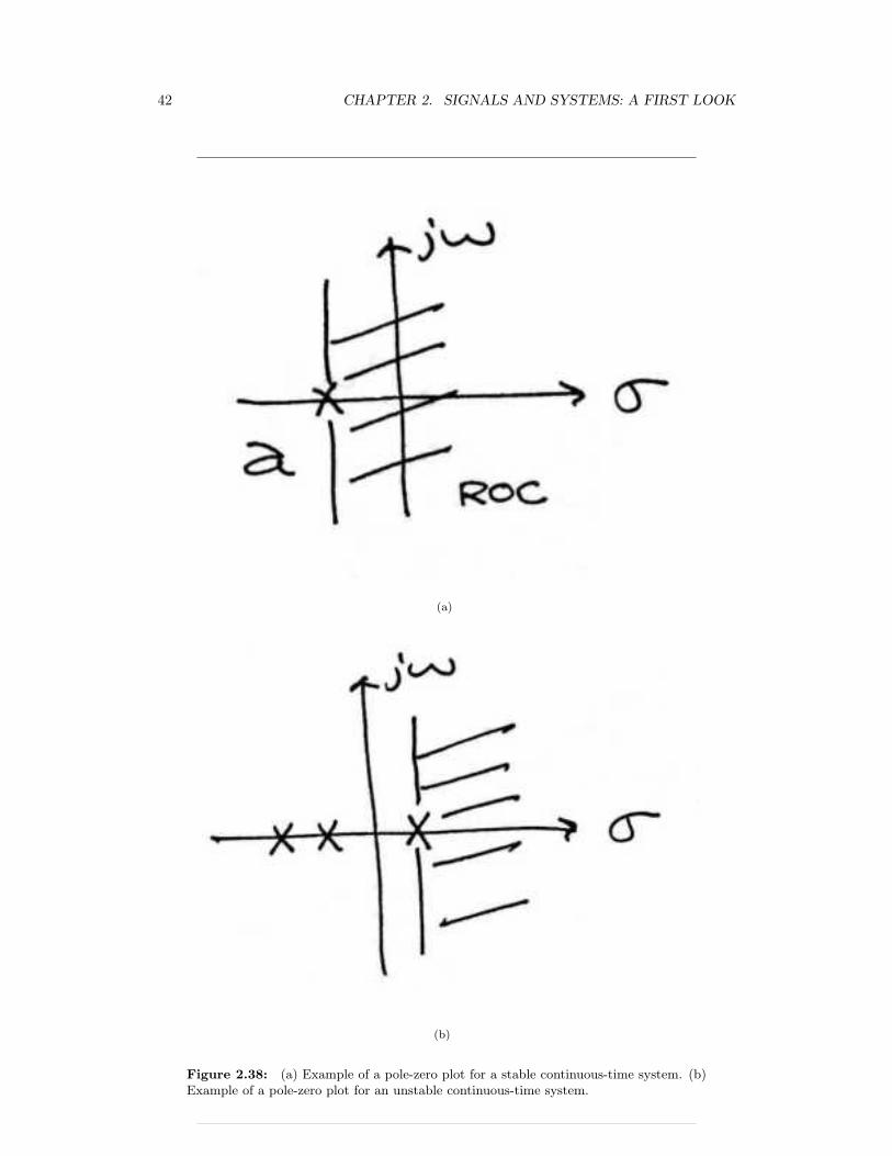
2.9.1 Stability and Laplace
Stability is very easy to infer from the pole-zero plot of a transfer function. The onlycondition necessary to demonstrate stability is to show that the jω-axis is in the region ofconvergence.
42 CHAPTER 2. SIGNALS AND SYSTEMS: A FIRST LOOK
(a)
(b)
Figure 2.38: (a) Example of a pole-zero plot for a stable continuous-time system. (b)Example of a pole-zero plot for an unstable continuous-time system.

43
2.9.2 Stability and the Z-Transform
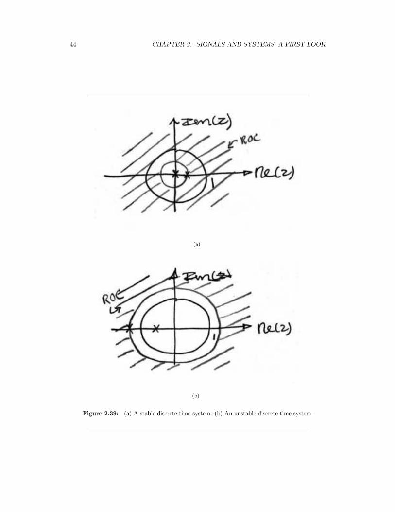
Stability for discrete-time signals in the z-domain is about as easy to demonstrate as itis for continuous-time signals in the Laplace domain. However, instead of the region ofconvergence needing to contain the jω-axis, the ROC must contain the unit circle.
44 CHAPTER 2. SIGNALS AND SYSTEMS: A FIRST LOOK
(a)
(b)
Figure 2.39: (a) A stable discrete-time system. (b) An unstable discrete-time system.
Chapter 3
Time-Domain Analysis of CTSystems
4.1 Systems in the Time-Domain
A discrete-time signal s (n) is delayed by n0 samples when we write s (n− n0), with n0 > 0.Choosing n0 to be negative advances the signal along the integers. As opposed to analogdelays (pg ??), discrete-time delays can only be integer valued. In the frequency domain,delaying a signal corresponds to a linear phase shift of the signal’s discrete-time Fouriertransform: s (n− n0) ↔ e−(j2πfn0)S
(ej2πf
).
Linear discrete-time systems have the superposition property.
Superposition
S (a1x1 (n) + a2x2 (n)) = a1S (x1 (n)) + a2S (x2 (n)) (3.1)
A discrete-time system is called shift-invariant (analogous to time-invariant analog sys-tems (pg ??)) if delaying the input delays the corresponding output.
Shift-Invariant
IfS (x (n)) = y (n) , ThenS (x (n− n0)) = y (n− n0) (3.2)
We use the term shift-invariant to emphasize that delays can only have integer values indiscrete-time, while in analog signals, delays can be arbitrarily valued.
We want to concentrate on systems that are both linear and shift-invariant. It willbe these that allow us the full power of frequency-domain analysis and implementations.Because we have no physical constraints in ”constructing” such systems, we need only amathematical specification. In analog systems, the differential equation specifies the input-output relationship in the time-domain. The corresponding discrete-time specification isthe difference equation .
The Difference Equation
y (n) = a1y (n− 1) + ...+ apy (n− p) + b0x (n) + b1x (n− 1) + ...+ bqx (n− q) (3.3)
Here, the output signal y (n) is related to its past values y (n− l), l = 1, ..., p, and to thecurrent and past values of the input signal x (n). The system’s characteristics are determinedby the choices for the number of coefficients p and q and the coefficients’ values a1, ..., apand b0, b1, ..., bq.
45
46 CHAPTER 3. TIME-DOMAIN ANALYSIS OF CT SYSTEMS
aside: There is an asymmetry in the coefficients: where is a0? This coefficientwould multiply the y (n) term in the difference equation (Equation 3.3). We haveessentially divided the equation by it, which does not change the input-outputrelationship. We have thus created the convention that a0 is always one.
As opposed to differential equations, which only provide an implicit description of asystem (we must somehow solve the differential equation), difference equations provide anexplicit way of computing the output for any input. We simply express the differenceequation by a program that calculates each output from the previous output values, andthe current and previous inputs.
4.2 Continuous-Time Convolution
3.2.1 Motivation
Convolution helps to determine the effect a system has on an input signal. It can be shownthat a linear, time-invariant system is completely characterized by its impulse response.At first glance, this may appear to be of little use, since impulse functions are not welldefnied in real applications. however, the sifting property of impulses (Section 2.8.1.1) tellsus that a signal can be decomposed into an infinite sum (integral) of scaled and shiftedimpulses. By knowing how a system affects a single impulse, and by understanding the waya signal is comprised of scaled and summed impulses, it seems reasonable that it should bepossible to scale and sum the impulse responses of a system in order to deteremine whatoutput signal will results from a particular input. This is precisely what convolution does -convolution determines the system’s output from knowledge of the input and the system’simpulse response.
In the rest of this module, we will examine exactly how convolution is defined from thereasoning above. This will result in the convolution integral (see the next section) and itsproperties. These concepts are very important in Electrical Engineering and will make anyengineer’s life a lot easier if the time is spent now to truly understand what is going on.
In order to fully understand convolution, you may find it useful to look at the discrete-time convolution as well. It will also be helpful to experiment with the applets1 availableon the internet. These resources will offer different approaches to this crucial concept.
3.2.2 Convolution Integral
As mentioned above, the convolution integral provides an easy mathematical way to expressthe output of an LTI system based on an arbitrary signal, x (t), and the system’s impulseresponse, h (t). The convolution integral is expressed as
y (t) =∫ ∞
−∞x (τ)h (t− τ) dτ (3.4)
Convolution is such an important tool that it is represented by the symbol *, and can bewritten as
y (t) = (x (t) , h (t)) (3.5)
By making a simple change of variables into the convolution integral, τ = t − τ , we caneasily show that convolution is commutative :
(x (t) , h (t)) = (h (t) , x (t)) (3.6)
1http://www.jhu.edu/∼signals
47
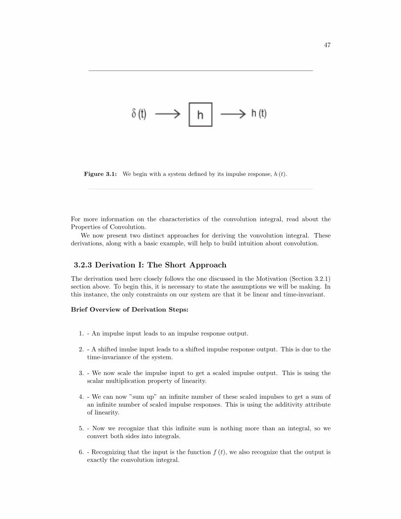
Figure 3.1: We begin with a system defined by its impulse response, h (t).
For more information on the characteristics of the convolution integral, read about theProperties of Convolution.
We now present two distinct approaches for deriving the vonvolution integral. Thesederivations, along with a basic example, will help to build intuition about convolution.
3.2.3 Derivation I: The Short Approach
The derivation used here closely follows the one discussed in the Motivation (Section 3.2.1)section above. To begin this, it is necessary to state the assumptions we will be making. Inthis instance, the only constraints on our system are that it be linear and time-invariant.
Brief Overview of Derivation Steps:
1. - An impulse input leads to an impulse response output.
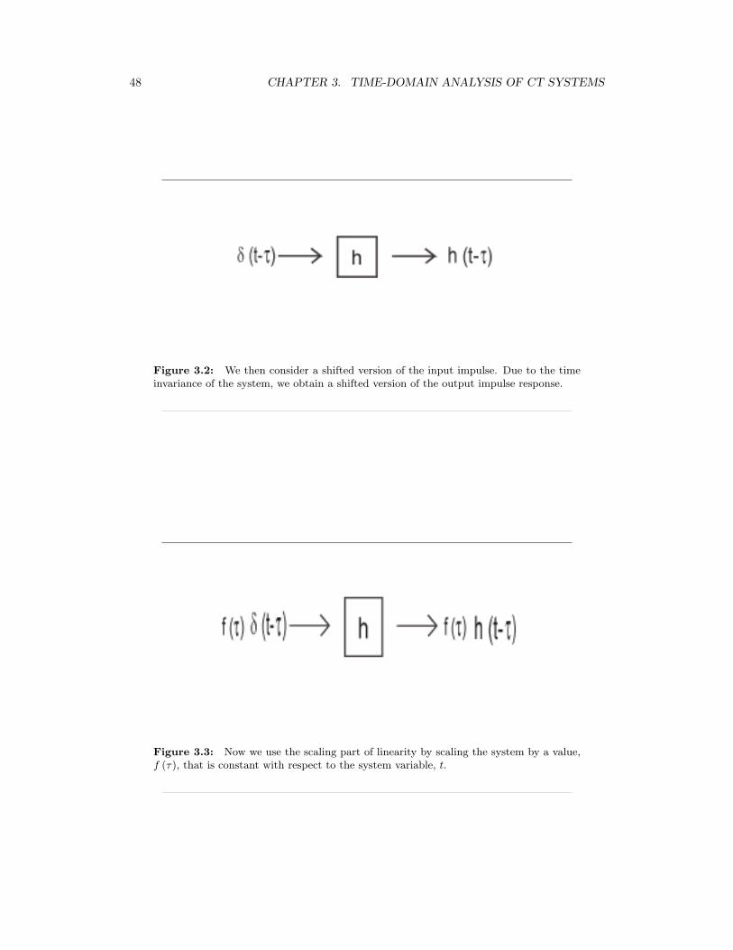
2. - A shifted imulse input leads to a shifted impulse response output. This is due to thetime-invariance of the system.
3. - We now scale the impulse input to get a scaled impulse output. This is using thescalar multiplication property of linearity.
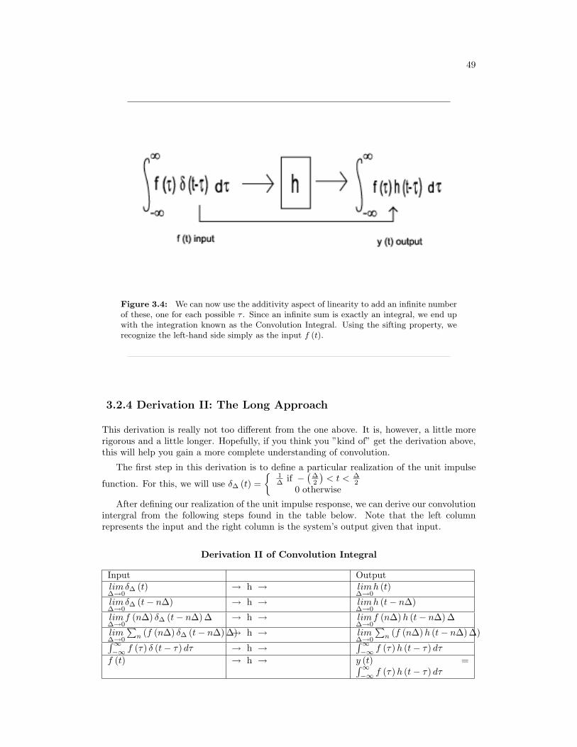
4. - We can now ”sum up” an infinite number of these scaled impulses to get a sum ofan infinite number of scaled impulse responses. This is using the additivity attributeof linearity.
5. - Now we recognize that this infinite sum is nothing more than an integral, so weconvert both sides into integrals.
6. - Recognizing that the input is the function f (t), we also recognize that the output isexactly the convolution integral.
48 CHAPTER 3. TIME-DOMAIN ANALYSIS OF CT SYSTEMS
Figure 3.2: We then consider a shifted version of the input impulse. Due to the timeinvariance of the system, we obtain a shifted version of the output impulse response.
Figure 3.3: Now we use the scaling part of linearity by scaling the system by a value,f (τ), that is constant with respect to the system variable, t.
49
Figure 3.4: We can now use the additivity aspect of linearity to add an infinite numberof these, one for each possible τ . Since an infinite sum is exactly an integral, we end upwith the integration known as the Convolution Integral. Using the sifting property, werecognize the left-hand side simply as the input f (t).
3.2.4 Derivation II: The Long Approach
This derivation is really not too different from the one above. It is, however, a little morerigorous and a little longer. Hopefully, if you think you ”kind of” get the derivation above,this will help you gain a more complete understanding of convolution.
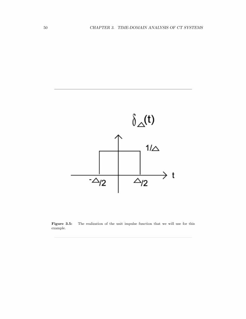
The first step in this derivation is to define a particular realization of the unit impulse
function. For this, we will use δ∆ (t) =
1∆ if −
(∆2
)< t < ∆
20 otherwise
After defining our realization of the unit impulse response, we can derive our convolutionintergral from the following steps found in the table below. Note that the left columnrepresents the input and the right column is the system’s output given that input.
Derivation II of Convolution Integral
Input Outputlim∆→0
δ∆ (t) → h → lim∆→0
h (t)
lim∆→0
δ∆ (t− n∆) → h → lim∆→0
h (t− n∆)
lim∆→0
f (n∆) δ∆ (t− n∆) ∆ → h → lim∆→0
f (n∆)h (t− n∆) ∆
lim∆→0
∑n (f (n∆) δ∆ (t− n∆) ∆)→ h → lim
∆→0
∑n (f (n∆)h (t− n∆) ∆)∫∞
−∞ f (τ) δ (t− τ) dτ → h →∫∞−∞ f (τ)h (t− τ) dτ
f (t) → h → y (t) =∫∞−∞ f (τ)h (t− τ) dτ
50 CHAPTER 3. TIME-DOMAIN ANALYSIS OF CT SYSTEMS
Figure 3.5: The realization of the unit impulse function that we will use for thisexample.
51
(a) (b)
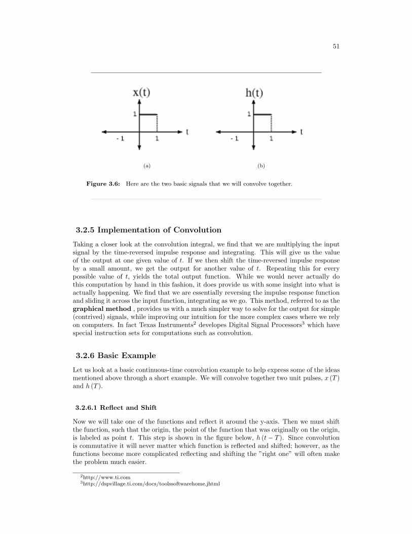
Figure 3.6: Here are the two basic signals that we will convolve together.
3.2.5 Implementation of Convolution
Taking a closer look at the convolution integral, we find that we are multiplying the inputsignal by the time-reversed impulse response and integrating. This will give us the valueof the output at one given value of t. If we then shift the time-reversed impulse responseby a small amount, we get the output for another value of t. Repeating this for everypossible value of t, yields the total output function. While we would never actually dothis computation by hand in this fashion, it does provide us with some insight into what isactually happening. We find that we are essentially reversing the impulse response functionand sliding it across the input function, integrating as we go. This method, referred to as thegraphical method , provides us with a much simpler way to solve for the output for simple(contrived) signals, while improving our intuition for the more complex cases where we relyon computers. In fact Texas Instruments2 developes Digital Signal Processors3 which havespecial instruction sets for computations such as convolution.
3.2.6 Basic Example
Let us look at a basic continuous-time convolution example to help express some of the ideasmentioned above through a short example. We will convolve together two unit pulses, x (T )and h (T ).
3.2.6.1 Reflect and Shift
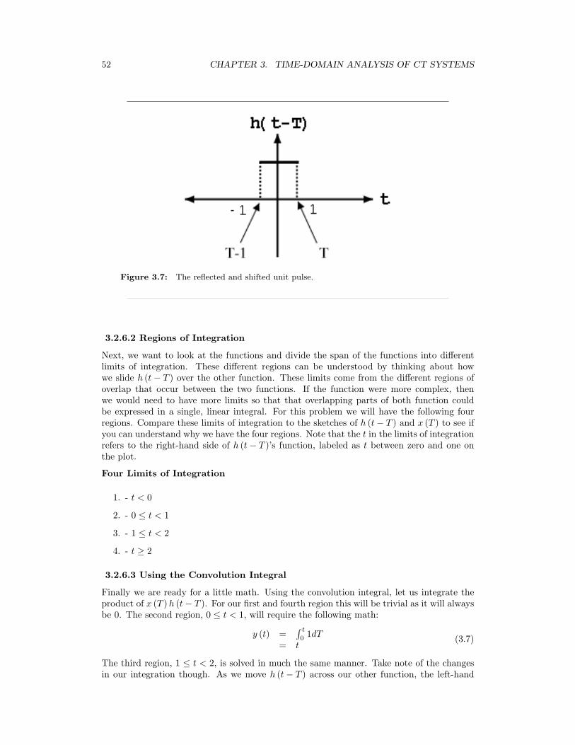
Now we will take one of the functions and reflect it around the y-axis. Then we must shiftthe function, such that the origin, the point of the function that was originally on the origin,is labeled as point t. This step is shown in the figure below, h (t− T ). Since convolutionis commutative it will never matter which function is reflected and shifted; however, as thefunctions become more complicated reflecting and shifting the ”right one” will often makethe problem much easier.
2http://www.ti.com3http://dspvillage.ti.com/docs/toolssoftwarehome.jhtml
52 CHAPTER 3. TIME-DOMAIN ANALYSIS OF CT SYSTEMS
Figure 3.7: The reflected and shifted unit pulse.
3.2.6.2 Regions of Integration
Next, we want to look at the functions and divide the span of the functions into differentlimits of integration. These different regions can be understood by thinking about howwe slide h (t− T ) over the other function. These limits come from the different regions ofoverlap that occur between the two functions. If the function were more complex, thenwe would need to have more limits so that that overlapping parts of both function couldbe expressed in a single, linear integral. For this problem we will have the following fourregions. Compare these limits of integration to the sketches of h (t− T ) and x (T ) to see ifyou can understand why we have the four regions. Note that the t in the limits of integrationrefers to the right-hand side of h (t− T )’s function, labeled as t between zero and one onthe plot.
Four Limits of Integration
1. - t < 0
2. - 0 ≤ t < 1
3. - 1 ≤ t < 2
4. - t ≥ 2
3.2.6.3 Using the Convolution Integral
Finally we are ready for a little math. Using the convolution integral, let us integrate theproduct of x (T )h (t− T ). For our first and fourth region this will be trivial as it will alwaysbe 0. The second region, 0 ≤ t < 1, will require the following math:
y (t) =∫ t
01dT
= t(3.7)
The third region, 1 ≤ t < 2, is solved in much the same manner. Take note of the changesin our integration though. As we move h (t− T ) across our other function, the left-hand
53
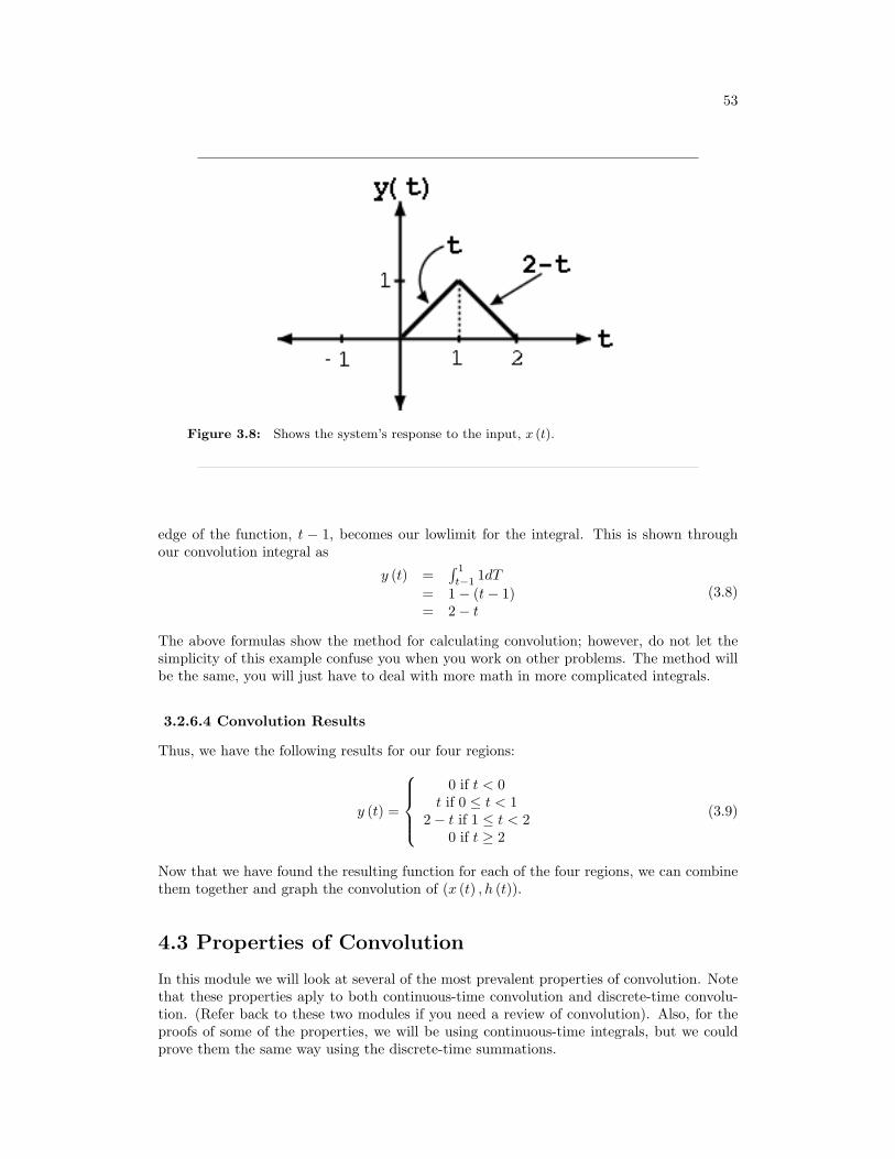
Figure 3.8: Shows the system’s response to the input, x (t).
edge of the function, t − 1, becomes our lowlimit for the integral. This is shown throughour convolution integral as
y (t) =∫ 1
t−11dT
= 1− (t− 1)= 2− t
(3.8)
The above formulas show the method for calculating convolution; however, do not let thesimplicity of this example confuse you when you work on other problems. The method willbe the same, you will just have to deal with more math in more complicated integrals.
3.2.6.4 Convolution Results
Thus, we have the following results for our four regions:
y (t) =
0 if t < 0
t if 0 ≤ t < 12− t if 1 ≤ t < 2
0 if t ≥ 2
(3.9)
Now that we have found the resulting function for each of the four regions, we can combinethem together and graph the convolution of (x (t) , h (t)).
4.3 Properties of Convolution
In this module we will look at several of the most prevalent properties of convolution. Notethat these properties aply to both continuous-time convolution and discrete-time convolu-tion. (Refer back to these two modules if you need a review of convolution). Also, for theproofs of some of the properties, we will be using continuous-time integrals, but we couldprove them the same way using the discrete-time summations.
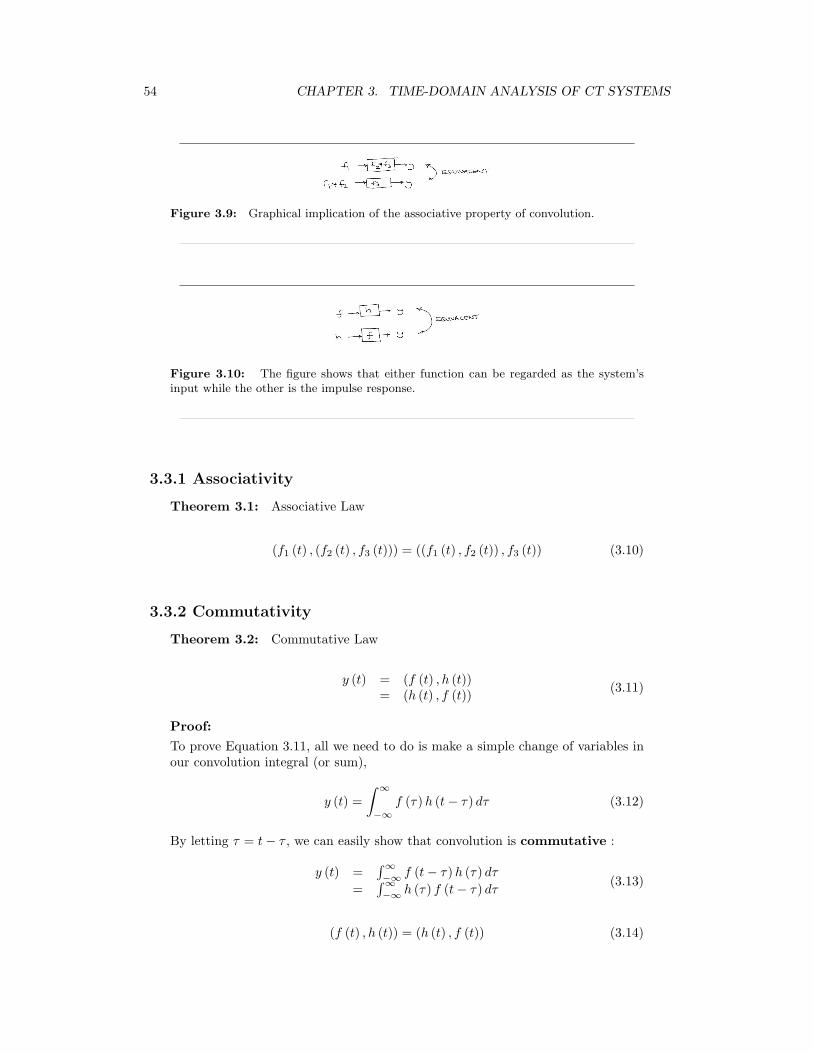
54 CHAPTER 3. TIME-DOMAIN ANALYSIS OF CT SYSTEMS
Figure 3.9: Graphical implication of the associative property of convolution.
Figure 3.10: The figure shows that either function can be regarded as the system’sinput while the other is the impulse response.
3.3.1 Associativity
Theorem 3.1: Associative Law
(f1 (t) , (f2 (t) , f3 (t))) = ((f1 (t) , f2 (t)) , f3 (t)) (3.10)
3.3.2 Commutativity
Theorem 3.2: Commutative Law
y (t) = (f (t) , h (t))= (h (t) , f (t)) (3.11)
Proof:
To prove Equation 3.11, all we need to do is make a simple change of variables inour convolution integral (or sum),
y (t) =∫ ∞
−∞f (τ)h (t− τ) dτ (3.12)
By letting τ = t− τ , we can easily show that convolution is commutative :
y (t) =∫∞−∞ f (t− τ)h (τ) dτ
=∫∞−∞ h (τ) f (t− τ) dτ
(3.13)
(f (t) , h (t)) = (h (t) , f (t)) (3.14)
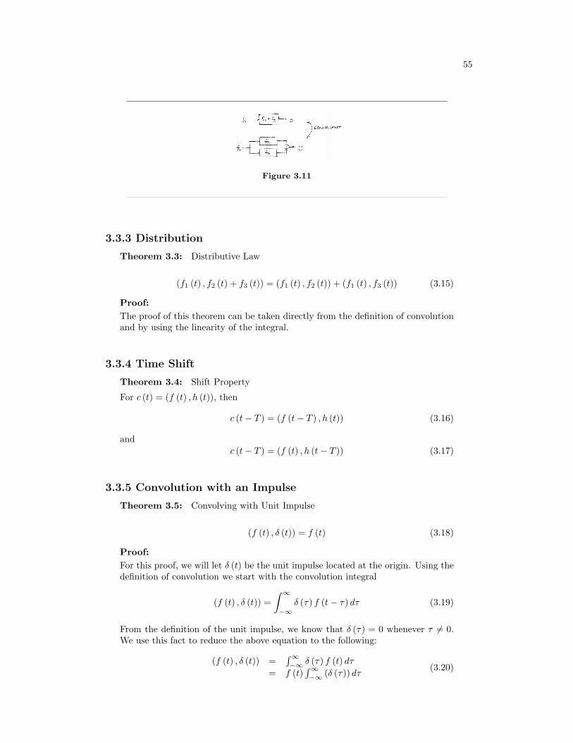
55
Figure 3.11
3.3.3 Distribution
Theorem 3.3: Distributive Law
(f1 (t) , f2 (t) + f3 (t)) = (f1 (t) , f2 (t)) + (f1 (t) , f3 (t)) (3.15)
Proof:The proof of this theorem can be taken directly from the definition of convolutionand by using the linearity of the integral.
3.3.4 Time Shift
Theorem 3.4: Shift Property
For c (t) = (f (t) , h (t)), then
c (t− T ) = (f (t− T ) , h (t)) (3.16)
andc (t− T ) = (f (t) , h (t− T )) (3.17)
3.3.5 Convolution with an Impulse
Theorem 3.5: Convolving with Unit Impulse
(f (t) , δ (t)) = f (t) (3.18)
Proof:For this proof, we will let δ (t) be the unit impulse located at the origin. Using thedefinition of convolution we start with the convolution integral
(f (t) , δ (t)) =∫ ∞
−∞δ (τ) f (t− τ) dτ (3.19)
From the definition of the unit impulse, we know that δ (τ) = 0 whenever τ 6= 0.We use this fact to reduce the above equation to the following:
(f (t) , δ (t)) =∫∞−∞ δ (τ) f (t) dτ
= f (t)∫∞−∞ (δ (τ)) dτ
(3.20)
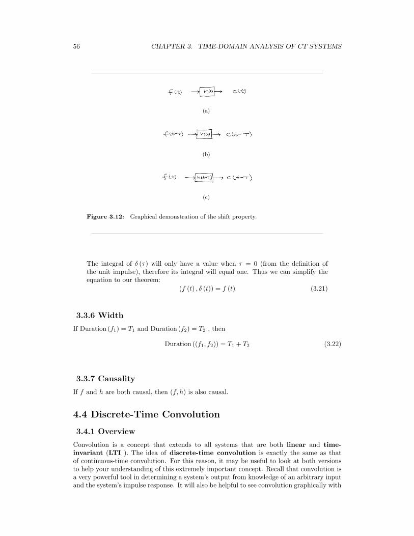
56 CHAPTER 3. TIME-DOMAIN ANALYSIS OF CT SYSTEMS
(a)
(b)
(c)
Figure 3.12: Graphical demonstration of the shift property.
The integral of δ (τ) will only have a value when τ = 0 (from the definition ofthe unit impulse), therefore its integral will equal one. Thus we can simplify theequation to our theorem:
(f (t) , δ (t)) = f (t) (3.21)
3.3.6 Width
If Duration (f1) = T1 and Duration (f2) = T2 , then
Duration ((f1, f2)) = T1 + T2 (3.22)
3.3.7 Causality
If f and h are both causal, then (f, h) is also causal.
4.4 Discrete-Time Convolution
3.4.1 Overview
Convolution is a concept that extends to all systems that are both linear and time-invariant (LTI ). The idea of discrete-time convolution is exactly the same as thatof continuous-time convolution. For this reason, it may be useful to look at both versionsto help your understanding of this extremely important concept. Recall that convolution isa very powerful tool in determining a system’s output from knowledge of an arbitrary inputand the system’s impulse response. It will also be helpful to see convolution graphically with
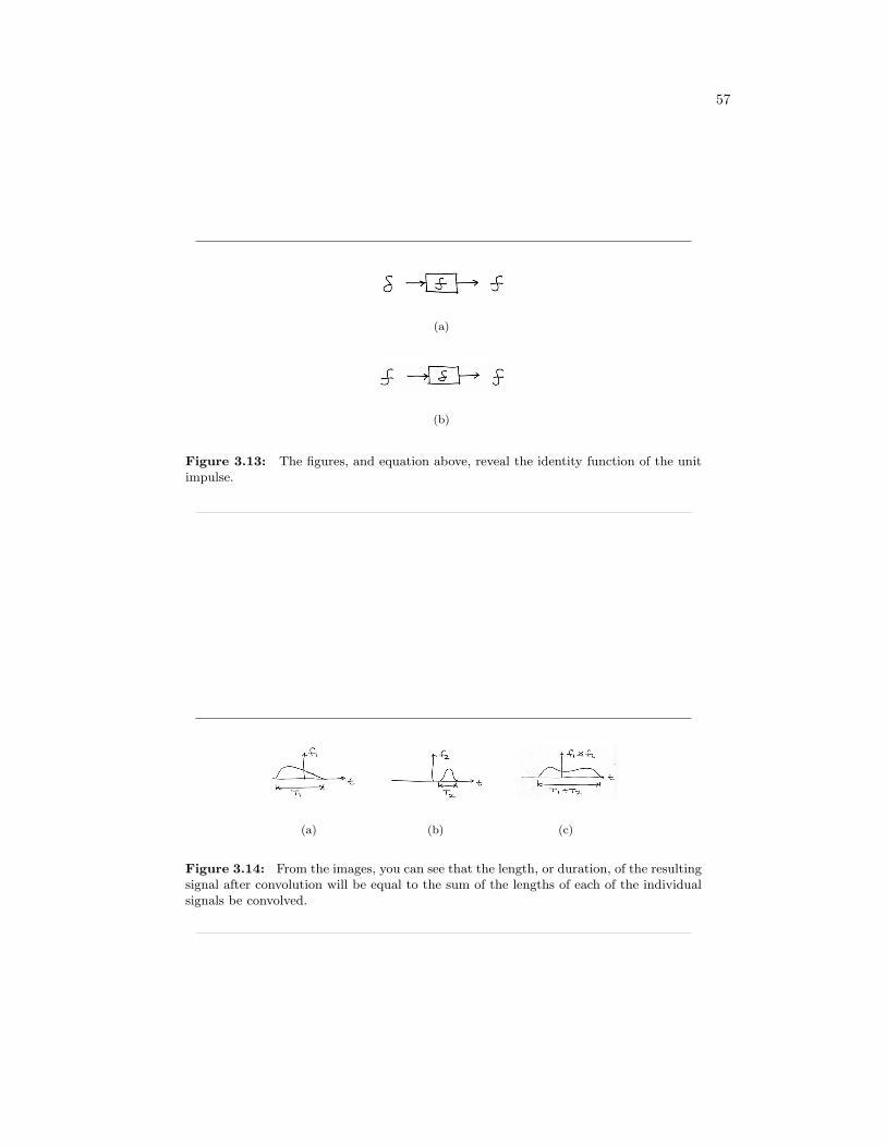
57
(a)
(b)
Figure 3.13: The figures, and equation above, reveal the identity function of the unitimpulse.
(a) (b) (c)
Figure 3.14: From the images, you can see that the length, or duration, of the resultingsignal after convolution will be equal to the sum of the lengths of each of the individualsignals be convolved.
58 CHAPTER 3. TIME-DOMAIN ANALYSIS OF CT SYSTEMS
your own eyes and to play around with it some, so experiment with the applets4 availableon the internet. These resources will offer different approaches to this crucial concept.
3.4.2 Convolution Sum
As mentioned above, the convolution sum provides a concise, mathematical way to expressthe output of an LTI system based on an arbitrary discrete-time input signal and the system’sresponse. The convolution sum is expressed as
y [n] =∞∑
k=−∞
(x [k]h [n− k]) (3.23)
As with continuous-time, convolution is represented by the symbol *, and can be written as
y [t] = x [t] ∗ h [t] (3.24)
By making a simple change of variables into the convolution sum, k = n− k, we can easilyshow that convolution is commutative :
x [t] ∗ h [t] = h [t] ∗ x [t] (3.25)
For more information on the characteristics of convolution, read about the Properties ofConvolution.
3.4.3 Derivation
We know that any discrete-time signal can be represented by a summation of scaled andshifted discrete-time impulses. Since we are assuming the system to be linear and time-invariant, it would seem to reason that an input signal comprised of the sum of scaled andshifted impulses would give rise to an output comprised of a sum of scaled and shiftedimpulse responses. This is exactly what occurs in convolution . Below we present a morerigorous and mathematical look at the derivation:
Letting H be a DT LTI system, we start with the folowing equation and work our waydown the the convoluation sum!
y [n] = H [x [n]]= H
[∑∞k=−∞ (x [k] δ [n− k])
]=
∑∞k=−∞ (H [x [k] δ [n− k]])
=∑∞
k=−∞ (x [k]H [δ [n− k]])=
∑∞k=−∞ (x [k]h [n− k])
(3.26)
Let us take a quick look at the steps taken in the above derivation. After our initial equation,we using the DT sifting property (Section 2.8.1.1) to rewrite the function, x [n], as a sumof the function times the unit impulse. Next, we can move around the H operator and thesummation because H [@] is a linear, DT system. Because of this linearity and the fact thatx [k] is a constannt, we can pull the previous mentioned constant out and simply multiplyit by H [@]. Finally, we use the fact that H [@] is time invariant in order to reach our finalstate - the convolution sum!
A quick graphical example may help in demonstrating why convolution works.
4http://www.jhu.edu/∼signals
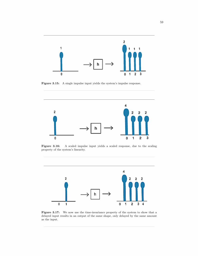
59
Figure 3.15: A single impulse input yields the system’s impulse response.
Figure 3.16: A scaled impulse input yields a scaled response, due to the scalingproperty of the system’s linearity.
Figure 3.17: We now use the time-invariance property of the system to show that adelayed input results in an output of the same shape, only delayed by the same amountas the input.
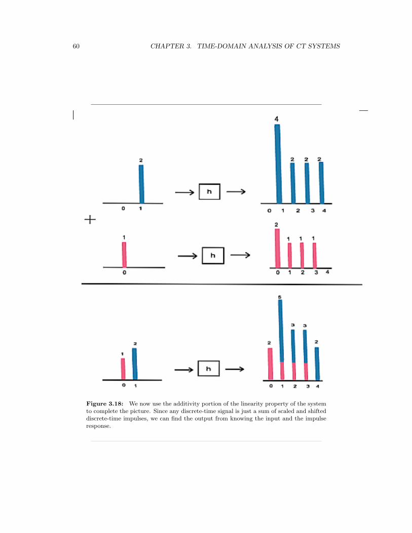
60 CHAPTER 3. TIME-DOMAIN ANALYSIS OF CT SYSTEMS
Figure 3.18: We now use the additivity portion of the linearity property of the systemto complete the picture. Since any discrete-time signal is just a sum of scaled and shifteddiscrete-time impulses, we can find the output from knowing the input and the impulseresponse.
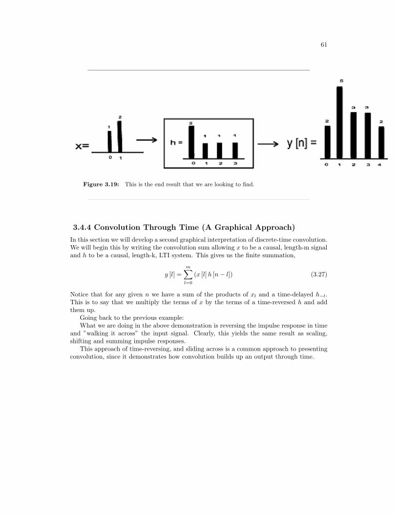
61
Figure 3.19: This is the end result that we are looking to find.
3.4.4 Convolution Through Time (A Graphical Approach)
In this section we will develop a second graphical interpretation of discrete-time convolution.We will begin this by writing the convolution sum allowing x to be a causal, length-m signaland h to be a causal, length-k, LTI system. This gives us the finite summation,
y [l] =m∑
l=0
(x [l]h [n− l]) (3.27)
Notice that for any given n we have a sum of the products of xl and a time-delayed h−l.This is to say that we multiply the terms of x by the terms of a time-reversed h and addthem up.
Going back to the previous example:What we are doing in the above demonstration is reversing the impulse response in time
and ”walking it across” the input signal. Clearly, this yields the same result as scaling,shifting and summing impulse responses.
This approach of time-reversing, and sliding across is a common approach to presentingconvolution, since it demonstrates how convolution builds up an output through time.
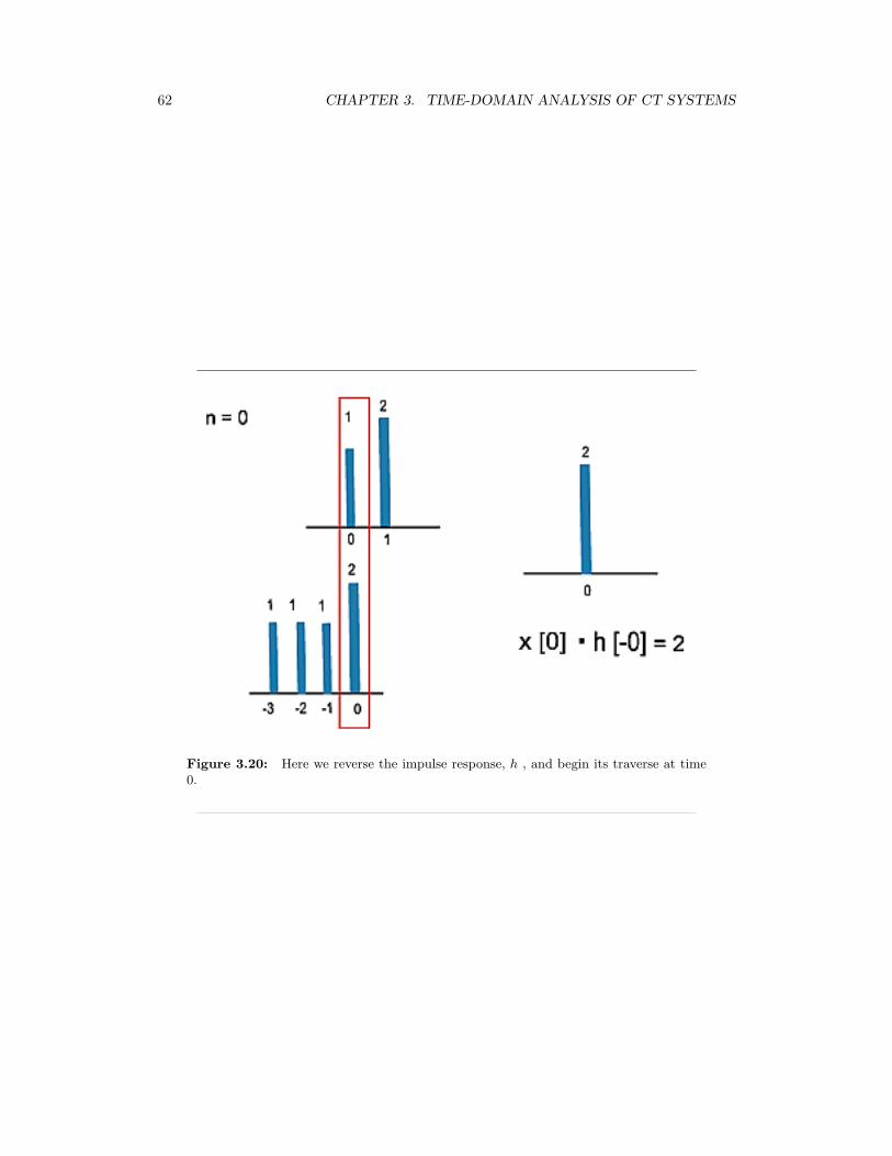
62 CHAPTER 3. TIME-DOMAIN ANALYSIS OF CT SYSTEMS
Figure 3.20: Here we reverse the impulse response, h , and begin its traverse at time0.
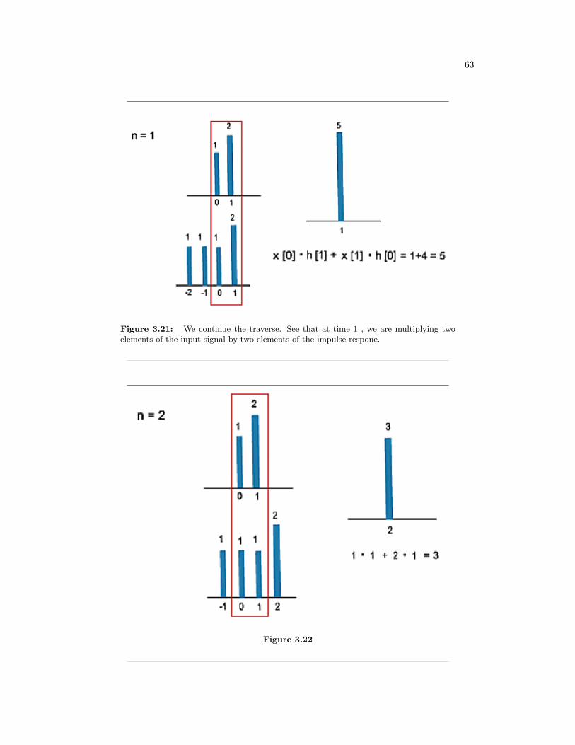
63
Figure 3.21: We continue the traverse. See that at time 1 , we are multiplying twoelements of the input signal by two elements of the impulse respone.
Figure 3.22
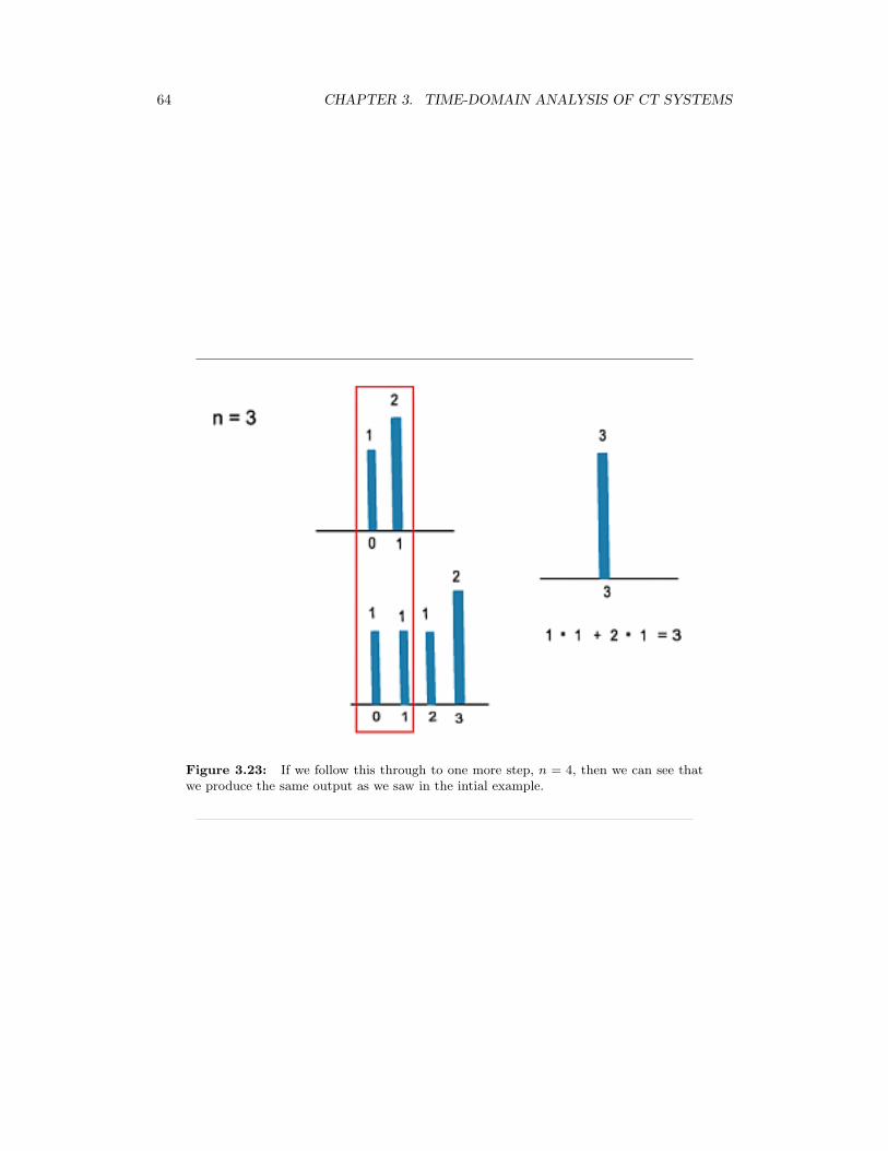
64 CHAPTER 3. TIME-DOMAIN ANALYSIS OF CT SYSTEMS
Figure 3.23: If we follow this through to one more step, n = 4, then we can see thatwe produce the same output as we saw in the intial example.
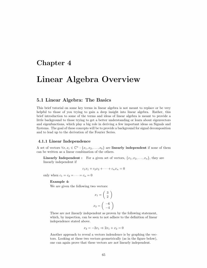
Chapter 4
Linear Algebra Overview
5.1 Linear Algebra: The Basics
This brief tutorial on some key terms in linear algebra is not meant to replace or be veryhelpful to those of you trying to gain a deep insight into linear algebra. Rather, thisbrief introduction to some of the terms and ideas of linear algebra is meant to provide alittle background to those trying to get a better understanding or learn about eigenvectorsand eigenfunctions, which play a big role in deriving a few important ideas on Signals andSystems. The goal of these concepts will be to provide a background for signal decompositionand to lead up to the derivation of the Fourier Series.
4.1.1 Linear Independence
A set of vectors ∀x, xi ∈ Cn : x1, x2, . . . , xk are linearly independent if none of themcan be written as a linear combination of the others.
Linearly Independent : For a given set of vectors, x1, x2, . . . , xn, they arelinearly independent if
c1x1 + c2x2 + · · ·+ cnxn = 0
only when c1 = c2 = · · · = cn = 0
Example 4:We are given the following two vectors:
x1 =(
32
)
x2 =(−6−4
)These are not linearly independent as proven by the following statement,which, by inspection, can be seen to not adhere to the definition of linearindependence stated above.
x2 = −2x1 ⇒ 2x1 + x2 = 0
Another approach to reveal a vectors indendence is by graphing the vec-tors. Looking at these two vectors geometrically (as in the figure below),one can again prove that these vectors are not linearly independent.
65
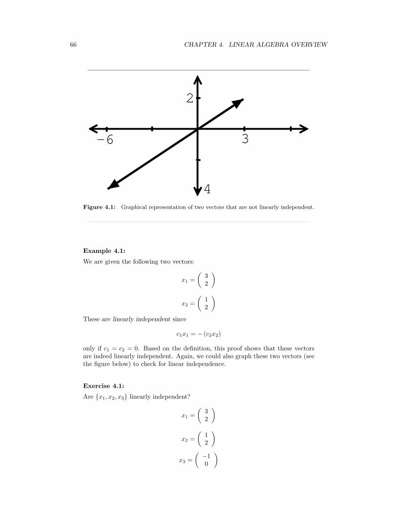
66 CHAPTER 4. LINEAR ALGEBRA OVERVIEW
3-6
2
4Figure 4.1: Graphical representation of two vectors that are not linearly independent.
Example 4.1:
We are given the following two vectors:
x1 =(
32
)
x2 =(
12
)These are linearly independent since
c1x1 = − (c2x2)
only if c1 = c2 = 0. Based on the definition, this proof shows that these vectorsare indeed linearly independent. Again, we could also graph these two vectors (seethe figure below) to check for linear independence.
Exercise 4.1:
Are x1, x2, x3 linearly independent?
x1 =(
32
)
x2 =(
12
)
x3 =(−10
)
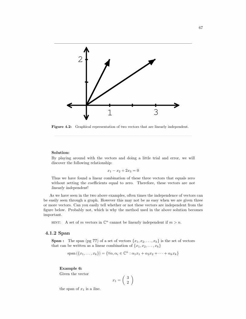
67
3
2
1
Figure 4.2: Graphical representation of two vectors that are linearly independent.
Solution:By playing around with the vectors and doing a little trial and error, we willdiscover the following relationship:
x1 − x2 + 2x3 = 0
Thus we have found a linear combination of these three vectors that equals zerowithout setting the coefficients equal to zero. Therefore, these vectors are notlinearly independent!
As we have seen in the two above examples, often times the independence of vectors canbe easily seen through a graph. However this may not be as easy when we are given threeor more vectors. Can you easily tell whether or not these vectors are independent from thefigure below. Probably not, which is why the method used in the above solution becomesimportant.
hint: A set of m vectors in Cn cannot be linearly independent if m > n.
4.1.2 Span
Span : The span (pg ??) of a set of vectors x1, x2, . . . , xk is the set of vectorsthat can be written as a linear combination of x1, x2, . . . , xk
span (x1, . . . , xk) = ∀α, αi ∈ Cn : α1x1 + α2x2 + · · ·+ αkxk
Example 6:Given the vector
x1 =(
32
)the span of x1 is a line.
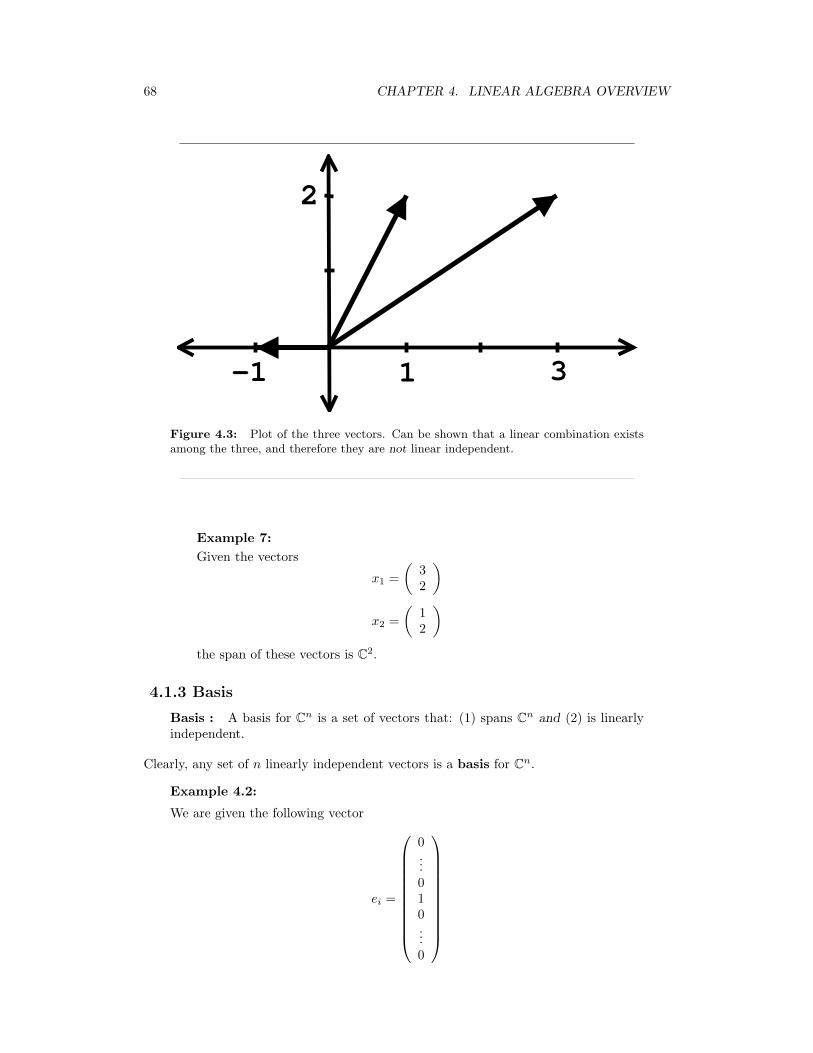
68 CHAPTER 4. LINEAR ALGEBRA OVERVIEW
3
2
1-1
Figure 4.3: Plot of the three vectors. Can be shown that a linear combination existsamong the three, and therefore they are not linear independent.
Example 7:Given the vectors
x1 =(
32
)x2 =
(12
)the span of these vectors is C2.
4.1.3 Basis
Basis : A basis for Cn is a set of vectors that: (1) spans Cn and (2) is linearlyindependent.
Clearly, any set of n linearly independent vectors is a basis for Cn.
Example 4.2:
We are given the following vector
ei =
0...010...0
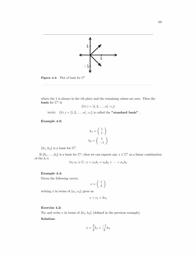
69
Figure 4.4: Plot of basis for C2
where the 1 is always in the ith place and the remaining values are zero. Then thebasis for Cn is
∀i, i = [1, 2, . . . , n] : ei
note: ∀i, i = [1, 2, . . . , n] : ei is called the ”standard basis” .
Example 4.3:
h1 =(
11
)h2 =
(1−1
)h1, h2 is a basis for C2.
If b1, . . . , b2 is a basis for Cn, then we can express any x ∈ Cn as a linear combinationof the bi’s:
∀α, αi ∈ C : x = α1b1 + α2b2 + · · ·+ αnbn
Example 4.4:
Given the following vector,
x =(
12
)writing x in terms of e1, e2 gives us
x = e1 + 2e2
Exercise 4.2:
Try and write x in terms of h1, h2 (defined in the previous example).
Solution:
x =32h1 +
−12h2
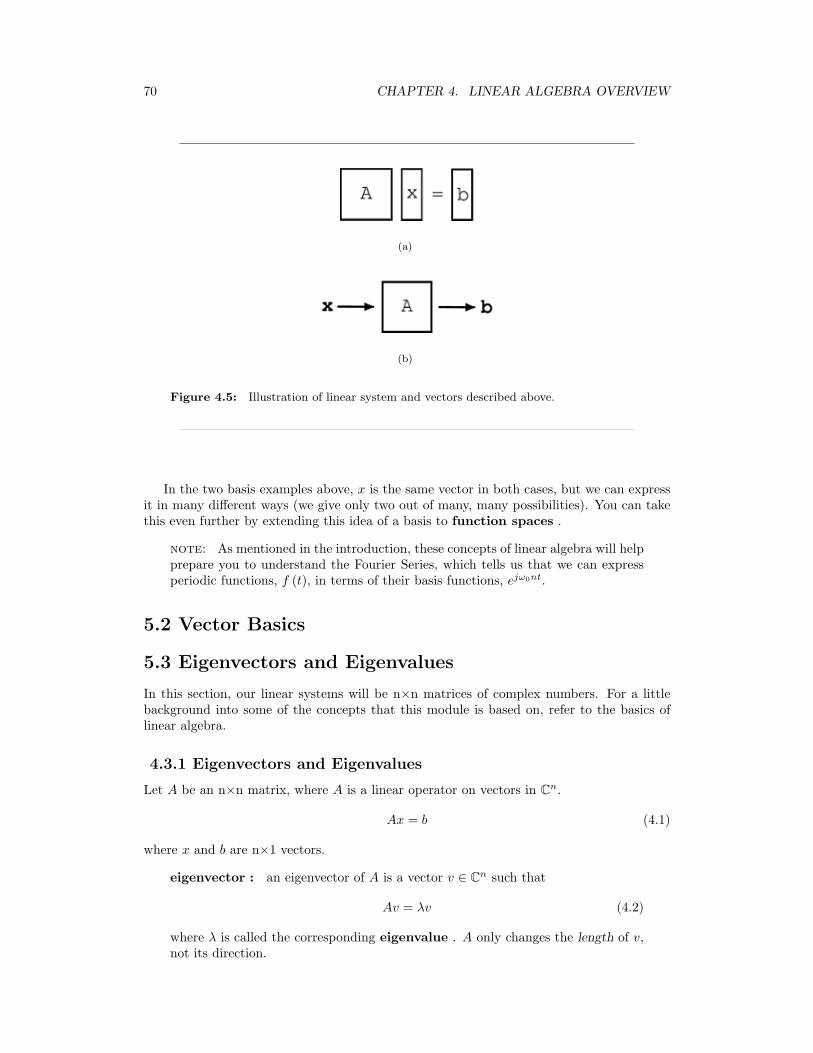
70 CHAPTER 4. LINEAR ALGEBRA OVERVIEW
(a)
(b)
Figure 4.5: Illustration of linear system and vectors described above.
In the two basis examples above, x is the same vector in both cases, but we can expressit in many different ways (we give only two out of many, many possibilities). You can takethis even further by extending this idea of a basis to function spaces .
note: As mentioned in the introduction, these concepts of linear algebra will helpprepare you to understand the Fourier Series, which tells us that we can expressperiodic functions, f (t), in terms of their basis functions, ejω0nt.
5.2 Vector Basics
5.3 Eigenvectors and Eigenvalues
In this section, our linear systems will be n×n matrices of complex numbers. For a littlebackground into some of the concepts that this module is based on, refer to the basics oflinear algebra.
4.3.1 Eigenvectors and Eigenvalues
Let A be an n×n matrix, where A is a linear operator on vectors in Cn.
Ax = b (4.1)
where x and b are n×1 vectors.
eigenvector : an eigenvector of A is a vector v ∈ Cn such that
Av = λv (4.2)
where λ is called the corresponding eigenvalue . A only changes the length of v,not its direction.
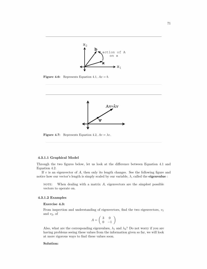
71
Figure 4.6: Represents Equation 4.1, Ax = b.
Figure 4.7: Represents Equation 4.2, Av = λv.
4.3.1.1 Graphical Model
Through the two figures below, let us look at the difference between Equation 4.1 andEquation 4.2.
If v is an eigenvector of A, then only its length changes. See the following figure andnotice how our vector’s length is simply scaled by our variable, λ, called the eigenvalue :
note: When dealing with a matrix A, eigenvectors are the simplest possiblevectors to operate on.
4.3.1.2 Examples
Exercise 4.3:
From inspection and understanding of eigenvectors, find the two eigenvectors, v1and v2, of
A =(
3 00 −1
)Also, what are the corresponding eigenvalues, λ1 and λ2? Do not worry if you arehaving problems seeing these values from the information given so far, we will lookat more rigorous ways to find these values soon.
Solution:
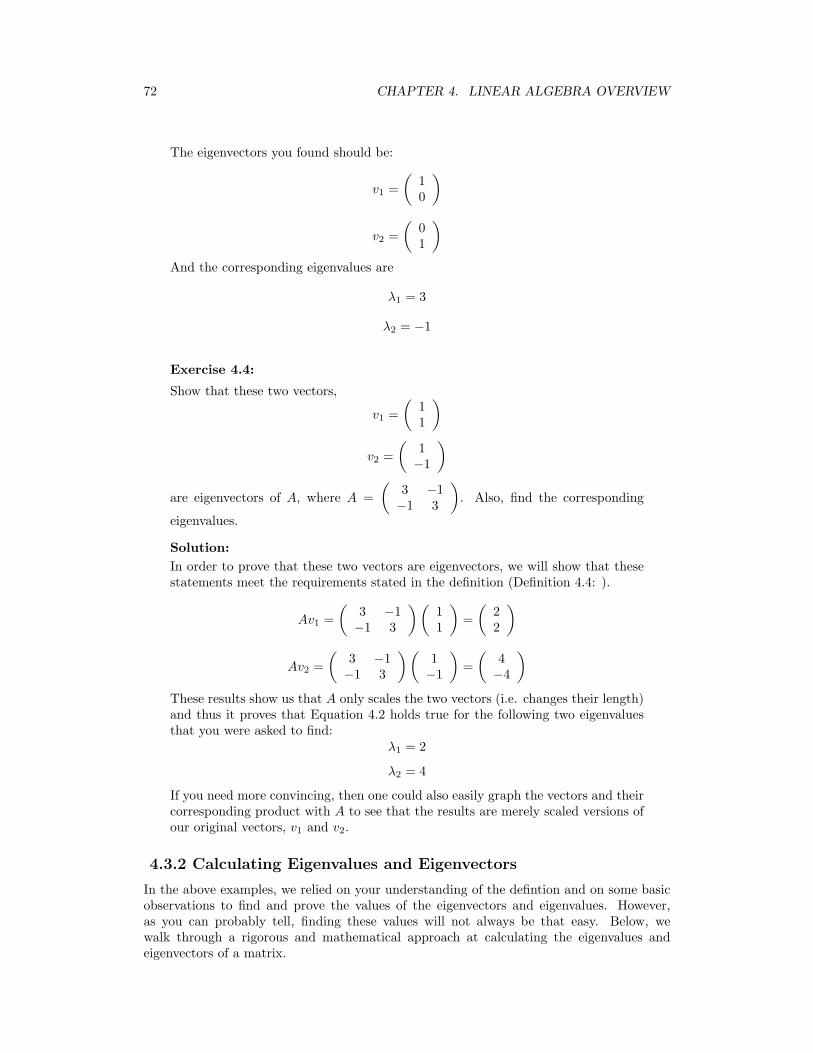
72 CHAPTER 4. LINEAR ALGEBRA OVERVIEW
The eigenvectors you found should be:
v1 =(
10
)
v2 =(
01
)And the corresponding eigenvalues are
λ1 = 3
λ2 = −1
Exercise 4.4:
Show that these two vectors,
v1 =(
11
)v2 =
(1−1
)are eigenvectors of A, where A =
(3 −1−1 3
). Also, find the corresponding
eigenvalues.
Solution:In order to prove that these two vectors are eigenvectors, we will show that thesestatements meet the requirements stated in the definition (Definition 4.4: ).
Av1 =(
3 −1−1 3
)(11
)=(
22
)
Av2 =(
3 −1−1 3
)(1−1
)=(
4−4
)These results show us that A only scales the two vectors (i.e. changes their length)and thus it proves that Equation 4.2 holds true for the following two eigenvaluesthat you were asked to find:
λ1 = 2
λ2 = 4
If you need more convincing, then one could also easily graph the vectors and theircorresponding product with A to see that the results are merely scaled versions ofour original vectors, v1 and v2.
4.3.2 Calculating Eigenvalues and Eigenvectors
In the above examples, we relied on your understanding of the defintion and on some basicobservations to find and prove the values of the eigenvectors and eigenvalues. However,as you can probably tell, finding these values will not always be that easy. Below, wewalk through a rigorous and mathematical approach at calculating the eigenvalues andeigenvectors of a matrix.
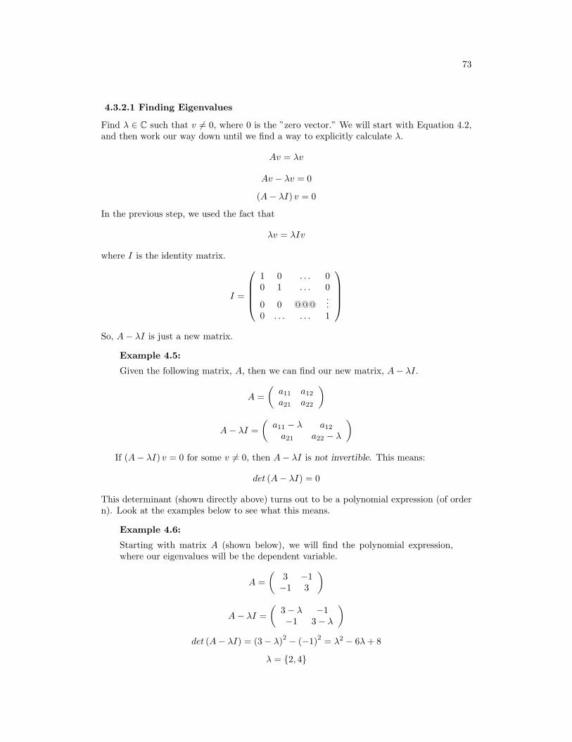
73
4.3.2.1 Finding Eigenvalues
Find λ ∈ C such that v 6= 0, where 0 is the ”zero vector.” We will start with Equation 4.2,and then work our way down until we find a way to explicitly calculate λ.
Av = λv
Av − λv = 0
(A− λI) v = 0
In the previous step, we used the fact that
λv = λIv
where I is the identity matrix.
I =
1 0 . . . 00 1 . . . 0
0 0 @@@...
0 . . . . . . 1
So, A− λI is just a new matrix.
Example 4.5:
Given the following matrix, A, then we can find our new matrix, A− λI.
A =(a11 a12
a21 a22
)
A− λI =(a11 − λ a12
a21 a22 − λ
)If (A− λI) v = 0 for some v 6= 0, then A− λI is not invertible. This means:
det (A− λI) = 0
This determinant (shown directly above) turns out to be a polynomial expression (of ordern). Look at the examples below to see what this means.
Example 4.6:
Starting with matrix A (shown below), we will find the polynomial expression,where our eigenvalues will be the dependent variable.
A =(
3 −1−1 3
)
A− λI =(
3− λ −1−1 3− λ
)det (A− λI) = (3− λ)2 − (−1)2 = λ2 − 6λ+ 8
λ = 2, 4
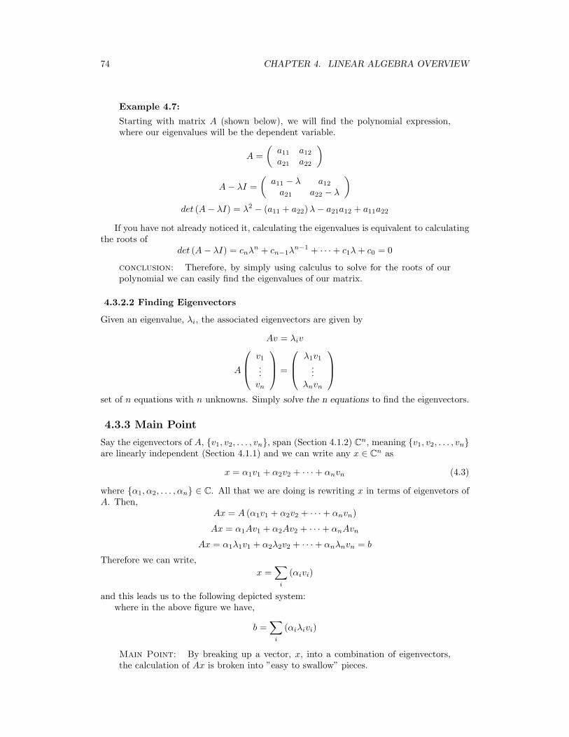
74 CHAPTER 4. LINEAR ALGEBRA OVERVIEW
Example 4.7:
Starting with matrix A (shown below), we will find the polynomial expression,where our eigenvalues will be the dependent variable.
A =(a11 a12
a21 a22
)
A− λI =(a11 − λ a12
a21 a22 − λ
)det (A− λI) = λ2 − (a11 + a22)λ− a21a12 + a11a22
If you have not already noticed it, calculating the eigenvalues is equivalent to calculatingthe roots of
det (A− λI) = cnλn + cn−1λ
n−1 + · · ·+ c1λ+ c0 = 0
conclusion: Therefore, by simply using calculus to solve for the roots of ourpolynomial we can easily find the eigenvalues of our matrix.
4.3.2.2 Finding Eigenvectors
Given an eigenvalue, λi, the associated eigenvectors are given by
Av = λiv
A
v1...vn
=
λ1v1...
λnvn
set of n equations with n unknowns. Simply solve the n equations to find the eigenvectors.
4.3.3 Main Point
Say the eigenvectors of A, v1, v2, . . . , vn, span (Section 4.1.2) Cn, meaning v1, v2, . . . , vnare linearly independent (Section 4.1.1) and we can write any x ∈ Cn as
x = α1v1 + α2v2 + · · ·+ αnvn (4.3)
where α1, α2, . . . , αn ∈ C. All that we are doing is rewriting x in terms of eigenvetors ofA. Then,
Ax = A (α1v1 + α2v2 + · · ·+ αnvn)
Ax = α1Av1 + α2Av2 + · · ·+ αnAvn
Ax = α1λ1v1 + α2λ2v2 + · · ·+ αnλnvn = b
Therefore we can write,x =
∑i
(αivi)
and this leads us to the following depicted system:where in the above figure we have,
b =∑
i
(αiλivi)
Main Point: By breaking up a vector, x, into a combination of eigenvectors,the calculation of Ax is broken into ”easy to swallow” pieces.
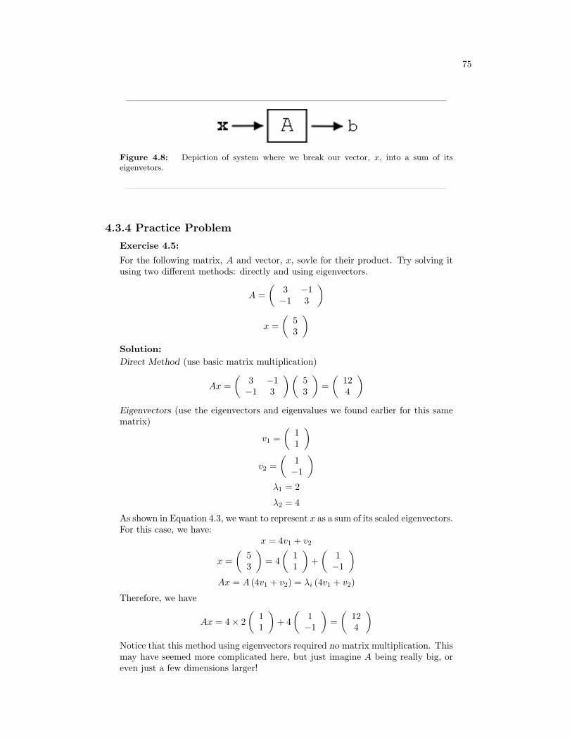
75
Figure 4.8: Depiction of system where we break our vector, x, into a sum of itseigenvetors.
4.3.4 Practice Problem
Exercise 4.5:
For the following matrix, A and vector, x, sovle for their product. Try solving itusing two different methods: directly and using eigenvectors.
A =(
3 −1−1 3
)
x =(
53
)Solution:Direct Method (use basic matrix multiplication)
Ax =(
3 −1−1 3
)(53
)=(
124
)Eigenvectors (use the eigenvectors and eigenvalues we found earlier for this samematrix)
v1 =(
11
)v2 =
(1−1
)λ1 = 2
λ2 = 4
As shown in Equation 4.3, we want to represent x as a sum of its scaled eigenvectors.For this case, we have:
x = 4v1 + v2
x =(
53
)= 4
(11
)+(
1−1
)Ax = A (4v1 + v2) = λi (4v1 + v2)
Therefore, we have
Ax = 4× 2(
11
)+ 4
(1−1
)=(
124
)Notice that this method using eigenvectors required no matrix multiplication. Thismay have seemed more complicated here, but just imagine A being really big, oreven just a few dimensions larger!
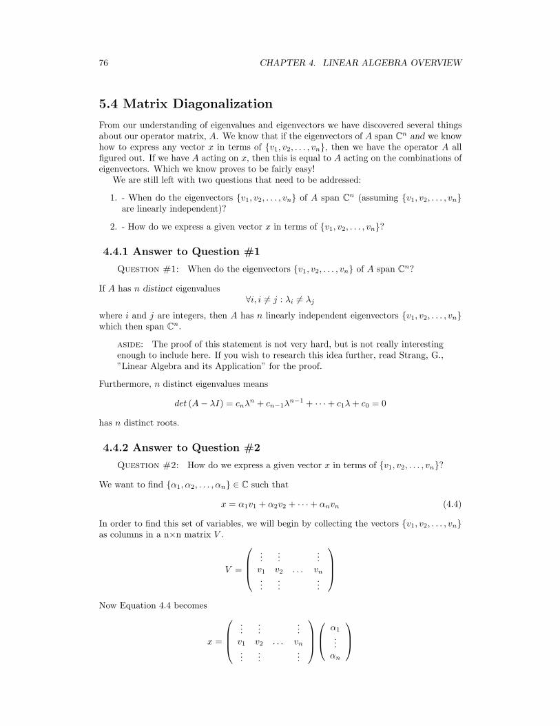
76 CHAPTER 4. LINEAR ALGEBRA OVERVIEW
5.4 Matrix Diagonalization
From our understanding of eigenvalues and eigenvectors we have discovered several thingsabout our operator matrix, A. We know that if the eigenvectors of A span Cn and we knowhow to express any vector x in terms of v1, v2, . . . , vn, then we have the operator A allfigured out. If we have A acting on x, then this is equal to A acting on the combinations ofeigenvectors. Which we know proves to be fairly easy!
We are still left with two questions that need to be addressed:
1. - When do the eigenvectors v1, v2, . . . , vn of A span Cn (assuming v1, v2, . . . , vnare linearly independent)?
2. - How do we express a given vector x in terms of v1, v2, . . . , vn?
4.4.1 Answer to Question #1
Question #1: When do the eigenvectors v1, v2, . . . , vn of A span Cn?
If A has n distinct eigenvalues∀i, i 6= j : λi 6= λj
where i and j are integers, then A has n linearly independent eigenvectors v1, v2, . . . , vnwhich then span Cn.
aside: The proof of this statement is not very hard, but is not really interestingenough to include here. If you wish to research this idea further, read Strang, G.,”Linear Algebra and its Application” for the proof.
Furthermore, n distinct eigenvalues means
det (A− λI) = cnλn + cn−1λ
n−1 + · · ·+ c1λ+ c0 = 0
has n distinct roots.
4.4.2 Answer to Question #2
Question #2: How do we express a given vector x in terms of v1, v2, . . . , vn?
We want to find α1, α2, . . . , αn ∈ C such that
x = α1v1 + α2v2 + · · ·+ αnvn (4.4)
In order to find this set of variables, we will begin by collecting the vectors v1, v2, . . . , vnas columns in a n×n matrix V .
V =
...
......
v1 v2 . . . vn
......
...
Now Equation 4.4 becomes
x =
...
......
v1 v2 . . . vn
......
...
α1
...αn
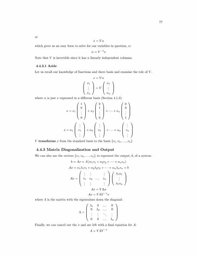
77
orx = V α
which gives us an easy form to solve for our variables in question, α:
α = V −1x
Note that V is invertible since it has n linearly independent columns.
4.4.2.1 Aside
Let us recall our knowledge of functions and there basis and examine the role of V .
x = V α x1
...xn
= V
α1
...αn
where α is just x expressed in a different basis (Section 4.1.3):
x = x1
10...0
+ x2
01...0
+ · · ·+ xn
00...1
x = α1
...v1...
+ α2
...v2...
+ · · ·+ αn
...vn
...
V transforms x from the standard basis to the basis v1, v2, . . . , vn
4.4.3 Matrix Diagonalization and Output
We can also use the vectors v1, v2, . . . , vn to represent the output, b, of a system:
b = Ax = A (α1v1 + α2v2 + · · ·+ αnvn)
Ax = α1λ1v1 + α2λ2v2 + · · ·+ αnλnvn = b
Ax =
...
......
v1 v2 . . . vn
......
...
λ1α1
...λ1αn
Ax = V Λα
Ax = V ΛV −1x
where Λ is the matrix with the eigenvalues down the diagonal:
Λ =
λ1 0 . . . 00 λ2 . . . 0...
.... . .
...0 0 . . . λn
Finally, we can cancel out the x and are left with a final equation for A:
A = V ΛV −1
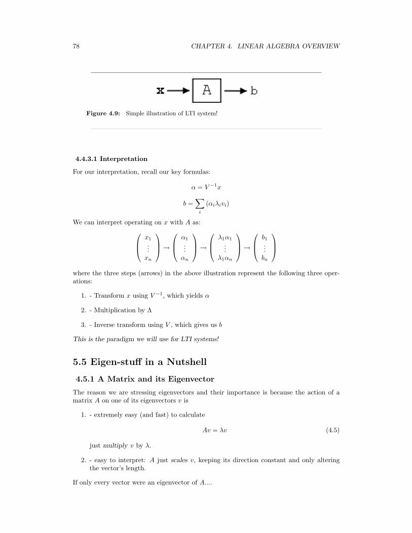
78 CHAPTER 4. LINEAR ALGEBRA OVERVIEW
Figure 4.9: Simple illustration of LTI system!
4.4.3.1 Interpretation
For our interpretation, recall our key formulas:
α = V −1x
b =∑
i
(αiλivi)
We can interpret operating on x with A as: x1
...xn
→
α1
...αn
→
λ1α1
...λ1αn
→
b1...bn
where the three steps (arrows) in the above illustration represent the following three oper-ations:
1. - Transform x using V −1, which yields α
2. - Multiplication by Λ
3. - Inverse transform using V , which gives us b
This is the paradigm we will use for LTI systems!
5.5 Eigen-stuff in a Nutshell
4.5.1 A Matrix and its Eigenvector
The reason we are stressing eigenvectors and their importance is because the action of amatrix A on one of its eigenvectors v is
1. - extremely easy (and fast) to calculate
Av = λv (4.5)
just multiply v by λ.
2. - easy to interpret: A just scales v, keeping its direction constant and only alteringthe vector’s length.
If only every vector were an eigenvector of A....
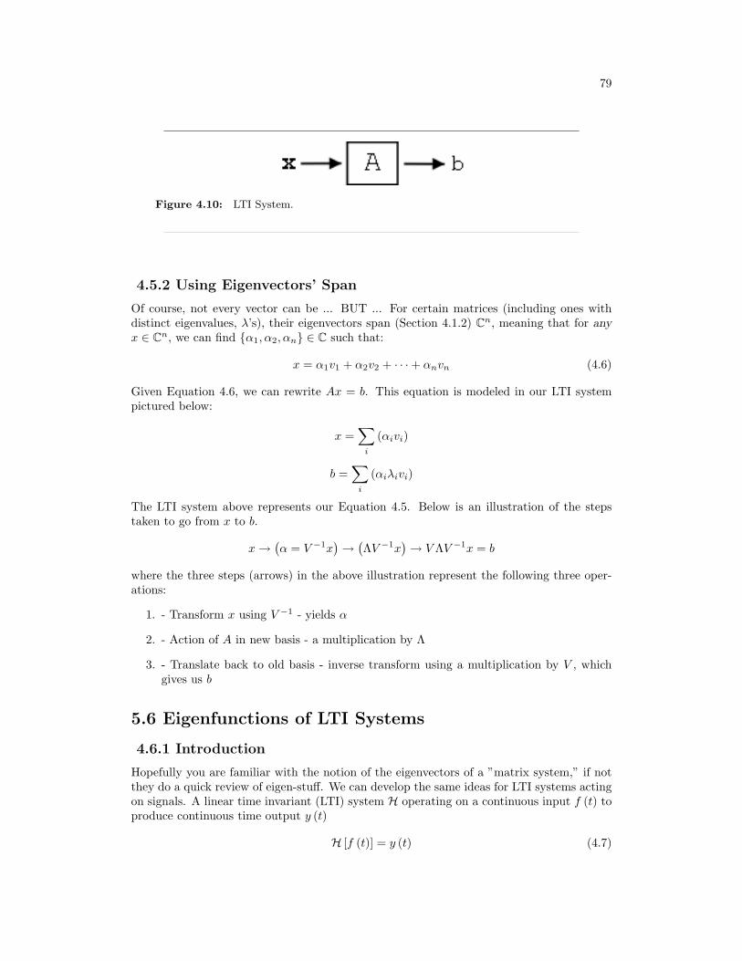
79
Figure 4.10: LTI System.
4.5.2 Using Eigenvectors’ Span
Of course, not every vector can be ... BUT ... For certain matrices (including ones withdistinct eigenvalues, λ’s), their eigenvectors span (Section 4.1.2) Cn, meaning that for anyx ∈ Cn, we can find α1, α2, αn ∈ C such that:
x = α1v1 + α2v2 + · · ·+ αnvn (4.6)
Given Equation 4.6, we can rewrite Ax = b. This equation is modeled in our LTI systempictured below:
x =∑
i
(αivi)
b =∑
i
(αiλivi)
The LTI system above represents our Equation 4.5. Below is an illustration of the stepstaken to go from x to b.
x→(α = V −1x
)→(ΛV −1x
)→ V ΛV −1x = b
where the three steps (arrows) in the above illustration represent the following three oper-ations:
1. - Transform x using V −1 - yields α
2. - Action of A in new basis - a multiplication by Λ
3. - Translate back to old basis - inverse transform using a multiplication by V , whichgives us b
5.6 Eigenfunctions of LTI Systems
4.6.1 Introduction
Hopefully you are familiar with the notion of the eigenvectors of a ”matrix system,” if notthey do a quick review of eigen-stuff. We can develop the same ideas for LTI systems actingon signals. A linear time invariant (LTI) system H operating on a continuous input f (t) toproduce continuous time output y (t)
H [f (t)] = y (t) (4.7)
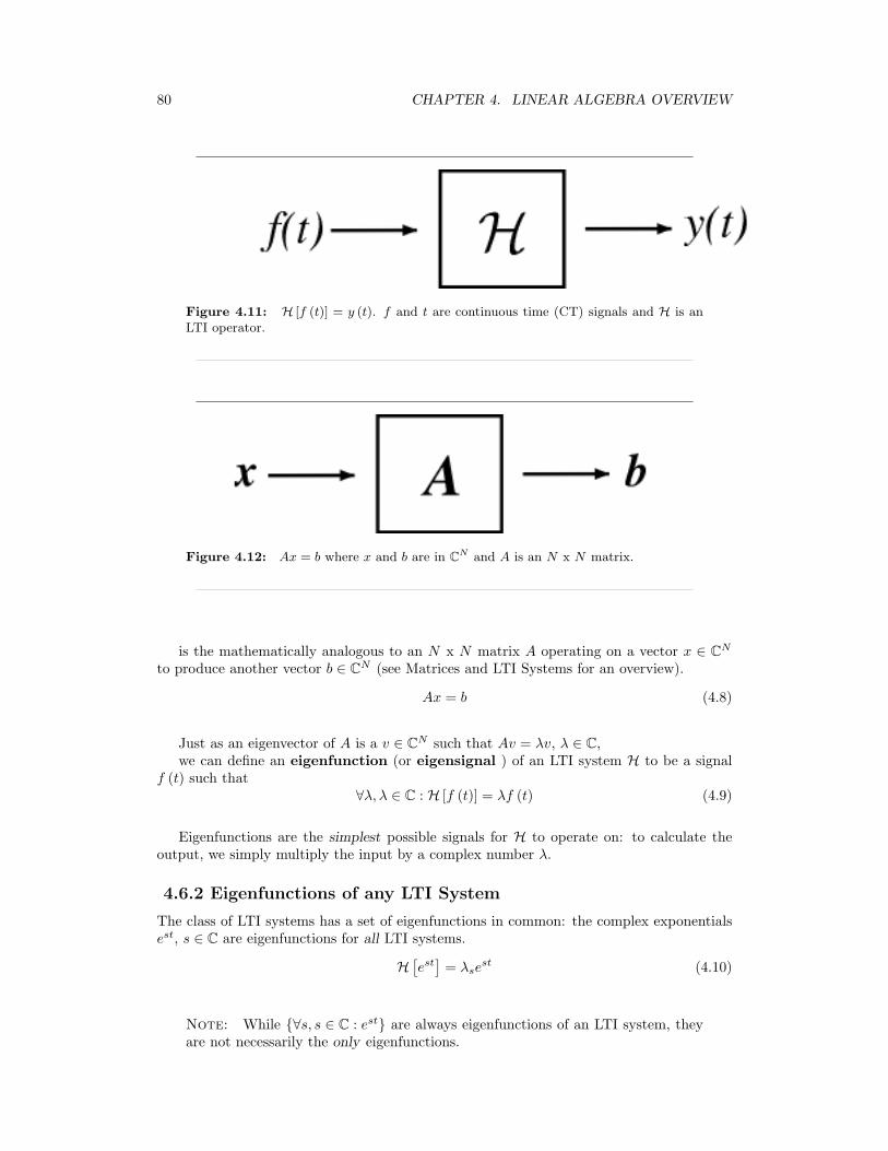
80 CHAPTER 4. LINEAR ALGEBRA OVERVIEW
Figure 4.11: H [f (t)] = y (t). f and t are continuous time (CT) signals and H is anLTI operator.
Figure 4.12: Ax = b where x and b are in CN and A is an N x N matrix.
is the mathematically analogous to an N x N matrix A operating on a vector x ∈ CN
to produce another vector b ∈ CN (see Matrices and LTI Systems for an overview).
Ax = b (4.8)
Just as an eigenvector of A is a v ∈ CN such that Av = λv, λ ∈ C,we can define an eigenfunction (or eigensignal ) of an LTI system H to be a signal
f (t) such that∀λ, λ ∈ C : H [f (t)] = λf (t) (4.9)
Eigenfunctions are the simplest possible signals for H to operate on: to calculate theoutput, we simply multiply the input by a complex number λ.
4.6.2 Eigenfunctions of any LTI System
The class of LTI systems has a set of eigenfunctions in common: the complex exponentialsest, s ∈ C are eigenfunctions for all LTI systems.
H[est]
= λsest (4.10)
Note: While ∀s, s ∈ C : est are always eigenfunctions of an LTI system, theyare not necessarily the only eigenfunctions.
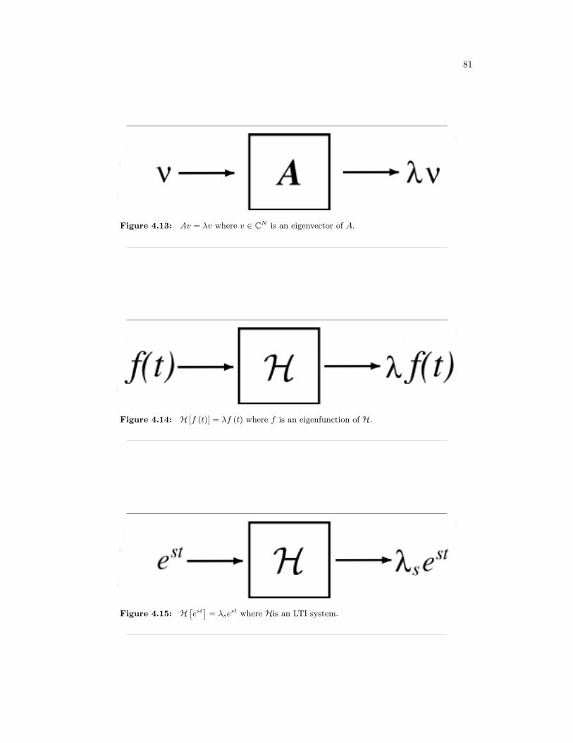
81
Figure 4.13: Av = λv where v ∈ CN is an eigenvector of A.
Figure 4.14: H [f (t)] = λf (t) where f is an eigenfunction of H.
Figure 4.15: H[est
]= λse
st where His an LTI system.
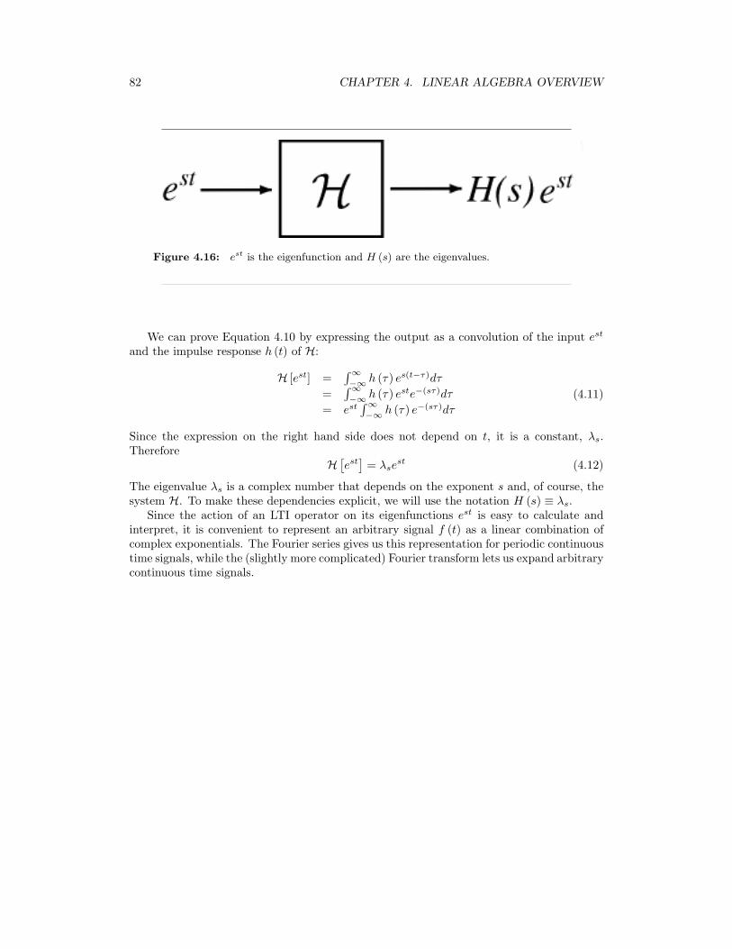
82 CHAPTER 4. LINEAR ALGEBRA OVERVIEW
Figure 4.16: est is the eigenfunction and H (s) are the eigenvalues.
We can prove Equation 4.10 by expressing the output as a convolution of the input est
and the impulse response h (t) of H:
H [est] =∫∞−∞ h (τ) es(t−τ)dτ
=∫∞−∞ h (τ) este−(sτ)dτ
= est∫∞−∞ h (τ) e−(sτ)dτ
(4.11)
Since the expression on the right hand side does not depend on t, it is a constant, λs.Therefore
H[est]
= λsest (4.12)
The eigenvalue λs is a complex number that depends on the exponent s and, of course, thesystem H. To make these dependencies explicit, we will use the notation H (s) ≡ λs.
Since the action of an LTI operator on its eigenfunctions est is easy to calculate andinterpret, it is convenient to represent an arbitrary signal f (t) as a linear combination ofcomplex exponentials. The Fourier series gives us this representation for periodic continuoustime signals, while the (slightly more complicated) Fourier transform lets us expand arbitrarycontinuous time signals.
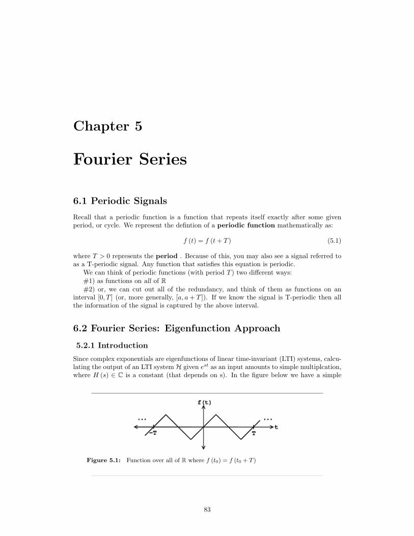
Chapter 5
Fourier Series
6.1 Periodic Signals
Recall that a periodic function is a function that repeats itself exactly after some givenperiod, or cycle. We represent the defintion of a periodic function mathematically as:
f (t) = f (t+ T ) (5.1)
where T > 0 represents the period . Because of this, you may also see a signal referred toas a T-periodic signal. Any function that satisfies this equation is periodic.
We can think of periodic functions (with period T ) two different ways:#1) as functions on all of R#2) or, we can cut out all of the redundancy, and think of them as functions on an
interval [0, T ] (or, more generally, [a, a+ T ]). If we know the signal is T-periodic then allthe information of the signal is captured by the above interval.
6.2 Fourier Series: Eigenfunction Approach
5.2.1 Introduction
Since complex exponentials are eigenfunctions of linear time-invariant (LTI) systems, calcu-lating the output of an LTI system H given est as an input amounts to simple multiplcation,where H (s) ∈ C is a constant (that depends on s). In the figure below we have a simple
Figure 5.1: Function over all of R where f (t0) = f (t0 + T )
83
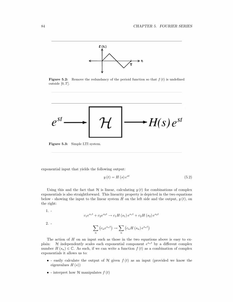
84 CHAPTER 5. FOURIER SERIES
Figure 5.2: Remove the redundancy of the perioid function so that f (t) is undefinedoutside [0, T ].
Figure 5.3: Simple LTI system.
exponential input that yields the following output:
y (t) = H (s) est (5.2)
Using this and the fact that H is linear, calculating y (t) for combinations of complexexponentials is also straightforward. This linearity property is depicted in the two equationsbelow - showing the input to the linear system H on the left side and the output, y (t), onthe right:
1. -c1e
s1t + c2es2t → c1H (s1) es1t + c2H (s2) es2t
2. - ∑n
(cne
snt)→∑
n
(cnH (sn) esnt
)The action of H on an input such as those in the two equations above is easy to ex-
plain: H independently scales each exponential component esnt by a different complexnumber H (sn) ∈ C. As such, if we can write a function f (t) as a combination of complexexponentials it allows us to:
• - easily calculate the output of H given f (t) as an input (provided we know theeigenvalues H (s))
• - interpret how H manipulates f (t)
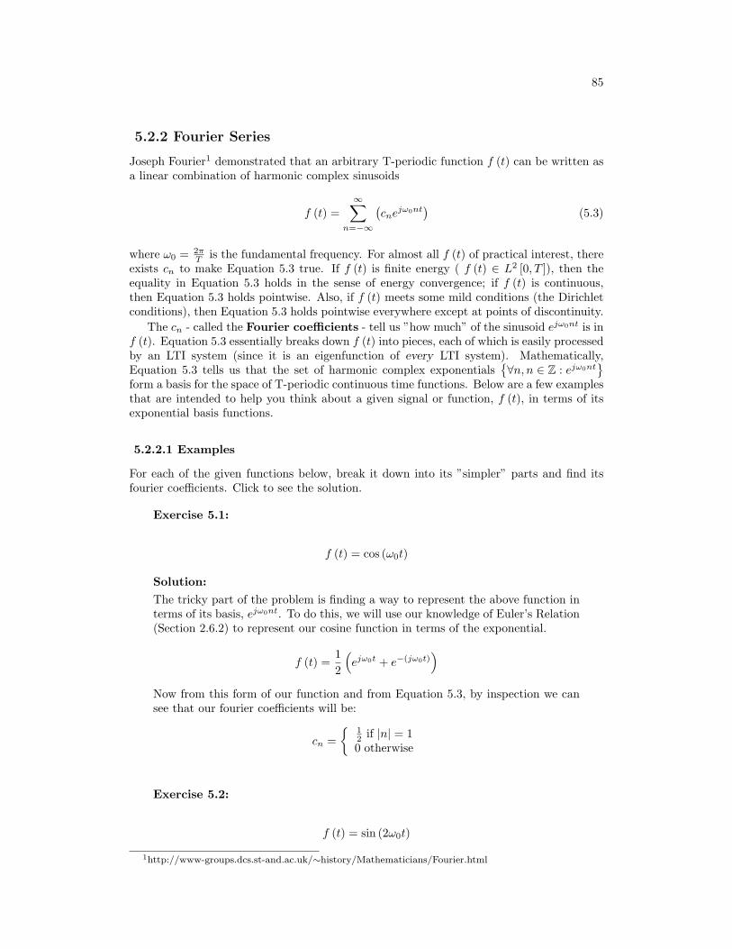
85
5.2.2 Fourier Series
Joseph Fourier1 demonstrated that an arbitrary T-periodic function f (t) can be written asa linear combination of harmonic complex sinusoids
f (t) =∞∑
n=−∞
(cne
jω0nt)
(5.3)
where ω0 = 2πT is the fundamental frequency. For almost all f (t) of practical interest, there
exists cn to make Equation 5.3 true. If f (t) is finite energy ( f (t) ∈ L2 [0, T ]), then theequality in Equation 5.3 holds in the sense of energy convergence; if f (t) is continuous,then Equation 5.3 holds pointwise. Also, if f (t) meets some mild conditions (the Dirichletconditions), then Equation 5.3 holds pointwise everywhere except at points of discontinuity.
The cn - called the Fourier coefficients - tell us ”how much” of the sinusoid ejω0nt is inf (t). Equation 5.3 essentially breaks down f (t) into pieces, each of which is easily processedby an LTI system (since it is an eigenfunction of every LTI system). Mathematically,Equation 5.3 tells us that the set of harmonic complex exponentials
∀n, n ∈ Z : ejω0nt
form a basis for the space of T-periodic continuous time functions. Below are a few examplesthat are intended to help you think about a given signal or function, f (t), in terms of itsexponential basis functions.
5.2.2.1 Examples
For each of the given functions below, break it down into its ”simpler” parts and find itsfourier coefficients. Click to see the solution.
Exercise 5.1:
f (t) = cos (ω0t)
Solution:The tricky part of the problem is finding a way to represent the above function interms of its basis, ejω0nt. To do this, we will use our knowledge of Euler’s Relation(Section 2.6.2) to represent our cosine function in terms of the exponential.
f (t) =12
(ejω0t + e−(jω0t)
)Now from this form of our function and from Equation 5.3, by inspection we cansee that our fourier coefficients will be:
cn =
12 if |n| = 10 otherwise
Exercise 5.2:
f (t) = sin (2ω0t)
1http://www-groups.dcs.st-and.ac.uk/∼history/Mathematicians/Fourier.html
86 CHAPTER 5. FOURIER SERIES
Solution:As done in the previous example, we will again use Euler’s Relation (Section 2.6.2)to represent our sine function in terms of exponential functions.
f (t) =12j
(ejω0t − e−(jω0t)
)And so our fourier coefficients are
cn =
−j2 if n = −1j2 if n = 1
0 otherwise
Exercise 5.3:
f (t) = 3 + 4cos (ω0t) + 2cos (2ω0t)
Solution:Once again we will use the same technique as was used in the previous two prob-lems. The break down of our function yields
f (t) = 3 + 4(
12
)(ejω0t + e−(jω0t)
)+ 2
(12
)(ej2ω0t + e−(j2ω0t)
)And from this we can find our fourier coefficients to be:
cn =
3 if n = 02 if |n| = 11 if |n| = 20 otherwise
5.2.3 Fourier Coefficients
In general f (t), the Fourier coefficients can be calculated from Equation 5.3 by solvingfor cn, which requires a little algebraic manipulation (for the complete derivation see theFourier coefficients derivation). The end results will yield the following general equation forthe fourier coefficients:
cn =1T
∫ T
0
f (t) e−(jω0nt)dt (5.4)
The sequence of complex numbers ∀n, n ∈ Z : cn is just an alternate representation of thefunction f (t). Knowing the Fourier coefficients cn is the same as knowing f (t) explicitlyand vice versa. Given a periodic function, we can transform it into it Fourier seriesrepresentation using Equation 5.4. Likewise, we can inverse transform a given sequenceof complex numbers, cn, using Equation 5.3 to reconstruct the function f (t).
Along with being a natural representation for signals being manipulated by LTI systems,the Fourier series provides a description of periodic signals that is convenient in many ways.By looking at the Fourier series of a signal f (t), we can infer mathematical properties of f (t)such as smoothness, existence of certain symmetries, as well as the physically meaningfulfrequency content.
87
5.2.3.1 Example: Using Fourier Coefficient Equation
Here we will look at a rather simple example that almost requires the use of Equation 5.4to solve for the fourier coefficients. Once you understand the formula, the solution becomesa straightforward calculus problem. Find the fourier coefficients for the following equation:
Exercise 5.4:
f (t) =
1 if |t| ≤ T0 otherwise
Solution:We will begin by plugging our above function, f (t), into Equation 5.4. Our intervalof integration will now change to match the interval specified by the function.
cn =1T
∫ T1
−T1
(1) e−(jω0nt)dt
Notice that we must consider two cases: n = 0 and n 6= 0. For n = 0 we can tellby inspection that we will get
∀n, n = 0 : cn =2T1
T
For n 6= 0, we will need to take a few more steps to solve. We can begin by lookingat the basic integral of the exponential we have. Remembering our calculus, weare ready to integrate:
cn =1T
(1
jω0n
)e−(jω0nt)|T1
t=−T1
Let us now evaluate the exponential functions for the given limits and expand ourequation to:
cn =1T
(1
− (jω0n)
)(e−(jω0nT1) − ejω0nT1
)Now if we multiple the right side of our equation by 2j
2j and distribute our negativesign into the parenthesis, we can utilize Euler’s Relation (Section 2.6.2) to greatlysimplify our expression into:
cn =1T
(2jjω0n
)sin (ω0nT1)
Now, recall earlier that we defined ω0 = 2πT . We can solve this equation for T and
substitute in.
cn =2jω0
jω0n2πsin (ω0nT1)
And finally, if we make a few simple cancellations we will arrive at our final answerfor the Fourier coefficients of f (t):
∀n, n 6= 0 : cn =sin (ω0nT1)
nπ
88 CHAPTER 5. FOURIER SERIES
5.2.4 Summary: Fourier Series Equations
Our first equation (Equation 5.3) is the synthesis equation, which builds our function,f (t), by combining sinusoids.
Synthesis
f (t) =∞∑
n=−∞
(cne
jω0nt)
(5.5)
And our second equation (Equation 5.4), termed the analysis equation, reveals how muchof each sinusoid is in f (t).
Analysis
cn =1T
∫ T
0
f (t) e−(jω0nt)dt (5.6)
where we have stated that ω0 = 2πT .
note: Understand that our interval of integration does not have to be [0, T ] inour Analysis Equation. We could use any interval [a, a+ T ] of length T .
6.3 Derivation of Fourier Coefficients Equation
5.3.1 Introduction
You should already be familiar with the existence of the general Fourier Series equation(Section 5.2.2), which is written as:
f (t) =∞∑
n=−∞
(cne
jω0nt)
(5.7)
What we are interested in here is how to determine the Fourier coefficients, cn, given afunction f (t). Below we will walk through the steps of deriving the general equation for theFourier coefficients of a given function.
5.3.2 Derivation
To solve Equation 5.7 for cn, we have to do a little algebraic manipulation. First of all wewill multiply both sides of Equation 5.7 by e−(jω0kt), where k ∈ Z.
f (t) e−(jω0kt) =∞∑
n=−∞
(cne
jω0nte−(jω0kt))
(5.8)
Now integrate both sides over a given period, T :∫ T
0
f (t) e−(jω0kt)dt =∫ T
0
∞∑n=−∞
(cne
jω0nte−(jω0kt))dt (5.9)
On the right-hand side we can switch the summation and integral along with pulling outthe constant out of the integral.∫ T
0
f (t) e−(jω0kt)dt =∞∑
n=−∞
(cn
∫ T
0
ejω0(n−k)tdt
)(5.10)
89
Now that we have made this seemingly more complicated, let us focus on just the integral,∫ T
0ejω0(n−k)tdt, on the right-hand side of the above equation. For this intergral we will need
to consider two cases: n = k and n 6= k. For n = k we will have:
∀n, n = k :∫ T
0
ejω0(n−k)tdt = T (5.11)
For n 6= k, we will have:
∀n, n 6= k :∫ T
0
ejω0(n−k)tdt =∫ T
0
cos (jω0 (n− k) t) dt+ j
∫ T
0
sin (jω0 (n− k) t) dt (5.12)
But cos (jω0 (n− k) t) has an integer number of periods, n− k, between 0 and T . Imaginea graph of the cosine; because it has an integer number of periods, there are equal areasabove and below the x-axis of the graph. This statemnt holds true for sin (jω0 (n− k) t) aswell. What this means is ∫ T
0
cos (jω0 (n− k) t) dt = 0 (5.13)
as well as the integral involving the sine function. Therefore, we conclude the followingabout our intregral of interest:∫ T
0
ejω0(n−k)tdt =
T if n = k0 otherwise (5.14)
Now let us return our attention to our complicated equation, Equation 5.10, to see if wecan finish finding an equation for our Fourier coefficients. Using the facts that we have justproven above, we can see that the only time Equation 5.10 will have a nonzero result iswhen k and n are equal:
∀n, n = k :∫ T
0
f (t) e−(jω0nt)dt = Tcn (5.15)
Finally, we have our general equation for the Fourier coefficients:
cn =1T
∫ T
0
f (t) e−(jω0nt)dt (5.16)
5.3.2.1 Finding Fourier Coefficients Steps
To find the Fourier coefficients of periodic f (t):
1. - For a given k, multiply f (t) by e−(jω0kt), and take the area under the curve (dividingby T ).
2. - Repeat step (1) forall k ∈ Z.
6.4 Fourier Series in a Nutshell
5.4.1 Introduction
The convolution integral is the fundamental expression relating the input and output of anLTI system. However, it has three shortcomings:
1. - It can be tedious to calculate.
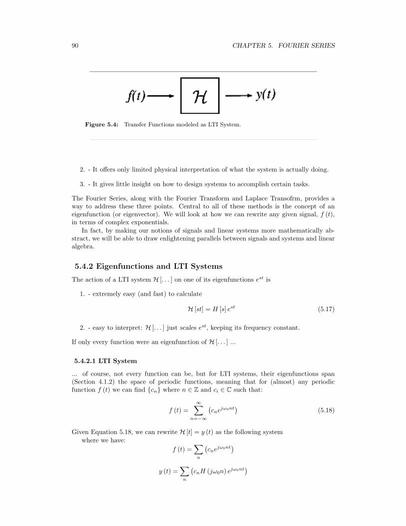
90 CHAPTER 5. FOURIER SERIES
Figure 5.4: Transfer Functions modeled as LTI System.
2. - It offers only limited physical interpretation of what the system is actually doing.
3. - It gives little insight on how to design systems to accomplish certain tasks.
The Fourier Series, along with the Fourier Transform and Laplace Transofrm, provides away to address these three points. Central to all of these methods is the concept of aneigenfunction (or eigenvector). We will look at how we can rewrite any given signal, f (t),in terms of complex exponentials.
In fact, by making our notions of signals and linear systems more mathematically ab-stract, we will be able to draw enlightening parallels between signals and systems and linearalgebra.
5.4.2 Eigenfunctions and LTI Systems
The action of a LTI system H [. . . ] on one of its eigenfunctions est is
1. - extremely easy (and fast) to calculate
H [st] = H [s] est (5.17)
2. - easy to interpret: H [. . . ] just scales est, keeping its frequency constant.
If only every function were an eigenfunction of H [. . . ] ...
5.4.2.1 LTI System
... of course, not every function can be, but for LTI systems, their eigenfunctions span(Section 4.1.2) the space of periodic functions, meaning that for (almost) any periodicfunction f (t) we can find cn where n ∈ Z and ci ∈ C such that:
f (t) =∞∑
n=−∞
(cne
jω0nt)
(5.18)
Given Equation 5.18, we can rewrite H [t] = y (t) as the following systemwhere we have:
f (t) =∑
n
(cne
jω0nt)
y (t) =∑
n
(cnH (jω0n) ejω0nt
)
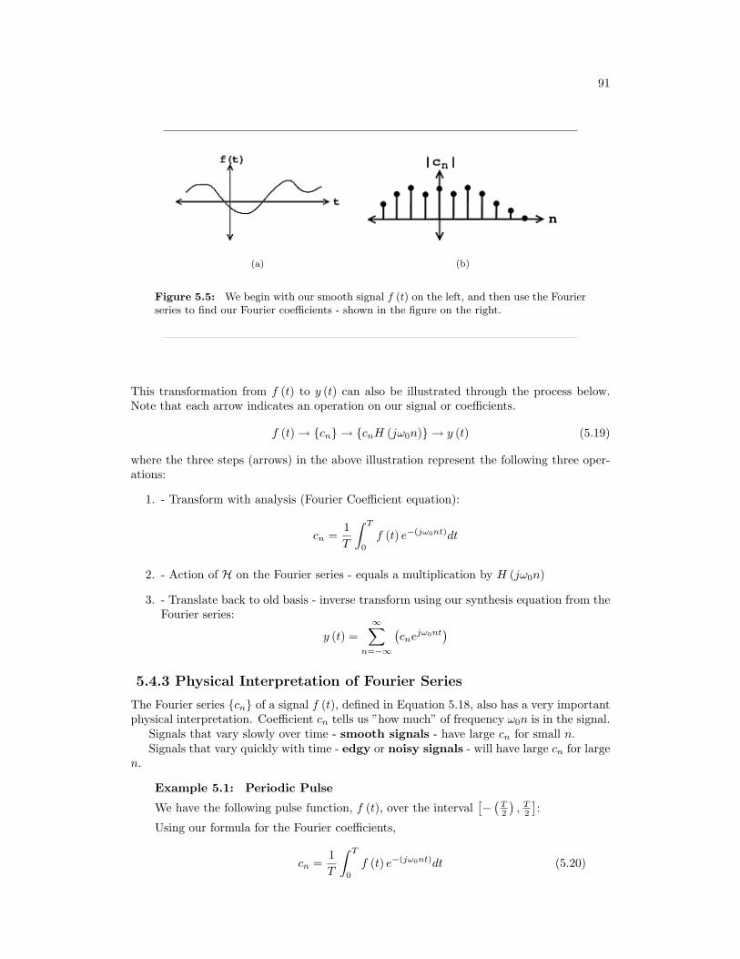
91
(a) (b)
Figure 5.5: We begin with our smooth signal f (t) on the left, and then use the Fourierseries to find our Fourier coefficients - shown in the figure on the right.
This transformation from f (t) to y (t) can also be illustrated through the process below.Note that each arrow indicates an operation on our signal or coefficients.
f (t) → cn → cnH (jω0n) → y (t) (5.19)
where the three steps (arrows) in the above illustration represent the following three oper-ations:
1. - Transform with analysis (Fourier Coefficient equation):
cn =1T
∫ T
0
f (t) e−(jω0nt)dt
2. - Action of H on the Fourier series - equals a multiplication by H (jω0n)
3. - Translate back to old basis - inverse transform using our synthesis equation from theFourier series:
y (t) =∞∑
n=−∞
(cne
jω0nt)
5.4.3 Physical Interpretation of Fourier Series
The Fourier series cn of a signal f (t), defined in Equation 5.18, also has a very importantphysical interpretation. Coefficient cn tells us ”how much” of frequency ω0n is in the signal.
Signals that vary slowly over time - smooth signals - have large cn for small n.Signals that vary quickly with time - edgy or noisy signals - will have large cn for large
n.
Example 5.1: Periodic Pulse
We have the following pulse function, f (t), over the interval[−(
T2
), T
2
]:
Using our formula for the Fourier coefficients,
cn =1T
∫ T
0
f (t) e−(jω0nt)dt (5.20)
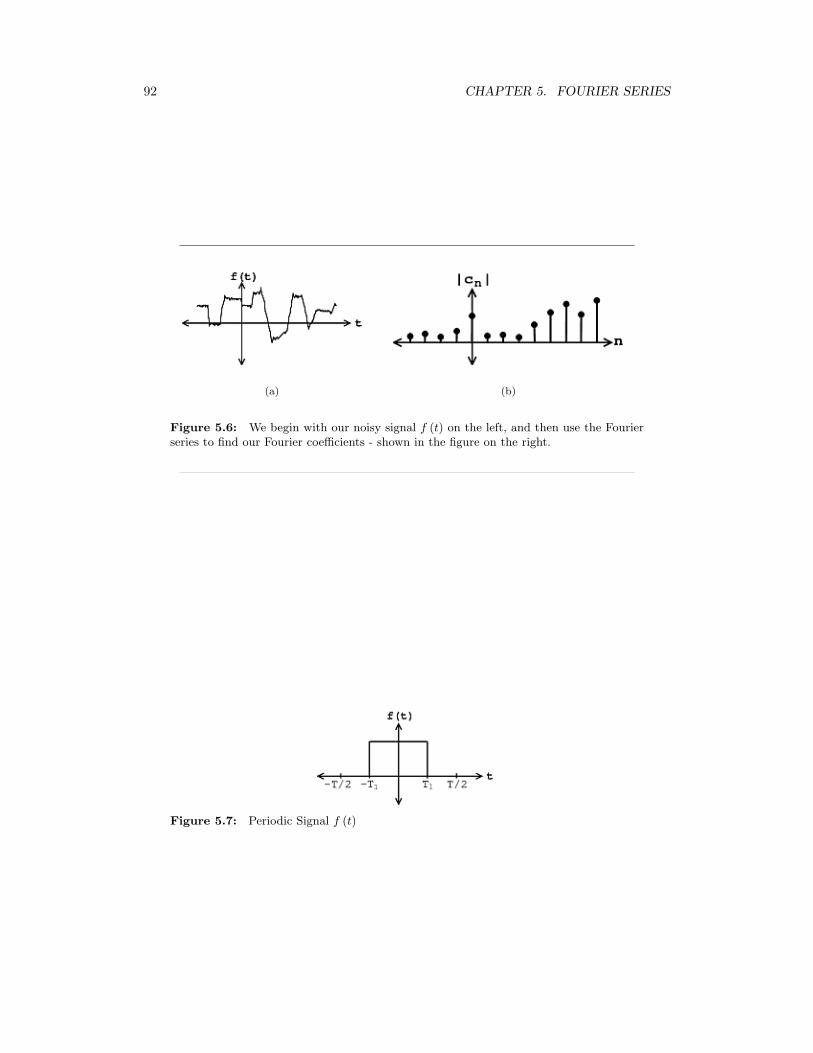
92 CHAPTER 5. FOURIER SERIES
(a) (b)
Figure 5.6: We begin with our noisy signal f (t) on the left, and then use the Fourierseries to find our Fourier coefficients - shown in the figure on the right.
Figure 5.7: Periodic Signal f (t)
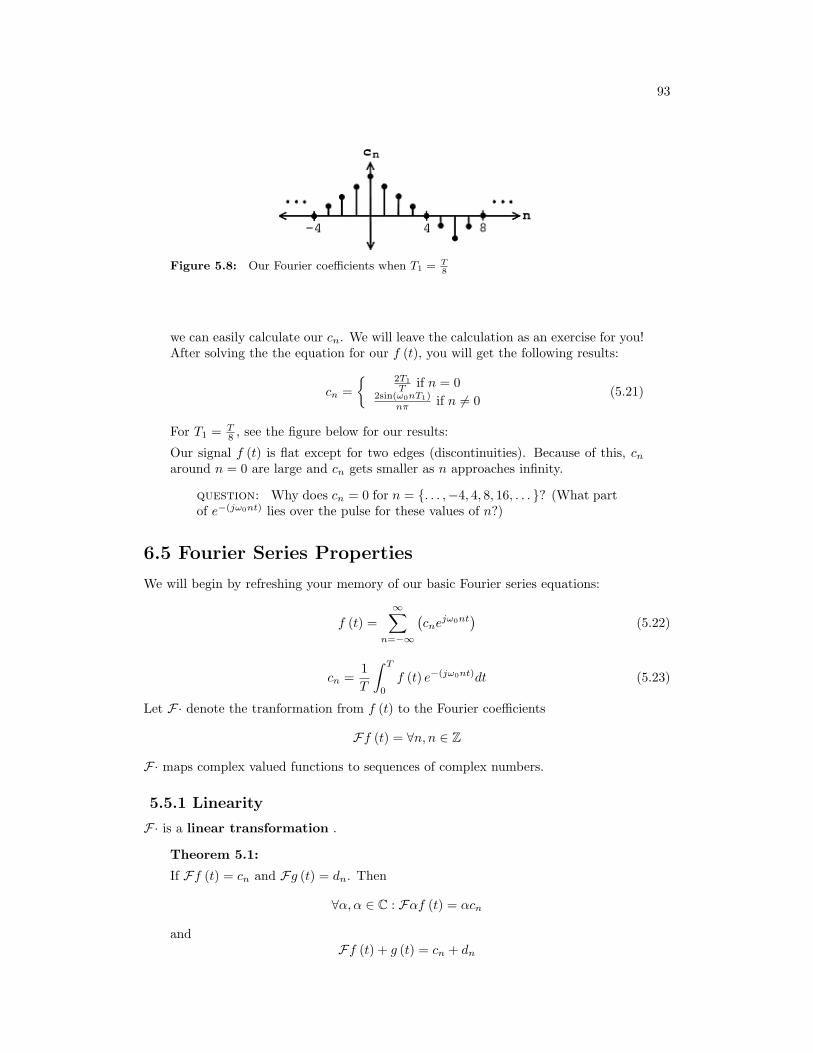
93
Figure 5.8: Our Fourier coefficients when T1 = T8
we can easily calculate our cn. We will leave the calculation as an exercise for you!After solving the the equation for our f (t), you will get the following results:
cn = 2T1
T if n = 02sin(ω0nT1)
nπ if n 6= 0(5.21)
For T1 = T8 , see the figure below for our results:
Our signal f (t) is flat except for two edges (discontinuities). Because of this, cnaround n = 0 are large and cn gets smaller as n approaches infinity.
question: Why does cn = 0 for n = . . . ,−4, 4, 8, 16, . . . ? (What partof e−(jω0nt) lies over the pulse for these values of n?)
6.5 Fourier Series Properties
We will begin by refreshing your memory of our basic Fourier series equations:
f (t) =∞∑
n=−∞
(cne
jω0nt)
(5.22)
cn =1T
∫ T
0
f (t) e−(jω0nt)dt (5.23)
Let F· denote the tranformation from f (t) to the Fourier coefficients
Ff (t) = ∀n, n ∈ Z
F· maps complex valued functions to sequences of complex numbers.
5.5.1 Linearity
F· is a linear transformation .
Theorem 5.1:
If Ff (t) = cn and Fg (t) = dn. Then
∀α, α ∈ C : Fαf (t) = αcn
andFf (t) + g (t) = cn + dn
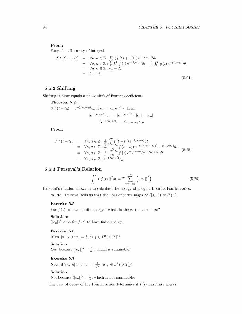
94 CHAPTER 5. FOURIER SERIES
Proof:Easy. Just linearety of integral.
Ff (t) + g (t) = ∀n, n ∈ Z :∫ T
0(f (t) + g (t)) e−(jω0nt)dt
= ∀n, n ∈ Z : 1T
∫ T
0f (t) e−(jω0nt)dt+ 1
T
∫ T
0g (t) e−(jω0nt)dt
= ∀n, n ∈ Z : cn + dn
= cn + dn
(5.24)
5.5.2 Shifting
Shifting in time equals a phase shift of Fourier coefficients
Theorem 5.2:
Ff (t− t0) = e−(jω0nt0)cn if cn = |cn|ej∠cn , then
|e−(jω0nt0)cn| = |e−(jω0nt0)||cn| = |cn|
∠e−(jω0t0n) = ∠cn − ω0t0n
Proof:
Ff (t− t0) = ∀n, n ∈ Z : 1T
∫ T
0f (t− t0) e−(jω0nt)dt
= ∀n, n ∈ Z : 1T
∫ T−t0−t0
f (t− t0) e−(jω0n(t−t0))e−(jω0nt0)dt
= ∀n, n ∈ Z : 1T
∫ T−t0−t0
f(t)e−(jω0nt)e−(jω0nt0)dt
= ∀n, n ∈ Z : e−(jω0nt)cn
(5.25)
5.5.3 Parseval’s Relation∫ T
0
(|f (t) |)2dt = T∞∑
n=−∞
((|cn|)2
)(5.26)
Parseval’s relation allows us to calculate the energy of a signal from its Fourier series.
note: Parseval tells us that the Fourier series maps L2 ([0, T ]) to l2 (Z).
Exercise 5.5:
For f (t) to have ”finite energy,” what do the cn do as n→∞?
Solution:(|cn|)2 <∞ for f (t) to have finite energy.
Exercise 5.6:
If ∀n, |n| > 0 : cn = 1n , is f ∈ L2 ([0, T ])?
Solution:Yes, because (|cn|)2 = 1
n2 , which is summable.
Exercise 5.7:
Now, if ∀n, |n| > 0 : cn = 1√n, is f ∈ L2 ([0, T ])?
Solution:No, because (|cn|)2 = 1
n , which is not summable.
The rate of decay of the Fourier series determines if f (t) has finite energy.
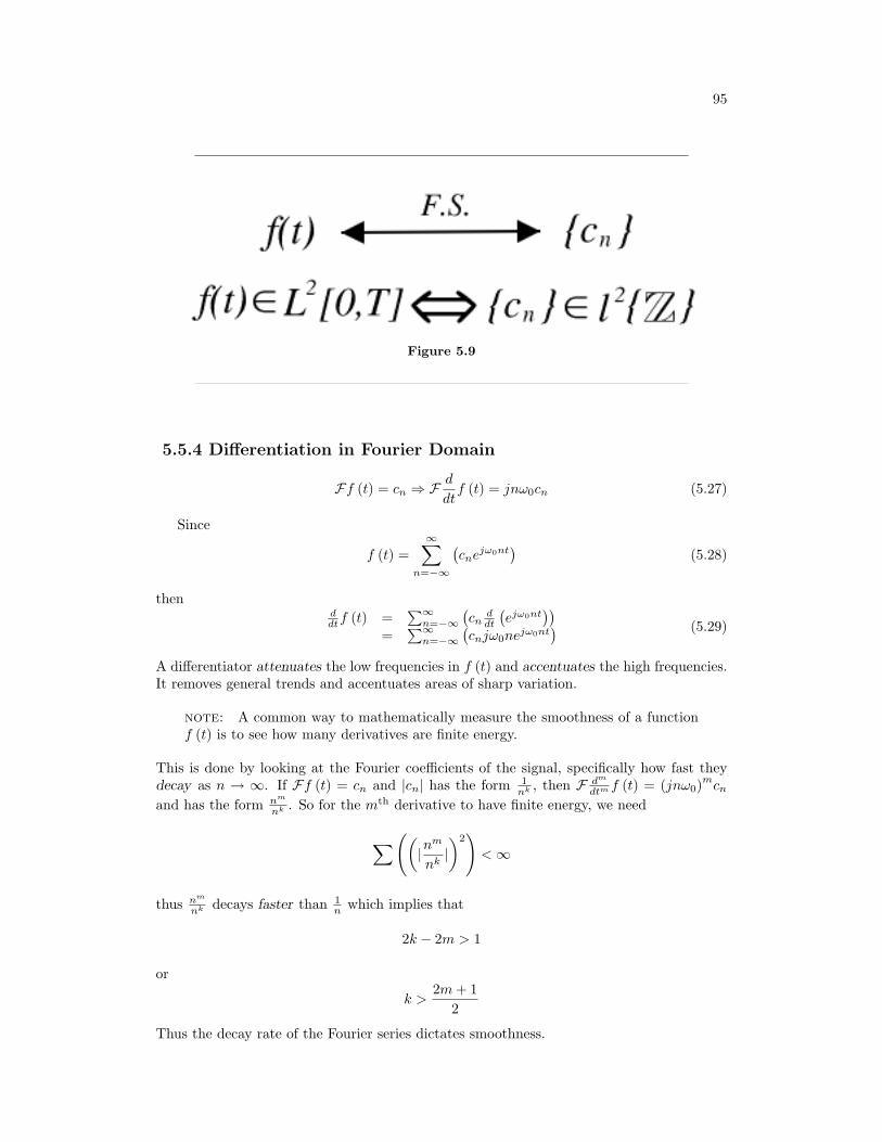
95
Figure 5.9
5.5.4 Differentiation in Fourier Domain
Ff (t) = cn ⇒ F d
dtf (t) = jnω0cn (5.27)
Since
f (t) =∞∑
n=−∞
(cne
jω0nt)
(5.28)
thenddtf (t) =
∑∞n=−∞
(cn
ddt
(ejω0nt
))=
∑∞n=−∞
(cnjω0ne
jω0nt) (5.29)
A differentiator attenuates the low frequencies in f (t) and accentuates the high frequencies.It removes general trends and accentuates areas of sharp variation.
note: A common way to mathematically measure the smoothness of a functionf (t) is to see how many derivatives are finite energy.
This is done by looking at the Fourier coefficients of the signal, specifically how fast theydecay as n → ∞. If Ff (t) = cn and |cn| has the form 1
nk , then F dm
dtm f (t) = (jnω0)mcn
and has the form nm
nk . So for the mth derivative to have finite energy, we need
∑((|n
m
nk|)2)<∞
thus nm
nk decays faster than 1n which implies that
2k − 2m > 1
or
k >2m+ 1
2
Thus the decay rate of the Fourier series dictates smoothness.

96 CHAPTER 5. FOURIER SERIES
5.5.5 Integration in the Fourier Domain
IfFf (t) = cn (5.30)
then
F∫ t
−∞f (τ) dτ =
1jω0n
cn (5.31)
note: If c0 6= 0, this expression doesn’t make sense.
Integration accentuates low frequencies and attenuates high frequencies. Integratorsbring out the general trends in signals and supress short term variation (which is noise inmany cases). Integrators are much nicer than differentiators.
5.5.6 Signal Multiplication
Given a signal f (t) with Fourier coefficients cn and a signal g (t) with Fourier coefficientsdn, we can define a new signal, y (t), where y (t) = f (t) g (t). We find that the FourierSeries representation of y (t), en, is such that en =
∑∞k=−∞ (ckdn−k). This is to say that
signal multiplication in the time domain is equivalent to discrete-time convolution in thefrequency domain. The proof of this is as follows
en = 1T
∫ T
0f (t) g (t) e−(jω0nt)dt
= 1T
∫ T
0
(∑∞k=−∞
(cke
jω0kt))g (t) e−(jω0nt)dt
=∑∞
k=−∞
(ck
(1T
∫ T
0g (t) e−(jω0(n−k)t)dt
))=
∑∞k=−∞ (ckdn−k)
(5.32)
6.6 Symmetry Properties of the Fourier Series
5.6.1 Symmetry Properties
5.6.1.1 Real Signals
Real signals have a conjugate symmetric Fourier series.
Theorem 5.3:
If f (t) is real it implies that f (t) = f (t)∗ (f (t)∗ is the complex conjugate off (t)), then cn = c−n
∗ which implies that Re (cn) = Re (c−n), i.e. the real part ofcn is even, and Im (cn) = − (Im (c−n)), i.e. the imaginary part of cn is odd. SeeFigure 5.10. It also implies that |cn| = |c−n|, i.e. that magnitude is even, and that∠cn = (∠− c−n), i.e. the phase is odd.
Proof:
c−n = 1T
∫ T
0f (t) ejω0ntdt
= ∀t, f (t) = f (t)∗ : 1T
∫ T
0f (t)∗e−(jω0nt)dt
∗
= 1T
∫ T
0f (t) e−(jω0nt)dt
∗
= cn∗
(5.33)

97
(a)
(b)
Figure 5.10: (a) Re (cn) = Re (c−n), and Im (cn) = − (Im (c−n)). (b) |cn| = |c−n|, and∠cn = (∠− c−n).
98 CHAPTER 5. FOURIER SERIES
5.6.1.2 Real and Even Signals
Real and even signals have real and even Fourier series.
Theorem 5.4:
If f (t) = f (t)∗ and f (t) = (f (−t)), i.e. the signal is real and even, then cn = c−n
and cn = cn∗.
Proof:
cn = 1T
∫ T2
−(T2 ) f (t) e−(jω0nt)dt
= 1T
∫ 0
−(T2 ) f (t) e−(jω0nt)dt+ 1
T
∫ T2
0f (t) e−(jω0nt)dt
= 1T
∫ T2
0f (−t) ejω0ntdt+ 1
T
∫ T2
0f (t) e−(jω0nt)dt
= 2T
∫ T2
0f (t) cos (ω0nt) dt
(5.34)
f (t) and cos (ω0nt) are both real which implies that cn is real. Also cos (ω0nt) =cos (− (ω0nt)) so cn = c−n. It is also easy to show that f (t) = 2
∑∞n=0 (cncos (ω0nt))
since f (t), cn, and cos (ω0nt) are all real and even.
5.6.1.3 Real and Odd Signals
Real and odd signals have Fourier Series that are odd and purely imaginary.
Theorem 5.5:
If f (t) = − (f (−t)) and f (t) = f (t)∗, i.e. the signal is real and odd, thencn = −c−n and cn = − (cn∗), i.e. cn is odd and purely imaginary.
Proof:Do it at home.
If f (t) is odd, then we can expand it in terms of sin (ω0nt):
f (t) =∞∑
n=1
(2cnsin (ω0nt))
5.6.2 Summary
In summary, we can find fe (t), an even function, and fo (t), an odd function, such that
f (t) = fe (t) + fo (t) (5.35)
which implies that, for any f (t), we can find an and bn such that
f (t) =∞∑
n=0
(ancos (ω0nt)) +∞∑
n=1
(bnsin (ω0nt)) (5.36)
Example 5.2: Triangle Wave
f (t) is real and odd.
cn =
4A
jπ2n2 if n = . . . ,−11,−7,−3, 1, 5, 9, . . . −(
4Ajπ2n2
)if n = . . . ,−9,−5,−1, 3, 7, 11, . . .
0 if n = . . . ,−4,−2, 0, 2, 4, . . .
Does cn = −c−n?
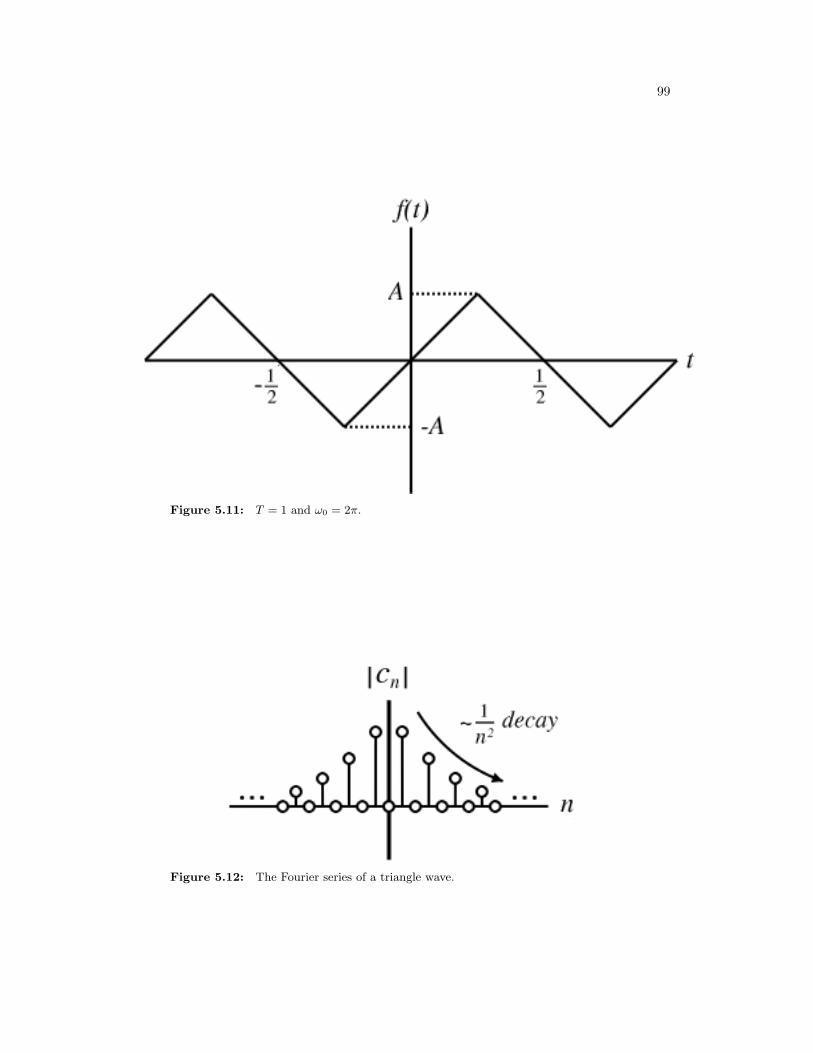
99
Figure 5.11: T = 1 and ω0 = 2π.
Figure 5.12: The Fourier series of a triangle wave.
100 CHAPTER 5. FOURIER SERIES
Note: We can often gather information about the smoothness of a signal byexamining its Fourier coefficients.
Take a look at the above examples. The pulse and sawtooth waves are not continuous andthere Fourier series’ fall off like 1
n . The triangle wave is continuous, but not differentiableand its Fourier series falls off like 1
n2 .The next 3 properties will give a better feel for this.
6.7 Circular Convolution Property of Fourier Series
5.7.1 Signal Circular Convolution
Given a signal f (t) with Fourier coefficients cn and a signal g (t) with Fourier coefficientsdn, we can define a new signal, v (t), where v (t) = (f (t) @@g (t)) We find that the FourierSeries representation of y (t), an, is such that an = cndn. (f (t) @@g (t)) is the circularconvolution of two periodic signals and is equivilent to the convolution over one interval,i.e. (f (t) @@g (t)) =
∫ T
0
∫ T
0f (τ) g (t− τ) dτdt.
note: Circular convolution in the time domain is equivalent to multiplication ofthe Fourier coefficients.
This is proved as follows
an = 1T
∫ T
0v (t) e−(jω0nt)dt
= 1T 2
∫ T
0
∫ T
0f (τ) g (t− τ) dτe−(jω0nt)dt
= 1T
∫ T
0f (τ)
(1T
∫ T
0g (t− τ) e−(jω0nt)dt
)dτ
= ∀ν, ν = t− τ : 1T
∫ T
0f (τ)
(1T
∫ T−τ
−τg (ν) e−(jω0(ν+τ))dν
)dτ
= 1T
∫ T
0f (τ)
(1T
∫ T−τ
−τg (ν) e−(jω0nν)dν
)e−(jω0nτ)dτ
= 1T
∫ T
0f (τ) dne
−(jω0nτ)dτ
= dn
(1T
∫ T
0f (τ) e−(jω0nτ)dτ
)= cndn
(5.37)
Example 5.3:
Take a look at a square pulse with a period, T1 = T4 :
For this signal
cn =
1T if n = 0
12
sin(π2 n)
π2 n otherwise
Exercise 5.8:
What signal has Fourier coefficients an = cn2 = 1
4
sin2(π2 n)
(π2 n)2 ?
Solution:
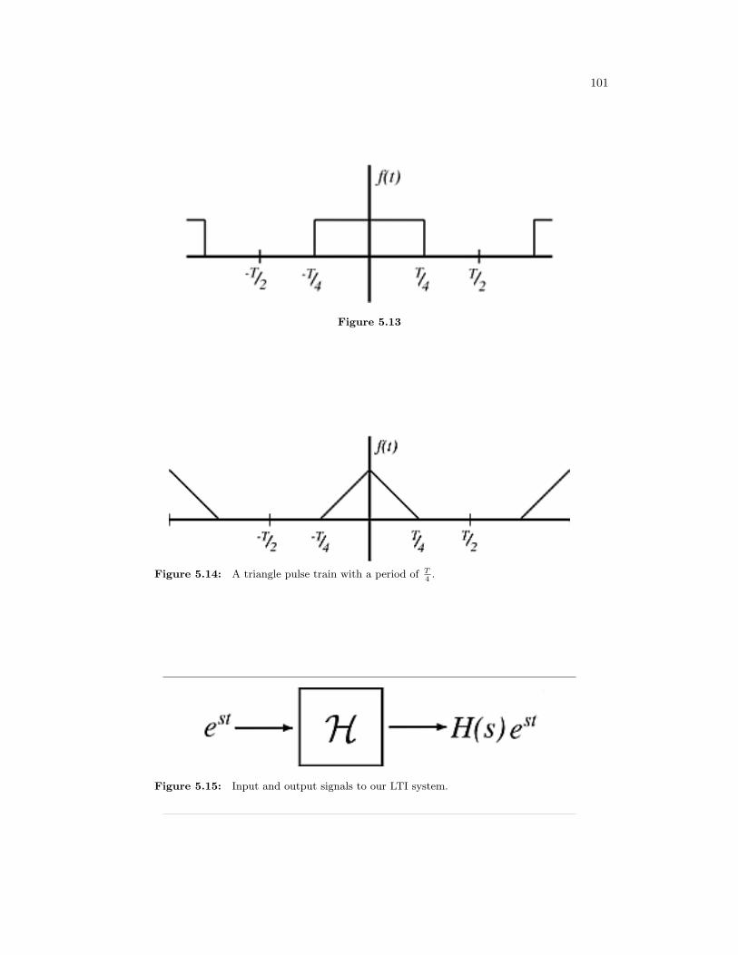
101
Figure 5.13
Figure 5.14: A triangle pulse train with a period of T4.
Figure 5.15: Input and output signals to our LTI system.
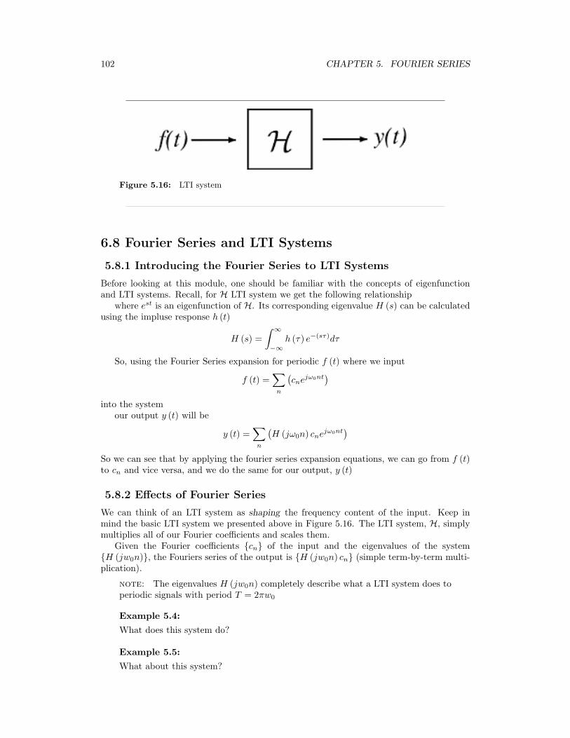
102 CHAPTER 5. FOURIER SERIES
Figure 5.16: LTI system
6.8 Fourier Series and LTI Systems
5.8.1 Introducing the Fourier Series to LTI Systems
Before looking at this module, one should be familiar with the concepts of eigenfunctionand LTI systems. Recall, for H LTI system we get the following relationship
where est is an eigenfunction of H. Its corresponding eigenvalue H (s) can be calculatedusing the impluse response h (t)
H (s) =∫ ∞
−∞h (τ) e−(sτ)dτ
So, using the Fourier Series expansion for periodic f (t) where we input
f (t) =∑
n
(cne
jω0nt)
into the systemour output y (t) will be
y (t) =∑
n
(H (jω0n) cnejω0nt
)So we can see that by applying the fourier series expansion equations, we can go from f (t)to cn and vice versa, and we do the same for our output, y (t)
5.8.2 Effects of Fourier Series
We can think of an LTI system as shaping the frequency content of the input. Keep inmind the basic LTI system we presented above in Figure 5.16. The LTI system, H, simplymultiplies all of our Fourier coefficients and scales them.
Given the Fourier coefficients cn of the input and the eigenvalues of the systemH (jw0n), the Fouriers series of the output is H (jw0n) cn (simple term-by-term multi-plication).
note: The eigenvalues H (jw0n) completely describe what a LTI system does toperiodic signals with period T = 2πw0
Example 5.4:
What does this system do?
Example 5.5:
What about this system?
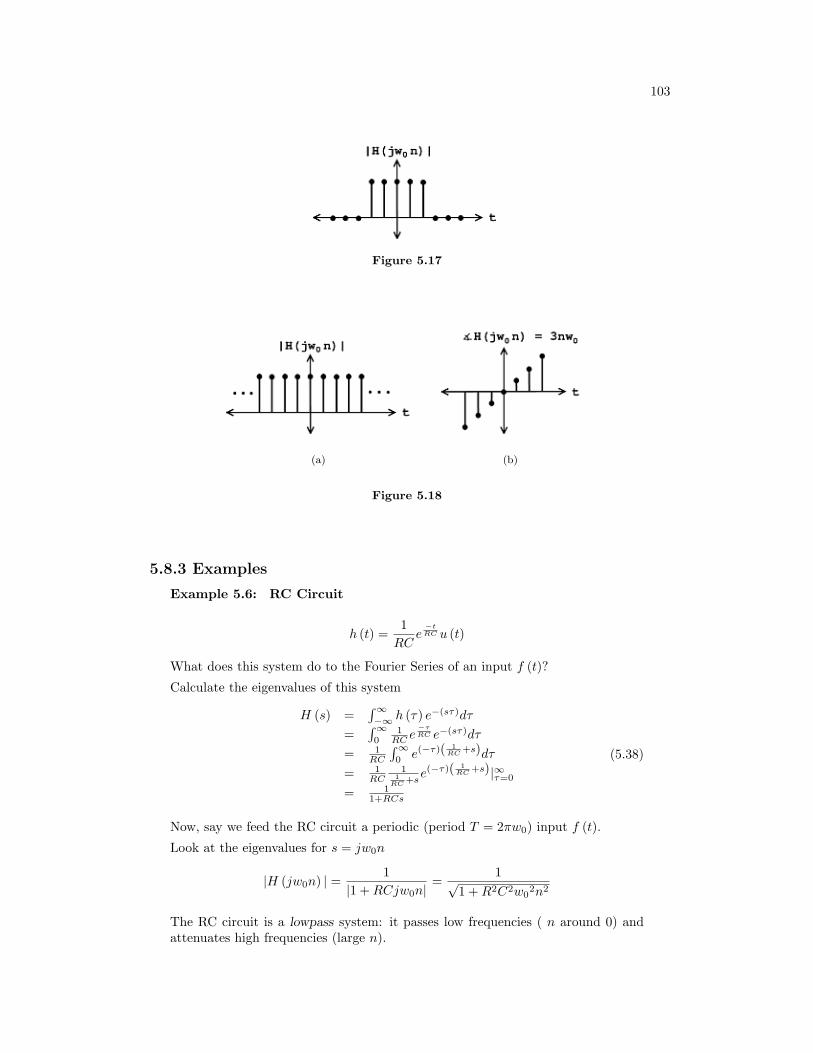
103
Figure 5.17
(a) (b)
Figure 5.18
5.8.3 Examples
Example 5.6: RC Circuit
h (t) =1RC
e−tRC u (t)
What does this system do to the Fourier Series of an input f (t)?
Calculate the eigenvalues of this system
H (s) =∫∞−∞ h (τ) e−(sτ)dτ
=∫∞0
1RC e
−τRC e−(sτ)dτ
= 1RC
∫∞0e(−τ)( 1
RC +s)dτ= 1
RC1
1RC +s
e(−τ)( 1RC +s)|∞τ=0
= 11+RCs
(5.38)
Now, say we feed the RC circuit a periodic (period T = 2πw0) input f (t).
Look at the eigenvalues for s = jw0n
|H (jw0n) | = 1|1 +RCjw0n|
=1√
1 +R2C2w02n2
The RC circuit is a lowpass system: it passes low frequencies ( n around 0) andattenuates high frequencies (large n).
104 CHAPTER 5. FOURIER SERIES
Example 5.7: Square pulse wave througth RC circuit
•- Input Signal: Taking the fourier series of f (t)
cn =12
sin(
π2n)
π2n
1t at n = 0
•- System: eigenvalues
H (jw0n) =1
1 + jRCw0n
•- Output Signal: Taking the fourier series of y (t)
dn = H (jw0n) cn =1
1 + jRCw0n
12
sin(
π2n)
π2n
dn =1
1 + jRCw0n
12
sin(
π2n)
π2n
y (t) =∑(
dnejw0nt
)What can we infer about y (t) from dn?
1.- Is y (t) real?
2.- Is y (t) even symmetric? odd symmetric?
3.- Qualitatively, what does y (t) look like? Is it ”smoother” than f (t)? (decayrete of dn vs. cn)
dn =1
1 + jRCw0n
12
sin(
π2n)
π2n
|dn| =1√
1 + (RCw0)2n2
12
sin(
π2n)
π2n
6.9 Convergence of Fourier Series
5.9.1 Introduction
Before looking at this module, hopefully you have become fully convinced of the fact thatany periodic (pg ??) function, f (t), can be represented as a sum of complex sinusoids.If you are not, then try looking back at eigen-stuff in a nutshell or eigenfunctions of LTIsystems. We have shown that we can represent a signal as the sum of exponentials throughthe Fourier Series equations below:
f (t) =∑
n
(cne
jω0nt)
(5.39)
cn =1T
∫ T
0
f (t) e−(jω0nt)dt (5.40)
105
Joseph Fourier2 insisted that these equations were true, but could not prove it. Lagrangepublicly ridiculed Fourier, and said that only continuous functions can be represented byEquation 5.39 (indeed he proved that Equation 5.39 holds for continuous-time functions).However, we know now that the real truth lies in between Fourier and Lagrange’s positions.
5.9.2 Understanding the Truth
Formulating our question mathematically, let
f ′N (t) =N∑
n=−N
(cne
jω0nt)
where cn equals the Fourier coefficients of f (t) (see Equation 5.40).f ′N (t) is a ”partial reconstruction” of f (t) using the first 2N+1 Fourier coefficients.
f ′N (t) approximates f (t), with the approximation getting better and better as N getslarge. Therefore, we can think of the set ∀N,N = 0, 1, . . . : f ′N (t) as a sequence offunctions , each one approximating f (t) better than the one before.
The question is, does this sequence converge to f (t)? Does f ′N (t) → f (t) as N → ∞?We will try to answer this question by thinking about convergence in two different ways:
1. - Looking at the energy of the error signal:
eN (t) = f (t)− f ′N (t)
2. - Looking at limN→∞
f ′N (t) at each point and comparing to f (t).
5.9.2.1 Approach #1
Let eN (t) be the difference (i.e. error) between the signal f (t) and its partial reconstructionf ′N (t)
eN (t) = f (t)− f ′N (t) (5.41)
If f (t) ∈ L2 ([0, T ]) (finite energy), then the energy of eN (t) → 0 as N →∞ is∫ T
0
(|eN (t) |)2dt =∫ T
0
(f (t)− f ′N (t))2dt→ 0 (5.42)
We can prove this equation using Parseval’s relation:
limN→∞
∫ T
0
(|f (t)− f ′N (t) |)2dt = limN→∞
∞∑N=−∞
((|Fnf (t)−Fnf
′N (t) |)2
)= lim
N→∞
∑|n|>N
((|cn|)2
)= 0
where the last equation before zero is the tail sum of the Fourier Series, which approacheszero because f (t) ∈ L2 ([0, T ]). Since physical systems respond to energy, the Fourier Seriesprovides an adequate representation for all f (t) ∈ L2 ([0, T ]) equaling finite energy over oneperiod.
5.9.2.2 Approach #2
The fact that eN → 0 says nothing about f (t) and limN→∞
f ′N (t) being equal at a given point.
Take the two functions graphed below for example:2http://www-groups.dcs.st-and.ac.uk/∼history/Mathematicians/Fourier.html
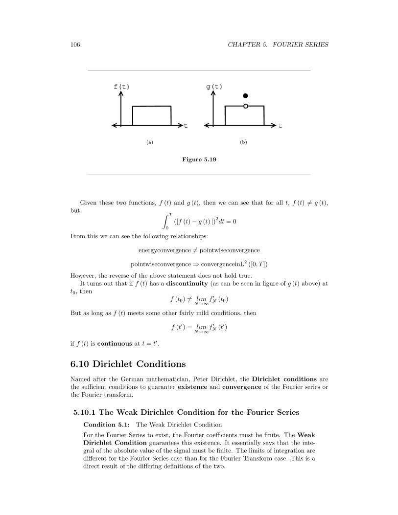
106 CHAPTER 5. FOURIER SERIES
(a) (b)
Figure 5.19
Given these two functions, f (t) and g (t), then we can see that for all t, f (t) 6= g (t),but ∫ T
0
(|f (t)− g (t) |)2dt = 0
From this we can see the following relationships:
energyconvergence 6= pointwiseconvergence
pointwiseconvergence ⇒ convergenceinL2 ([0, T ])
However, the reverse of the above statement does not hold true.It turns out that if f (t) has a discontinuity (as can be seen in figure of g (t) above) at
t0, thenf (t0) 6= lim
N→∞f ′N (t0)
But as long as f (t) meets some other fairly mild conditions, then
f (t′) = limN→∞
f ′N (t′)
if f (t) is continuous at t = t′.
6.10 Dirichlet Conditions
Named after the German mathematician, Peter Dirichlet, the Dirichlet conditions arethe sufficient conditions to guarantee existence and convergence of the Fourier series orthe Fourier transform.
5.10.1 The Weak Dirichlet Condition for the Fourier Series
Condition 5.1: The Weak Dirichlet Condition
For the Fourier Series to exist, the Fourier coefficients must be finite. The WeakDirichlet Condition guarantees this existence. It essentially says that the inte-gral of the absolute value of the signal must be finite. The limits of integration aredifferent for the Fourier Series case than for the Fourier Transform case. This is adirect result of the differing definitions of the two.
107
Proof:The Fourier Series exists (the coefficients are finite) if
Weak Dirichlet Condition for the Fourier Series∫ T
0
|f (t) |dt <∞ (5.43)
This can be shown from the intial condition that the Fourier Series coefficients befinite.
|cn| = | 1T
∫ T
0
f (t) e−(jω0nt)dt| ≤ 1T
∫ T
0
|f (t) ||e−(jω0nt)|dt (5.44)
Remembering our complex exponentials, we know that in the above equation|e−(jω0nt)| = 1, which gives us
1T
∫ T
0
|f (t) |dt =1T
∫ T
0
|f (t) |dt (5.45)
<∞ (5.46)
note: If we have the function:
∀t, 0 < t ≤ T : f (t) =1t
then you should note that this functions fails the above condition.
5.10.1.1 The Weak Dirichlet Condition for the Fourier Transform
Condition 5.2:
The Fourier Transform exists if
Weak Dirichlet Condition for the Fourier Transform∫ ∞
−∞|f (t) |dt <∞ (5.47)
This can be derived the same way the weak Dirichlet for the Fourier Series wasderived, by beginning with the definition and showing that the Fourier Transformmust be less than infinity everywhere.
5.10.2 The Strong Dirichlet Conditions
The Fourier Transform exists if the signal has a finite number of discontinuities and afinite number of maxima and minima . For the Fourier Series to exist, the following twoconditions must be satisfied (along with the Weak Dirichlet Condition):
1. - In one period, f (t) has only a finite number of minima and maxima.
2. - In one period, f (t) has only a finite number of discontinuities and each one is finite.
These are what we refer to as the Strong Dirichlet Conditions . In theory we can thinkof signals that violate these conditions, sin (logt) for instance. However, it is not possible tocreate a signal that violates these conditions in a lab. Therefore, any real-world signal willhave a Fourier representation.
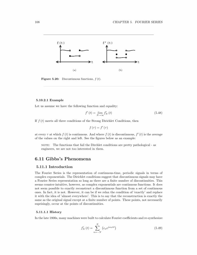
108 CHAPTER 5. FOURIER SERIES
(a) (b)
Figure 5.20: Discontinuous functions, f (t).
5.10.2.1 Example
Let us assume we have the following function and equality:
f ′ (t) = limN→∞
f ′N (t) (5.48)
If f (t) meets all three conditions of the Strong Dirichlet Conditions, then
f (τ) = f ′ (τ)
at every τ at which f (t) is continuous. And where f (t) is discontinuous, f ′ (t) is the averageof the values on the right and left. See the figures below as an example:
note: The functions that fail the Dirchlet conditions are pretty pathological - asengineers, we are not too interested in them.
6.11 Gibbs’s Phenomena
5.11.1 Introduction
The Fourier Series is the representation of continuous-time, periodic signals in terms ofcomplex exponentials. The Dirichlet conditions suggest that discontinuous signals may havea Fourier Series representation so long as there are a finite number of discontinuities. Thisseems counter-intuitive, however, as complex exponentials are continuous functions. It doesnot seem possible to exactly reconstruct a discontinuous function from a set of continuousones. In fact, it is not. However, it can be if we relax the condition of ’exactly’ and replaceit with the idea of ’almost everywhere’. This is to say that the reconstruction is exactly thesame as the original signal except at a finite number of points. These points, not necessarilysuprisingly, occur at the points of discontinuities.
5.11.1.1 History
In the late 1800s, many machines were built to calculate Fourier coefficients and re-synthesize:
f ′N (t) =N∑
n=−N
(cne
jω0nt)
(5.49)
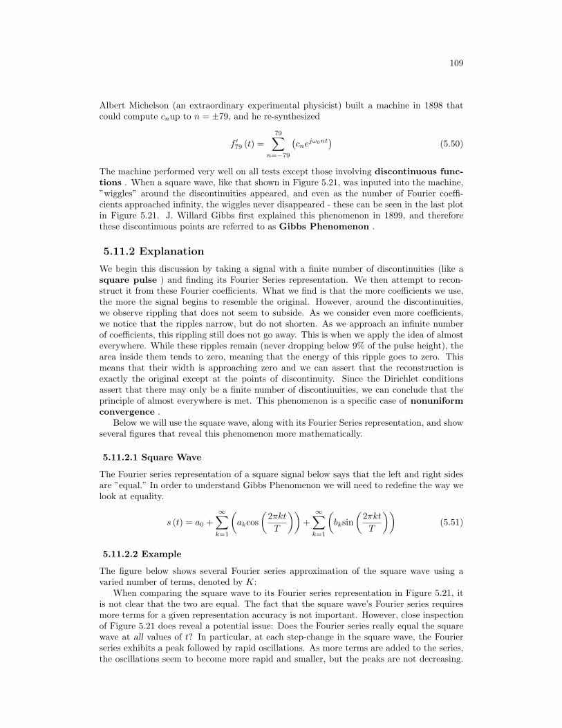
109
Albert Michelson (an extraordinary experimental physicist) built a machine in 1898 thatcould compute cnup to n = ±79, and he re-synthesized
f ′79 (t) =79∑
n=−79
(cne
jω0nt)
(5.50)
The machine performed very well on all tests except those involving discontinuous func-tions . When a square wave, like that shown in Figure 5.21, was inputed into the machine,”wiggles” around the discontinuities appeared, and even as the number of Fourier coeffi-cients approached infinity, the wiggles never disappeared - these can be seen in the last plotin Figure 5.21. J. Willard Gibbs first explained this phenomenon in 1899, and thereforethese discontinuous points are referred to as Gibbs Phenomenon .
5.11.2 Explanation
We begin this discussion by taking a signal with a finite number of discontinuities (like asquare pulse ) and finding its Fourier Series representation. We then attempt to recon-struct it from these Fourier coefficients. What we find is that the more coefficients we use,the more the signal begins to resemble the original. However, around the discontinuities,we observe rippling that does not seem to subside. As we consider even more coefficients,we notice that the ripples narrow, but do not shorten. As we approach an infinite numberof coefficients, this rippling still does not go away. This is when we apply the idea of almosteverywhere. While these ripples remain (never dropping below 9% of the pulse height), thearea inside them tends to zero, meaning that the energy of this ripple goes to zero. Thismeans that their width is approaching zero and we can assert that the reconstruction isexactly the original except at the points of discontinuity. Since the Dirichlet conditionsassert that there may only be a finite number of discontinuities, we can conclude that theprinciple of almost everywhere is met. This phenomenon is a specific case of nonuniformconvergence .
Below we will use the square wave, along with its Fourier Series representation, and showseveral figures that reveal this phenomenon more mathematically.
5.11.2.1 Square Wave
The Fourier series representation of a square signal below says that the left and right sidesare ”equal.” In order to understand Gibbs Phenomenon we will need to redefine the way welook at equality.
s (t) = a0 +∞∑
k=1
(akcos
(2πktT
))+
∞∑k=1
(bksin
(2πktT
))(5.51)
5.11.2.2 Example
The figure below shows several Fourier series approximation of the square wave using avaried number of terms, denoted by K:
When comparing the square wave to its Fourier series representation in Figure 5.21, itis not clear that the two are equal. The fact that the square wave’s Fourier series requiresmore terms for a given representation accuracy is not important. However, close inspectionof Figure 5.21 does reveal a potential issue: Does the Fourier series really equal the squarewave at all values of t? In particular, at each step-change in the square wave, the Fourierseries exhibits a peak followed by rapid oscillations. As more terms are added to the series,the oscillations seem to become more rapid and smaller, but the peaks are not decreasing.
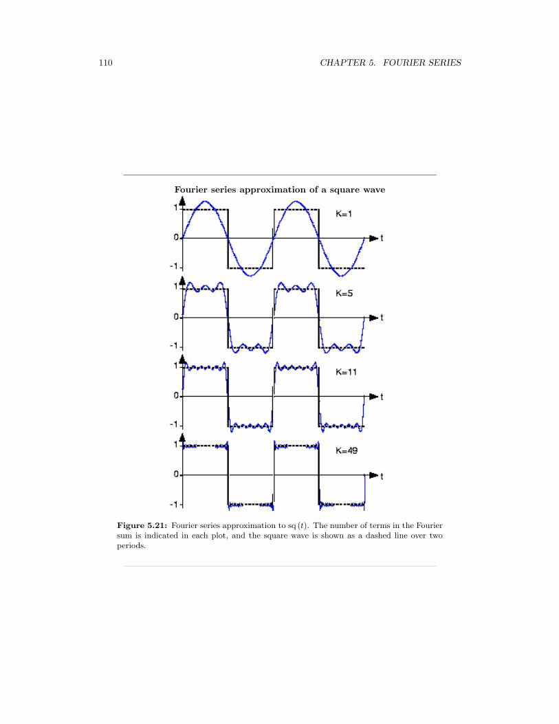
110 CHAPTER 5. FOURIER SERIES
Fourier series approximation of a square wave
Figure 5.21: Fourier series approximation to sq (t). The number of terms in the Fouriersum is indicated in each plot, and the square wave is shown as a dashed line over twoperiods.
111
Consider this mathematical question intuitively: Can a discontinuous function, like thesquare wave, be expressed as a sum, even an infinite one, of continuous ones? One should atleast be suspicious, and in fact, it can’t be thus expressed. This issue brought Fourier3 muchcriticism from the French Academy of Science (Laplace, Legendre, and Lagrange comprisedthe review committee) for several years after its presentation on 1807. It was not resolvedfor also a century, and its resolution is interesting and important to understand from apractical viewpoint.
The extraneous peaks in the square wave’s Fourier series never disappear; they aretermed Gibb’s phenomenon after the American physicist Josiah Willard Gibbs. Theyoccur whenever the signal is discontinuous, and will always be present whenever the signalhas jumps.
5.11.2.3 Redefine Equality
Let’s return to the question of equality; how can the equal sign in the definition of theFourier series (pg ??) be justified? The partial answer is that pointwise–each and everyvalue of t–equality is not guaranteed. What mathematicians later in the nineteenth centuryshowed was that the rms error of the Fourier series was always zero.
limK→∞
rms (εK) = 0 (5.52)
What this means is that the difference between an actual signal and its Fourier seriesrepresentation may not be zero, but the square of this quantity has zero integral! It isthrough the eyes of the rms value that we define equality: Two signals s1 (t), s2 (t) aresaid to be equal in the mean square if rms (s1 − s2) = 0. These signals are said to beequal pointwise if s1 (t) = s2 (t) for all values of t. For Fourier series, Gibb’s phenomenonpeaks have finite height and zero width: The error differs from zero only at isolated points–whenever the periodic signal contains discontinuities–and equals about 9% of the size of thediscontinuity. The value of a function at a finite set of points does not affect its integral.This effect underlies the reason why defining the value of a discontinuous function at itsdiscontinuity is meaningless. Whatever you pick for a value has no practical relevance foreither the signal’s spectrum or for how a system responds to the signal. The Fourier seriesvalue ”at” the discontinuity is the average of the values on either side of the jump.
6.12 Fourier Series Wrap-Up
Below we will highlight some of the most important concepts about the Fourier Series andour understanding of it through eigenfunctions and eigenvalues. Hopefully you are familiarwith all of this material, so this document will simply serve as a refrehser, but if not, thenrefer to the many links below for more information on the various ideas and topics.
1. - We can represent a periodic function (or a function on an interval) f (t) as a combi-nation of complex exponentials:
f (t) =∞∑
n=−∞
(cne
jω0nt)
(5.53)
cn =1T
∫ T
0
f (t) e−(jω0nt)dt (5.54)
Where the fourier coefficints, cn, approximately equal how much of frequency ωon isin the signal.
3http://www-groups.dcs.st-and.ac.uk/∼history/Mathematicians/Fourier.html
112 CHAPTER 5. FOURIER SERIES
2. - Since ejω0nt are eigenfunctions of LTI systems, we can interpret the action of a systemon a signal in terms of its eigenvalues:
H (jω0n) =∫ ∞
−∞h (t) e−(jω0nt)dt (5.55)
• - |H (jω0n) | is large ⇒ system accentuates frequency ω0n
• - |H (jω0n) | is small ⇒ system attenuates frequency ω0n
3. - In addition, the cn of a periodic function f (t) can tell us about:
• - symmetries in f (t)
• - smoothness of f (t), where smoothness can be interpretted as the decay rate of|cn|.
4. - We can approximate a function by re-synthesizing using only some of the Fouriercoefficients (truncating the F.S.)
f ′N (t) =∑
n≤|N |
(cne
jω0nt)
(5.56)
This approximation works well where f (t) is continuous, but not so well where f (t)is discontinuous. This idea is explained by Gibb’s Phenomena.
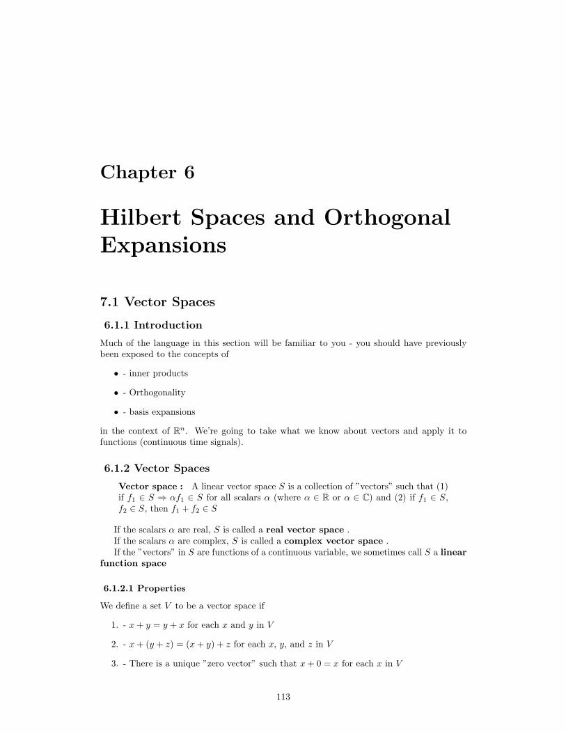
Chapter 6
Hilbert Spaces and OrthogonalExpansions
7.1 Vector Spaces
6.1.1 Introduction
Much of the language in this section will be familiar to you - you should have previouslybeen exposed to the concepts of
• - inner products
• - Orthogonality
• - basis expansions
in the context of Rn. We’re going to take what we know about vectors and apply it tofunctions (continuous time signals).
6.1.2 Vector Spaces
Vector space : A linear vector space S is a collection of ”vectors” such that (1)if f1 ∈ S ⇒ αf1 ∈ S for all scalars α (where α ∈ R or α ∈ C) and (2) if f1 ∈ S,f2 ∈ S, then f1 + f2 ∈ S
If the scalars α are real, S is called a real vector space .If the scalars α are complex, S is called a complex vector space .If the ”vectors” in S are functions of a continuous variable, we sometimes call S a linear
function space
6.1.2.1 Properties
We define a set V to be a vector space if
1. - x+ y = y + x for each x and y in V
2. - x+ (y + z) = (x+ y) + z for each x, y, and z in V
3. - There is a unique ”zero vector” such that x+ 0 = x for each x in V
113
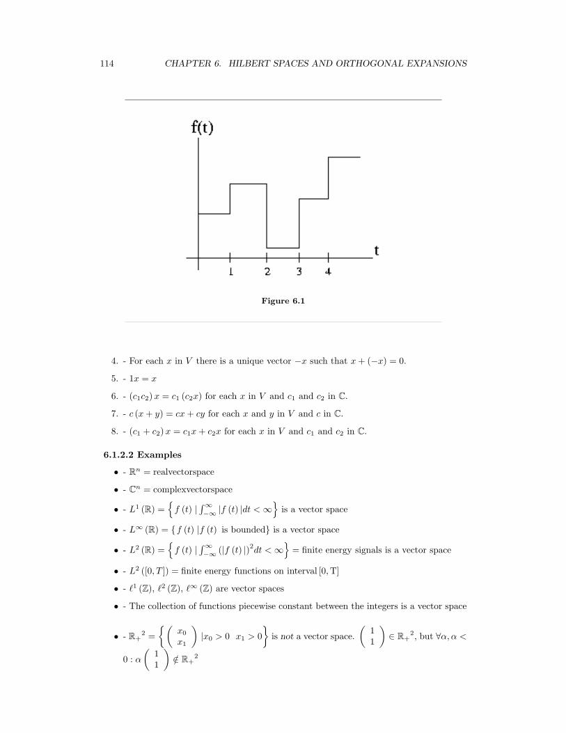
114 CHAPTER 6. HILBERT SPACES AND ORTHOGONAL EXPANSIONS
Figure 6.1
4. - For each x in V there is a unique vector −x such that x+ (−x) = 0.
5. - 1x = x
6. - (c1c2)x = c1 (c2x) for each x in V and c1 and c2 in C.
7. - c (x+ y) = cx+ cy for each x and y in V and c in C.
8. - (c1 + c2)x = c1x+ c2x for each x in V and c1 and c2 in C.
6.1.2.2 Examples
• - Rn = realvectorspace
• - Cn = complexvectorspace
• - L1 (R) =f (t) |
∫∞−∞ |f (t) |dt <∞
is a vector space
• - L∞ (R) = f (t) |f (t) is bounded is a vector space
• - L2 (R) =f (t) |
∫∞−∞ (|f (t) |)2dt <∞
= finite energy signals is a vector space
• - L2 ([0, T ]) = finite energy functions on interval [0,T]
• - `1 (Z), `2 (Z), `∞ (Z) are vector spaces
• - The collection of functions piecewise constant between the integers is a vector space
• - R+2 =
(x0
x1
)|x0 > 0 x1 > 0
is not a vector space.
(11
)∈ R+
2, but ∀α, α <
0 : α(
11
)/∈ R+
2
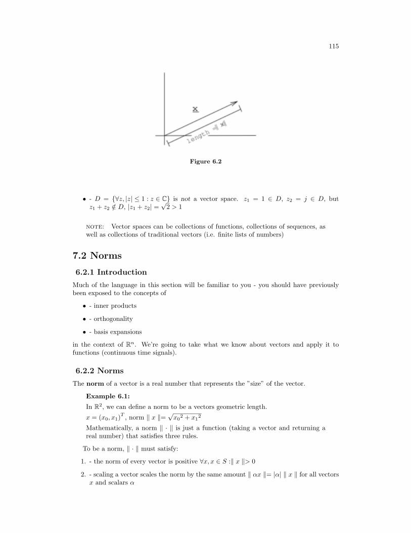
115
Figure 6.2
• - D = ∀z, |z| ≤ 1 : z ∈ C is not a vector space. z1 = 1 ∈ D, z2 = j ∈ D, butz1 + z2 /∈ D, |z1 + z2| =
√2 > 1
note: Vector spaces can be collections of functions, collections of sequences, aswell as collections of traditional vectors (i.e. finite lists of numbers)
7.2 Norms
6.2.1 Introduction
Much of the language in this section will be familiar to you - you should have previouslybeen exposed to the concepts of
• - inner products
• - orthogonality
• - basis expansions
in the context of Rn. We’re going to take what we know about vectors and apply it tofunctions (continuous time signals).
6.2.2 Norms
The norm of a vector is a real number that represents the ”size” of the vector.
Example 6.1:
In R2, we can define a norm to be a vectors geometric length.
x = (x0, x1)T , norm ‖ x ‖=
√x0
2 + x12
Mathematically, a norm ‖ · ‖ is just a function (taking a vector and returning areal number) that satisfies three rules.
To be a norm, ‖ · ‖ must satisfy:
1. - the norm of every vector is positive ∀x, x ∈ S :‖ x ‖> 0
2. - scaling a vector scales the norm by the same amount ‖ αx ‖= |α| ‖ x ‖ for all vectorsx and scalars α
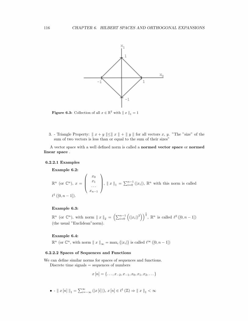
116 CHAPTER 6. HILBERT SPACES AND ORTHOGONAL EXPANSIONS
Figure 6.3: Collection of all x ∈ R2 with ‖ x ‖1 = 1
3. - Triangle Property: ‖ x + y ‖≤‖ x ‖ + ‖ y ‖ for all vectors x, y. ”The ”size” of thesum of two vectors is less than or equal to the sum of their sizes”
A vector space with a well defined norm is called a normed vector space or normedlinear space .
6.2.2.1 Examples
Example 6.2:
Rn (or Cn), x =
x0
x1
. . .xn−1
, ‖ x ‖1 =∑n−1
i=0 (|xi|), Rn with this norm is called
`1 ([0, n− 1]).
Example 6.3:
Rn (or Cn), with norm ‖ x ‖2 =(∑n−1
i=0
((|xi|)2
)) 12, Rn is called `2 ([0, n− 1])
(the usual ”Euclidean”norm).
Example 6.4:
Rn (or Cn, with norm ‖ x ‖∞ = maxi |xi| is called `∞ ([0, n− 1])
6.2.2.2 Spaces of Sequences and Functions
We can define similar norms for spaces of sequences and functions.Discrete time signals = sequences of numbers
x [n] = . . . , x−2, x−1, x0, x1, x2, . . .
• - ‖ x [n] ‖1 =∑∞
i=−∞ (|x [i] |), x [n] ∈ `1 (Z) ⇒ ‖ x ‖1 <∞
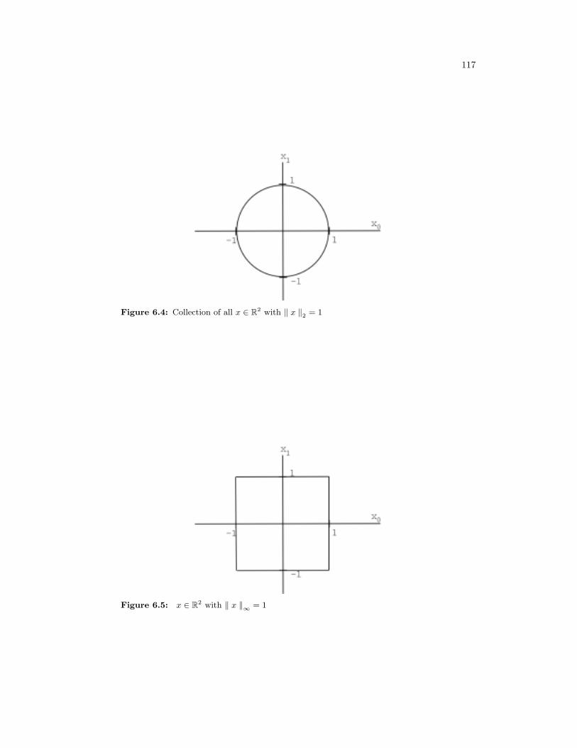
117
Figure 6.4: Collection of all x ∈ R2 with ‖ x ‖2 = 1
Figure 6.5: x ∈ R2 with ‖ x ‖∞ = 1
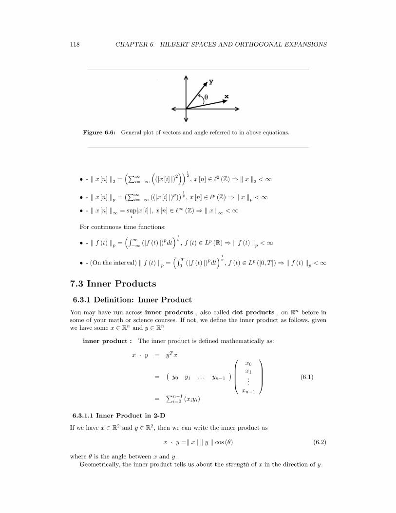
118 CHAPTER 6. HILBERT SPACES AND ORTHOGONAL EXPANSIONS
Figure 6.6: General plot of vectors and angle referred to in above equations.
• - ‖ x [n] ‖2 =(∑∞
i=−∞
((|x [i] |)2
)) 12, x [n] ∈ `2 (Z) ⇒ ‖ x ‖2 <∞
• - ‖ x [n] ‖p =(∑∞
i=−∞ ((|x [i] |)p)) 1
p , x [n] ∈ `p (Z) ⇒ ‖ x ‖p <∞
• - ‖ x [n] ‖∞ = supi|x [i] |, x [n] ∈ `∞ (Z) ⇒ ‖ x ‖∞ <∞
For continuous time functions:
• - ‖ f (t) ‖p =(∫∞
−∞ (|f (t) |)pdt) 1
p
, f (t) ∈ Lp (R) ⇒ ‖ f (t) ‖p <∞
• - (On the interval) ‖ f (t) ‖p =(∫ T
0(|f (t) |)p
dt) 1
p
, f (t) ∈ Lp ([0, T ]) ⇒ ‖ f (t) ‖p <∞
7.3 Inner Products
6.3.1 Definition: Inner Product
You may have run across inner prodcuts , also called dot products , on Rn before insome of your math or science courses. If not, we define the inner product as follows, givenwe have some x ∈ Rn and y ∈ Rn
inner product : The inner product is defined mathematically as:
x · y = yTx
=(y0 y1 . . . yn−1
)
x0
x1
...xn−1
=
∑n−1i=0 (xiyi)
(6.1)
6.3.1.1 Inner Product in 2-D
If we have x ∈ R2 and y ∈ R2, then we can write the inner product as
x · y =‖ x ‖‖ y ‖ cos (θ) (6.2)
where θ is the angle between x and y.Geometrically, the inner product tells us about the strength of x in the direction of y.
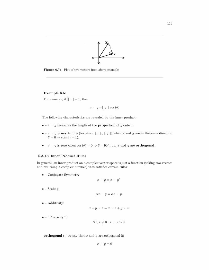
119
Figure 6.7: Plot of two vectors from above example.
Example 6.5:
For example, if ‖ x ‖= 1, then
x · y =‖ y ‖ cos (θ)
The following characteristics are revealed by the inner product:
• - x · y measures the length of the projection of y onto x.
• - x · y is maximum (for given ‖ x ‖, ‖ y ‖) when x and y are in the same direction( θ = 0 ⇒ cos (θ) = 1).
• - x · y is zero when cos (θ) = 0 ⇒ θ = 90 , i.e. x and y are orthogonal .
6.3.1.2 Inner Product Rules
In general, an inner product on a complex vector space is just a function (taking two vectorsand returning a complex number) that satisfies certain rules:
• - Conjugate Symmetry:x · y = x · y∗
• - Scaling:αx · y = αx · y
• - Additivity:x+ y · z = x · z + y · z
• - ”Positivity”:∀x, x 6= 0 : x · x > 0
orthogonal : we say that x and y are orthogonal if:
x · y = 0
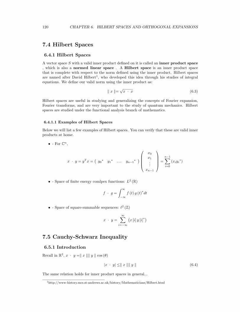
120 CHAPTER 6. HILBERT SPACES AND ORTHOGONAL EXPANSIONS
7.4 Hilbert Spaces
6.4.1 Hilbert Spaces
A vector space S with a valid inner product defined on it is called an inner product space, which is also a normed linear space . A Hilbert space is an inner product spacethat is complete with respect to the norm defined using the inner product. Hilbert spacesare named after David Hilbert1, who developed this idea through his studies of integralequations. We define our valid norm using the inner product as:
‖ x ‖=√x · x (6.3)
Hilbert spaces are useful in studying and generalizing the concepts of Fourier expansion,Fourier transforms, and are very important to the study of quantum mechanics. Hilbertspaces are studied under the functional analysis branch of mathematics.
6.4.1.1 Examples of Hilbert Spaces
Below we will list a few examples of Hilbert spaces. You can verify that these are valid innerproducts at home.
• - For Cn,
x · y = yTx =(y0∗ y1
∗ . . . yn−1∗ )
x0
x1
...xn−1
=n−1∑i=0
(xiyi∗)
• - Space of finite energy comlpex functions: L2 (R)
f · g =∫ ∞
−∞f (t) g (t)∗dt
• - Space of square-summable sequences: `2 (Z)
x · y =∞∑
i=−∞
(x [i] y [i]∗
)
7.5 Cauchy-Schwarz Inequality
6.5.1 Introduction
Recall in R2, x · y =‖ x ‖‖ y ‖ cos (θ)
|x · y| ≤‖ x ‖‖ y ‖ (6.4)
The same relation holds for inner product spaces in general...
1http://www-history.mcs.st-andrews.ac.uk/history/Mathematicians/Hilbert.html
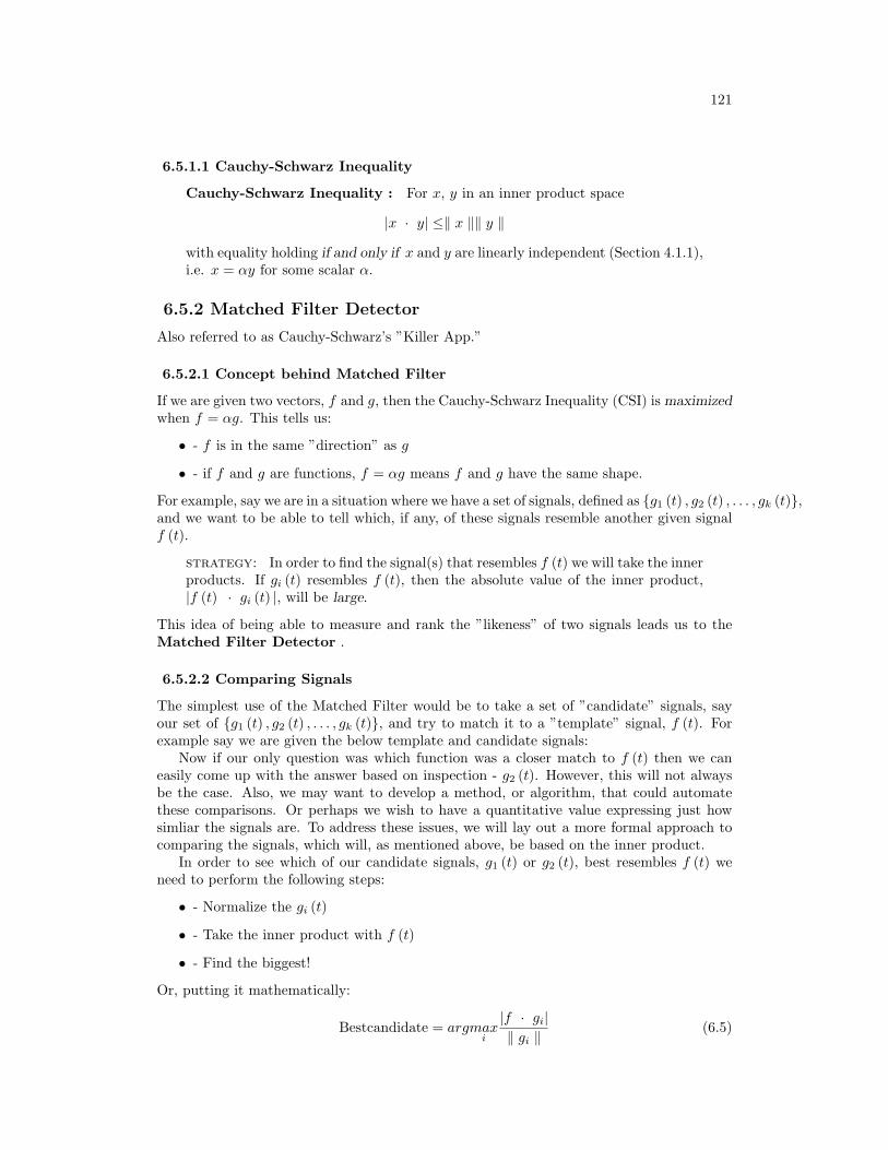
121
6.5.1.1 Cauchy-Schwarz Inequality
Cauchy-Schwarz Inequality : For x, y in an inner product space
|x · y| ≤‖ x ‖‖ y ‖
with equality holding if and only if x and y are linearly independent (Section 4.1.1),i.e. x = αy for some scalar α.
6.5.2 Matched Filter Detector
Also referred to as Cauchy-Schwarz’s ”Killer App.”
6.5.2.1 Concept behind Matched Filter
If we are given two vectors, f and g, then the Cauchy-Schwarz Inequality (CSI) is maximizedwhen f = αg. This tells us:
• - f is in the same ”direction” as g
• - if f and g are functions, f = αg means f and g have the same shape.
For example, say we are in a situation where we have a set of signals, defined as g1 (t) , g2 (t) , . . . , gk (t),and we want to be able to tell which, if any, of these signals resemble another given signalf (t).
strategy: In order to find the signal(s) that resembles f (t) we will take the innerproducts. If gi (t) resembles f (t), then the absolute value of the inner product,|f (t) · gi (t) |, will be large.
This idea of being able to measure and rank the ”likeness” of two signals leads us to theMatched Filter Detector .
6.5.2.2 Comparing Signals
The simplest use of the Matched Filter would be to take a set of ”candidate” signals, sayour set of g1 (t) , g2 (t) , . . . , gk (t), and try to match it to a ”template” signal, f (t). Forexample say we are given the below template and candidate signals:
Now if our only question was which function was a closer match to f (t) then we caneasily come up with the answer based on inspection - g2 (t). However, this will not alwaysbe the case. Also, we may want to develop a method, or algorithm, that could automatethese comparisons. Or perhaps we wish to have a quantitative value expressing just howsimliar the signals are. To address these issues, we will lay out a more formal approach tocomparing the signals, which will, as mentioned above, be based on the inner product.
In order to see which of our candidate signals, g1 (t) or g2 (t), best resembles f (t) weneed to perform the following steps:
• - Normalize the gi (t)
• - Take the inner product with f (t)
• - Find the biggest!
Or, putting it mathematically:
Bestcandidate = argmaxi
|f · gi|‖ gi ‖
(6.5)
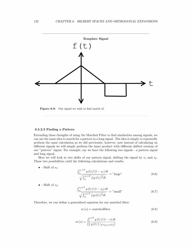
122 CHAPTER 6. HILBERT SPACES AND ORTHOGONAL EXPANSIONS
Template Signal
f(t)
t
Figure 6.8: Our signal we wish to find match of.
6.5.2.3 Finding a Pattern
Extending these thoughts of using the Matched Filter to find similarities among signals, wecan use the same idea to search for a pattern in a long signal. The idea is simply to repeatedlyperform the same calculation as we did previously; however, now instead of calculating ondifferent signals we will simply perform the inner product with different shifted versions ofour ”pattern” signal. For example, say we have the following two signals - a pattern signaland long signal.
Here we will look at two shifts of our pattern signal, shifting the signal by s1 and s2.These two possibilities yield the following calculations and results:
• - Shift of s1: ∫ s1+T
s1g (t) f (t− s1) dt√∫ s1+T
s1(|g (t) |)2dt
= ”large” (6.6)
• - Shift of s2: ∫ s2+T
s2g (t) f (t− s2) dt√∫ s2+T
s2(|g (t) |)2dt
= ”small” (6.7)
Therefore, we can define a generalized equation for our matched filter:
m (s) = matchedfilter (6.8)
m (s) =
∫ s+T
sg (t) f (t− s) dt(
‖ g (t) ‖ |L2([s,s+T ])
) (6.9)
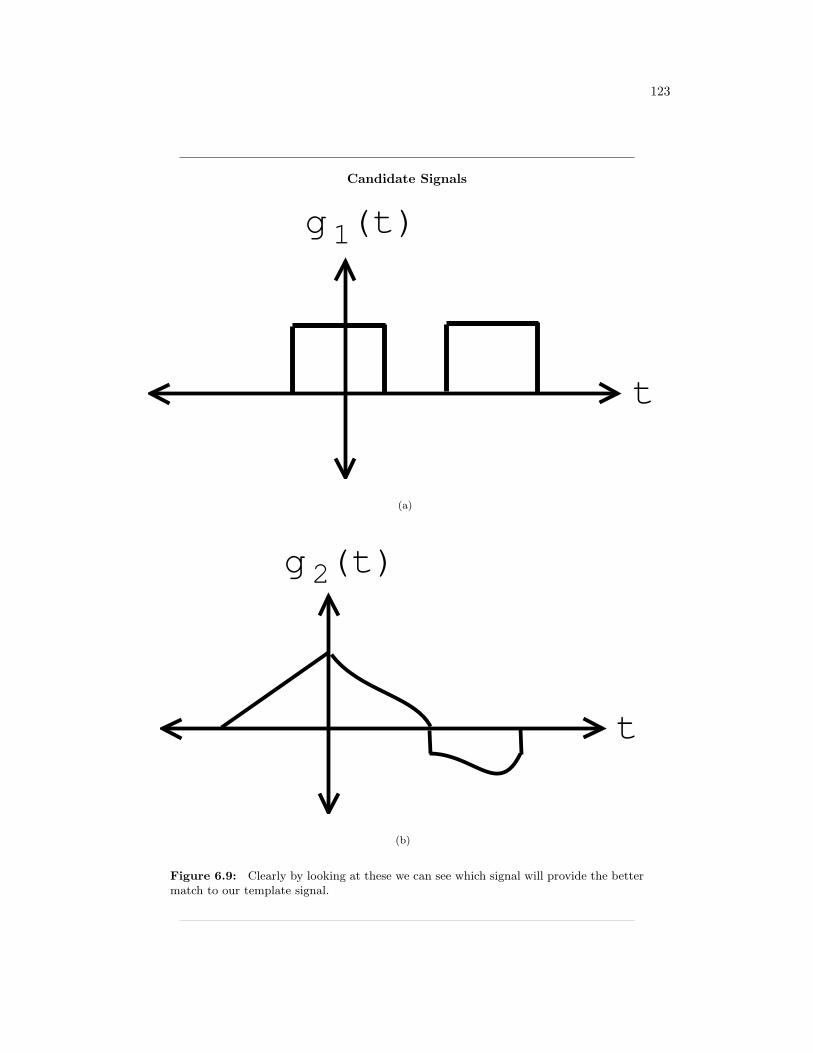
123
Candidate Signals
g (t)
t
1
(a)
g (t)
t
2
(b)
Figure 6.9: Clearly by looking at these we can see which signal will provide the bettermatch to our template signal.
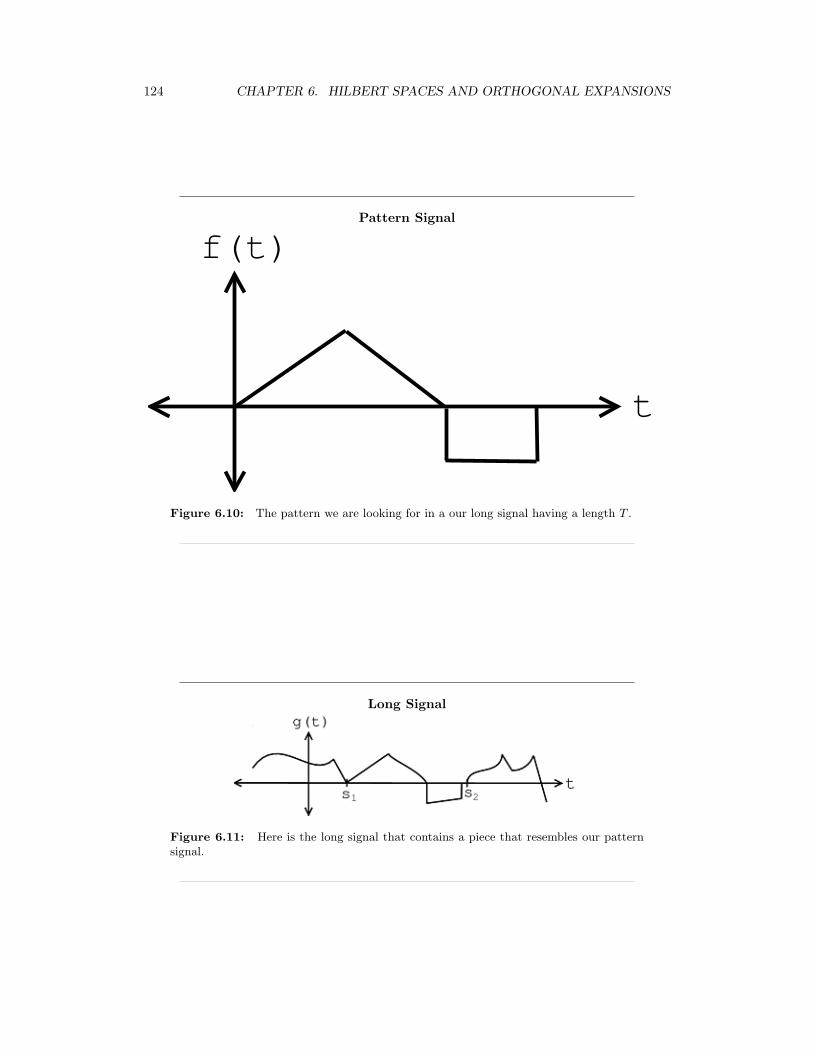
124 CHAPTER 6. HILBERT SPACES AND ORTHOGONAL EXPANSIONS
Pattern Signal
f(t)
t
Figure 6.10: The pattern we are looking for in a our long signal having a length T .
Long Signal
Figure 6.11: Here is the long signal that contains a piece that resembles our patternsignal.
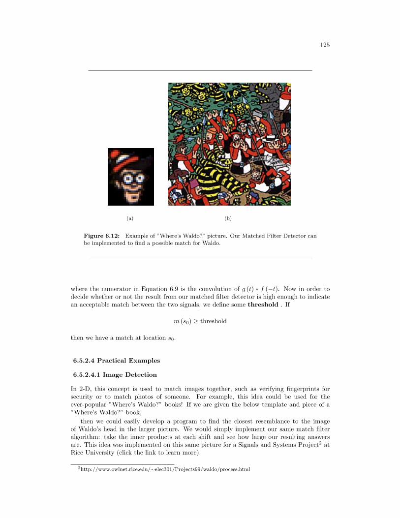
125
(a) (b)
Figure 6.12: Example of ”Where’s Waldo?” picture. Our Matched Filter Detector canbe implemented to find a possible match for Waldo.
where the numerator in Equation 6.9 is the convolution of g (t) ∗ f (−t). Now in order todecide whether or not the result from our matched filter detector is high enough to indicatean acceptable match between the two signals, we define some threshold . If
m (s0) ≥ threshold
then we have a match at location s0.
6.5.2.4 Practical Examples
6.5.2.4.1 Image Detection
In 2-D, this concept is used to match images together, such as verifying fingerprints forsecurity or to match photos of someone. For example, this idea could be used for theever-popular ”Where’s Waldo?” books! If we are given the below template and piece of a”Where’s Waldo?” book,
then we could easily develop a program to find the closest resemblance to the imageof Waldo’s head in the larger picture. We would simply implement our same match filteralgorithm: take the inner products at each shift and see how large our resulting answersare. This idea was implemented on this same picture for a Signals and Systems Project2 atRice University (click the link to learn more).
2http://www.owlnet.rice.edu/∼elec301/Projects99/waldo/process.html
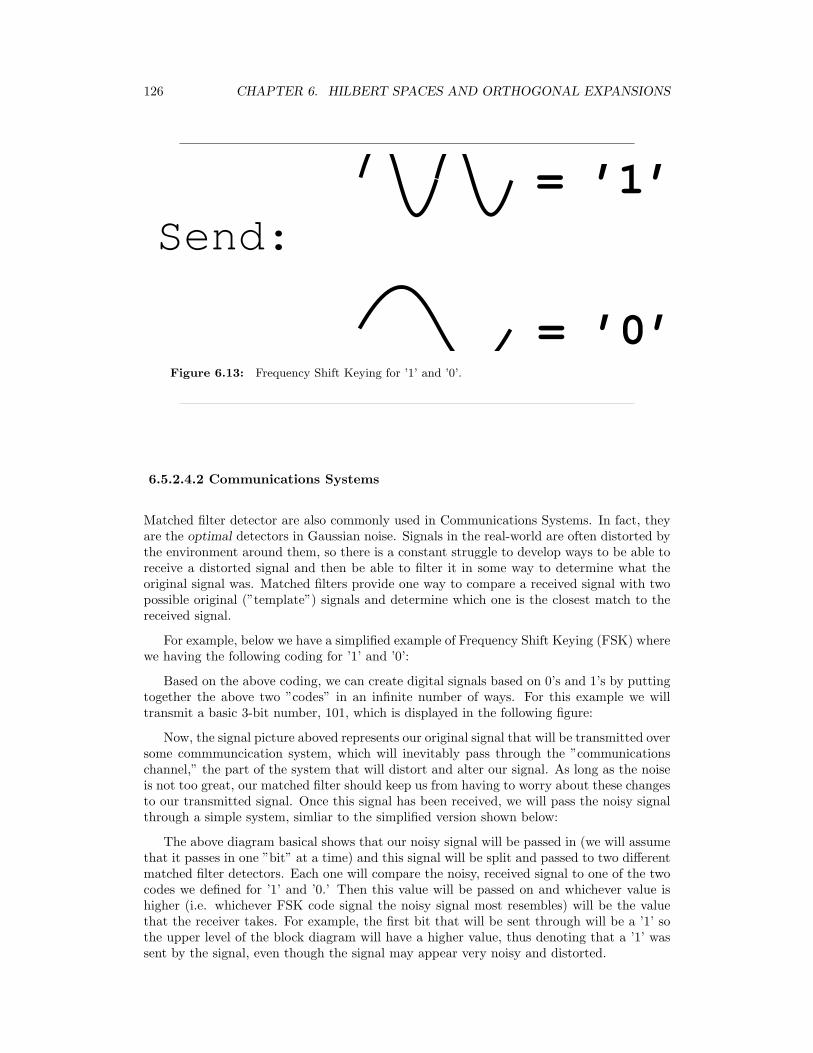
126 CHAPTER 6. HILBERT SPACES AND ORTHOGONAL EXPANSIONS
Send:= ’1’
= ’0’Figure 6.13: Frequency Shift Keying for ’1’ and ’0’.
6.5.2.4.2 Communications Systems
Matched filter detector are also commonly used in Communications Systems. In fact, theyare the optimal detectors in Gaussian noise. Signals in the real-world are often distorted bythe environment around them, so there is a constant struggle to develop ways to be able toreceive a distorted signal and then be able to filter it in some way to determine what theoriginal signal was. Matched filters provide one way to compare a received signal with twopossible original (”template”) signals and determine which one is the closest match to thereceived signal.
For example, below we have a simplified example of Frequency Shift Keying (FSK) wherewe having the following coding for ’1’ and ’0’:
Based on the above coding, we can create digital signals based on 0’s and 1’s by puttingtogether the above two ”codes” in an infinite number of ways. For this example we willtransmit a basic 3-bit number, 101, which is displayed in the following figure:
Now, the signal picture aboved represents our original signal that will be transmitted oversome commmuncication system, which will inevitably pass through the ”communicationschannel,” the part of the system that will distort and alter our signal. As long as the noiseis not too great, our matched filter should keep us from having to worry about these changesto our transmitted signal. Once this signal has been received, we will pass the noisy signalthrough a simple system, simliar to the simplified version shown below:
The above diagram basical shows that our noisy signal will be passed in (we will assumethat it passes in one ”bit” at a time) and this signal will be split and passed to two differentmatched filter detectors. Each one will compare the noisy, received signal to one of the twocodes we defined for ’1’ and ’0.’ Then this value will be passed on and whichever value ishigher (i.e. whichever FSK code signal the noisy signal most resembles) will be the valuethat the receiver takes. For example, the first bit that will be sent through will be a ’1’ sothe upper level of the block diagram will have a higher value, thus denoting that a ’1’ wassent by the signal, even though the signal may appear very noisy and distorted.
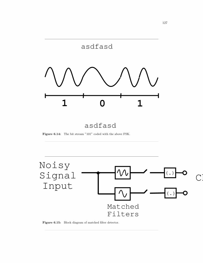
127
1 10
asdfasd
asdfasdFigure 6.14: The bit stream ”101” coded with the above FSK.
Noisy SignalInput
ChooseMax
(.)
(.)
MatchedFilters
Figure 6.15: Block diagram of matched filter detector.
128 CHAPTER 6. HILBERT SPACES AND ORTHOGONAL EXPANSIONS
6.5.3 Proof of CSI
Here will look at the proof of our Cauchy-Schwarz Inequality (CSI) for a real vector space.
Theorem 6.1: CSI for Real Vector Space
For f ∈ HilbertSpaceS and g ∈ HilbertSpaceS, show:
|f · g| ≤‖ f ‖‖ g ‖ (6.10)
with equality if and only if g = αf .
Proof:
•- If g = αf , show |f · g| =‖ f ‖‖ g ‖
|f · g| = |f · αf | = |α||f · f | = |α|(‖ f ‖)2
|f · g| =‖ f ‖ (|α| ‖ f ‖) =‖ f ‖‖ g ‖This verifies our above statement of the CSI!•- If g 6= αf , show |f · g| <‖ f ‖‖ g ‖ where we have ∀β, β ∈ R : βf + g 6= 0
0 < (‖ βf + g ‖)2 = βf + g · βf + g = β2f · f + 2βf · g + g · g
= β2(‖ f ‖)2 + 2βf · g + (‖ g ‖)2
And we get a quadritic in β. Visually, the quadratic polynomial in β > 0 forallβ. Also, note that this polynomial has no real roots and the discriminant isless than 0. - BLAH BLAH BLAH –
aβ2 + bβ + c
has discriminant β2 − 4ac where we have:
a = (‖ f ‖)2
b = 2f · gc = (‖ g ‖)2
Therefore, we can plug this values into the above polynomials discriminant toget:
4(|f · g|)2 − 4(‖ f ‖)2(‖ g ‖)2 < 0 (6.11)
|f · g| <‖ f ‖‖ g ‖ (6.12)
And finally we have proven the Cauchy-Schwarz Inequality formula for realvectors spaces.
question: What changes do we have to make to the proof for acomplex vector space? (try to figure this out at home)
7.6 Common Hilbert Spaces
6.6.1 Common Hilbert Spaces
Below we will look at the four most common Hilbert spaces that you will have to deal withwhen discussing and manipulating signals and systems.
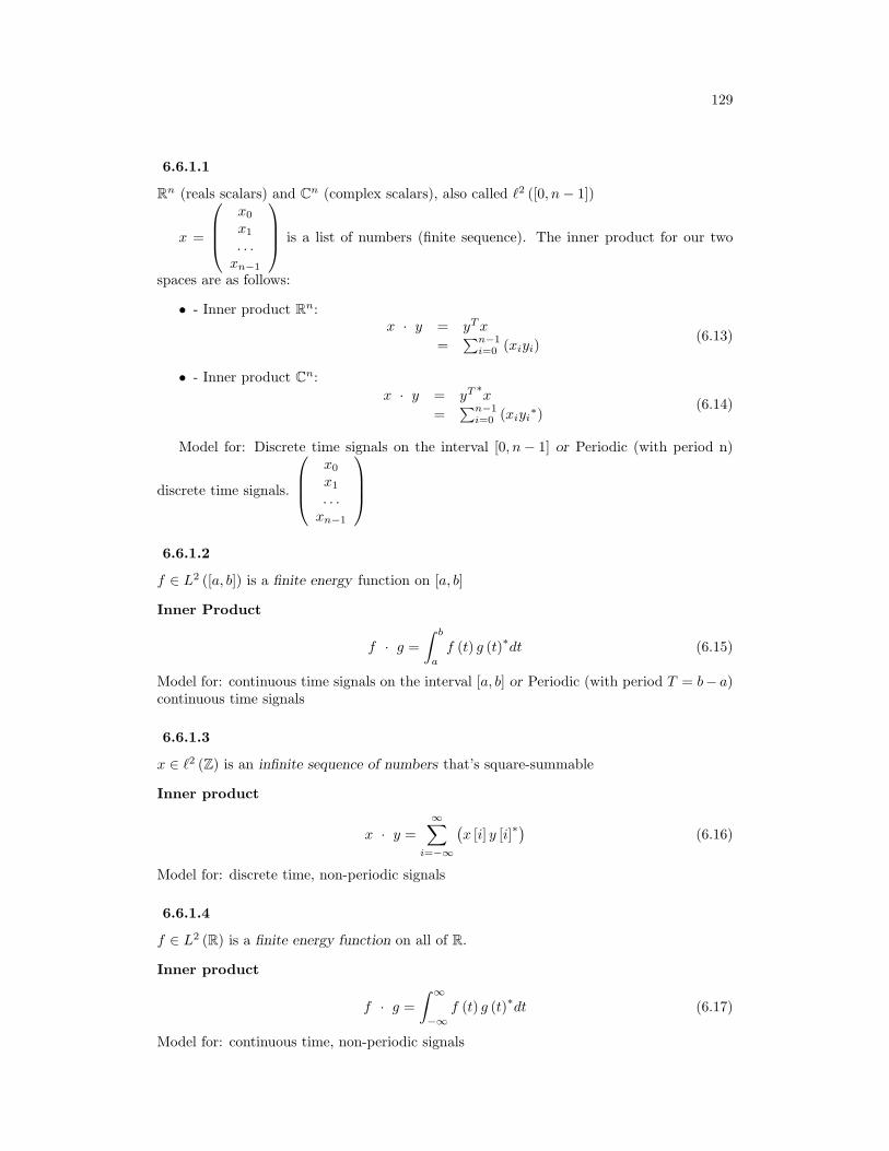
129
6.6.1.1
Rn (reals scalars) and Cn (complex scalars), also called `2 ([0, n− 1])
x =
x0
x1
. . .xn−1
is a list of numbers (finite sequence). The inner product for our two
spaces are as follows:
• - Inner product Rn:x · y = yTx
=∑n−1
i=0 (xiyi)(6.13)
• - Inner product Cn:x · y = yT ∗x
=∑n−1
i=0 (xiyi∗)
(6.14)
Model for: Discrete time signals on the interval [0, n− 1] or Periodic (with period n)
discrete time signals.
x0
x1
. . .xn−1
6.6.1.2
f ∈ L2 ([a, b]) is a finite energy function on [a, b]
Inner Product
f · g =∫ b
a
f (t) g (t)∗dt (6.15)
Model for: continuous time signals on the interval [a, b] or Periodic (with period T = b− a)continuous time signals
6.6.1.3
x ∈ `2 (Z) is an infinite sequence of numbers that’s square-summable
Inner product
x · y =∞∑
i=−∞
(x [i] y [i]∗
)(6.16)
Model for: discrete time, non-periodic signals
6.6.1.4
f ∈ L2 (R) is a finite energy function on all of R.
Inner product
f · g =∫ ∞
−∞f (t) g (t)∗dt (6.17)
Model for: continuous time, non-periodic signals
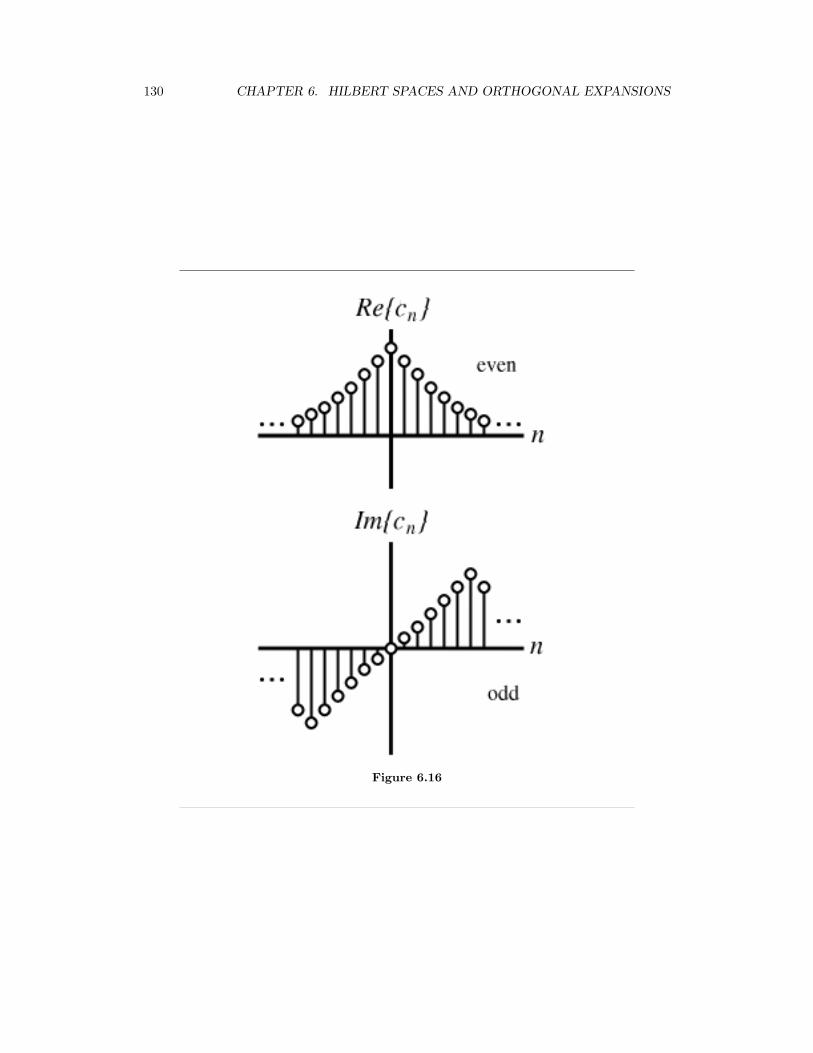
130 CHAPTER 6. HILBERT SPACES AND ORTHOGONAL EXPANSIONS
Figure 6.16
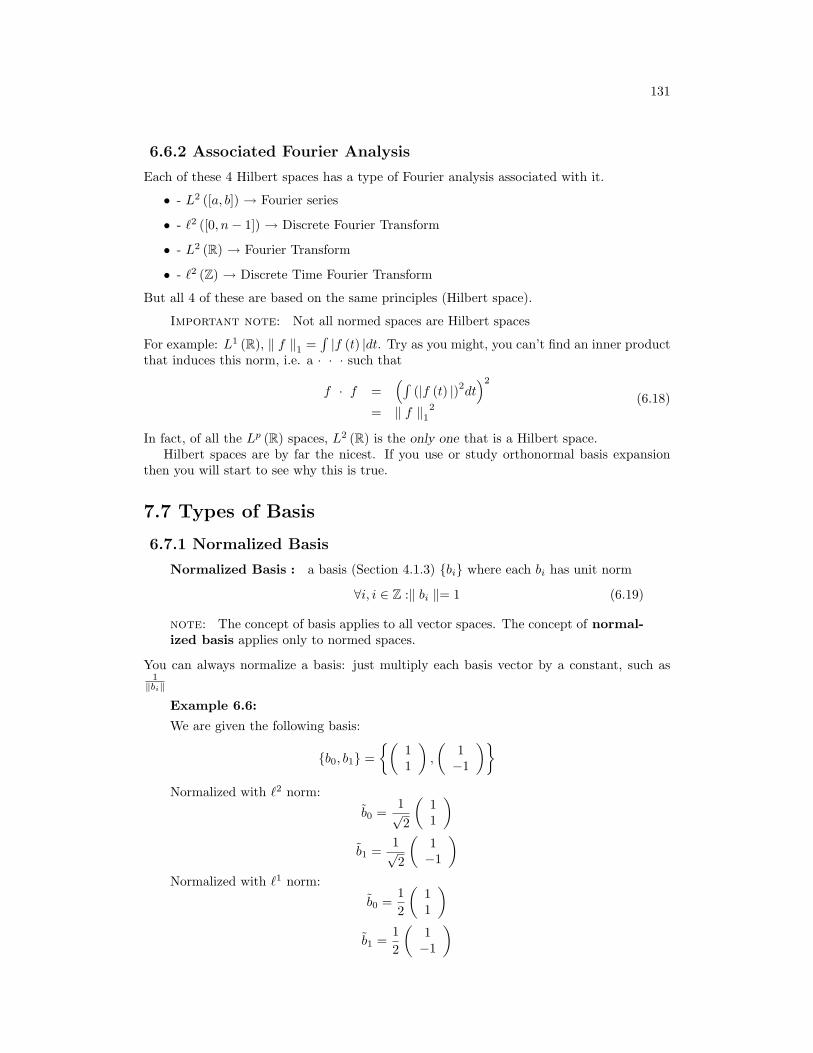
131
6.6.2 Associated Fourier Analysis
Each of these 4 Hilbert spaces has a type of Fourier analysis associated with it.
• - L2 ([a, b]) → Fourier series
• - `2 ([0, n− 1]) → Discrete Fourier Transform
• - L2 (R) → Fourier Transform
• - `2 (Z) → Discrete Time Fourier Transform
But all 4 of these are based on the same principles (Hilbert space).
Important note: Not all normed spaces are Hilbert spaces
For example: L1 (R), ‖ f ‖1 =∫|f (t) |dt. Try as you might, you can’t find an inner product
that induces this norm, i.e. a · · · such that
f · f =(∫
(|f (t) |)2dt)2
= ‖ f ‖12
(6.18)
In fact, of all the Lp (R) spaces, L2 (R) is the only one that is a Hilbert space.Hilbert spaces are by far the nicest. If you use or study orthonormal basis expansion
then you will start to see why this is true.
7.7 Types of Basis
6.7.1 Normalized Basis
Normalized Basis : a basis (Section 4.1.3) bi where each bi has unit norm
∀i, i ∈ Z :‖ bi ‖= 1 (6.19)
note: The concept of basis applies to all vector spaces. The concept of normal-ized basis applies only to normed spaces.
You can always normalize a basis: just multiply each basis vector by a constant, such as1
‖bi‖
Example 6.6:
We are given the following basis:
b0, b1 =(
11
),
(1−1
)Normalized with `2 norm:
b0 =1√2
(11
)b1 =
1√2
(1−1
)Normalized with `1 norm:
b0 =12
(11
)b1 =
12
(1−1
)
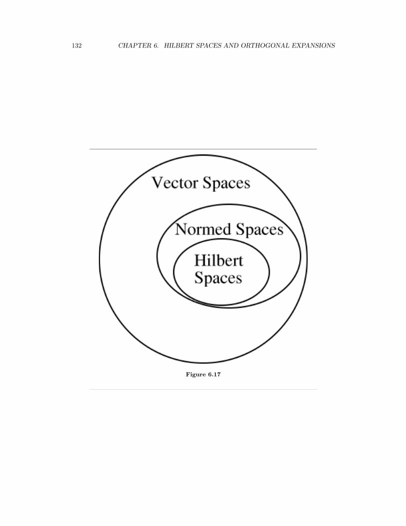
132 CHAPTER 6. HILBERT SPACES AND ORTHOGONAL EXPANSIONS
Figure 6.17
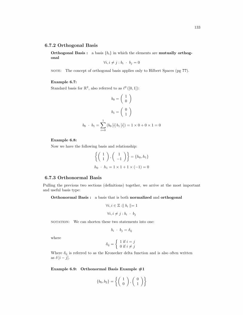
133
6.7.2 Orthogonal Basis
Orthogonal Basis : a basis bi in which the elements are mutually orthog-onal
∀i, i 6= j : bi · bj = 0
note: The concept of orthogonal basis applies only to Hilbert Spaces (pg ??).
Example 6.7:
Standard basis for R2, also referred to as `2 ([0, 1]):
b0 =(
10
)
b1 =(
01
)
b0 · b1 =1∑
i=0
(b0 [i] b1 [i]) = 1× 0 + 0× 1 = 0
Example 6.8:
Now we have the following basis and relationship:(11
),
(1−1
)= h0, h1
h0 · h1 = 1× 1 + 1× (−1) = 0
6.7.3 Orthonormal Basis
Pulling the previous two sections (definitions) together, we arrive at the most importantand useful basis type:
Orthonormal Basis : a basis that is both normalized and orthogonal
∀i, i ∈ Z :‖ bi ‖= 1
∀i, i 6= j : bi · bj
notation: We can shorten these two statements into one:
bi · bj = δij
where
δij =
1 if i = j0 if i 6= j
Where δij is referred to as the Kronecker delta function and is also often writtenas δ [i− j].
Example 6.9: Orthonormal Basis Example #1
b0, b2 =(
10
),
(01
)
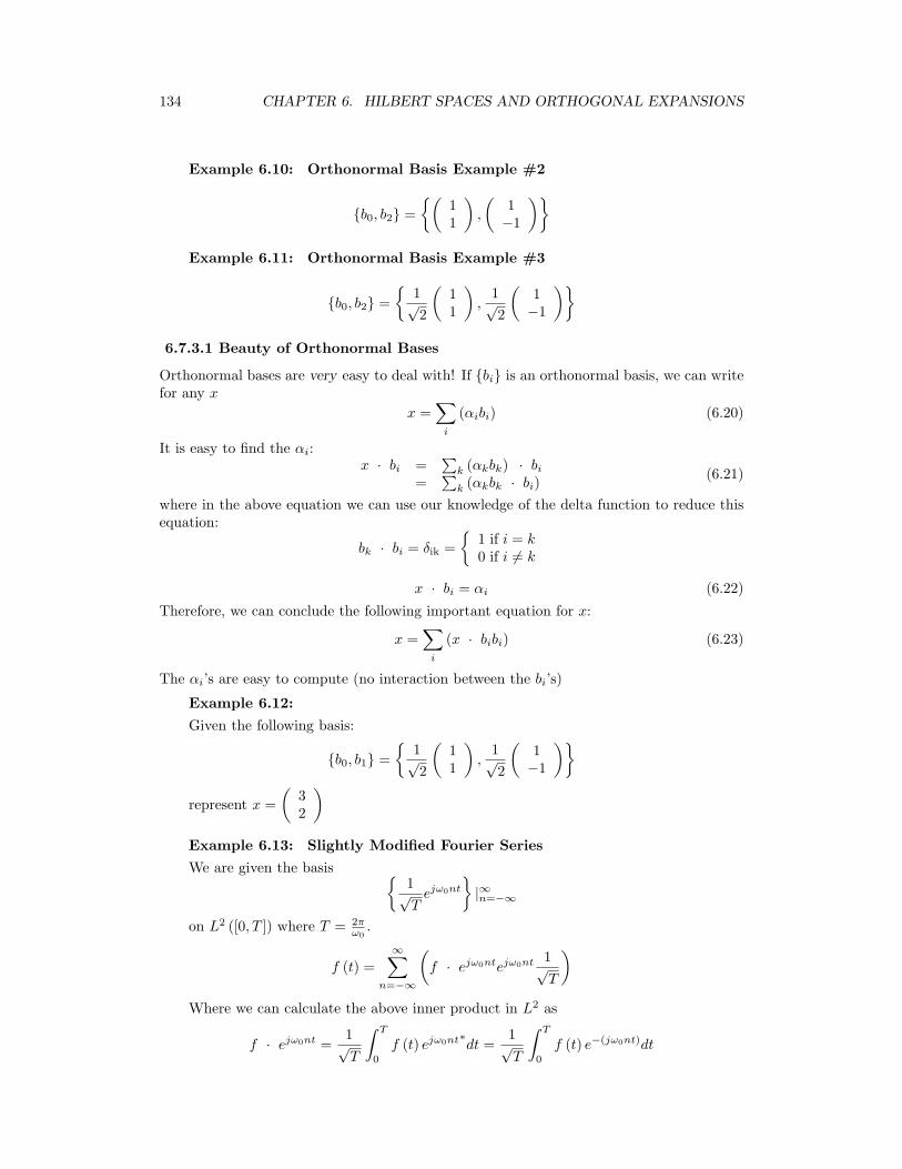
134 CHAPTER 6. HILBERT SPACES AND ORTHOGONAL EXPANSIONS
Example 6.10: Orthonormal Basis Example #2
b0, b2 =(
11
),
(1−1
)Example 6.11: Orthonormal Basis Example #3
b0, b2 =
1√2
(11
),
1√2
(1−1
)6.7.3.1 Beauty of Orthonormal Bases
Orthonormal bases are very easy to deal with! If bi is an orthonormal basis, we can writefor any x
x =∑
i
(αibi) (6.20)
It is easy to find the αi:x · bi =
∑k (αkbk) · bi
=∑
k (αkbk · bi)(6.21)
where in the above equation we can use our knowledge of the delta function to reduce thisequation:
bk · bi = δik =
1 if i = k0 if i 6= k
x · bi = αi (6.22)
Therefore, we can conclude the following important equation for x:
x =∑
i
(x · bibi) (6.23)
The αi’s are easy to compute (no interaction between the bi’s)
Example 6.12:
Given the following basis:
b0, b1 =
1√2
(11
),
1√2
(1−1
)represent x =
(32
)Example 6.13: Slightly Modified Fourier Series
We are given the basis 1√Tejω0nt
|∞n=−∞
on L2 ([0, T ]) where T = 2πω0
.
f (t) =∞∑
n=−∞
(f · ejω0ntejω0nt 1√
T
)Where we can calculate the above inner product in L2 as
f · ejω0nt =1√T
∫ T
0
f (t) ejω0nt∗dt =1√T
∫ T
0
f (t) e−(jω0nt)dt
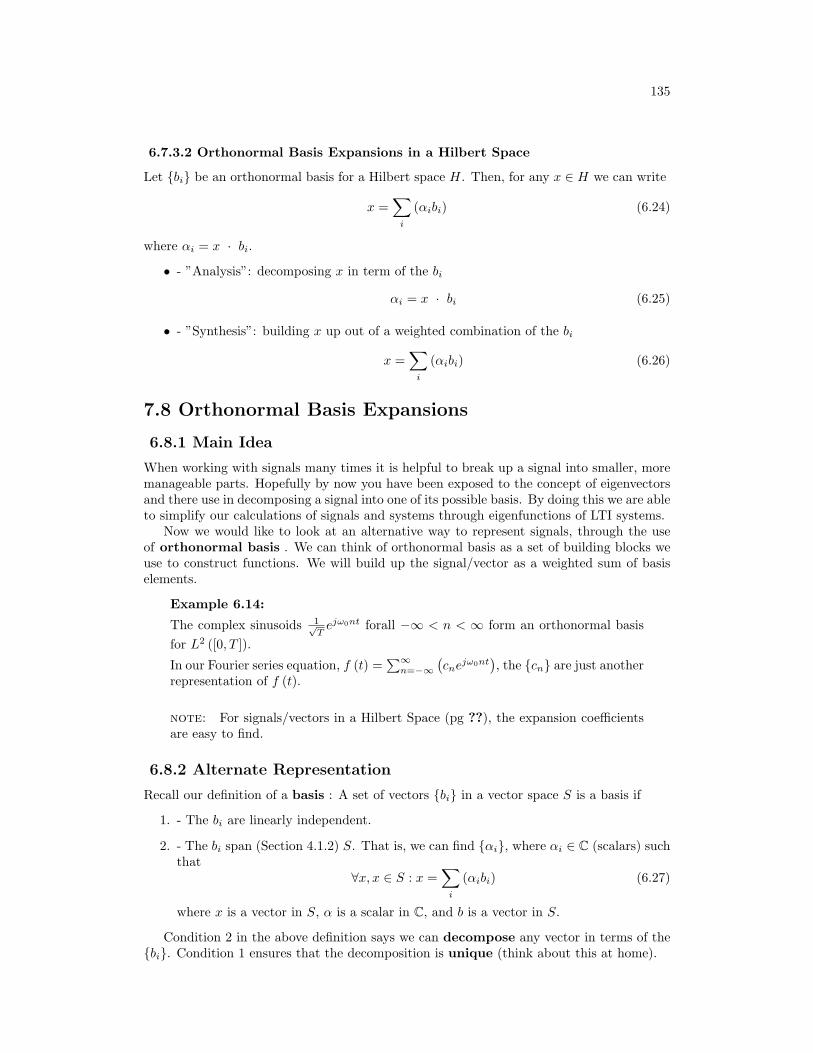
135
6.7.3.2 Orthonormal Basis Expansions in a Hilbert Space
Let bi be an orthonormal basis for a Hilbert space H. Then, for any x ∈ H we can write
x =∑
i
(αibi) (6.24)
where αi = x · bi.
• - ”Analysis”: decomposing x in term of the bi
αi = x · bi (6.25)
• - ”Synthesis”: building x up out of a weighted combination of the bi
x =∑
i
(αibi) (6.26)
7.8 Orthonormal Basis Expansions
6.8.1 Main Idea
When working with signals many times it is helpful to break up a signal into smaller, moremanageable parts. Hopefully by now you have been exposed to the concept of eigenvectorsand there use in decomposing a signal into one of its possible basis. By doing this we are ableto simplify our calculations of signals and systems through eigenfunctions of LTI systems.
Now we would like to look at an alternative way to represent signals, through the useof orthonormal basis . We can think of orthonormal basis as a set of building blocks weuse to construct functions. We will build up the signal/vector as a weighted sum of basiselements.
Example 6.14:
The complex sinusoids 1√Tejω0nt forall −∞ < n < ∞ form an orthonormal basis
for L2 ([0, T ]).
In our Fourier series equation, f (t) =∑∞
n=−∞(cne
jω0nt), the cn are just another
representation of f (t).
note: For signals/vectors in a Hilbert Space (pg ??), the expansion coefficientsare easy to find.
6.8.2 Alternate Representation
Recall our definition of a basis : A set of vectors bi in a vector space S is a basis if
1. - The bi are linearly independent.
2. - The bi span (Section 4.1.2) S. That is, we can find αi, where αi ∈ C (scalars) suchthat
∀x, x ∈ S : x =∑
i
(αibi) (6.27)
where x is a vector in S, α is a scalar in C, and b is a vector in S.
Condition 2 in the above definition says we can decompose any vector in terms of thebi. Condition 1 ensures that the decomposition is unique (think about this at home).
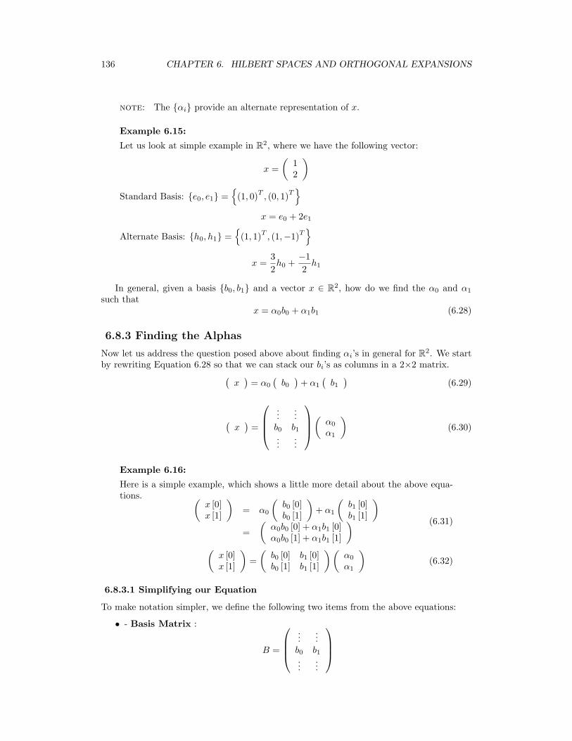
136 CHAPTER 6. HILBERT SPACES AND ORTHOGONAL EXPANSIONS
note: The αi provide an alternate representation of x.
Example 6.15:
Let us look at simple example in R2, where we have the following vector:
x =(
12
)Standard Basis: e0, e1 =
(1, 0)T
, (0, 1)T
x = e0 + 2e1
Alternate Basis: h0, h1 =
(1, 1)T, (1,−1)T
x =
32h0 +
−12h1
In general, given a basis b0, b1 and a vector x ∈ R2, how do we find the α0 and α1
such thatx = α0b0 + α1b1 (6.28)
6.8.3 Finding the Alphas
Now let us address the question posed above about finding αi’s in general for R2. We startby rewriting Equation 6.28 so that we can stack our bi’s as columns in a 2×2 matrix.(
x)
= α0
(b0)
+ α1
(b1)
(6.29)
(x)
=
...
...b0 b1...
...
( α0
α1
)(6.30)
Example 6.16:
Here is a simple example, which shows a little more detail about the above equa-tions. (
x [0]x [1]
)= α0
(b0 [0]b0 [1]
)+ α1
(b1 [0]b1 [1]
)=
(α0b0 [0] + α1b1 [0]α0b0 [1] + α1b1 [1]
) (6.31)
(x [0]x [1]
)=(b0 [0] b1 [0]b0 [1] b1 [1]
)(α0
α1
)(6.32)
6.8.3.1 Simplifying our Equation
To make notation simpler, we define the following two items from the above equations:
• - Basis Matrix :
B =
...
...b0 b1...
...
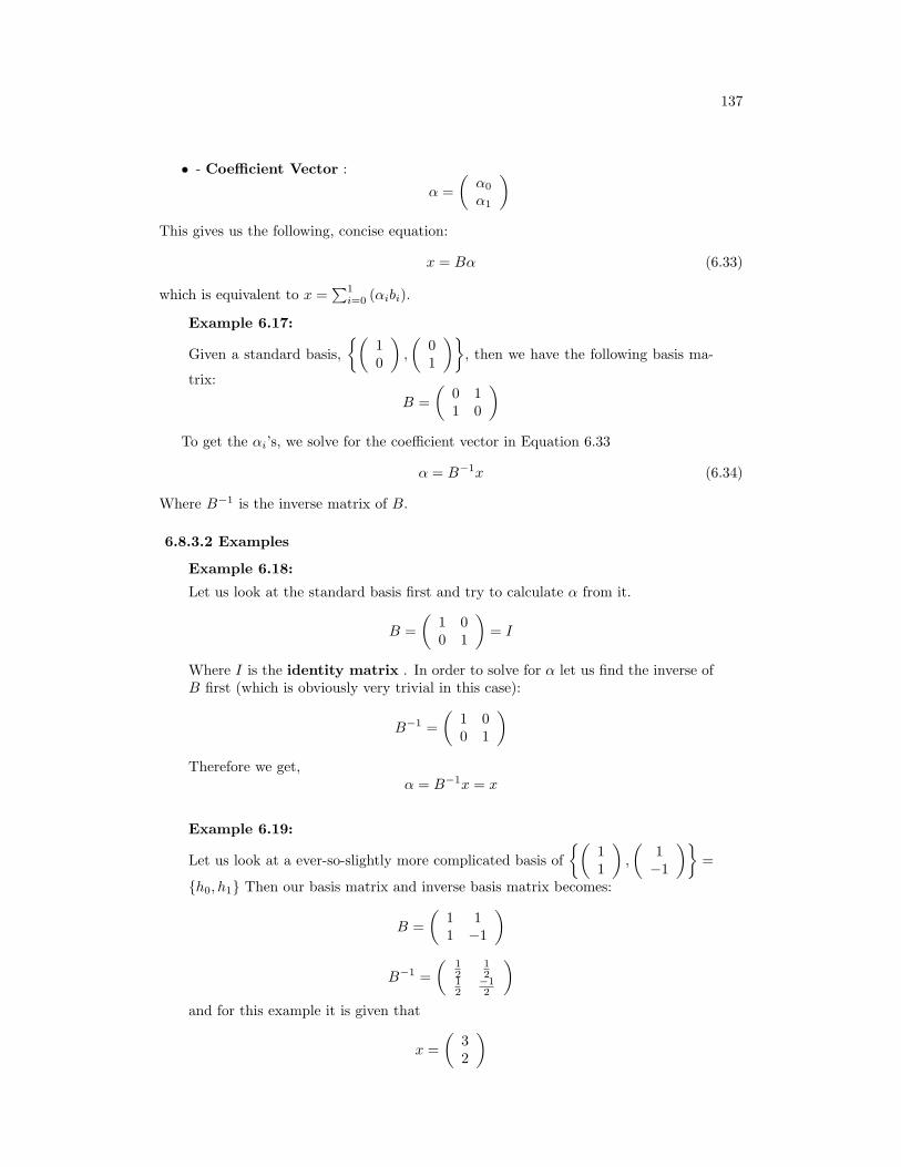
137
• - Coefficient Vector :
α =(α0
α1
)This gives us the following, concise equation:
x = Bα (6.33)
which is equivalent to x =∑1
i=0 (αibi).
Example 6.17:
Given a standard basis,(
10
),
(01
), then we have the following basis ma-
trix:
B =(
0 11 0
)To get the αi’s, we solve for the coefficient vector in Equation 6.33
α = B−1x (6.34)
Where B−1 is the inverse matrix of B.
6.8.3.2 Examples
Example 6.18:
Let us look at the standard basis first and try to calculate α from it.
B =(
1 00 1
)= I
Where I is the identity matrix . In order to solve for α let us find the inverse ofB first (which is obviously very trivial in this case):
B−1 =(
1 00 1
)Therefore we get,
α = B−1x = x
Example 6.19:
Let us look at a ever-so-slightly more complicated basis of(
11
),
(1−1
)=
h0, h1 Then our basis matrix and inverse basis matrix becomes:
B =(
1 11 −1
)
B−1 =(
12
12
12
−12
)and for this example it is given that
x =(
32
)
138 CHAPTER 6. HILBERT SPACES AND ORTHOGONAL EXPANSIONS
Now we solve for α
α = B−1x =(
12
12
12
−12
)(32
)=(
2.50.5
)and we get
x = 2.5h0 + 0.5h1
Exercise 6.1:
Now we are given the following basis matrix and x:
b0, b1 =(
12
),
(30
)
x =(
32
)For this problem, make a sketch of the bases and then represent x in terms of b0and b1.
Solution:In order to represent x in terms of b0 and b1 we will follow the same steps we usedin the above example.
B =(
1 23 0
)B−1 =
(0 1
213
−16
)α = B−1x =
(123
)And now we can write x in terms of b0 and b1.
x = b0 +23b1
And we can easily substitute in our known values of b0 and b1 to verify our results.
note: A change of basis simply looks at x from a ”different perspective.” B−1
transforms x from the standard basis to our new basis, b0, b1. Notice that thisis a totally mechanical procedure.
6.8.4 Extending the Dimension and Space
We can also extend all these ideas past just R2 and look at them in Rn and Cn. Thisprocedure extends naturally to higher (>2) dimensions. Given a basis b0, b1, . . . , bn−1 forRn, we want to find α0, α1, . . . , αn−1 such that
x = α0b0 + α1b1 + · · ·+ αn−1bn−1 (6.35)
Again, we will set up a basis matrix
B =(b0 b1 b2 . . . bn−1
)
139
where the columns equal the basis vectors and it will always be an n×n matrix (althoughthe above matrix does not appear to be square since we left terms in vector notation). Wecan then proceed to rewrite Equation 6.33
x =(b0 b1 . . . bn−1
) α0
...αn−1
= Bα
andα = B−1x
7.9 Function Space
We can also find basis vectors for vector spaces other than Rn.Let Pn be the vector space of n-th order polynomials on (-1, 1) with real coefficients
(verify P2 is a v.s. at home).
Example 6.20:
P2 = all quadratic polynomials. Let b0 (t) = 1, b1 (t) = t, b2 (t) = t2.
b0 (t) , b1 (t) , b2 (t) span P2, i.e. you can write any f (t) ∈ P2 as
f (t) = α0b0 (t) + α1b1 (t) + α2b2 (t)
for some αi ∈ R.
Note: P2 is 3 dimensional.
f (t) = t2 − 3t− 4
Alternate basis
b0 (t) , b1 (t) , b2 (t) =
1, t,12(3t2 − 1
)write f(t) in terms of this new basis d0 (t) = b0 (t), d1 (t) = b1 (t), d2 (t) = 3
2b2 (t)−12b0 (t).
f (t) = t2 − 3t− 4 = 4b0 (t)− 3b1 (t) + b2 (t)
f (t) = β0d0 (t) + β1d1 (t) + β2d2 (t) = β0b0 (t) + β1b1 (t) + β2
(32b2 (t)− 1
2b0 (t)
)f (t) =
(β0 −
12
)b0 (t) + β1b1 (t) +
32β2b2 (t)
soβ0 −
12
= 4
β1 = −3
32β2 = 1
then we get
f (t) = 4.5d0 (t)− 3d1 (t) +23d2 (t)
140 CHAPTER 6. HILBERT SPACES AND ORTHOGONAL EXPANSIONS
Example 6.21:
ejω0nt|∞n=−∞ is a basis for L2 ([0, T ]), T = 2πω0
, f (t) =∑
n
(Cne
jω0nt).
We calculate the expansion coefficients with
”change of basis” formula
Cn =1T
∫ T
0
f (t) e−(jω0nt)dt (6.36)
note: There are an infinite number of elments in the basis set, thatmeans L2 ([0, T ]) is infinite dimensional (scary!)
Infinite-dimensional spaces are hard to visualize. We can get a handle on theintuition by recognizing they share many of the same mathematical properties withfinite dimensional spaces. Many concepts apply to both (like ”basis expansion”).Some don’t (change of basis isn’t a nice matrix formula).
7.10 Haar Wavelet Basis
6.10.1 Introduction
Fourier series is a useful orthonormal representation on L2 ([0, T ]) especiallly for inputs intoLTI systems. However, it is ill suited for some applications, i.e. image processing (recallGibb’s phenomena).
Wavelets , discovered in the last 15 years, are another kind of basis for L2 ([0, T ]) andhave many nice properties.
6.10.2 Basis Comparisons
Fourier series - cn give frequency information. Basis functions last the entire interval.Wavelets - basis functions give frequency info but are local in time.In Fourier basis, the basis functions are harmonic multiples of ejω0t
In Haar wavelet basis, the basis functions are scaled and translated versions of a ”motherwavelet” ψ (t).
Basis functions ψj,k (t) are indexed by a scale j and a shift k.
Let ∀, 0 ≤ t < T : φ (t) = 1 Thenφ (t) , 2
j2ψ(2jt− k
)|j ∈ Z k = 0, 1, 2, . . . , 2j − 1
ψ (t) =
1 if 0 ≤ t < T
2
−1 if 0 ≤ T2 < T
(6.37)
Let ψj,k (t) = 2j2ψ(2jt− k
)Larger j → ”skinnier” basis function, j = 0, 1, 2, . . . , 2j shifts at each scale: k =
0, 1, . . . , 2j − 1Check: each ψj,k (t) has unit energy∫
ψj,k2 (t) dt = 1 ⇒ ‖ ψj,k (t) ‖2 = 1 (6.38)
Any two basis functions are orthogonal.Also, ψj,k, φ span L2 ([0, T ])
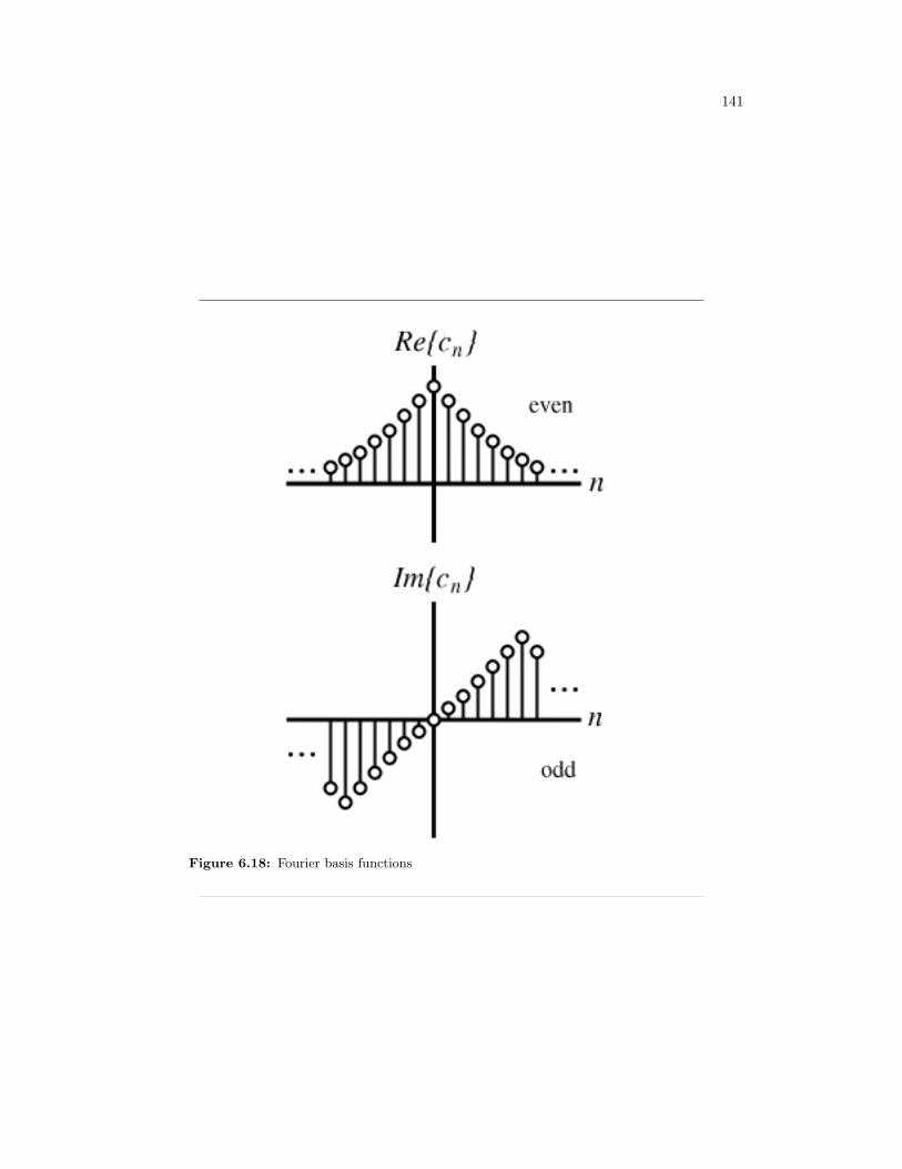
141
Figure 6.18: Fourier basis functions
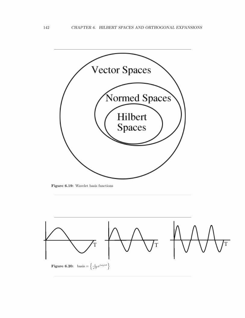
142 CHAPTER 6. HILBERT SPACES AND ORTHOGONAL EXPANSIONS
Figure 6.19: Wavelet basis functions
Figure 6.20: basis =
1√T
ejω0nt
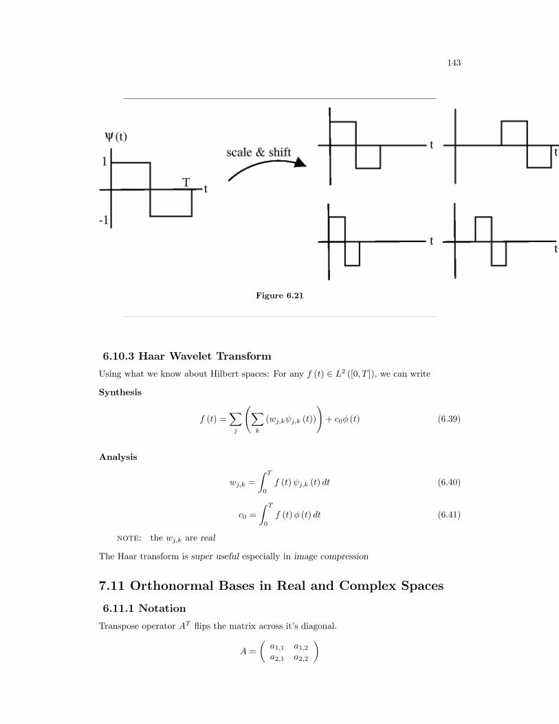
143
Figure 6.21
6.10.3 Haar Wavelet Transform
Using what we know about Hilbert spaces: For any f (t) ∈ L2 ([0, T ]), we can write
Synthesis
f (t) =∑
j
(∑k
(wj,kψj,k (t))
)+ c0φ (t) (6.39)
Analysis
wj,k =∫ T
0
f (t)ψj,k (t) dt (6.40)
c0 =∫ T
0
f (t)φ (t) dt (6.41)
note: the wj,k are real
The Haar transform is super useful especially in image compression
7.11 Orthonormal Bases in Real and Complex Spaces
6.11.1 Notation
Transpose operator AT flips the matrix across it’s diagonal.
A =(a1,1 a1,2
a2,1 a2,2
)
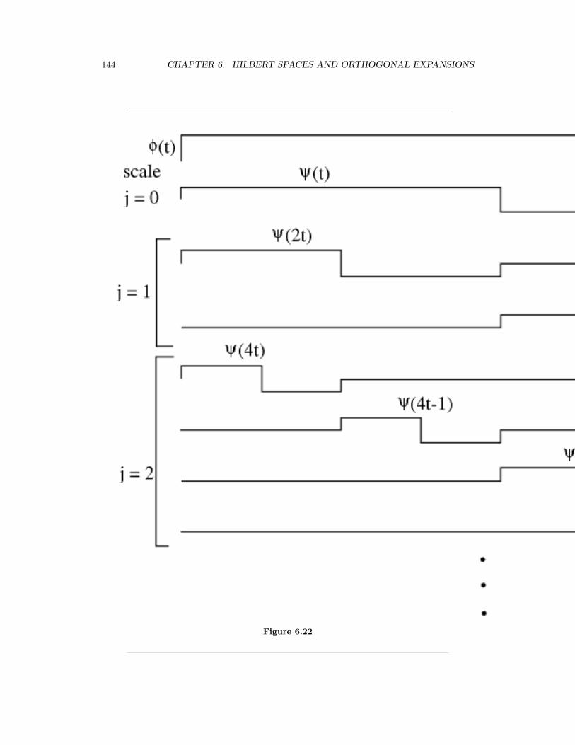
144 CHAPTER 6. HILBERT SPACES AND ORTHOGONAL EXPANSIONS
Figure 6.22
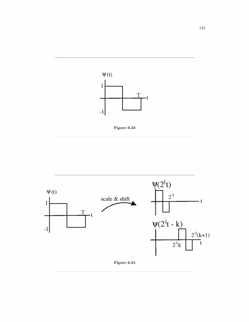
145
Figure 6.23
Figure 6.24
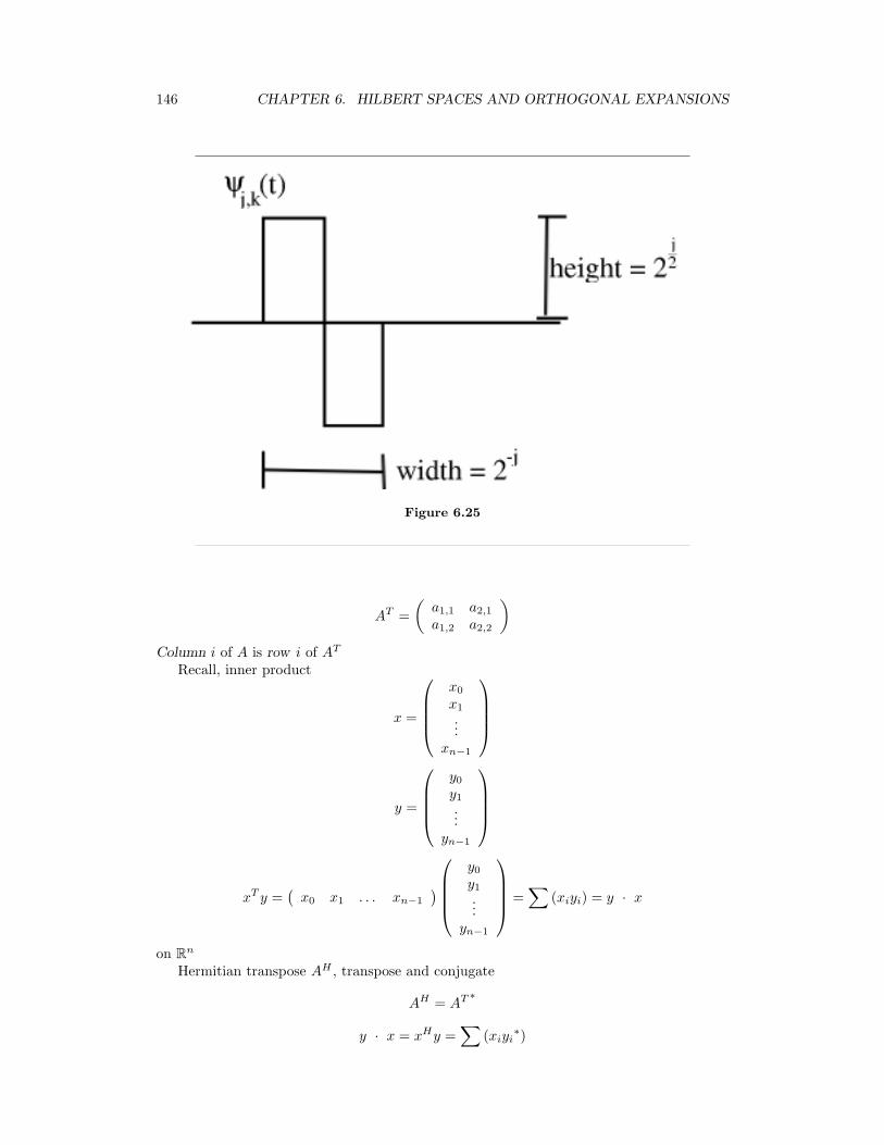
146 CHAPTER 6. HILBERT SPACES AND ORTHOGONAL EXPANSIONS
Figure 6.25
AT =(a1,1 a2,1
a1,2 a2,2
)Column i of A is row i of AT
Recall, inner product
x =
x0
x1
...xn−1
y =
y0y1...
yn−1
xT y =(x0 x1 . . . xn−1
)
y0y1...
yn−1
=∑
(xiyi) = y · x
on Rn
Hermitian transpose AH , transpose and conjugate
AH = AT ∗
y · x = xHy =∑
(xiyi∗)
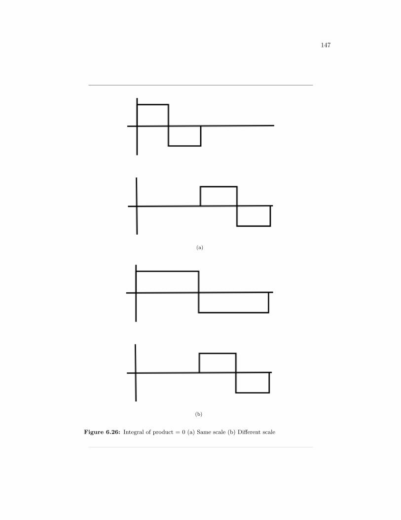
147
(a)
(b)
Figure 6.26: Integral of product = 0 (a) Same scale (b) Different scale
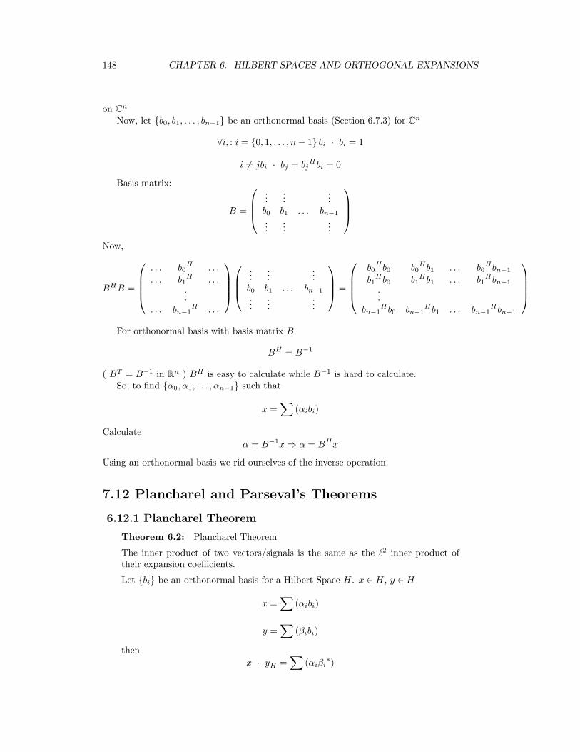
148 CHAPTER 6. HILBERT SPACES AND ORTHOGONAL EXPANSIONS
on Cn
Now, let b0, b1, . . . , bn−1 be an orthonormal basis (Section 6.7.3) for Cn
∀i, : i = 0, 1, . . . , n− 1 bi · bi = 1
i 6= jbi · bj = bjHbi = 0
Basis matrix:
B =
...
......
b0 b1 . . . bn−1
......
...
Now,
BHB =
. . . b0
H . . .
. . . b1H . . ....
. . . bn−1H . . .
......
...b0 b1 . . . bn−1
......
...
=
b0
Hb0 b0Hb1 . . . b0
Hbn−1
b1Hb0 b1
Hb1 . . . b1Hbn−1
...bn−1
Hb0 bn−1Hb1 . . . bn−1
Hbn−1
For orthonormal basis with basis matrix B
BH = B−1
( BT = B−1 in Rn ) BH is easy to calculate while B−1 is hard to calculate.So, to find α0, α1, . . . , αn−1 such that
x =∑
(αibi)
Calculateα = B−1x⇒ α = BHx
Using an orthonormal basis we rid ourselves of the inverse operation.
7.12 Plancharel and Parseval’s Theorems
6.12.1 Plancharel Theorem
Theorem 6.2: Plancharel Theorem
The inner product of two vectors/signals is the same as the `2 inner product oftheir expansion coefficients.
Let bi be an orthonormal basis for a Hilbert Space H. x ∈ H, y ∈ H
x =∑
(αibi)
y =∑
(βibi)
thenx · yH =
∑(αiβi
∗)
149
Example 6.22:Applying the Fourier Series, we gan go from f (t) to cn and g (t) todn ∫ T
0
f (t) g (t)∗dt =∞∑
n=−∞(cndn
∗)
inner product in time-domain = inner product of Fourier coefficients
Proof:
x =∑
(αibi)
y =∑
(βjbj)
x · yH =∑
(αibi) ·∑
(βjbj) =(∑
αi
)bi ·
∑(βjbj) =
(∑αi
)(∑(βj
∗))bi · bj =
∑(αiβi
∗)
by using inner product rules (pg 119)
note: bi · bj = 0 when i 6= j and bi · bj = 1 when i = j
If Hilbert space H has a ONB, then inner products are equivalent to inner productsin `2.All H with ONB are somehow equivalent to `2.
point of interest: square-summable sequences are important
6.12.2 Parseval’s Theorem
Theorem 6.3: Parseval’s Theorem
Energy of a signal = sum of squares of it’s expansion coefficients
Let x ∈ H, bi ONB
x =∑
(αibi)
Then(‖ x ‖H)2 =
∑((|αi|)2
)Proof:Directly from Plancharel
(‖ x ‖H)2 = x · xH =∑
(αiαi∗) =
∑((|αi|)2
)Example 6.23:Fourier Series 1√
Tejw0nt
f (t) =1√T
∑(cn
1√Tejw0nt
)∫ T
0
(|f (t) |)2dt =∞∑
n=−∞
((|cn|)2
)
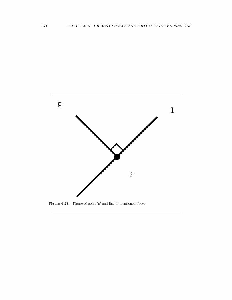
150 CHAPTER 6. HILBERT SPACES AND ORTHOGONAL EXPANSIONS
pl
p
Figure 6.27: Figure of point ’p’ and line ’l’ mentioned above.
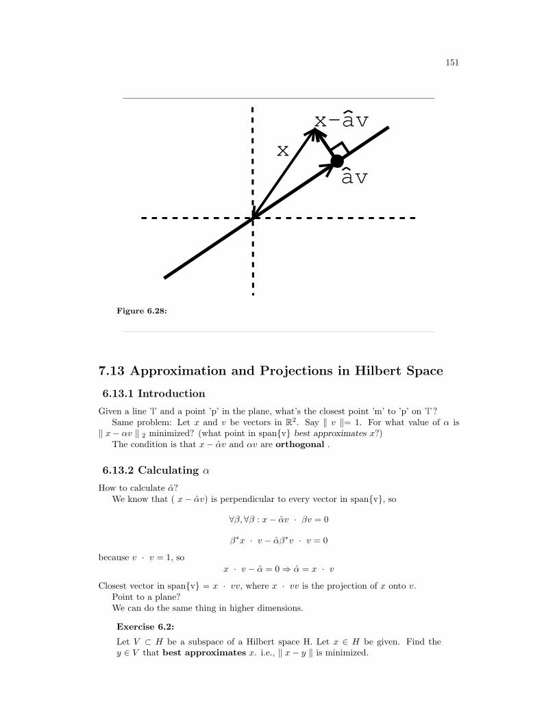
151
xx-av
av
Figure 6.28:
7.13 Approximation and Projections in Hilbert Space
6.13.1 Introduction
Given a line ’l’ and a point ’p’ in the plane, what’s the closest point ’m’ to ’p’ on ’l’?Same problem: Let x and v be vectors in R2. Say ‖ v ‖= 1. For what value of α is
‖ x− αv ‖ 2 minimized? (what point in spanv best approximates x?)The condition is that x− αv and αv are orthogonal .
6.13.2 Calculating α
How to calculate α?We know that ( x− αv) is perpendicular to every vector in spanv, so
∀β, ∀β : x− αv · βv = 0
β∗x · v − αβ∗v · v = 0
because v · v = 1, sox · v − α = 0 ⇒ α = x · v
Closest vector in spanv = x · vv, where x · vv is the projection of x onto v.Point to a plane?We can do the same thing in higher dimensions.
Exercise 6.2:
Let V ⊂ H be a subspace of a Hilbert space H. Let x ∈ H be given. Find they ∈ V that best approximates x. i.e., ‖ x− y ‖ is minimized.
152 CHAPTER 6. HILBERT SPACES AND ORTHOGONAL EXPANSIONS
Figure 6.29:
Solution:
1.- Find an orthonormal basis (Section 6.7.3) b1, . . . , bk for V2.- Project x onto V using
y =k∑
i=1
(x · bibi)
then y is the closest point in V to x and (x-y) ⊥ V ( ∀v,∀v ∈ V : x−y · v = 0
Example 6.24:
x ∈ R3, V = span
1
00
,
010
, x =
abc
. So,
y =2∑
i=1
(x · bibi) = a
100
+ b
010
=
ab0
Example 6.25:
V = space of periodic signals with frequency no greater than 3w0. Given periodicf(t), what is the signal in V that best approximates f?
1.- 1√Tejw0kt, k = -3, -2, ..., 2, 3 is an ONB for V
2.- g (t) = 1T
∑3k=−3
(f (t) · ejw0ktejw0kt
)is the closest signal in V to f(t) ⇒
reconstruct f(t) using only 7 terms of its Fourier series.
Example 6.26:
Let V = functions piecewise constant between the integers
1.- ONB for V.
bi =
1 if i− 1 ≤ t < i0 otherwise
where bi is an ONB.
Best piecewise constant approximation?
g (t) =∞∑
i=−∞(f · bibi)
f · bi =∫ ∞
−∞f (t) bi (t) dt =
∫ i
i−1
f (t) dt
Chapter 7
Fourier Analysis on ComplexSpaces
8.1 Fourier Analysis
Fourier analysis is fundamental to understanding the behavior of signals and systems. This isa result of the fact that sinusoids are FIX ME - Eigenfunctions of linear, time-invariant (LTI)systems. This is to say that if we pass any particular sinusoid through a LTI system, we get ascaled version of that same sinusoid on the output. Then, since Fourier analysis allows us toredefine the signals in terms of sinusoids, all we need to do is determine how any given systemeffects all possible sinusoids (its transfer function) and we have a complete understandingof the system. Furthermore, since we are able to define the passage of sinusoids througha system as multiplication of that sinusoid by the transfer function at the same frequency,we can convert the passage of any signal through a system from convolution (in time) tomultiplication (in frequency). These ideas are what give Fourier analysis its power.
Now, after hopefully having sold you on the value of this method of analysis, we mustexamine exactly what we mean by Fourier analysis. The four Fourier transforms thatcomprise this analysis are the Fourier Series, Continuous-Time Fourier Transform, Discrete-Time Fourier Transform and Discrete Fourier Transform. For this module, we will viewthe Laplace Transform and Z-Transform as simply extensions of the CTFT and DTFTrespectively. All of these transforms act essentially the same way, by converting a signalin time to an equivalent signal in frequency (sinusoids). However, depending on the natureof a specific signal (ie whether it is finite- or infinite-length and whether it is discrete- orcontinuous-time) there is an appropriate transform to convert the signal into the frequencydomain. Below is a table of the four Fourier transforms and when each is appropriate. Italso includes the relevant convolution for the specified space.
153
154 CHAPTER 7. FOURIER ANALYSIS ON COMPLEX SPACES
Table of Fourier Representations
Transform Time Domain Frequency Domain ConvolutionContinuous-TimeFourier Series
L2 ([0, T )) l2 (Z) Continuous-TimeCircular
Continuous-TimeFourier Transform
L2 (R) L2 (R) Continuous-TimeLinear
Discrete-TimeFourier Transform
l2 (Z) L2 ([0, 2π)) Discrete-Time Lin-ear
Discrete FourierTransform
l2 ([0, N − 1]) l2 ([0, N − 1]) Discrete-Time Cir-cular
8.2 Fourier Analysis in Complex Spaces
7.2.1 Introduction
By now you should be familiar with the derivation of the Fourier series for continuous-time,periodic functions. This derivation leads us to the following equations that you should bequite familiar with:
f (t) =∑
n
(cne
jω0nt)
(7.1)
cn = 1T
∫n
f (t) e−(jω0nt)dt
= 1T f · ejω0nt
(7.2)
where cn tells us the amount of frequency ω0n in f (t).In this module, we will derive a similar expansion for discrete-time, periodic functions.
In doing so, we will derive the Discrete Time Fourier Series (DTFS), or the DiscreteFourier Transform (DFT).
7.2.2 Derivation of DTFS
Much like a periodic, continuous-time function can be thought of as a function on the interval[0, T ]
A periodic, discrete-time signal (with period N) can be thought of as a finite set ofnumbers. For example, say we have the following set of numbers that describe a periodic,discrete-time signal, where N = 4:
. . . , 3, 2,−2, 1, 3, . . .
We can represent this signal as either a periodic signal or as just a single interval as follows:
note: The set of discrete time signals with period N equal CN .
Just like the continuous case, we are going to form a basis using harmonic sinusoids .Before we look into this, it will be worth our time to look at the discrete-time, complexsinusoids in a little more detail.
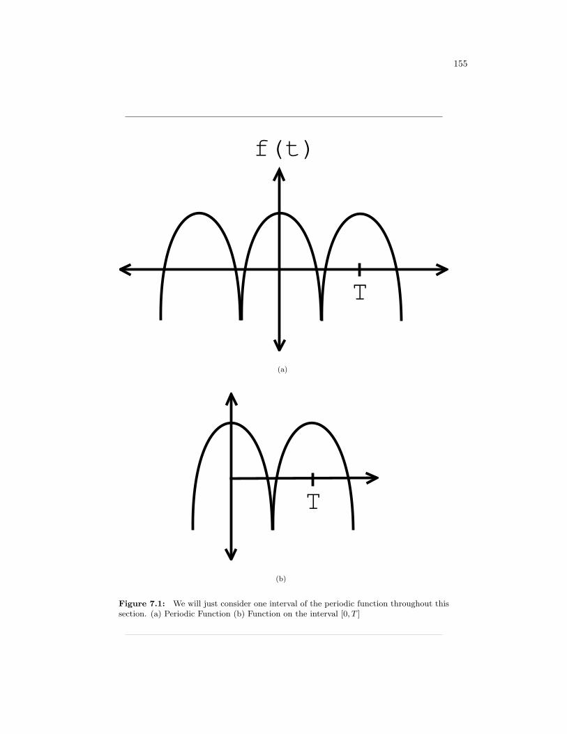
155
T
f(t)
(a)
T
(b)
Figure 7.1: We will just consider one interval of the periodic function throughout thissection. (a) Periodic Function (b) Function on the interval [0, T ]
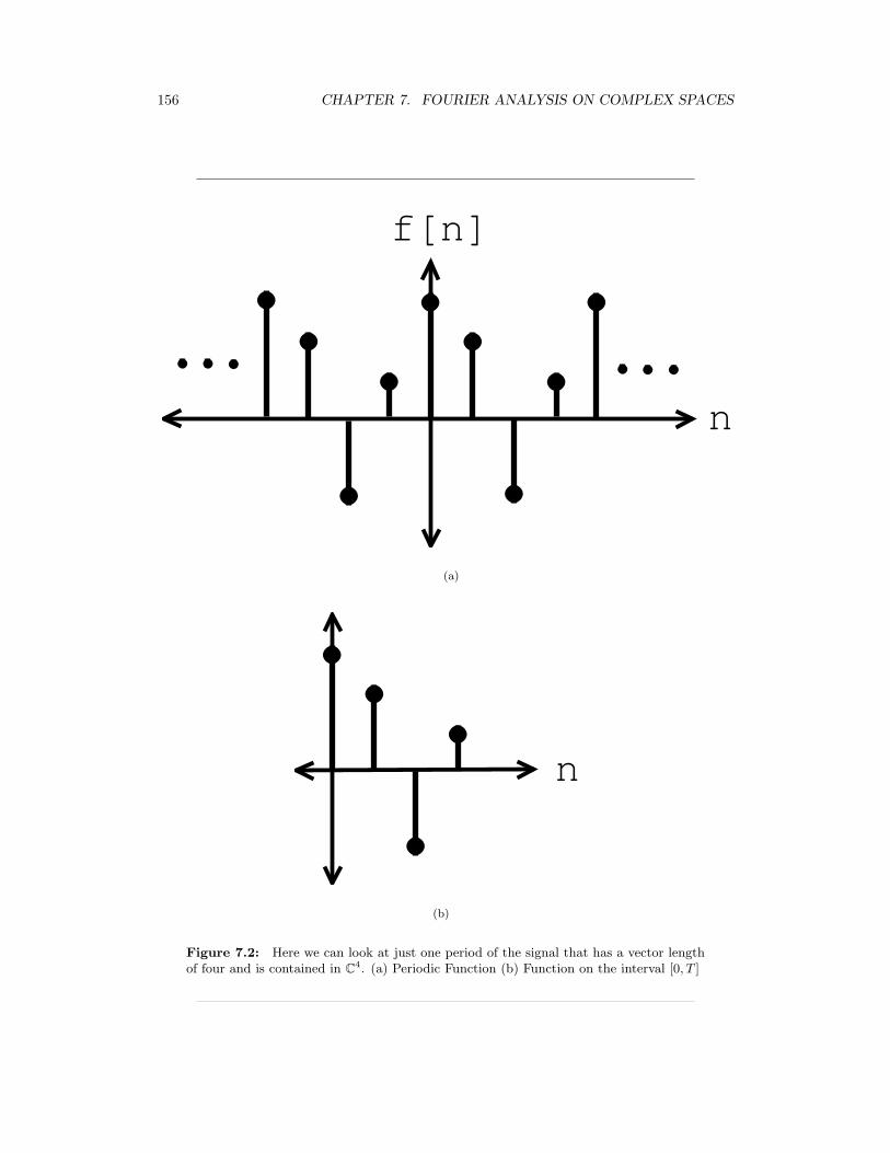
156 CHAPTER 7. FOURIER ANALYSIS ON COMPLEX SPACES
f[n]
n
(a)
n
(b)
Figure 7.2: Here we can look at just one period of the signal that has a vector lengthof four and is contained in C4. (a) Periodic Function (b) Function on the interval [0, T ]
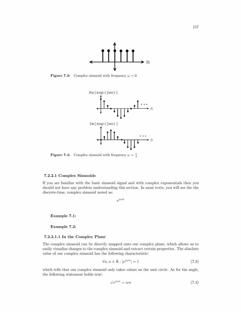
157
Figure 7.3: Complex sinusoid with frequency ω = 0
Figure 7.4: Complex sinusoid with frequency ω = π4
7.2.2.1 Complex Sinusoids
If you are familiar with the basic sinusoid signal and with complex exponentials then youshould not have any problem understanding this section. In most texts, you will see the thediscrete-time, complex sinusoid noted as:
ejωn
Example 7.1:
Example 7.2:
7.2.2.1.1 In the Complex Plane
The complex sinusoid can be directly mapped onto our complex plane, which allows us toeasily visualize changes to the complex sinusoid and extract certain properties. The absolutevalue of our complex sinusoid has the following characteristic:
∀n, n ∈ R : |ejωn| = 1 (7.3)
which tells that our complex sinusoid only takes values on the unit circle. As for the angle,the following statement holds true:
∠ejωn = wn (7.4)
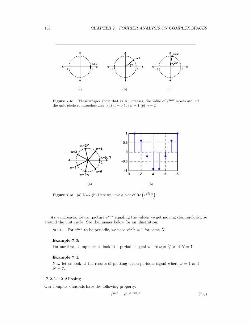
158 CHAPTER 7. FOURIER ANALYSIS ON COMPLEX SPACES
(a) (b) (c)
Figure 7.5: These images show that as n increases, the value of ejωn moves aroundthe unit circle counterclockwise. (a) n = 0 (b) n = 1 (c) n = 2
(a) (b)
Figure 7.6: (a) N=7 (b) Here we have a plot of Re(ej 2π
7 n).
As n increases, we can picture ejωn equaling the values we get moving counterclockwisearound the unit circle. See the images below for an illustration:
note: For ejωn to be periodic, we need ejωN = 1 for some N .
Example 7.3:
For our first example let us look at a periodic signal where ω = 2π7 and N = 7.
Example 7.4:
Now let us look at the results of plotting a non-periodic siganl where ω = 1 andN = 7.
7.2.2.1.2 Aliasing
Our complex sinusoids have the following property:
ejωn = ej(ω+2π)n (7.5)
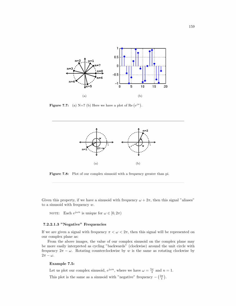
159
(a) (b)
Figure 7.7: (a) N=7 (b) Here we have a plot of Re(ejn
).
(a) (b)
Figure 7.8: Plot of our complex sinusoid with a frequency greater than pi.
Given this property, if we have a sinusoid with frequency ω + 2π, then this signal ”aliases”to a sinusoid with frequency w.
note: Each ejωn is unique for ω ∈ [0, 2π)
7.2.2.1.3 ”Negative” Frequencies
If we are given a signal with frequency π < ω < 2π, then this signal will be represented onour complex plane as:
From the above images, the value of our complex sinusoid on the complex plane maybe more easily interpreted as cycling ”backwards” (clockwise) around the unit circle withfrequency 2π − ω. Rotating counterclockwise by w is the same as rotating clockwise by2π − ω.
Example 7.5:
Let us plot our complex sinusoid, ejωn, where we have ω = 5π4 and n = 1.
This plot is the same as a sinusoid with ”negative” frequency −(
3π4
).
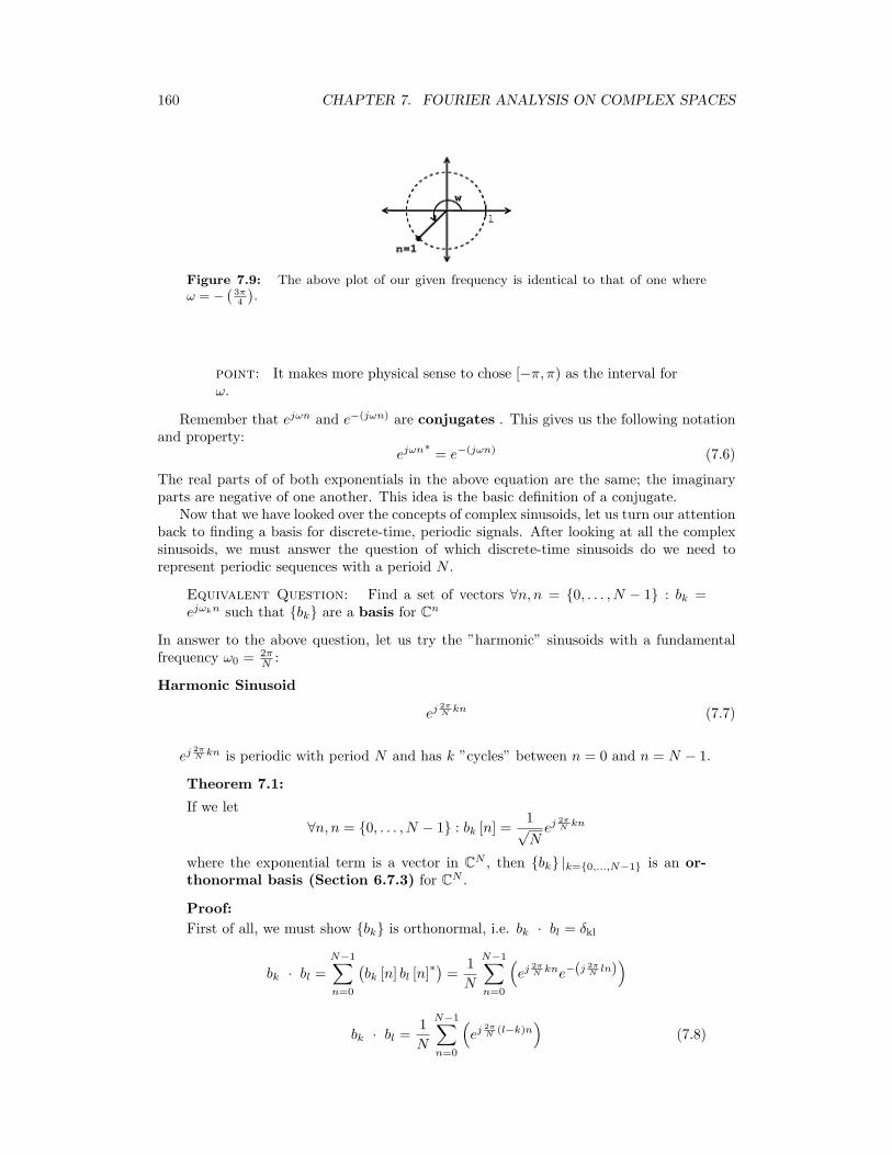
160 CHAPTER 7. FOURIER ANALYSIS ON COMPLEX SPACES
Figure 7.9: The above plot of our given frequency is identical to that of one whereω = −
(3π4
).
point: It makes more physical sense to chose [−π, π) as the interval forω.
Remember that ejωn and e−(jωn) are conjugates . This gives us the following notationand property:
ejωn∗ = e−(jωn) (7.6)
The real parts of of both exponentials in the above equation are the same; the imaginaryparts are negative of one another. This idea is the basic definition of a conjugate.
Now that we have looked over the concepts of complex sinusoids, let us turn our attentionback to finding a basis for discrete-time, periodic signals. After looking at all the complexsinusoids, we must answer the question of which discrete-time sinusoids do we need torepresent periodic sequences with a perioid N .
Equivalent Question: Find a set of vectors ∀n, n = 0, . . . , N − 1 : bk =ejωkn such that bk are a basis for Cn
In answer to the above question, let us try the ”harmonic” sinusoids with a fundamentalfrequency ω0 = 2π
N :
Harmonic Sinusoid
ej 2πN kn (7.7)
ej 2πN kn is periodic with period N and has k ”cycles” between n = 0 and n = N − 1.
Theorem 7.1:
If we let∀n, n = 0, . . . , N − 1 : bk [n] =
1√Nej 2π
N kn
where the exponential term is a vector in CN , then bk |k=0,...,N−1 is an or-thonormal basis (Section 6.7.3) for CN .
Proof:First of all, we must show bk is orthonormal, i.e. bk · bl = δkl
bk · bl =N−1∑n=0
(bk [n] bl [n]∗
)=
1N
N−1∑n=0
(ej 2π
N kne−(j 2πN ln)
)
bk · bl =1N
N−1∑n=0
(ej 2π
N (l−k)n)
(7.8)
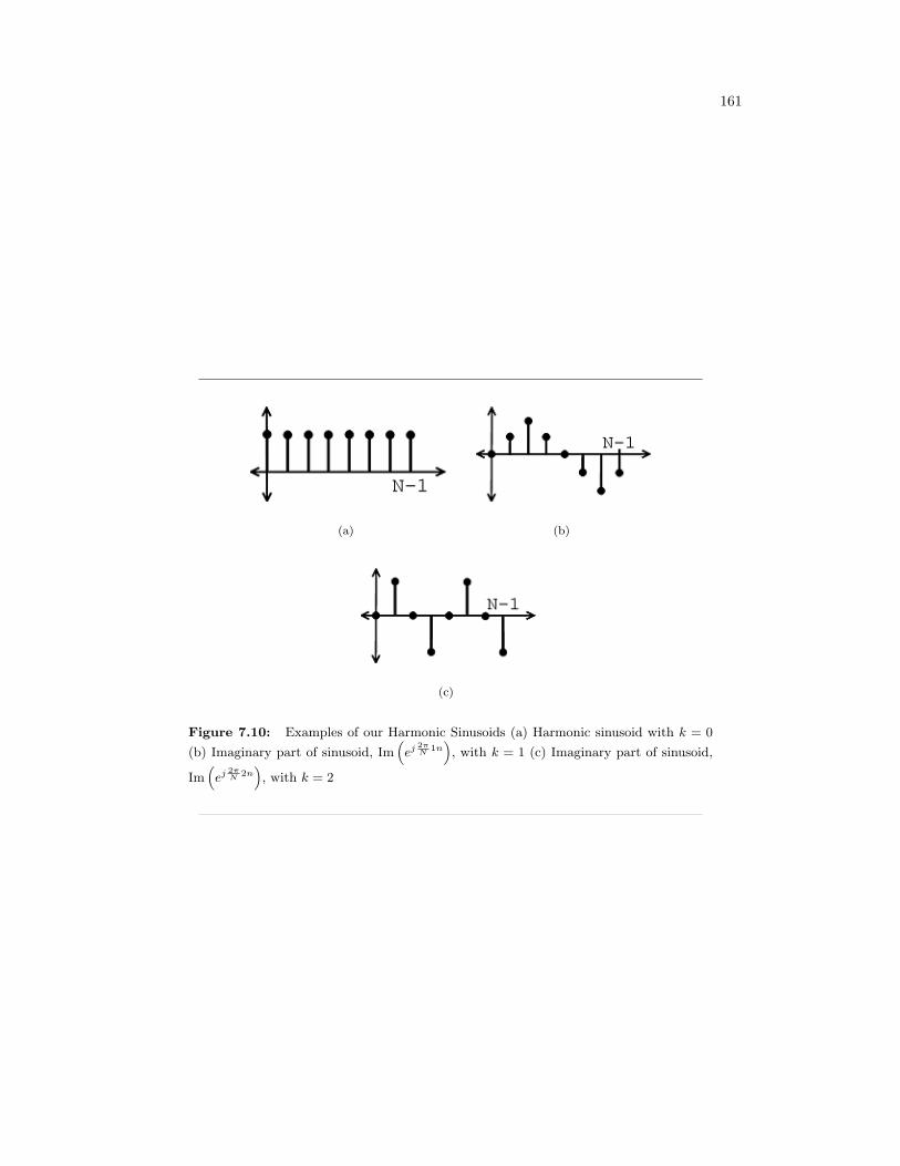
161
(a) (b)
(c)
Figure 7.10: Examples of our Harmonic Sinusoids (a) Harmonic sinusoid with k = 0
(b) Imaginary part of sinusoid, Im(ej 2π
N1n
), with k = 1 (c) Imaginary part of sinusoid,
Im(ej 2π
N2n
), with k = 2
162 CHAPTER 7. FOURIER ANALYSIS ON COMPLEX SPACES
If l = k, thenbk · bl = 1
N
∑N−1n=0 (1)
= 1(7.9)
If l 6= k, then we must use the ”partial summation formula” shown below:
N−1∑n=0
(αn) =∞∑
n=0
(αn)−∞∑
n=N
(αn) =1
1− α− αN
1− α=
1− αN
1− α
bk · bl =1N
N−1∑n=0
(ej 2π
N (l−k)n)
where in the above equation we can say that α = ej 2πN (l−k), and thus we can see
how this is in the form needed to utilize our partial summation formula.
bk · bl =1N
(1− ej 2π
N (l−k)N
1− ej 2πN (l−k)
)=
1N
(1− 1
1− ej 2πN (l−k)
)= 0
So,
bk · bl =
1 if k = l0 if k 6= l
(7.10)
Therefore: bk is an orthonormal set. bk is also a basis (Section 4.1.3), sincethere are N vectors which are linearly independent (Section 4.1.1) (orthoganalityimplies linear independence).
And finally, we have shown that the harmonic sinusoids
1√Nej 2π
N kn
form anorthonormal basis for Cn
7.2.2.2 Discrete-Time Fourier Series (DTFS)
Using the steps shown above in the derivation and our previous understanding of HilbertSpaces and Orthogonal Expansions, the rest of the derivation is automatic. Given a discrete-time, periodic signal (vector in Cn) f [n], we can write:
f [n] =1√N
N−1∑k=0
(cke
j 2πN kn
)(7.11)
ck =1√N
N−1∑n=0
(f [n] e−(j 2π
N kn))
(7.12)
Note: Most people collect both the 1√N
terms into the expression for ck.
Discrete Time Fourier Series: Here is the common form of the DTFS withthe above note taken into account:
f [n] =N−1∑k=0
(cke
j 2πN kn
)
ck =1N
N−1∑n=0
(f [n] e−(j 2π
N kn))
This what the fft command in MATLAB does.
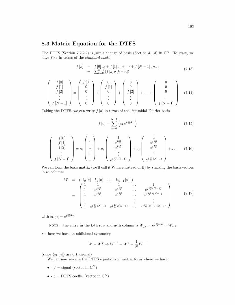
163
8.3 Matrix Equation for the DTFS
The DTFS (Section 7.2.2.2) is just a change of basis (Section 4.1.3) in CN . To start, wehave f [n] in terms of the standard basis.
f [n] = f [0] e0 + f [1] e1 + · · ·+ f [N − 1] eN−1
=∑n−1
k=0 (f [k] δ [k − n])(7.13)
f [0]f [1]f [2]
...f [N − 1]
=
f [0]00...0
+
0
f [1]0...0
+
00
f [2]...0
+ · · ·+
000...
f [N − 1]
(7.14)
Taking the DTFS, we can write f [n] in terms of the sinusoidal Fourier basis
f [n] =N−1∑k=0
(cke
j 2πN kn
)(7.15)
f [0]f [1]f [2]
...f [N − 1]
= c0
111...1
+ c1
1
ej 2πN
ej 4πN
...ej 2π
N (N−1)
+ c2
1
ej 4πN
ej 8πN
...ej 4π
N (N−1)
+ . . . (7.16)
We can form the basis matrix (we’ll call it W here instead of B) by stacking the basis vectorsin as columns
W =(b0 [n] b1 [n] . . . bN−1 [n]
)
=
1 1 1 . . . 11 ej 2π
N ej 4πN . . . ej 2π
N (N−1)
1 ej 4πN ej 8π
N . . . ej 2πN 2(N−1)
......
......
...1 ej 2π
N (N−1) ej 2πN 2(N−1) . . . ej 2π
N (N−1)(N−1)
(7.17)
with bk [n] = ej 2πN kn
note: the entry in the k-th row and n-th column is Wj,k = ej 2πN kn = Wn,k
So, here we have an additional symmetry
W = WT ⇒WT ∗ = W ∗ =1NW−1
(since bk [n] are orthogonal)We can now rewrite the DTFS equations in matrix form where we have:
• - f = signal (vector in CN )
• - c = DTFS coeffs. (vector in CN )
164 CHAPTER 7. FOURIER ANALYSIS ON COMPLEX SPACES
”synthesis” f = Wc f [n] = c · bn∗
”analysis” c = WT ∗f = W ∗f c [k] = f · bk
Finding (and inverting) the DTFS is just matrix multiplication.Everything in CN is clean: no limits, no convergence questions, just good ole matrix
arithmetic.
8.4 Periodic Extension to DTFS
7.4.1 Introduction
Now that we have an understanding of the discrete-time Fourier series (DTFS) (Section 7.2.2.2),we can consider the periodic extension of c [k] (the Discrete-time Fourier coefficients). Thebasic figures below show a simple illustration of how we can represent a sequence as aperiodic signal mapped over an infinite number of intervals.
Exercise 7.1:
Why does a periodic extension to the DTFS coefficients c [k] make sense?
Solution:Aliasing: bk = ej 2π
N kn
bk+N = ej 2πN (k+N)n
= ej 2πN knej2πn
= ej 2πN n
= bk
(7.18)
→ DTFS coefficients are also periodic with period N.
7.4.2 Examples
Example 7.6: Discrete time square wave
Calculate the DTFS c [k] using:
c [k] =1N
N−1∑n=0
(f [n] e−(j 2π
N kn))
(7.19)
Just like continuous time Fourier series, we can take the summation over anyinterval, so we have
ck =1N
N1∑n=−N1
(e−(j 2π
N kn))
(7.20)
Let m = n+N1 (so we can get a geometric series starting at 0)
ck = 1N
∑2N1m=0
(e−(j 2π
N (m−N1)k))
= 1N e
j 2πN k∑2N1
m=0
(e−(j 2π
N mk)) (7.21)
Now, using the ”partial summation formula”
M∑n=0
(an) =1− aM+1
1− a(7.22)
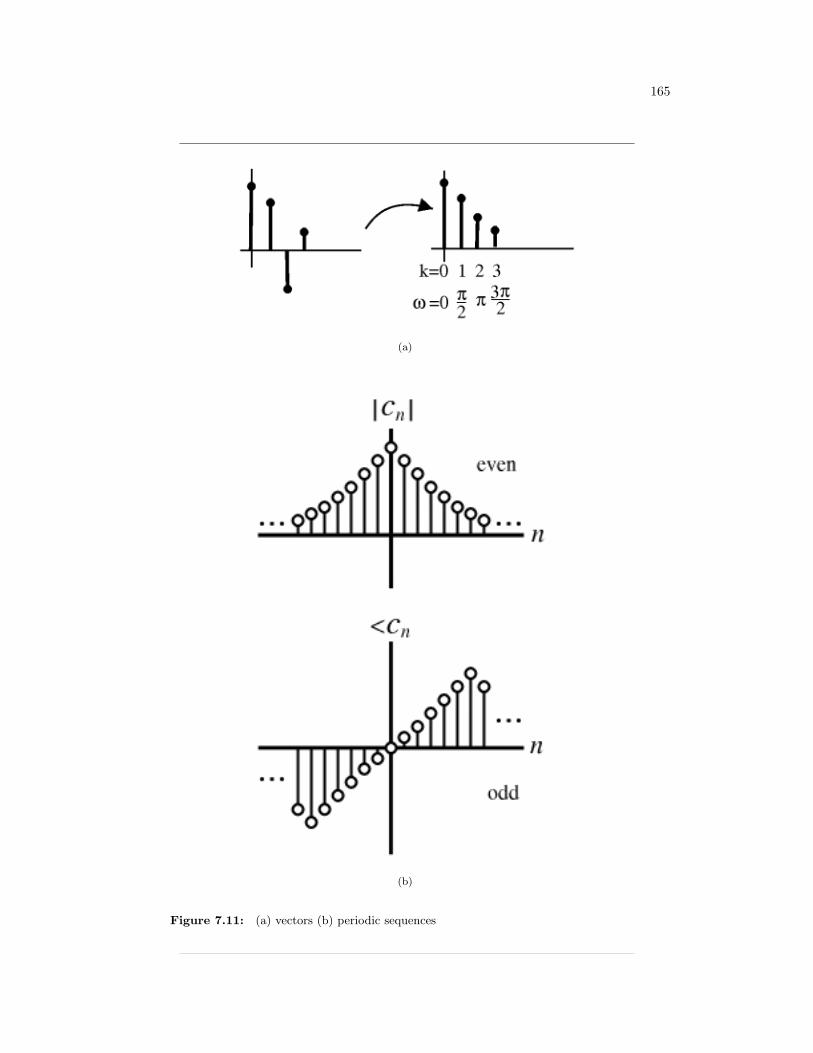
165
(a)
(b)
Figure 7.11: (a) vectors (b) periodic sequences
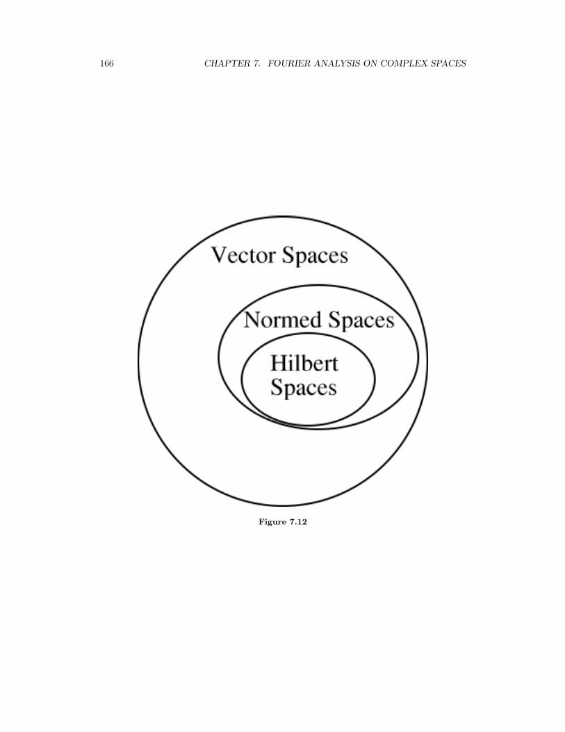
166 CHAPTER 7. FOURIER ANALYSIS ON COMPLEX SPACES
Figure 7.12
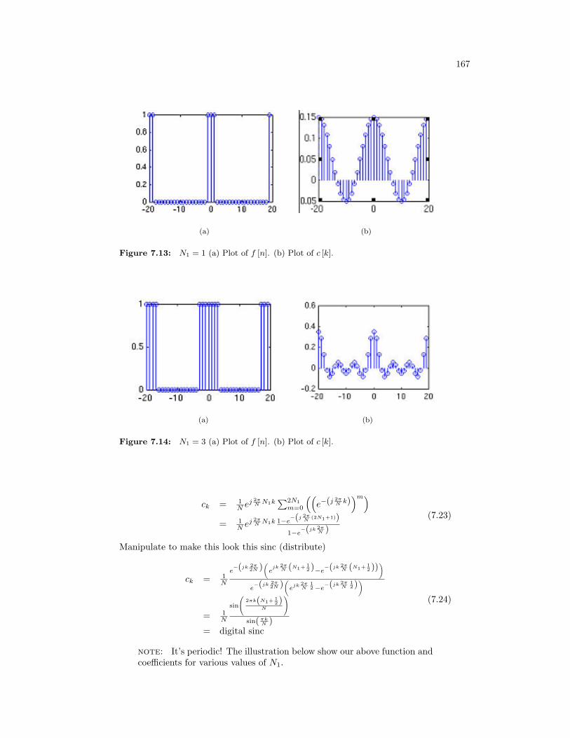
167
(a) (b)
Figure 7.13: N1 = 1 (a) Plot of f [n]. (b) Plot of c [k].
(a) (b)
Figure 7.14: N1 = 3 (a) Plot of f [n]. (b) Plot of c [k].
ck = 1N e
j 2πN N1k
∑2N1m=0
((e−(j 2π
N k))m)
= 1N e
j 2πN N1k 1−e
−(j 2πN
(2N1+1))
1−e−(jk 2π
N )(7.23)
Manipulate to make this look this sinc (distribute)
ck = 1N
e−(jk 2π
2N )(
ejk 2π
N (N1+ 12 )−e
−(jk 2πN (N1+ 1
2 )))
e−(jk 2π
2N )(
ejk 2πN
12−e
−(jk 2πN
12 ))
= 1N
sin
(2πk(N1+ 1
2 )N
)sin(πk
N )= digital sinc
(7.24)
note: It’s periodic! The illustration below show our above function andcoefficients for various values of N1.
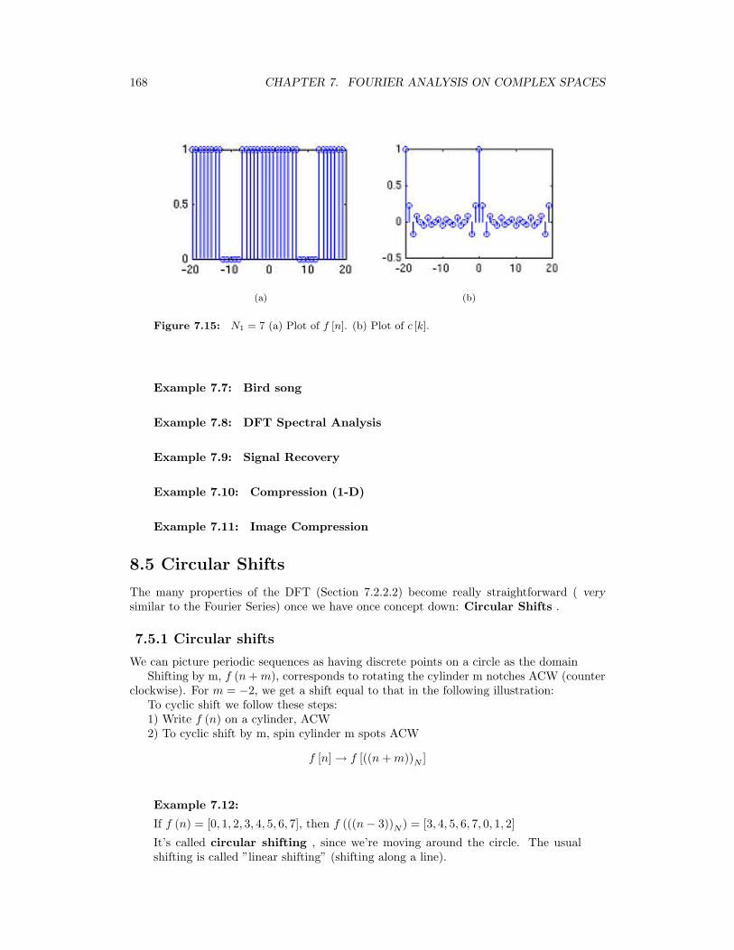
168 CHAPTER 7. FOURIER ANALYSIS ON COMPLEX SPACES
(a) (b)
Figure 7.15: N1 = 7 (a) Plot of f [n]. (b) Plot of c [k].
Example 7.7: Bird song
Example 7.8: DFT Spectral Analysis
Example 7.9: Signal Recovery
Example 7.10: Compression (1-D)
Example 7.11: Image Compression
8.5 Circular Shifts
The many properties of the DFT (Section 7.2.2.2) become really straightforward ( verysimilar to the Fourier Series) once we have once concept down: Circular Shifts .
7.5.1 Circular shifts
We can picture periodic sequences as having discrete points on a circle as the domainShifting by m, f (n+m), corresponds to rotating the cylinder m notches ACW (counter
clockwise). For m = −2, we get a shift equal to that in the following illustration:To cyclic shift we follow these steps:1) Write f (n) on a cylinder, ACW2) To cyclic shift by m, spin cylinder m spots ACW
f [n] → f [((n+m))N ]
Example 7.12:
If f (n) = [0, 1, 2, 3, 4, 5, 6, 7], then f (((n− 3))N ) = [3, 4, 5, 6, 7, 0, 1, 2]
It’s called circular shifting , since we’re moving around the circle. The usualshifting is called ”linear shifting” (shifting along a line).

169
Figure 7.16

170 CHAPTER 7. FOURIER ANALYSIS ON COMPLEX SPACES
Figure 7.17

171
Figure 7.18

172 CHAPTER 7. FOURIER ANALYSIS ON COMPLEX SPACES
Figure 7.19

173
(a)
(b)
Figure 7.20: We’ve cut down on storage space by >90% (while incurring some loss) (a)256 by 256 image (65,636 pixels) (b) Reconstructed using only 6000 coefficients
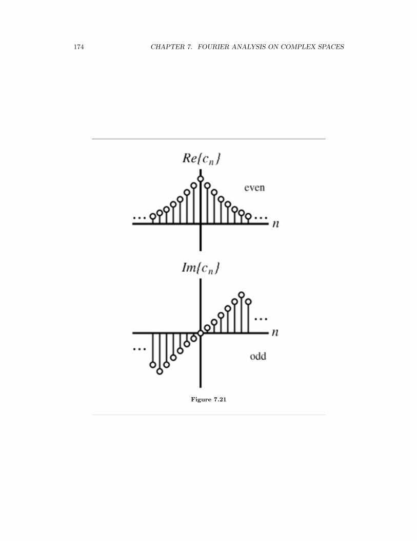
174 CHAPTER 7. FOURIER ANALYSIS ON COMPLEX SPACES
Figure 7.21
175
Figure 7.22: for m = −2
Figure 7.23
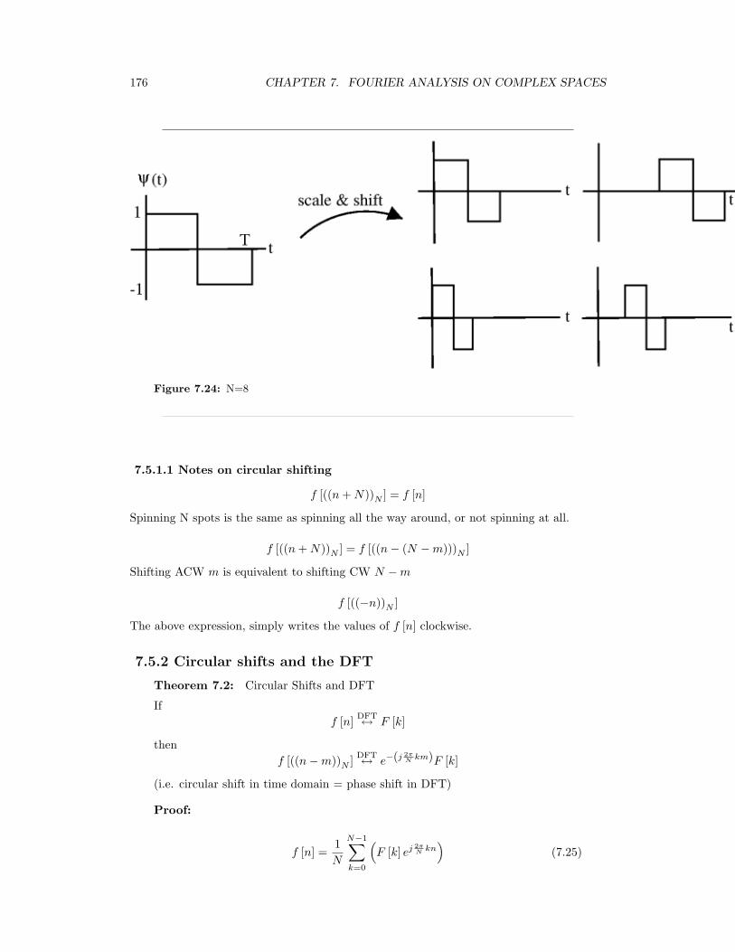
176 CHAPTER 7. FOURIER ANALYSIS ON COMPLEX SPACES
Figure 7.24: N=8
7.5.1.1 Notes on circular shifting
f [((n+N))N ] = f [n]
Spinning N spots is the same as spinning all the way around, or not spinning at all.
f [((n+N))N ] = f [((n− (N −m)))N ]
Shifting ACW m is equivalent to shifting CW N −m
f [((−n))N ]
The above expression, simply writes the values of f [n] clockwise.
7.5.2 Circular shifts and the DFT
Theorem 7.2: Circular Shifts and DFT
Iff [n] DFT↔ F [k]
thenf [((n−m))N ] DFT↔ e−(j 2π
N km)F [k]
(i.e. circular shift in time domain = phase shift in DFT)
Proof:
f [n] =1N
N−1∑k=0
(F [k] ej 2π
N kn)
(7.25)
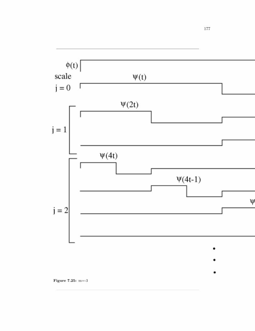
177
Figure 7.25: m=-3
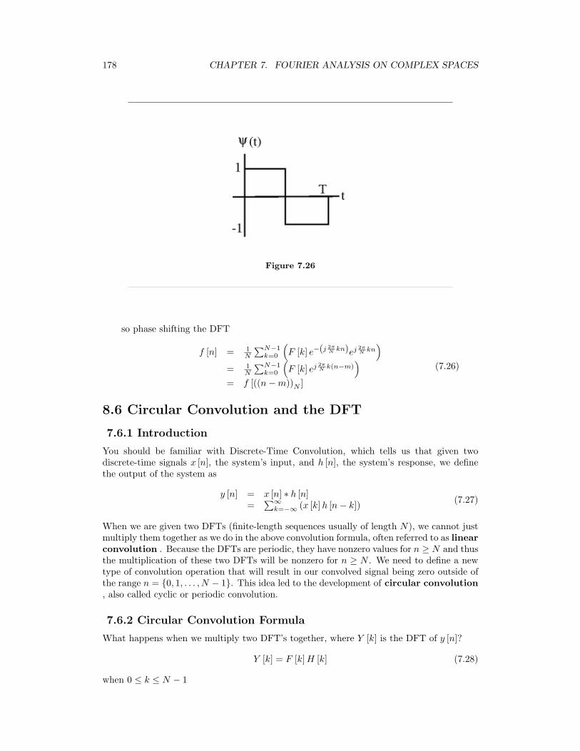
178 CHAPTER 7. FOURIER ANALYSIS ON COMPLEX SPACES
Figure 7.26
so phase shifting the DFT
f [n] = 1N
∑N−1k=0
(F [k] e−(j 2π
N kn)ej 2πN kn
)= 1
N
∑N−1k=0
(F [k] ej 2π
N k(n−m))
= f [((n−m))N ]
(7.26)
8.6 Circular Convolution and the DFT
7.6.1 Introduction
You should be familiar with Discrete-Time Convolution, which tells us that given twodiscrete-time signals x [n], the system’s input, and h [n], the system’s response, we definethe output of the system as
y [n] = x [n] ∗ h [n]=
∑∞k=−∞ (x [k]h [n− k]) (7.27)
When we are given two DFTs (finite-length sequences usually of length N), we cannot justmultiply them together as we do in the above convolution formula, often referred to as linearconvolution . Because the DFTs are periodic, they have nonzero values for n ≥ N and thusthe multiplication of these two DFTs will be nonzero for n ≥ N . We need to define a newtype of convolution operation that will result in our convolved signal being zero outside ofthe range n = 0, 1, . . . , N − 1. This idea led to the development of circular convolution, also called cyclic or periodic convolution.
7.6.2 Circular Convolution Formula
What happens when we multiply two DFT’s together, where Y [k] is the DFT of y [n]?
Y [k] = F [k]H [k] (7.28)
when 0 ≤ k ≤ N − 1
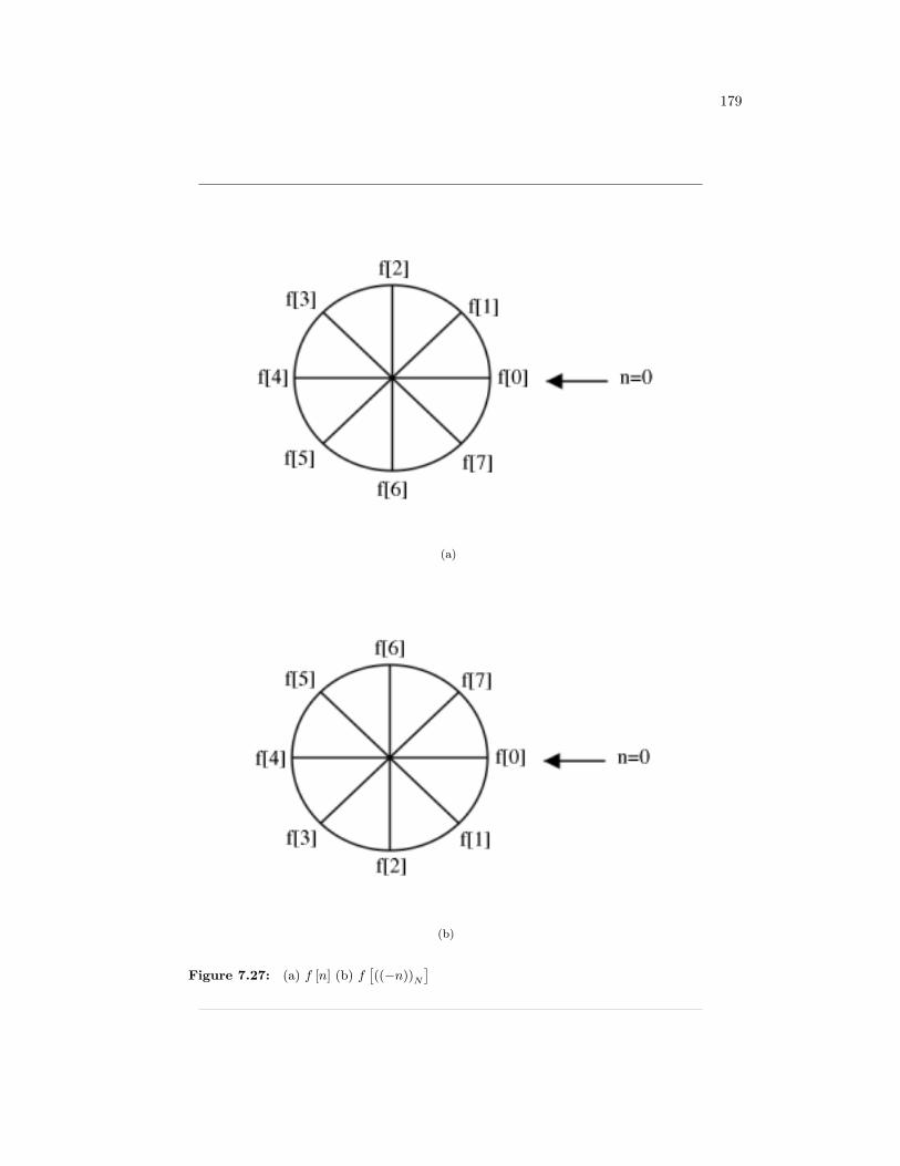
179
(a)
(b)
Figure 7.27: (a) f [n] (b) f[((−n))N
]
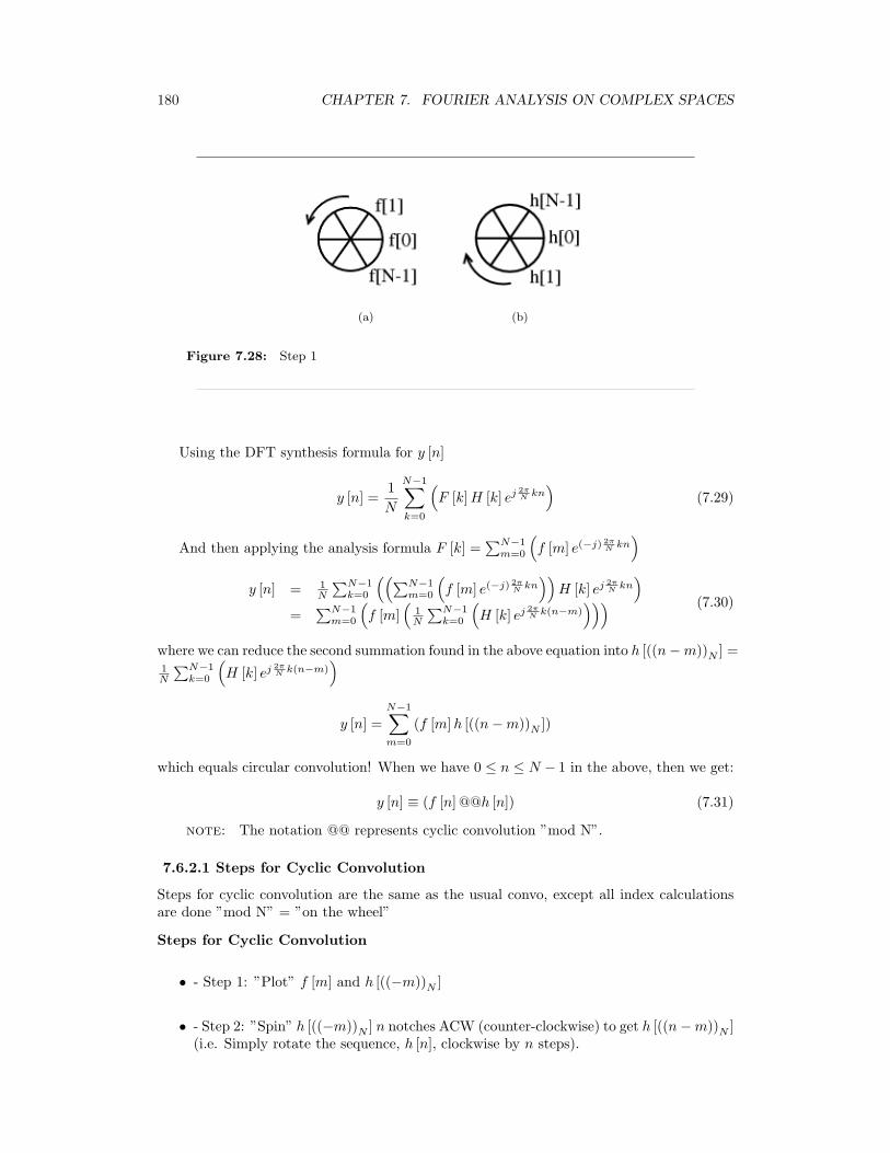
180 CHAPTER 7. FOURIER ANALYSIS ON COMPLEX SPACES
(a) (b)
Figure 7.28: Step 1
Using the DFT synthesis formula for y [n]
y [n] =1N
N−1∑k=0
(F [k]H [k] ej 2π
N kn)
(7.29)
And then applying the analysis formula F [k] =∑N−1
m=0
(f [m] e(−j) 2π
N kn)
y [n] = 1N
∑N−1k=0
((∑N−1m=0
(f [m] e(−j) 2π
N kn))
H [k] ej 2πN kn
)=
∑N−1m=0
(f [m]
(1N
∑N−1k=0
(H [k] ej 2π
N k(n−m)))) (7.30)
where we can reduce the second summation found in the above equation into h [((n−m))N ] =1N
∑N−1k=0
(H [k] ej 2π
N k(n−m))y [n] =
N−1∑m=0
(f [m]h [((n−m))N ])
which equals circular convolution! When we have 0 ≤ n ≤ N − 1 in the above, then we get:
y [n] ≡ (f [n] @@h [n]) (7.31)
note: The notation @@ represents cyclic convolution ”mod N”.
7.6.2.1 Steps for Cyclic Convolution
Steps for cyclic convolution are the same as the usual convo, except all index calculationsare done ”mod N” = ”on the wheel”
Steps for Cyclic Convolution
• - Step 1: ”Plot” f [m] and h [((−m))N ]
• - Step 2: ”Spin” h [((−m))N ] n notches ACW (counter-clockwise) to get h [((n−m))N ](i.e. Simply rotate the sequence, h [n], clockwise by n steps).
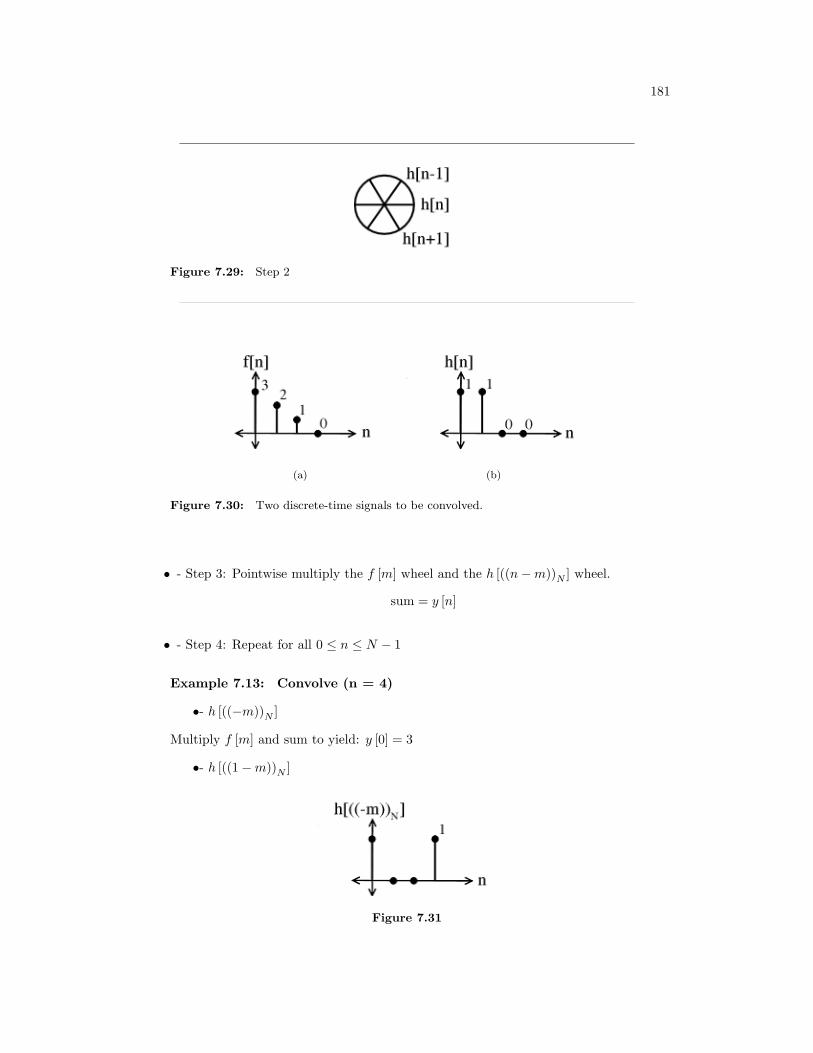
181
Figure 7.29: Step 2
(a) (b)
Figure 7.30: Two discrete-time signals to be convolved.
• - Step 3: Pointwise multiply the f [m] wheel and the h [((n−m))N ] wheel.
sum = y [n]
• - Step 4: Repeat for all 0 ≤ n ≤ N − 1
Example 7.13: Convolve (n = 4)
•- h [((−m))N ]
Multiply f [m] and sum to yield: y [0] = 3
•- h [((1−m))N ]
Figure 7.31
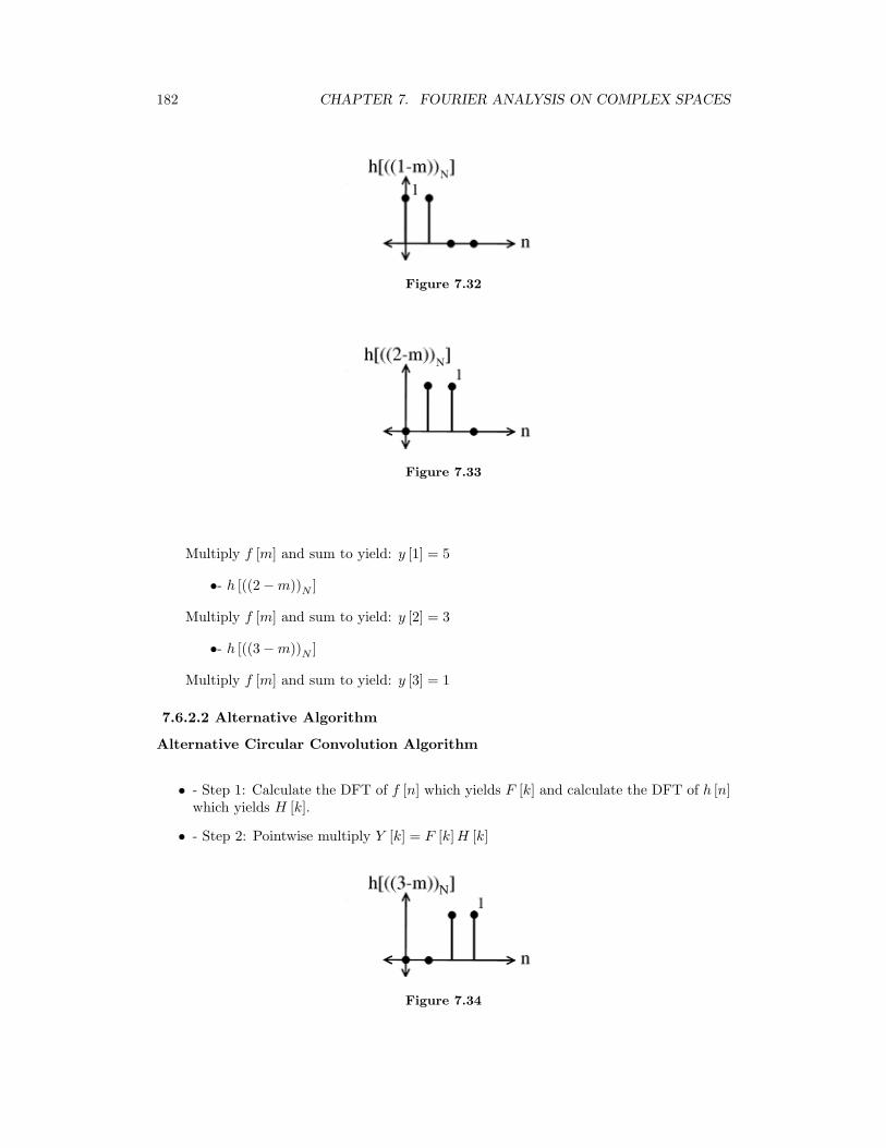
182 CHAPTER 7. FOURIER ANALYSIS ON COMPLEX SPACES
Figure 7.32
Figure 7.33
Multiply f [m] and sum to yield: y [1] = 5
•- h [((2−m))N ]
Multiply f [m] and sum to yield: y [2] = 3
•- h [((3−m))N ]
Multiply f [m] and sum to yield: y [3] = 1
7.6.2.2 Alternative Algorithm
Alternative Circular Convolution Algorithm
• - Step 1: Calculate the DFT of f [n] which yields F [k] and calculate the DFT of h [n]which yields H [k].
• - Step 2: Pointwise multiply Y [k] = F [k]H [k]
Figure 7.34
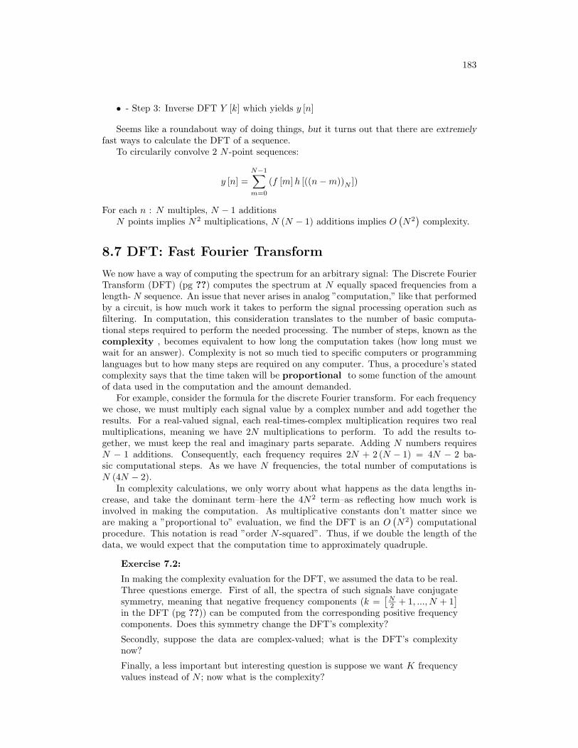
183
• - Step 3: Inverse DFT Y [k] which yields y [n]
Seems like a roundabout way of doing things, but it turns out that there are extremelyfast ways to calculate the DFT of a sequence.
To circularily convolve 2 N -point sequences:
y [n] =N−1∑m=0
(f [m]h [((n−m))N ])
For each n : N multiples, N − 1 additionsN points implies N2 multiplications, N (N − 1) additions implies O
(N2)
complexity.
8.7 DFT: Fast Fourier Transform
We now have a way of computing the spectrum for an arbitrary signal: The Discrete FourierTransform (DFT) (pg ??) computes the spectrum at N equally spaced frequencies from alength- N sequence. An issue that never arises in analog ”computation,” like that performedby a circuit, is how much work it takes to perform the signal processing operation such asfiltering. In computation, this consideration translates to the number of basic computa-tional steps required to perform the needed processing. The number of steps, known as thecomplexity , becomes equivalent to how long the computation takes (how long must wewait for an answer). Complexity is not so much tied to specific computers or programminglanguages but to how many steps are required on any computer. Thus, a procedure’s statedcomplexity says that the time taken will be proportional to some function of the amountof data used in the computation and the amount demanded.
For example, consider the formula for the discrete Fourier transform. For each frequencywe chose, we must multiply each signal value by a complex number and add together theresults. For a real-valued signal, each real-times-complex multiplication requires two realmultiplications, meaning we have 2N multiplications to perform. To add the results to-gether, we must keep the real and imaginary parts separate. Adding N numbers requiresN − 1 additions. Consequently, each frequency requires 2N + 2 (N − 1) = 4N − 2 ba-sic computational steps. As we have N frequencies, the total number of computations isN (4N − 2).
In complexity calculations, we only worry about what happens as the data lengths in-crease, and take the dominant term–here the 4N2 term–as reflecting how much work isinvolved in making the computation. As multiplicative constants don’t matter since weare making a ”proportional to” evaluation, we find the DFT is an O
(N2)
computationalprocedure. This notation is read ”order N -squared”. Thus, if we double the length of thedata, we would expect that the computation time to approximately quadruple.
Exercise 7.2:
In making the complexity evaluation for the DFT, we assumed the data to be real.Three questions emerge. First of all, the spectra of such signals have conjugatesymmetry, meaning that negative frequency components (k =
[N2 + 1, ..., N + 1
]in the DFT (pg ??)) can be computed from the corresponding positive frequencycomponents. Does this symmetry change the DFT’s complexity?
Secondly, suppose the data are complex-valued; what is the DFT’s complexitynow?
Finally, a less important but interesting question is suppose we want K frequencyvalues instead of N ; now what is the complexity?
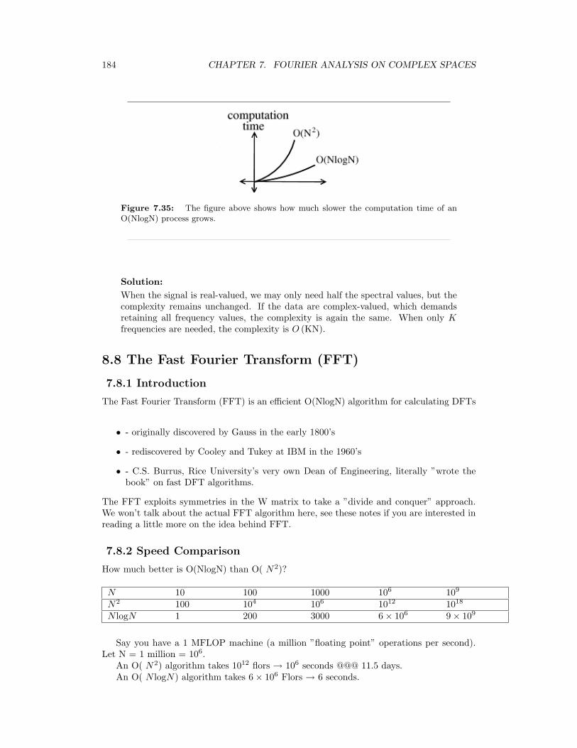
184 CHAPTER 7. FOURIER ANALYSIS ON COMPLEX SPACES
Figure 7.35: The figure above shows how much slower the computation time of anO(NlogN) process grows.
Solution:When the signal is real-valued, we may only need half the spectral values, but thecomplexity remains unchanged. If the data are complex-valued, which demandsretaining all frequency values, the complexity is again the same. When only Kfrequencies are needed, the complexity is O (KN).
8.8 The Fast Fourier Transform (FFT)
7.8.1 Introduction
The Fast Fourier Transform (FFT) is an efficient O(NlogN) algorithm for calculating DFTs
• - originally discovered by Gauss in the early 1800’s
• - rediscovered by Cooley and Tukey at IBM in the 1960’s
• - C.S. Burrus, Rice University’s very own Dean of Engineering, literally ”wrote thebook” on fast DFT algorithms.
The FFT exploits symmetries in the W matrix to take a ”divide and conquer” approach.We won’t talk about the actual FFT algorithm here, see these notes if you are interested inreading a little more on the idea behind FFT.
7.8.2 Speed Comparison
How much better is O(NlogN) than O( N2)?
N 10 100 1000 106 109
N2 100 104 106 1012 1018
N logN 1 200 3000 6× 10⁶ 9× 10⁹
Say you have a 1 MFLOP machine (a million ”floating point” operations per second).Let N = 1 million = 106.
An O( N2) algorithm takes 1012 flors → 106 seconds @@@ 11.5 days.An O( N logN) algorithm takes 6× 10⁶ Flors → 6 seconds.
185
note: N = 1 million is not unreasonable.
Example 7.14:
3 megapixel digital camera spits out 3× 10⁶ numbers for each picture. So for twoN point sequences f [n] and h [n]. If computing (f [n] @@h [n]) directly: O( N2)operations.
taking FFTs – O(NlogN)
multiplying FFTs – O(N)
inverse FFTs – O(NlogN).
the total complexity is O(NlogN).
note: FFT + digital computer were almost completely responsible forthe ”explosion” of DSP in the 60’s.
note: Rice was (and still is) one of the places to do research in DSP.
8.9 Deriving the Fast Fourier Transform
To derive the FFT, we assume that the signal’s duration is a power of two: N = 2l .Consider what happens to the even-numbered and odd-numbered elements of the sequencein the DFT calculation.
S (k) = s (0) + s (2) e(−j) 2π2kN + · · ·+ s (N − 2) e(−j)
2π(N−2)kN + s (1) e(−j) 2πk
N + s (3) e(−j)2π(2+1)k
N + · · ·+ s (N − 1) e(−j)2π(N−2+1)k
N
= s (0) + s (2) e(−j) 2πk
N2 + · · ·+ s (N − 2) e
(−j)2π(N
2 −1)k
N2 +
s (1) + s (3) e(−j) 2πk
N2 + · · ·+ s (N − 1) e
(−j)2π(N
2 −1)k
N2
e−(j2πk)
N
(7.32)Each term in square brackets has the form of a N
2 -length DFT. The first one is aDFT of the even-numbered elements, and the second of the odd-numbered elements. Thefirst DFT is combined with the second multiplied by the complex exponential e
−(j2πk)N .
The half-length transforms are each evaluated at frequency indices k ∈ 0, . . . , N − 1 .Normally, the number of frequency indices in a DFT calculation range between zero andthe transform length minus one. The computational advantage of the FFT comes fromrecognizing the periodic nature of the discrete Fourier transform. The FFT simply reusesthe computations made in the half-length transforms and combines them through additionsand the multiplication by e
−(j2πk)N , which is not periodic over N
2 , to rewrite the length-NDFT. Figure 7.36 illustrates this decomposition. As it stands, we now compute two length-N2 transforms (complexity 2O
(N2
4
)), multiply one of them by the complex exponential
(complexity O (N) ), and add the results (complexity O (N) ). At this point, the totalcomplexity is still dominated by the half-length DFT calculations, but the proportionalitycoefficient has been reduced.
Now for the fun. Because N = 2l , each of the half-length transforms can be reduced totwo quarter-length transforms, each of these to two eighth-length ones, etc. This decompo-sition continues until we are left with length-2 transforms. This transform is quite simple,involving only additions. Thus, the first stage of the FFT has N
2 length-2 transforms (seethe bottom part of Figure 7.36). Pairs of these transforms are combined by adding oneto the other multiplied by a complex exponential. Each pair requires 4 additions and 4
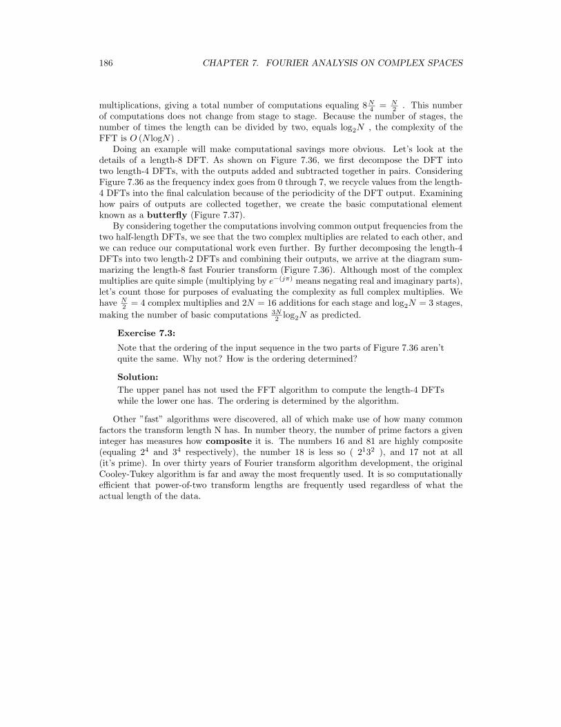
186 CHAPTER 7. FOURIER ANALYSIS ON COMPLEX SPACES
multiplications, giving a total number of computations equaling 8N4 = N
2 . This numberof computations does not change from stage to stage. Because the number of stages, thenumber of times the length can be divided by two, equals log2N , the complexity of theFFT is O (N logN) .
Doing an example will make computational savings more obvious. Let’s look at thedetails of a length-8 DFT. As shown on Figure 7.36, we first decompose the DFT intotwo length-4 DFTs, with the outputs added and subtracted together in pairs. ConsideringFigure 7.36 as the frequency index goes from 0 through 7, we recycle values from the length-4 DFTs into the final calculation because of the periodicity of the DFT output. Examininghow pairs of outputs are collected together, we create the basic computational elementknown as a butterfly (Figure 7.37).
By considering together the computations involving common output frequencies from thetwo half-length DFTs, we see that the two complex multiplies are related to each other, andwe can reduce our computational work even further. By further decomposing the length-4DFTs into two length-2 DFTs and combining their outputs, we arrive at the diagram sum-marizing the length-8 fast Fourier transform (Figure 7.36). Although most of the complexmultiplies are quite simple (multiplying by e−(jπ) means negating real and imaginary parts),let’s count those for purposes of evaluating the complexity as full complex multiplies. Wehave N
2 = 4 complex multiplies and 2N = 16 additions for each stage and log2N = 3 stages,making the number of basic computations 3N
2 log2N as predicted.
Exercise 7.3:
Note that the ordering of the input sequence in the two parts of Figure 7.36 aren’tquite the same. Why not? How is the ordering determined?
Solution:The upper panel has not used the FFT algorithm to compute the length-4 DFTswhile the lower one has. The ordering is determined by the algorithm.
Other ”fast” algorithms were discovered, all of which make use of how many commonfactors the transform length N has. In number theory, the number of prime factors a giveninteger has measures how composite it is. The numbers 16 and 81 are highly composite(equaling 24 and 34 respectively), the number 18 is less so ( 2132 ), and 17 not at all(it’s prime). In over thirty years of Fourier transform algorithm development, the originalCooley-Tukey algorithm is far and away the most frequently used. It is so computationallyefficient that power-of-two transform lengths are frequently used regardless of what theactual length of the data.
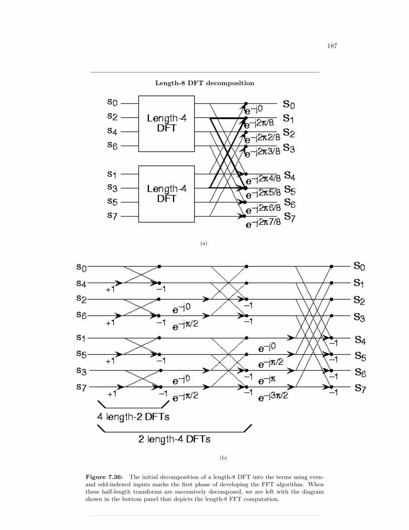
187
Length-8 DFT decomposition
(a)
(b)
Figure 7.36: The initial decomposition of a length-8 DFT into the terms using even-and odd-indexed inputs marks the first phase of developing the FFT algorithm. Whenthese half-length transforms are successively decomposed, we are left with the diagramshown in the bottom panel that depicts the length-8 FFT computation.
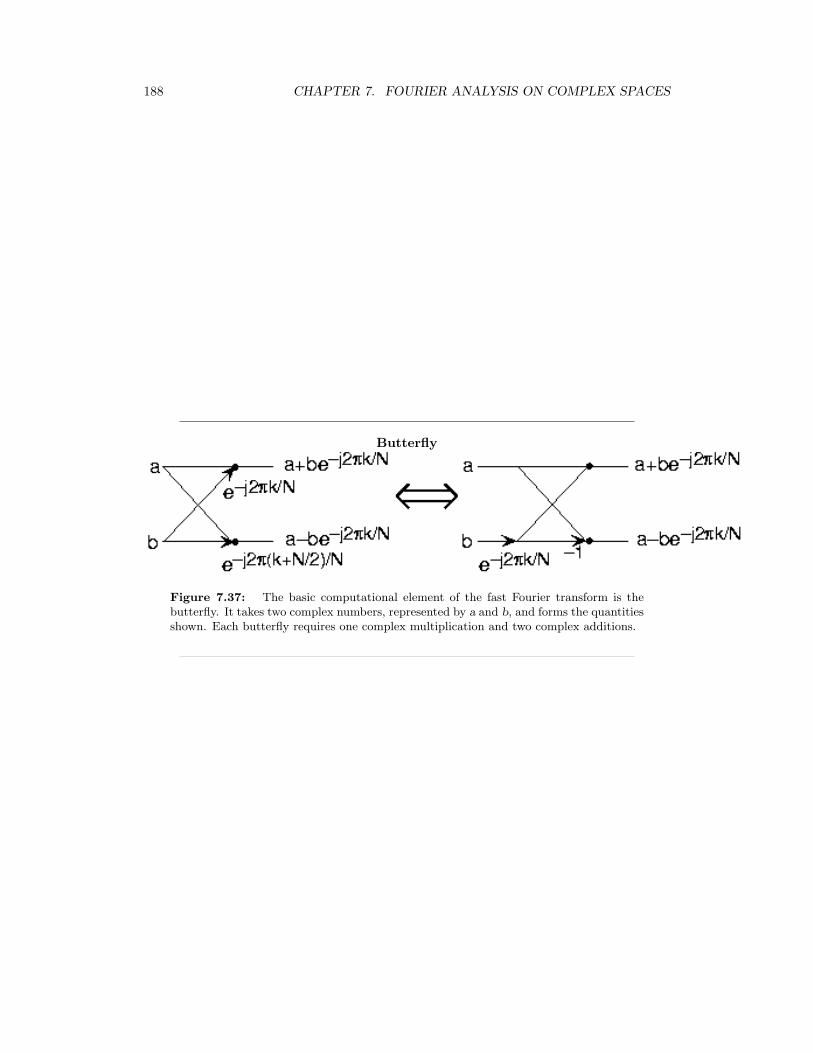
188 CHAPTER 7. FOURIER ANALYSIS ON COMPLEX SPACES
Butterfly
Figure 7.37: The basic computational element of the fast Fourier transform is thebutterfly. It takes two complex numbers, represented by a and b, and forms the quantitiesshown. Each butterfly requires one complex multiplication and two complex additions.
Chapter 8
Convergence
9.1 Convergence of Sequences
8.1.1 What is a Sequence?
sequence : A sequence is a function gn defined on the positive intergers ’n’. Weoften denote a sequence by gn |∞n=1
Example 61:A real number sequence:
gn =1n
Example 62:A vector sequence:
gn =(
sin(
nπ2
)cos(
nπ2
) )
Example 63:A function sequence:
gn (t) =
1 if 0 ≤ t < 1n
0 otherwise
note: A function can be thought of as an infinite dimensionalvector where for each value of ’t’ we have one dimension
8.1.2 Convergence of Real Sequences
limit : A sequence gn |∞n=1 converges to a limit g ∈ R if for every ε > 0 thereis an integer N such that
∀i, i ≥ N : |gi − g| < ε
We usually denote a limit by writing
limi→∞
gi = g
orgi → g
189
190 CHAPTER 8. CONVERGENCE
The above definition means that no matter how small we make ε, except for a finite numberof gi’s, all points of the sequence are within distance ε of g.
Example 8.1:
We are given the following convergent sequence:
gn =1n
(8.1)
Intuitively we can assume the following limit:
limn→∞
gn = 0
Let us prove this rigorously. Say that we are given a real number ε > 0. Let uschoose N = d 1
ε e, where dxe denotes the smallest integer larger than x. Then forn ≥ N we have
|gn − 0| = 1n≤ 1N
< ε
Thus,lim
n→∞gn = 0
Example 8.2:
Now let us look at the following non-convergent sequence
gn =
1 if n = even−1 if n = odd
This sequence oscillates between 1 and -1, so it will therefore never converge.
8.1.2.1 Problems
For practice, say which of the following sequences converge and give their limits if they exist.
1. - gn = n
2. - gn =
1n if n = even−1n if n = odd
3. - gn =
1n if n 6= powerof10
1 otherwise
4. - gn =
n if n < 105
1n if n ≥ 105
5. - gn = sin(
πn
)6. - gn = jn
9.2 Convergence of Vectors
8.2.1 Convergence of Vectors
We now discuss pointwise and norm convergence of vectors. Other types of convergence alsoexist, and one in particular, uniform convergence, can also be studied. For this discussion ,we will assume that the vectors belong to a normed vector space.
191
8.2.1.1 Pointwise Convergence
A sequence gn |∞n=1 converges pointwise to the limit g if each element of gn converges tothe corresponding element in g. Below are few examples to try and help illustrate this idea.
Example 8.3:
gn =(gn [1]gn [2]
)=(
1 + 1n
2− 1n
)First we find the following limits for our two gn’s:
limn→∞
(gn [1]) = 1
limn→∞
(gn [2]) = 2
Therefore we have the following,
limn→∞
gn = g
pointwise, where g =(
12
).
Example 8.4:
∀t, t ∈ R : gn (t) =t
n
As done above, we first want to examine the limit
limn→∞
gn (t0) = limn→∞
t0n
= 0
where t0 ∈ R. Thus limn→∞
gn = g pointwise where g (t) = 0 for all t ∈ R.
8.2.1.2 Norm Convergence
The sequence gn |∞n=1 converges to g in norm if limn→∞
‖ gn − g ‖= 0. Here ‖ @ ‖ is thenorm of the corresponding vector space of gn’s. Intuitively this means the distance betweenvectors gn and g decreases to 0.
Example 8.5:
gn =(
1 + 1n
2− 1n
)Let g =
(12
)‖ gn − g ‖ =
√(1 + 1
n − 1)2 + (−1)2
=√
1n2 + 1
n2
=√
2n
(8.2)
Thus limn→∞
‖ gn − g ‖= 0 Therefore, gn → g in norm.
192 CHAPTER 8. CONVERGENCE
Example 8.6:
gn (t) =
tn if 0 ≤ t ≤ 10 otherwise
Let g (t) = 0 forall t.
‖ gn (t)− g (t) ‖ =∫ 1
0t2
n2 dt
= t3
3n2 |1n=0
= 13n2
(8.3)
Thus limn→∞
‖ gn (t)− g (t) ‖= 0 Therefore, gn (t) → g (t) in norm.
8.2.2 Pointwise vs. Norm Convergence
Theorem 8.1:
For Rm, pointwise and norm convergence are equivalent.
Proof: Pointwise ⇒ Norm
gn [i] → g [i]
Assuming the above, then
(‖ gn − g ‖)2 =m∑
i=1
((gn [i]− g [i])2
)Thus,
limn→∞
(‖ gn − g ‖)2 = limn→∞
∑mi=1 2
=∑m
i=1
(lim
n→∞2)
= 0
(8.4)
Proof: Norm ⇒ Pointwise
‖ gn − g ‖→ 0
limn→∞
∑mi=1 2 =
∑mi=1
(lim
n→∞2)
= 0(8.5)
Since each term is greater than or equal zero, all ’m’ terms must be zero. Thus,
limn→∞
2 = 0
forall i. Therfore,gn → gpointwise
note: In infinite dimensional spaces the above theorem is no longer true. Weprove this with counter examples shown below.
193
8.2.2.1 Counter Examples
Example 8.7: Pointwise @@ Norm
We are given the following function:
gn (t) =n if 0 < t < 1
n0 otherwise
Then limn→∞
gn (t) = 0 This means that,
gn (t) → g (t)
where for all t g (t) = 0.
Now,(‖ gn ‖)2 =
∫∞−∞ (|gn (t) |)2dt
=∫ 1
n
0n2dt
= n→∞(8.6)
Since the function norms blow up, they cannot coverge to any function with finitenorm.
Example 8.8: Norm @@ Pointwise
We are given the following function:
gn (t) =
1 if 0 < t < 1n
0 otherwise if n is even
gn (t) =−1 if 0 < t < 1
n0 otherwise if n is odd
Then,
‖ gn − g ‖=∫ 1
n
0
1dt =1n→ 0
where g (t) = 0 forall t. Therefore,
gn → gin norm
Howerver, at t = 0, gn (t) oscillates between -1 and 1, and so it does not converge.Thus, gn (t) does not converge pointwise.
8.2.2.2 Problems
Prove if the following sequences are pointwise convergent, norm convergent, or both andthen state their limits.
1. - gn (t) =
1nt if 0 < t0 if t ≤ 0
2. - gn (t) =e−(nt) if t ≥ 0
0 if t < 0
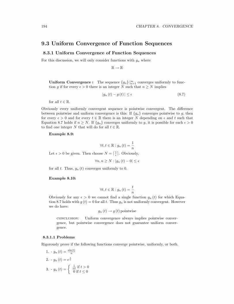
194 CHAPTER 8. CONVERGENCE
9.3 Uniform Convergence of Function Sequences
8.3.1 Uniform Convergence of Function Sequences
For this discussion, we will only consider functions with gn where
R → R
Uniform Convergence : The sequence gn |∞n=1 converges uniformly to func-tion g if for every ε > 0 there is an integer N such that n ≥ N implies
|gn (t)− g (t) | ≤ ε (8.7)
for all t ∈ R.
Obviously every uniformly convergent sequence is pointwise convergent. The differencebetween pointwise and uniform convergence is this: If gn converges pointwise to g, thenfor every ε > 0 and for every t ∈ R there is an integer N depending on ε and t such thatEquation 8.7 holds if n ≥ N . If gn converges uniformly to g, it is possible for each ε > 0to find one integer N that will do for all t ∈ R.
Example 8.9:
∀t, t ∈ R : gn (t) =1n
Let ε > 0 be given. Then choose N = d 1ε e. Obviously,
∀n, n ≥ N : |gn (t)− 0| ≤ ε
for all t. Thus, gn (t) converges uniformly to 0.
Example 8.10:
∀t, t ∈ R : gn (t) =t
n
Obviously for any ε > 0 we cannot find a single function gn (t) for which Equa-tion 8.7 holds with g (t) = 0 for all t. Thus gn is not uniformly convergent. Howeverwe do have:
gn (t) → g (t) pointwise
conclusion: Uniform convergence always implies pointwise conver-gence, but pointwise convergence does not guarantee uniform conver-gence.
8.3.1.1 Problems
Rigorously prove if the following functions converge pointwise, uniformly, or both.
1. - gn (t) = sin(t)n
2. - gn (t) = etn
3. - gn (t) =
1nt if t > 00 if t ≤ 0
Chapter 9
Fourier Transform
10.1 Discrete Fourier Transformation
9.1.1 N-point Discrete Fourier Transform (DFT)
X [k] =N−1∑n=0
(x [n] e(−j) 2π
n kn)∀k, k = 0, . . . , N − 1 (9.1)
x [n] =1N
N−1∑k=0
(X [k] ej 2π
n kn)∀n, n = 0, . . . , N − 1 (9.2)
Note that:
• - X [k] is the DTFT evaluated at ω = 2πN k∀k, k = 0, . . . , N − 1
• - Zero-padding x [n] toM samples prior to the DFT yields anM -point uniform sampledversion of the DTFT:
X(ej 2π
M k)
=N−1∑n=0
(x [n] e(−j) 2π
M k)
(9.3)
X(ej 2π
M k)
=N−1∑n=0
(xzp [n] e(−j) 2π
M k)
X(ej 2π
M k)
= Xzp [k]∀k, k = 0, . . . ,M − 1
• - The N -pt DFT is sufficient to reconstruct the entire DTFT of an N -pt sequence:
X(ejω)
=N−1∑n=0
(x [n] e(−j)ωn
)(9.4)
X(ejω)
=
(N−1∑n=0
(1N
))N−1∑k=0
(X [k] ej 2π
N kne(−j)ωn)
X(ejω)
=
(N−1∑k=0
(X [k])
)1N
N−1∑k=0
(e(−j)(ω− 2π
N k)n)
195
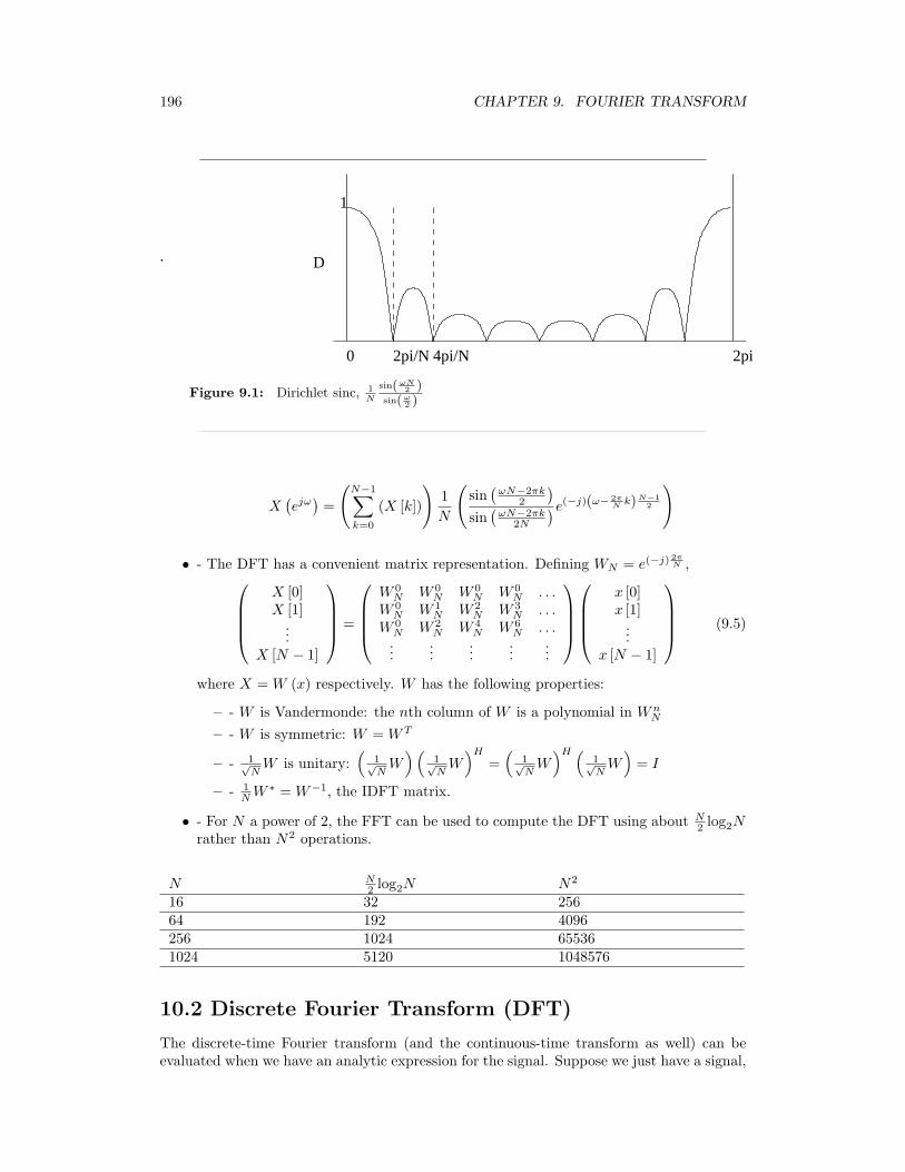
196 CHAPTER 9. FOURIER TRANSFORM
1
0 2pi/N 4pi/N 2pi
D.
Figure 9.1: Dirichlet sinc, 1N
sin( ωN2 )
sin( ω2 )
X(ejω)
=
(N−1∑k=0
(X [k])
)1N
(sin(
ωN−2πk2
)sin(
ωN−2πk2N
)e(−j)(ω− 2πN k)N−1
2
)
• - The DFT has a convenient matrix representation. Defining WN = e(−j) 2πN ,
X [0]X [1]
...X [N − 1]
=
W 0
N W 0N W 0
N W 0N . . .
W 0N W 1
N W 2N W 3
N . . .W 0
N W 2N W 4
N W 6N . . .
......
......
...
x [0]x [1]
...x [N − 1]
(9.5)
where X = W (x) respectively. W has the following properties:
– - W is Vandermonde: the nth column of W is a polynomial in WnN
– - W is symmetric: W = WT
– - 1√NW is unitary:
(1√NW)(
1√NW)H
=(
1√NW)H (
1√NW)
= I
– - 1NW
∗ = W−1, the IDFT matrix.
• - For N a power of 2, the FFT can be used to compute the DFT using about N2 log2N
rather than N2 operations.
N N2 log2N N2
16 32 25664 192 4096256 1024 655361024 5120 1048576
10.2 Discrete Fourier Transform (DFT)
The discrete-time Fourier transform (and the continuous-time transform as well) can beevaluated when we have an analytic expression for the signal. Suppose we just have a signal,
197
such as the speech signal used in the previous chapter, for which there is no formula. Howthen would you compute the spectrum? For example, how did we compute a spectrogramsuch as the one shown in the speech signal example (pg ??)? The Discrete Fourier Transform(DFT) allows the computation of spectra from discrete-time data. While in discrete-timewe can exactly calculate spectra, for analog signals no similar exact spectrum computationexists. For analog-signal spectra, use must build special devices, which turn out in mostcases to consist of A/D converters and discrete-time computations. Certainly discrete-timespectral analysis is more flexible than continuous-time spectral analysis.
The formula for the DTFT (pg ??) is a sum, which conceptually can be easily computedsave for two issues.
• - Signal duration. The sum extends over the signal’s duration, which must be finiteto compute the signal’s spectrum. It is exceedingly difficult to store an infinite-lengthsignal in any case, so we’ll assume that the signal extends over [0, N − 1].
• - Continuous frequency. Subtler than the signal duration issue is the fact that thefrequency variable is continuous: It may only need to span one period, like
[−(
12
), 1
2
]or [0, 1], but the DTFT formula as it stands requires evaluating the spectra at allfrequencies within a period. Let’s compute the spectrum at a few frequencies; themost obvious ones are the equally spaced ones f = k
K , k ∈ k, . . . ,K − 1.
We thus define the discrete Fourier transform (DFT) to be
∀k, k ∈ 0, . . . ,K − 1 : S (k) =N−1∑n=0
(s (n) e−( j2πnk
K ))
(9.6)
Here, S (k) is shorthand for S(ej2π k
K
).
We can compute the spectrum at as many equally spaced frequencies as we like. Notethat you can think about this computationally motivated choice as sampling the spectrum;more about this interpretation later. The issue now is how many frequencies are enough tocapture how the spectrum changes with frequency. One way of answering this question isdetermining an inverse discrete Fourier transform formula: given S (k), k = 0, . . . ,K − 1how do we find s (n), n = 0, . . . , N − 1? Presumably, the formula will be of the forms (n) =
∑K−1k=0
(S (k) e
j2πnkK
). Substituting the DFT formula in this prototype inverse
transform yields
s (n) =K−1∑k=0
(N−1∑m=0
(s (m) e−(j 2πmk
K )ej 2πnkK
))(9.7)
Note that the orthogonality relation we use so often has a different character now.
K−1∑k=0
(e−(j 2πkm
K )ej 2πknK
)=K if m = n, (n±K) , (n± 2K) , . . .
0 otherwise (9.8)
We obtain nonzero value whenever the two indices differ by multiples of K. We can expressthis result as K
∑l (δ (m− n− lK)). Thus, our formula becomes
s (n) =N−1∑m=0
(s (m)K
∞∑l=−∞
(δ (m− n− lK))
)(9.9)
The integers n and m both range over 0, . . . , N − 1. To have an inverse transform, weneed the sum to be a single unit sample for m, n in this range. If it did not, then s (n)
198 CHAPTER 9. FOURIER TRANSFORM
would equal a sum of values, and we would not have a valid transform: Once going into thefrequency domain, we could not get back unambiguously! Clearly, the term l = 0 alwaysprovides a unit sample (we’ll take care of the factor of K soon). If we evaluate the spectrumat fewer frequencies than the signal’s duration, the term corresponding to m = n + Kwill also appear for some values of m, n = 0, . . . , N − 1. This situation means that ourprototype transform equals s (n)+s (n+K) for some values of n. The only way to eliminatethis problem is to require K ≥ N : We must have more frequency samples than the signal’sduration. In this way, we can return from the frequency domain we entered via the DFT.
Exercise 9.1:
When we have fewer frequency samples than the signal’s duration, some discrete-time signal values equal the sum of the original signal values. Given the samplinginterpretation of the spectrum, characterize this effect a different way.
Solution:
This situation amounts to aliasing in the time-domain.
Another way to understand this requirement is to use the theory of linear equations. Ifwe write out the expression for the DFT as a set of linear equations,
s (0) + s (1) + · · ·+ s (N − 1) = S (0) (9.10)
s (0) + s (1) e(−j) 2πK + · · ·+ s (N − 1) e(−j)
2π(N−1)K = S (1)
...
s (0) + s (1) e(−j)2π(K−1)
K + · · ·+ s (N − 1) e(−j)2π(N−1)(K−1)
K = S (K − 1)
we have K equations in N unknowns if we want to find the signal from its sampled spectrum.This requirement is impossible to fulfill if K < N ; we must have K ≥ N . Our orthogonalityrelation essentially says that if we have a sufficient number of equations (frequency samples),the resulting set of equations can indeed be solved.
By convention, the number of DFT frequency values K is chosen to equal the signal’sduration N . The discrete Fourier transform pair consists of
Discrete Fourier Transform Pair
S (k) =N−1∑n=0
(s (n) e−(j 2πnk
N ))
(9.11)
s (n) =1N
N−1∑k=0
(S (k) ej 2πnk
N
)(9.12)
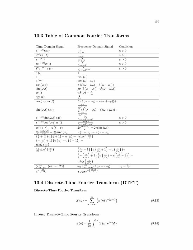
199
10.3 Table of Common Fourier Transforms
Time Domain Signal Frequency Domain Signal Conditione−(at)u (t) 1
a+jω a > 0eatu (−t) 1
a−jω a > 0e−(a|t|) 2a
a2+ω2 a > 0te−(at)u (t) 1
(a+jω)2a > 0
tne−(at)u (t) n!(a+jω)n+1 a > 0
δ (t) 11 2πδ (ω)ejω0t 2πδ (ω − ω0)cos (ω0t) π (δ (ω − ω0) + δ (ω + ω0))sin (ω0t) jπ (δ (ω + ω0)− δ (ω − ω0))u (t) πδ (ω) + 1
jω
sgn (t) 2jω
cos (ω0t)u (t) π2 (δ (ω − ω0) + δ (ω + ω0))+
jωω02−ω2
sin (ω0t)u (t) π2j (δ (ω − ω0)− δ (ω + ω0))+
ω0ω02−ω2
e−(at)sin (ω0t)u (t) ω0(a+jω)2+ω02 a > 0
e−(at)cos (ω0t)u (t) a+jω(a+jω)2+ω02 a > 0
u (t+ τ)− u (t− τ) 2τ sin(ωτ)ωτ = 2τsinc (ωt)
ω0π
sin(ω0t)ω0t = ω0
π sinc (ω0) u (ω + ω0)− u (ω − ω0)(tτ + 1
) (u(
tτ + 1
)− u
(tτ
))+(
−(
tτ
)+ 1) (u(
tτ
)− u
(tτ − 1
))=
triag(
t2τ
) τsinc2(
ωτ2
)ω02π sinc2
(ω0t2
) (ωω0
+ 1)(
u(
ωω0
+ 1)− u
(ωω0
))+(
−(
ωω0
)+ 1)(
u(
ωω0
)− u
(ωω0− 1))
=
triag(
ω2ω0
)∑∞
n=−∞ (δ (t− nT )) ω0
∑∞n=−∞ (δ (ω − nω0)) ω0 = 2π
T
e−(
t2
2σ2
)σ√
2πe−(
σ2ω22
)
10.4 Discrete-Time Fourier Transform (DTFT)
Discrete-Time Fourier Transform
X (ω) =∞∑
n=−∞
(x (n) e−(jωn)
)(9.13)
Inverse Discrete-Time Fourier Transform
x (n) =12π
∫ 2π
0
X (ω) ejωndω (9.14)
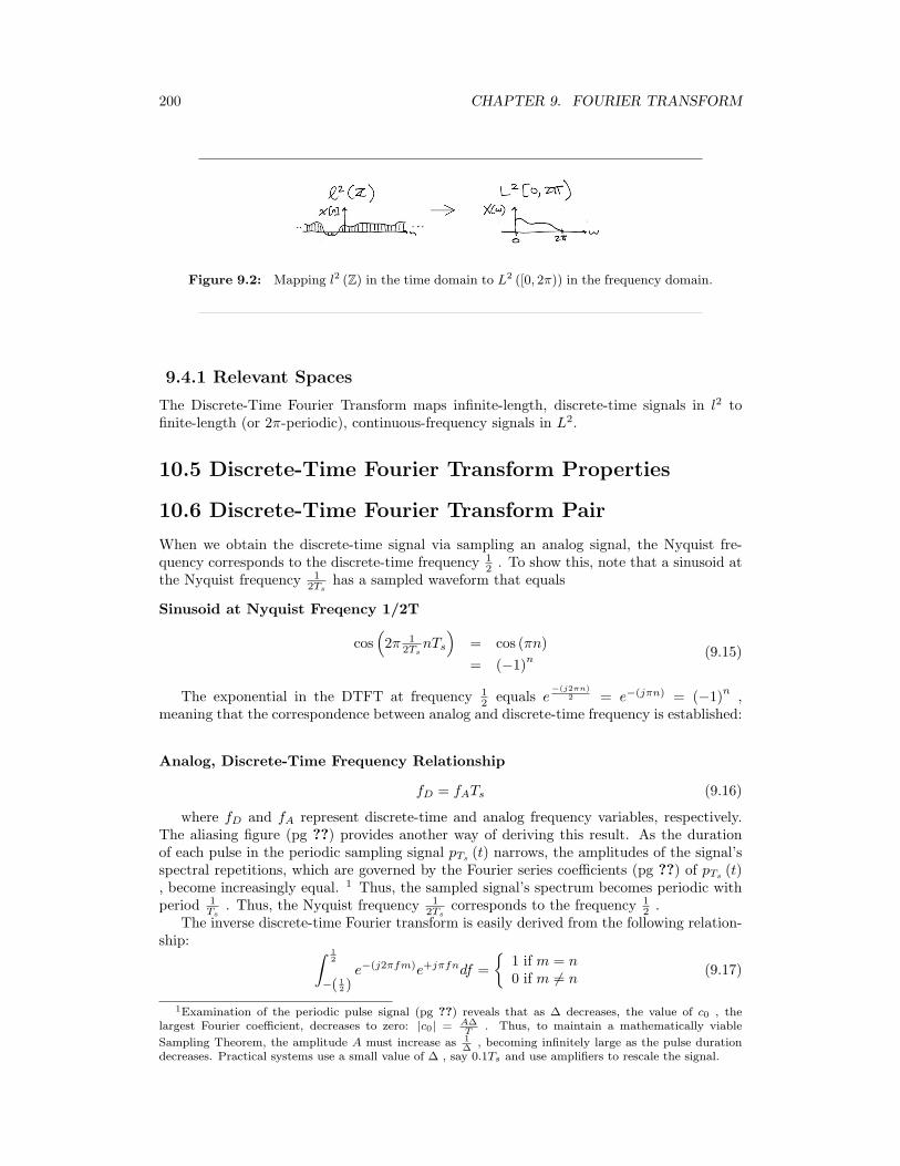
200 CHAPTER 9. FOURIER TRANSFORM
Figure 9.2: Mapping l2 (Z) in the time domain to L2 ([0, 2π)) in the frequency domain.
9.4.1 Relevant Spaces
The Discrete-Time Fourier Transform maps infinite-length, discrete-time signals in l2 tofinite-length (or 2π-periodic), continuous-frequency signals in L2.
10.5 Discrete-Time Fourier Transform Properties
10.6 Discrete-Time Fourier Transform Pair
When we obtain the discrete-time signal via sampling an analog signal, the Nyquist fre-quency corresponds to the discrete-time frequency 1
2 . To show this, note that a sinusoid atthe Nyquist frequency 1
2Tshas a sampled waveform that equals
Sinusoid at Nyquist Freqency 1/2T
cos(2π 1
2TsnTs
)= cos (πn)= (−1)n
(9.15)
The exponential in the DTFT at frequency 12 equals e
−(j2πn)2 = e−(jπn) = (−1)n ,
meaning that the correspondence between analog and discrete-time frequency is established:
Analog, Discrete-Time Frequency Relationship
fD = fATs (9.16)
where fD and fA represent discrete-time and analog frequency variables, respectively.The aliasing figure (pg ??) provides another way of deriving this result. As the durationof each pulse in the periodic sampling signal pTs
(t) narrows, the amplitudes of the signal’sspectral repetitions, which are governed by the Fourier series coefficients (pg ??) of pTs (t), become increasingly equal. 1 Thus, the sampled signal’s spectrum becomes periodic withperiod 1
Ts. Thus, the Nyquist frequency 1
2Tscorresponds to the frequency 1
2 .The inverse discrete-time Fourier transform is easily derived from the following relation-
ship: ∫ 12
−( 12 )e−(j2πfm)e+jπfndf =
1 if m = n0 if m 6= n
(9.17)
1Examination of the periodic pulse signal (pg ??) reveals that as ∆ decreases, the value of c0 , thelargest Fourier coefficient, decreases to zero: |c0| = A∆
T. Thus, to maintain a mathematically viable
Sampling Theorem, the amplitude A must increase as 1∆
, becoming infinitely large as the pulse durationdecreases. Practical systems use a small value of ∆ , say 0.1Ts and use amplifiers to rescale the signal.
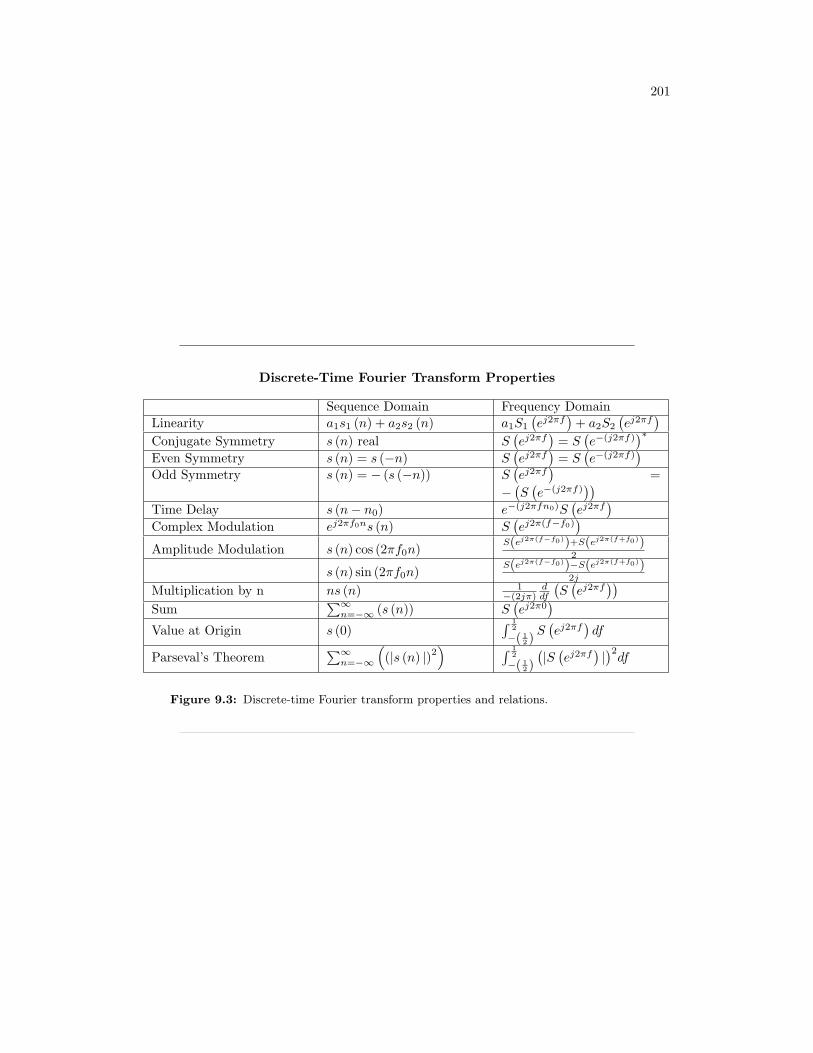
201
Discrete-Time Fourier Transform Properties
Sequence Domain Frequency DomainLinearity a1s1 (n) + a2s2 (n) a1S1
(ej2πf
)+ a2S2
(ej2πf
)Conjugate Symmetry s (n) real S
(ej2πf
)= S
(e−(j2πf)
)∗Even Symmetry s (n) = s (−n) S
(ej2πf
)= S
(e−(j2πf)
)Odd Symmetry s (n) = − (s (−n)) S
(ej2πf
)=
−(S(e−(j2πf)
))Time Delay s (n− n0) e−(j2πfn0)S
(ej2πf
)Complex Modulation ej2πf0ns (n) S
(ej2π(f−f0)
)Amplitude Modulation s (n) cos (2πf0n)
S(ej2π(f−f0))+S(ej2π(f+f0))2
s (n) sin (2πf0n)S(ej2π(f−f0))−S(ej2π(f+f0))
2j
Multiplication by n ns (n) 1−(2jπ)
ddf
(S(ej2πf
))Sum
∑∞n=−∞ (s (n)) S
(ej2π0
)Value at Origin s (0)
∫ 12
−( 12 )S(ej2πf
)df
Parseval’s Theorem∑∞
n=−∞
((|s (n) |)2
) ∫ 12
−( 12 )(|S(ej2πf
)|)2df
Figure 9.3: Discrete-time Fourier transform properties and relations.
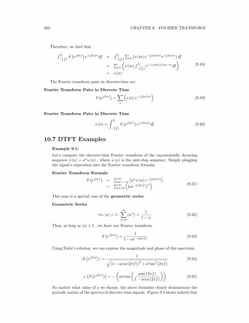
202 CHAPTER 9. FOURIER TRANSFORM
Therefore, we find that∫ 12
−( 12 )S(ej2πf
)e+j2πfndf =
∫ 12
−( 12 )∑
m
(s (m) e−(j2πfm)e+j2πfn
)df
=∑
m
(s (m)
∫ 12
−( 12 )e(−(j2πf))(m−n)df
)= s (n)
(9.18)
The Fourier transform pairs in discrete-time are
Fourier Transform Pairs in Discrete Time
S(ej2πf
)=∑
n
(s (n) e−(j2πfn)
)(9.19)
Fourier Transform Pairs in Discrete Time
s (n) =∫ 1
2
−( 12 )S(ej2πf
)e+j2πfndf (9.20)
10.7 DTFT Examples
Example 9.1:
Let’s compute the discrete-time Fourier transform of the exponentially decayingsequence s (n) = anu (n) , where u (n) is the unit-step sequence. Simply pluggingthe signal’s expression into the Fourier transform formula,
Fourier Transform Formula
S(ej2πf
)=
∑∞n=−∞
(anu (n) e−(j2πfn)
)=
∑∞n=0
((ae−(j2πf)
)n) (9.21)
This sum is a special case of the geometric series .
Geometric Series
∀α, |α| < 1 :∞∑
n=0
(αn) =1
1− α(9.22)
Thus, as long as |a| < 1 , we have our Fourier transform.
S(ej2πf
)=
11− ae−(j2πf)
(9.23)
Using Euler’s relation, we can express the magnitude and phase of this spectrum.
|S(ej2πf
)| = 1√
(1− acos (2πf))2 + a2sin2 (2πf)(9.24)
∠(S(ej2πf
))= −
(arctan
(asin (2πf)
1− acos (2πf)
))(9.25)
No matter what value of a we choose, the above formulae clearly demonstrate theperiodic nature of the spectra of discrete-time signals. Figure 9.4 shows indeed that
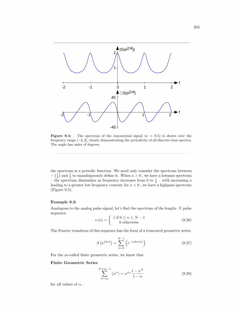
203
-2 -1 0 1 2
1
2
f
|S(ej2πf)|
-2 -1 1 2
-45
45
f
∠S(ej2πf)
Figure 9.4: The spectrum of the exponential signal (a = 0.5) is shown over thefrequency range [−2, 2], clearly demonstrating the periodicity of all discrete-time spectra.The angle has units of degrees.
the spectrum is a periodic function. We need only consider the spectrum between−(
12
)and 1
2 to unambiguously define it. When a > 0 , we have a lowpass spectrum– the spectrum diminishes as frequency increases from 0 to 1
2 – with increasing aleading to a greater low frequency content; for a < 0 , we have a highpass spectrum(Figure 9.5).
Example 9.2:
Analogous to the analog pulse signal, let’s find the spectrum of the length- N pulsesequence.
s (n) =
1 if 0 ≤ n ≤ N − 10 otherwise (9.26)
The Fourier transform of this sequence has the form of a truncated geometric series.
S(ej2πf
)=
N−1∑n=0
(e−(j2πfn)
)(9.27)
For the so-called finite geometric series, we know that
Finite Geometric SeriesN+n0−1∑
n=n0
(αn) = αn01− αN
1− α(9.28)
for all values of α .
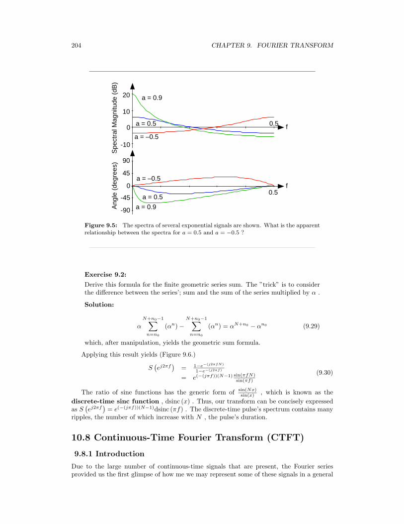
204 CHAPTER 9. FOURIER TRANSFORM
f
a = 0.9
a = 0.5
a = –0.5
Spe
ctra
l Mag
nitu
de (
dB)
-10
0
10
20
0.5
a = 0.9
a = 0.5
a = –0.5
Ang
le (
degr
ees)
f
-90
-45
0
45
90
0.5
Figure 9.5: The spectra of several exponential signals are shown. What is the apparentrelationship between the spectra for a = 0.5 and a = −0.5 ?
Exercise 9.2:
Derive this formula for the finite geometric series sum. The ”trick” is to considerthe difference between the series’; sum and the sum of the series multiplied by α .
Solution:
α
N+n0−1∑n=n0
(αn)−N+n0−1∑
n=n0
(αn) = αN+n0 − αn0 (9.29)
which, after manipulation, yields the geometric sum formula.
Applying this result yields (Figure 9.6.)
S(ej2πf
)= 1−e−(j2πfN)
1−e−(j2πf)
= e(−(jπf))(N−1) sin(πfN)sin(πf)
(9.30)
The ratio of sine functions has the generic form of sin(Nx)sin(x) , which is known as the
discrete-time sinc function , dsinc (x) . Thus, our transform can be concisely expressedas S
(ej2πf
)= e(−(jπf))(N−1)dsinc (πf) . The discrete-time pulse’s spectrum contains many
ripples, the number of which increase with N , the pulse’s duration.
10.8 Continuous-Time Fourier Transform (CTFT)
9.8.1 Introduction
Due to the large number of continuous-time signals that are present, the Fourier seriesprovided us the first glimpse of how me we may represent some of these signals in a general
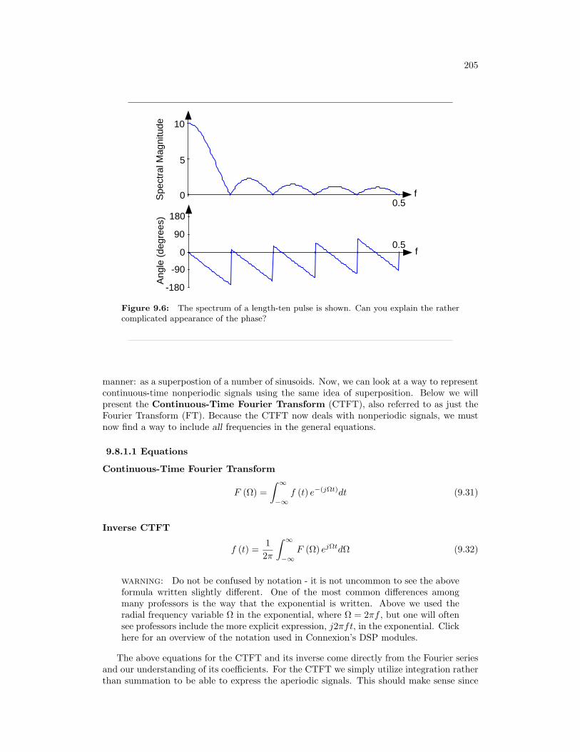
205
f0
5
10
Spe
ctra
l Mag
nitu
de
0.5
-180
-90
0
90
180
f0.5
Ang
le (
degr
ees)
Figure 9.6: The spectrum of a length-ten pulse is shown. Can you explain the rathercomplicated appearance of the phase?
manner: as a superpostion of a number of sinusoids. Now, we can look at a way to representcontinuous-time nonperiodic signals using the same idea of superposition. Below we willpresent the Continuous-Time Fourier Transform (CTFT), also referred to as just theFourier Transform (FT). Because the CTFT now deals with nonperiodic signals, we mustnow find a way to include all frequencies in the general equations.
9.8.1.1 Equations
Continuous-Time Fourier Transform
F (Ω) =∫ ∞
−∞f (t) e−(jΩt)dt (9.31)
Inverse CTFT
f (t) =12π
∫ ∞
−∞F (Ω) ejΩtdΩ (9.32)
warning: Do not be confused by notation - it is not uncommon to see the aboveformula written slightly different. One of the most common differences amongmany professors is the way that the exponential is written. Above we used theradial frequency variable Ω in the exponential, where Ω = 2πf , but one will oftensee professors include the more explicit expression, j2πft, in the exponential. Clickhere for an overview of the notation used in Connexion’s DSP modules.
The above equations for the CTFT and its inverse come directly from the Fourier seriesand our understanding of its coefficients. For the CTFT we simply utilize integration ratherthan summation to be able to express the aperiodic signals. This should make sense since
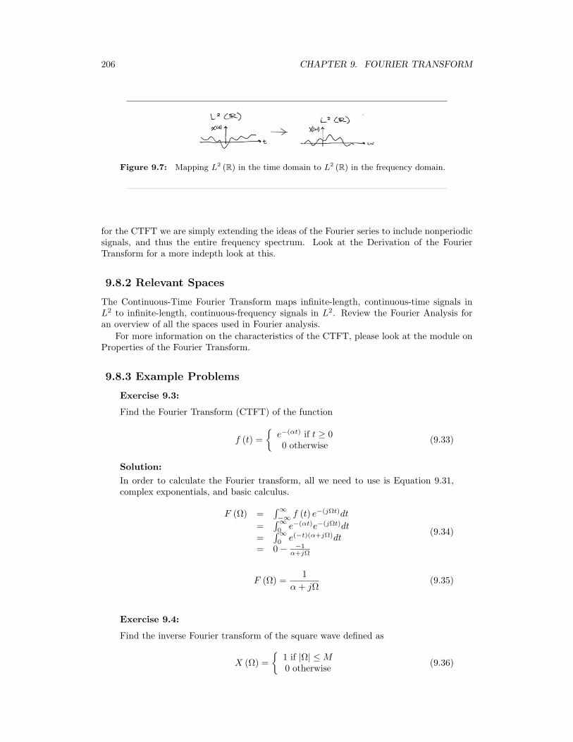
206 CHAPTER 9. FOURIER TRANSFORM
Figure 9.7: Mapping L2 (R) in the time domain to L2 (R) in the frequency domain.
for the CTFT we are simply extending the ideas of the Fourier series to include nonperiodicsignals, and thus the entire frequency spectrum. Look at the Derivation of the FourierTransform for a more indepth look at this.
9.8.2 Relevant Spaces
The Continuous-Time Fourier Transform maps infinite-length, continuous-time signals inL2 to infinite-length, continuous-frequency signals in L2. Review the Fourier Analysis foran overview of all the spaces used in Fourier analysis.
For more information on the characteristics of the CTFT, please look at the module onProperties of the Fourier Transform.
9.8.3 Example Problems
Exercise 9.3:
Find the Fourier Transform (CTFT) of the function
f (t) =e−(αt) if t ≥ 00 otherwise
(9.33)
Solution:In order to calculate the Fourier transform, all we need to use is Equation 9.31,complex exponentials, and basic calculus.
F (Ω) =∫∞−∞ f (t) e−(jΩt)dt
=∫∞0e−(αt)e−(jΩt)dt
=∫∞0e(−t)(α+jΩ)dt
= 0− −1α+jΩ
(9.34)
F (Ω) =1
α+ jΩ(9.35)
Exercise 9.4:
Find the inverse Fourier transform of the square wave defined as
X (Ω) =
1 if |Ω| ≤M0 otherwise (9.36)
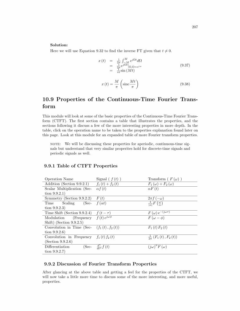
207
Solution:Here we will use Equation 9.32 to find the inverse FT given that t 6= 0.
x (t) = 12π
∫M
−MejΩtdΩ
= 12π e
jΩt|Ω,Ω=ejw
= 1πt sin (Mt)
(9.37)
x (t) =M
π
(sinc
Mt
π
)(9.38)
10.9 Properties of the Continuous-Time Fourier Trans-form
This module will look at some of the basic properties of the Continuous-Time Fourier Trans-form (CTFT). The first section contains a table that illustrates the properties, and thesections following it discuss a few of the more interesting properties in more depth. In thetable, click on the operation name to be taken to the properties explanation found later onthis page. Look at this module for an expanded table of more Fourier transform properties.
note: We will be discussing these properties for aperiodic, continuous-time sig-nals but understand that very similar properites hold for discrete-time signals andperiodic signals as well.
9.9.1 Table of CTFT Properties
Operation Name Signal ( f (t) ) Transform ( F (ω) )Addition (Section 9.9.2.1) f1 (t) + f2 (t) F1 (ω) + F2 (ω)Scalar Multiplication (Sec-tion 9.9.2.1)
αf (t) αF (t)
Symmetry (Section 9.9.2.2) F (t) 2πf (−ω)Time Scaling (Sec-tion 9.9.2.3)
f (αt) 1|α|F
(ωα
)Time Shift (Section 9.9.2.4) f (t− τ) F (ω) e−(jωτ)
Modulation (FrequencyShift) (Section 9.9.2.5)
f (t) ejωφ F (ω − φ)
Convolution in Time (Sec-tion 9.9.2.6)
(f1 (t) , f2 (t)) F1 (t)F2 (t)
Convolution in Frequency(Section 9.9.2.6)
f1 (t) f2 (t) 12π (F1 (t) , F2 (t))
Differentiation (Sec-tion 9.9.2.7)
dn
dtn f (t) (jω)nF (ω)
9.9.2 Discussion of Fourier Transform Properties
After glancing at the above table and getting a feel for the properties of the CTFT, wewill now take a little more time to discuss some of the more interesting, and more useful,properties.
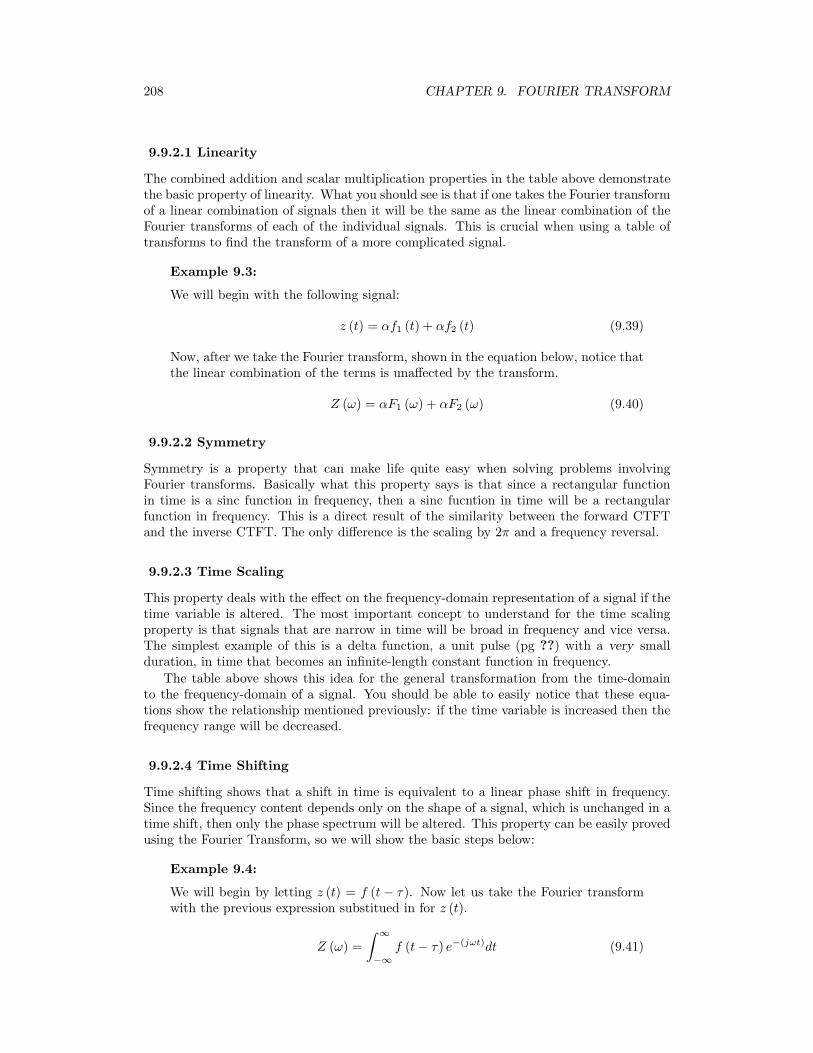
208 CHAPTER 9. FOURIER TRANSFORM
9.9.2.1 Linearity
The combined addition and scalar multiplication properties in the table above demonstratethe basic property of linearity. What you should see is that if one takes the Fourier transformof a linear combination of signals then it will be the same as the linear combination of theFourier transforms of each of the individual signals. This is crucial when using a table oftransforms to find the transform of a more complicated signal.
Example 9.3:
We will begin with the following signal:
z (t) = αf1 (t) + αf2 (t) (9.39)
Now, after we take the Fourier transform, shown in the equation below, notice thatthe linear combination of the terms is unaffected by the transform.
Z (ω) = αF1 (ω) + αF2 (ω) (9.40)
9.9.2.2 Symmetry
Symmetry is a property that can make life quite easy when solving problems involvingFourier transforms. Basically what this property says is that since a rectangular functionin time is a sinc function in frequency, then a sinc fucntion in time will be a rectangularfunction in frequency. This is a direct result of the similarity between the forward CTFTand the inverse CTFT. The only difference is the scaling by 2π and a frequency reversal.
9.9.2.3 Time Scaling
This property deals with the effect on the frequency-domain representation of a signal if thetime variable is altered. The most important concept to understand for the time scalingproperty is that signals that are narrow in time will be broad in frequency and vice versa.The simplest example of this is a delta function, a unit pulse (pg ??) with a very smallduration, in time that becomes an infinite-length constant function in frequency.
The table above shows this idea for the general transformation from the time-domainto the frequency-domain of a signal. You should be able to easily notice that these equa-tions show the relationship mentioned previously: if the time variable is increased then thefrequency range will be decreased.
9.9.2.4 Time Shifting
Time shifting shows that a shift in time is equivalent to a linear phase shift in frequency.Since the frequency content depends only on the shape of a signal, which is unchanged in atime shift, then only the phase spectrum will be altered. This property can be easily provedusing the Fourier Transform, so we will show the basic steps below:
Example 9.4:
We will begin by letting z (t) = f (t− τ). Now let us take the Fourier transformwith the previous expression substitued in for z (t).
Z (ω) =∫ ∞
−∞f (t− τ) e−(jωt)dt (9.41)
209
Now let us make a simple change of variables, where σ = t − τ . Through thecalculations below, you can see that only the variable in the exponential are alteredthus only changing the phase in the frequency domain.
Z (ω) =∫∞−∞ f (σ) e−(jω(σ+τ)t)dτ
= e−(jωτ)∫∞−∞ f (σ) e−(jωσ)dσ
= e−(jωτ)F (ω)(9.42)
9.9.2.5 Modulation (Frequency Shift)
Modulation is absolutely imperative to communications applications. Being able to shift asignal to a different frequency, allows us to take advantage of different parts of the electro-magnetic spectrum is what allows us to transmit television, radio and other applicationsthrough the same space without significant interference.
The proof of the frequency shift property is very similar to that of the time shift (Sec-tion 9.9.2.4); however, here we would use the inverse Fourier transform in place of the Fouriertransform. Since we went through the steps in the previous, time-shift proof, below we willjust show the initial and final step to this proof:
z (t) =12π
∫ ∞
−∞F (ω − φ) ejωtdω (9.43)
Now we would simply reduce this equation through another change of variables and simplifythe terms. Then we will prove the property experssed in the table above:
z (t) = f (t) ejφt (9.44)
9.9.2.6 Convolution
Convolution is one of the big reasons for converting signals to the frequency domain, sinceconvolution in time becomes multiplication in frequency. This property is also anotherexcellent example of symmetry between time and frequency. It also shows that there maybe little to gain by changing to the frequency domain when multiplication in time is involved.
We will introduce the convolution integral here, but if you have not seen this before orneed to refresh your memory, then look at the continuous-time convolution module for amore in depth explanation and derivation.
y (t) = (f1 (t) , f2 (t))=
∫∞−∞ f1 (τ) f2 (t− τ) dτ (9.45)
9.9.2.7 Time Differentiation
Since LTI systems can be represented in terms of differential equations, it is apparent withthis property that converting to the frequency domain may allow us to convert these com-plicated differential equations to simpler equations involving multiplication and addition.This is often looked at in more detail during the study of the Laplace Transform.

210 CHAPTER 9. FOURIER TRANSFORM
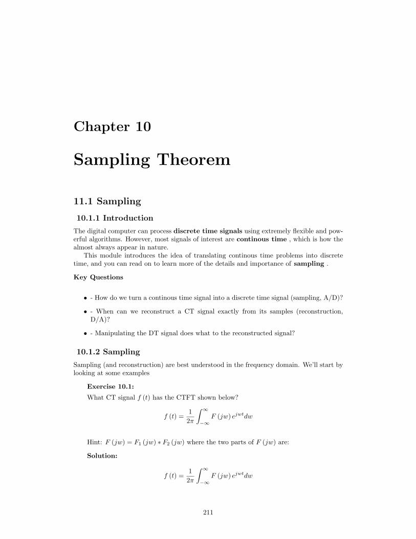
Chapter 10
Sampling Theorem
11.1 Sampling
10.1.1 Introduction
The digital computer can process discrete time signals using extremely flexible and pow-erful algorithms. However, most signals of interest are continous time , which is how thealmost always appear in nature.
This module introduces the idea of translating continous time problems into discretetime, and you can read on to learn more of the details and importance of sampling .
Key Questions
• - How do we turn a continous time signal into a discrete time signal (sampling, A/D)?
• - When can we reconstruct a CT signal exactly from its samples (reconstruction,D/A)?
• - Manipulating the DT signal does what to the reconstructed signal?
10.1.2 Sampling
Sampling (and reconstruction) are best understood in the frequency domain. We’ll start bylooking at some examples
Exercise 10.1:
What CT signal f (t) has the CTFT shown below?
f (t) =12π
∫ ∞
−∞F (jw) ejwtdw
Hint: F (jw) = F1 (jw) ∗ F2 (jw) where the two parts of F (jw) are:
Solution:
f (t) =12π
∫ ∞
−∞F (jw) ejwtdw
211
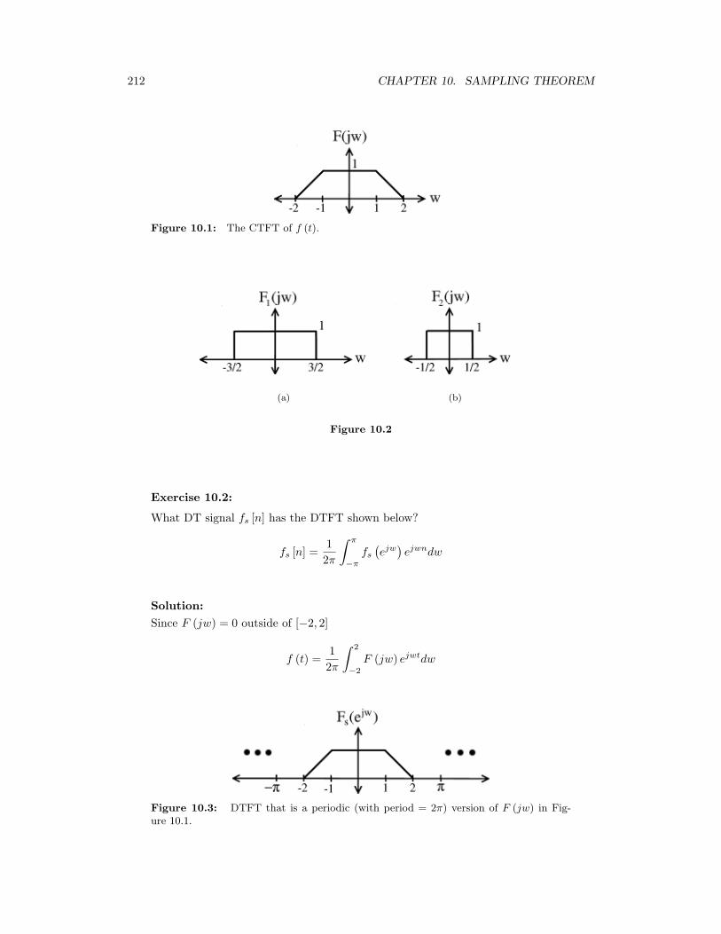
212 CHAPTER 10. SAMPLING THEOREM
Figure 10.1: The CTFT of f (t).
(a) (b)
Figure 10.2
Exercise 10.2:
What DT signal fs [n] has the DTFT shown below?
fs [n] =12π
∫ π
−π
fs
(ejw)ejwndw
Solution:Since F (jw) = 0 outside of [−2, 2]
f (t) =12π
∫ 2
−2
F (jw) ejwtdw
Figure 10.3: DTFT that is a periodic (with period = 2π) version of F (jw) in Fig-ure 10.1.
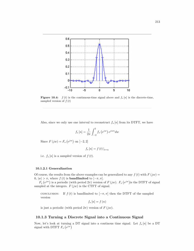
213
Figure 10.4: f (t) is the continuous-time signal above and fs [n] is the discrete-time,sampled version of f (t)
Also, since we only use one interval to reconstruct fs [n] from its DTFT, we have
fs [n] =12π
∫ 2
−2
fs
(ejw)ejwndw
Since F (jw) = Fs
(ejw)
on [−2, 2]
fs [n] = f (t) |t=n
i.e. fs [n] is a sampled version of f (t).
10.1.2.1 Generalization
Of course, the results from the above examples can be generalized to any f (t) with F (jw) =0, |w| > π, where f (t) is bandlimited to [−π, π].
Fs
(ejw)
is a periodic (with period 2π) version of F (jw). Fs
(ejw)is the DTFT of signal
sampled at the integers. F (jw) is the CTFT of signal.
conclusion: If f (t) is bandlimited to [−π, π] then the DTFT of the sampledversion
fs [n] = f (n)
is just a periodic (with period 2π) version of F (jw).
10.1.3 Turning a Discrete Signal into a Continuous Signal
Now, let’s look at turning a DT signal into a continous time signal. Let fs [n] be a DTsignal with DTFT Fs
(ejw)
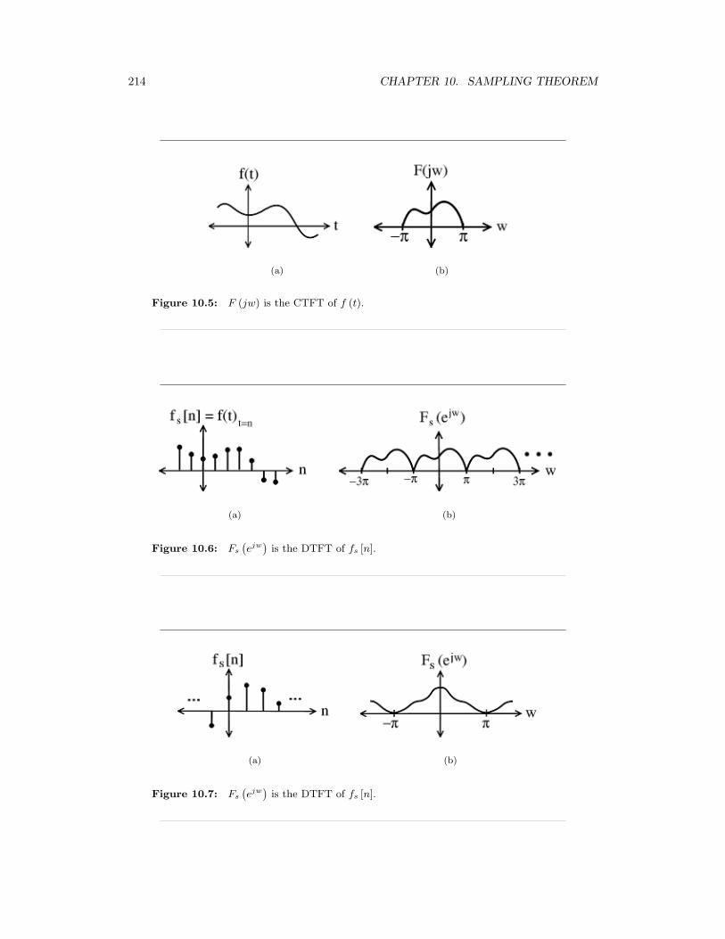
214 CHAPTER 10. SAMPLING THEOREM
(a) (b)
Figure 10.5: F (jw) is the CTFT of f (t).
(a) (b)
Figure 10.6: Fs
(ejw
)is the DTFT of fs [n].
(a) (b)
Figure 10.7: Fs
(ejw
)is the DTFT of fs [n].
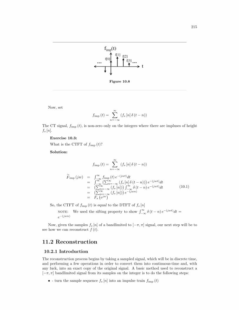
215
Figure 10.8
Now, set
fimp (t) =∞∑
n=−∞(fs [n] δ (t− n))
The CT signal, fimp (t), is non-zero only on the integers where there are impluses of heightfs [n].
Exercise 10.3:
What is the CTFT of fimp (t)?
Solution:
fimp (t) =∞∑
n=−∞(fs [n] δ (t− n))
∼F imp (jw) =
∫∞−∞ fimp (t) e−(jwt)dt
=∫∞−∞
(∑∞n=−∞ (fs [n] δ (t− n))
)e−(jwt)dt
=(∑∞
n=−∞ (fs [n])) ∫∞
−∞ δ (t− n) e−(jwt)dt
=(∑∞
n=−∞ (fs [n]))e−(jwn)
= Fs
(ejw)
(10.1)
So, the CTFT of fimp (t) is equal to the DTFT of fs [n]
note: We used the sifting property to show∫∞−∞ δ (t− n) e−(jwt)dt =
e−(jwn)
Now, given the samples fs [n] of a bandlimited to [−π, π] signal, our next step will be tosee how we can reconstruct f (t).
11.2 Reconstruction
10.2.1 Introduction
The reconstruction process begins by taking a sampled signal, which will be in discrete time,and performing a few operations in order to convert them into continuous-time and, withany luck, into an exact copy of the original signal. A basic method used to reconstruct a[−π, π] bandlimited signal from its samples on the integer is to do the following steps:
• - turn the sample sequence fs [n] into an impulse train fimp (t)
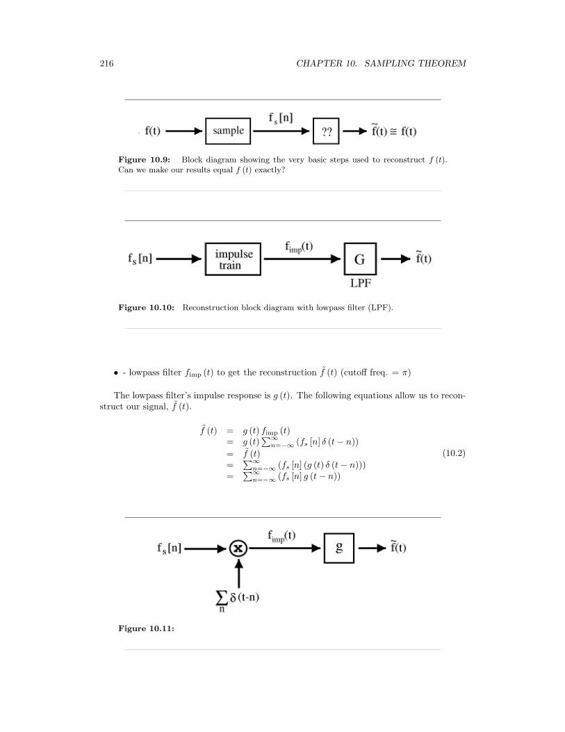
216 CHAPTER 10. SAMPLING THEOREM
Figure 10.9: Block diagram showing the very basic steps used to reconstruct f (t).Can we make our results equal f (t) exactly?
Figure 10.10: Reconstruction block diagram with lowpass filter (LPF).
• - lowpass filter fimp (t) to get the reconstruction f (t) (cutoff freq. = π)
The lowpass filter’s impulse response is g (t). The following equations allow us to recon-struct our signal, f (t).
f (t) = g (t) fimp (t)= g (t)
∑∞n=−∞ (fs [n] δ (t− n))
= f (t)=
∑∞n=−∞ (fs [n] (g (t) δ (t− n)))
=∑∞
n=−∞ (fs [n] g (t− n))
(10.2)
Figure 10.11:
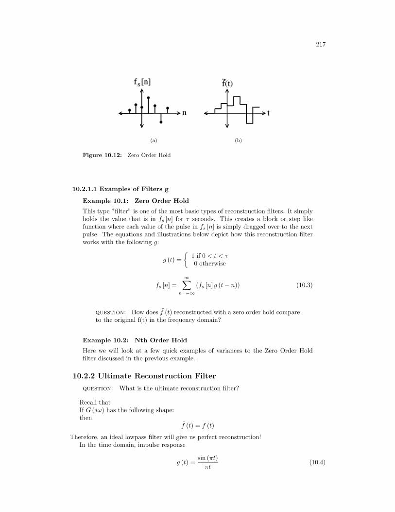
217
(a) (b)
Figure 10.12: Zero Order Hold
10.2.1.1 Examples of Filters g
Example 10.1: Zero Order Hold
This type ”filter” is one of the most basic types of reconstruction filters. It simplyholds the value that is in fs [n] for τ seconds. This creates a block or step likefunction where each value of the pulse in fs [n] is simply dragged over to the nextpulse. The equations and illustrations below depict how this reconstruction filterworks with the following g:
g (t) =
1 if 0 < t < τ0 otherwise
fs [n] =∞∑
n=−∞(fs [n] g (t− n)) (10.3)
question: How does f (t) reconstructed with a zero order hold compareto the original f(t) in the frequency domain?
Example 10.2: Nth Order Hold
Here we will look at a few quick examples of variances to the Zero Order Holdfilter discussed in the previous example.
10.2.2 Ultimate Reconstruction Filter
question: What is the ultimate reconstruction filter?
Recall thatIf G (jω) has the following shape:then
f (t) = f (t)
Therefore, an ideal lowpass filter will give us perfect reconstruction!In the time domain, impulse response
g (t) =sin (πt)πt
(10.4)
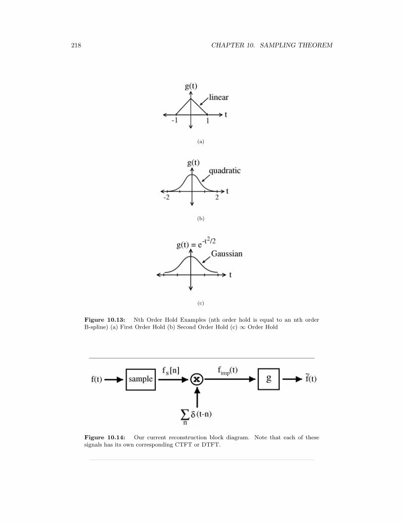
218 CHAPTER 10. SAMPLING THEOREM
(a)
(b)
(c)
Figure 10.13: Nth Order Hold Examples (nth order hold is equal to an nth orderB-spline) (a) First Order Hold (b) Second Order Hold (c) ∞ Order Hold
Figure 10.14: Our current reconstruction block diagram. Note that each of thesesignals has its own corresponding CTFT or DTFT.
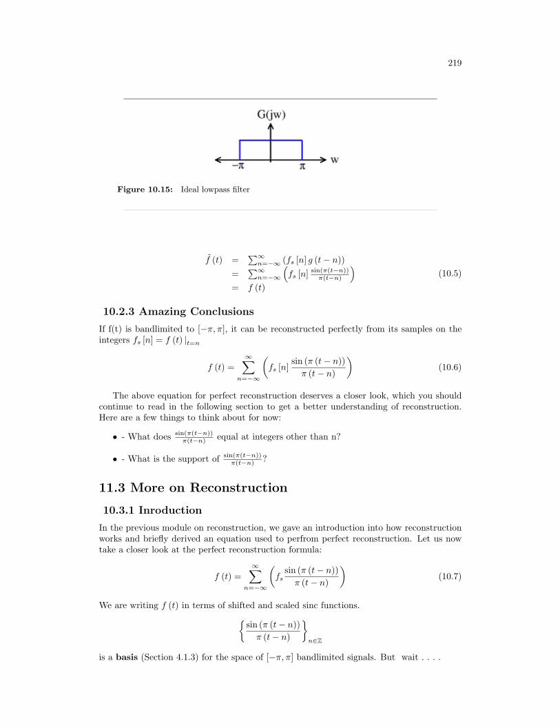
219
Figure 10.15: Ideal lowpass filter
f (t) =∑∞
n=−∞ (fs [n] g (t− n))
=∑∞
n=−∞
(fs [n] sin(π(t−n))
π(t−n)
)= f (t)
(10.5)
10.2.3 Amazing Conclusions
If f(t) is bandlimited to [−π, π], it can be reconstructed perfectly from its samples on theintegers fs [n] = f (t) |t=n
f (t) =∞∑
n=−∞
(fs [n]
sin (π (t− n))π (t− n)
)(10.6)
The above equation for perfect reconstruction deserves a closer look, which you shouldcontinue to read in the following section to get a better understanding of reconstruction.Here are a few things to think about for now:
• - What does sin(π(t−n))π(t−n) equal at integers other than n?
• - What is the support of sin(π(t−n))π(t−n) ?
11.3 More on Reconstruction
10.3.1 Inroduction
In the previous module on reconstruction, we gave an introduction into how reconstructionworks and briefly derived an equation used to perfrom perfect reconstruction. Let us nowtake a closer look at the perfect reconstruction formula:
f (t) =∞∑
n=−∞
(fs
sin (π (t− n))π (t− n)
)(10.7)
We are writing f (t) in terms of shifted and scaled sinc functions.sin (π (t− n))π (t− n)
n∈Z
is a basis (Section 4.1.3) for the space of [−π, π] bandlimited signals. But wait . . . .
220 CHAPTER 10. SAMPLING THEOREM
10.3.1.1 Derive Reconstruction Formulas
What issin (π (t− n))π (t− n)
· sin (π (t− k))π (t− k)
=? (10.8)
This inner product can be hard to calculate in the time domain, so let’s use PlancharelTheorem
· · · = 12π
∫ π
−π
e−(jωn)ejωkdω (10.9)
if n = ksincn · sinck = 1
2π
∫ π
−πe−(jωn)ejωkdω
= 1(10.10)
if n 6= k
sincn · sinck = 12π
∫ π
−πe−(jωn)ejωndω
= 12π
∫ π
−πejω(k−n)dω
= 12π
sin(π(k−n))j(k−n)
= 0
(10.11)
note: In Equation 10.11 we used the fact that the integral of sinusoid over acomplete interval is 0 to simplify our equation.
So,sin (π (t− n))π (t− n)
· sin (π (t− k))π (t− k)
=
1 if n = k0 if n 6= k
(10.12)
Therefore sin (π (t− n))π (t− n)
n∈Z
is an orthonormal basis (Section 6.7.3) (ONB) for the space of [−π, π] bandlimited functions.
sampling: Sampling is the same as calculating ONB coefficients, which is innerproducts with sincs
10.3.1.2 Summary
One last time for f (t) [−π, π] bandlimited
Synthesis
f (t) =∞∑
n=−∞
(fs [n]
sin (π (t− n))π (t− n)
)(10.13)
Analysis
fs [n] = f (t) |t=n (10.14)
In order to understand a little more about how we can reconstruct a signal exactly, it willbe useful to examine the relationships between the fourier transforms (CTFT and DTFT)in more depth.
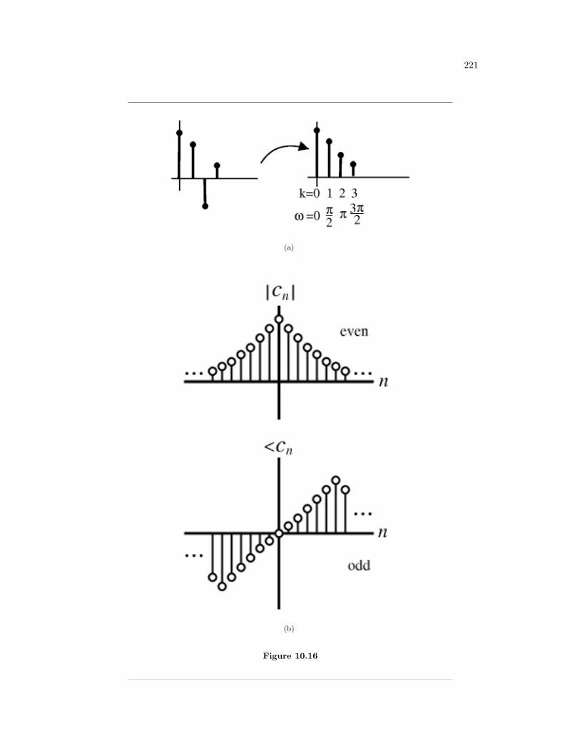
221
(a)
(b)
Figure 10.16
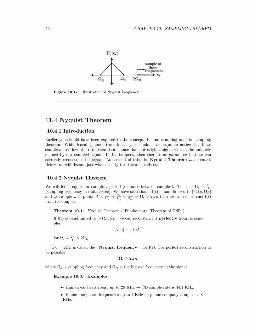
222 CHAPTER 10. SAMPLING THEOREM
Figure 10.17: Illustration of Nyquist Frequency
11.4 Nyquist Theorem
10.4.1 Introduction
Earlier you should have been exposed to the concepts behind sampling and the samplingtheorem. While learning about these ideas, you should have begun to notice that if wesample at too low of a rate, there is a chance that our original signal will not be uniquelydefined by our sampled signal. If this happens, then there is no garauntee that we cancorrectly reconstruct the signal. As a result of this, the Nyquist Theorem was created.Below, we will discuss just what exactly this theorem tells us.
10.4.2 Nyquist Theorem
We will let T equal our sampling period (distance between samples). Then let Ωs = 2πT
(sampling frequency in radians/sec). We have seen that if f(t) is bandlimited to [−ΩB ,ΩB ]and we sample with period T < π
Ωb⇒ 2π
Ωs< π
ΩB⇒ Ωs > 2ΩB then we can reconstruct f(t)
from its samples.
Theorem 10.1: Nyquist Theorem (”Fundamental Theorem of DSP”)
If f(t) is bandlimited to [−ΩB ,ΩB ], we can reconstruct it perfectly from its sam-ples
fs [n] = f (nT )
for Ωs = 2πT > 2ΩB
ΩN = 2ΩB is called the ”Nyquist frequency ” for f(t). For perfect reconstruction tobe possible
Ωs ≥ 2ΩB
where Ωs is sampling frequency and ΩB is the highest frequency in the signal.
Example 10.3: Examples:
•- Human ear hears freqs. up to 20 KHz → CD sample rate is 44.1 KHz.
•- Phone line passes frequencies up to 4 KHz → phone company samples at 8KHz.
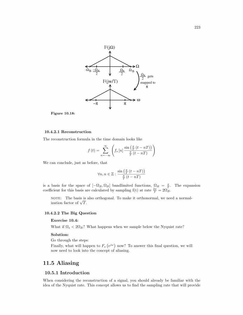
223
Figure 10.18:
10.4.2.1 Reconstruction
The reconstruction formula in the time domain looks like
f (t) =∞∑
n=−∞
(fs [n]
sin(
πT (t− nT )
)πT (t− nT )
)
We can conclude, just as before, that
∀n, n ∈ Z :sin(
πT (t− nT )
)πT (t− nT )
is a basis for the space of [−ΩB ,ΩB ] bandlimited functions, ΩB = πT . The expansion
coefficient for this basis are calculated by sampling f(t) at rate 2πT = 2ΩB .
note: The basis is also orthogonal. To make it orthonormal, we need a normal-ization factor of
√T .
10.4.2.2 The Big Question
Exercise 10.4:
What if Ωs < 2ΩB? What happens when we sample below the Nyquist rate?
Solution:Go through the steps:Finally, what will happen to Fs
(ejω)
now? To answer this final question, we willnow need to look into the concept of aliasing.
11.5 Aliasing
10.5.1 Introduction
When considering the reconstruction of a signal, you should already be familiar with theidea of the Nyquist rate. This concept allows us to find the sampling rate that will provide
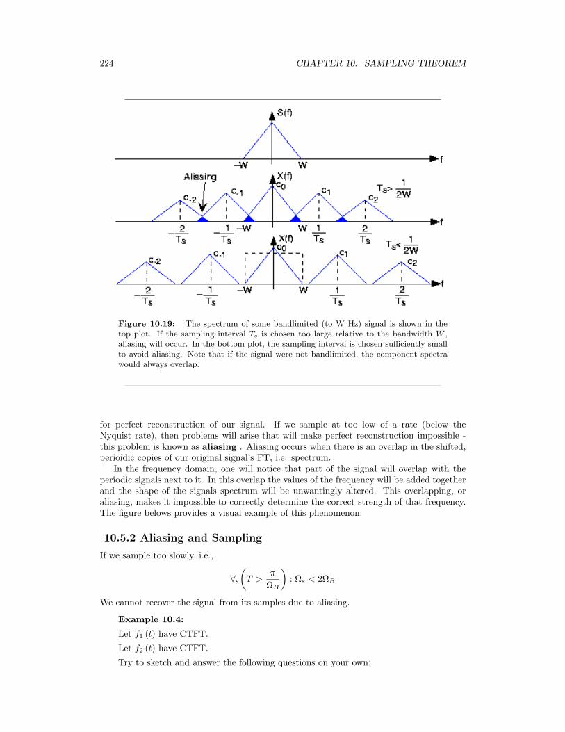
224 CHAPTER 10. SAMPLING THEOREM
Figure 10.19: The spectrum of some bandlimited (to W Hz) signal is shown in thetop plot. If the sampling interval Ts is chosen too large relative to the bandwidth W ,aliasing will occur. In the bottom plot, the sampling interval is chosen sufficiently smallto avoid aliasing. Note that if the signal were not bandlimited, the component spectrawould always overlap.
for perfect reconstruction of our signal. If we sample at too low of a rate (below theNyquist rate), then problems will arise that will make perfect reconstruction impossible -this problem is known as aliasing . Aliasing occurs when there is an overlap in the shifted,perioidic copies of our original signal’s FT, i.e. spectrum.
In the frequency domain, one will notice that part of the signal will overlap with theperiodic signals next to it. In this overlap the values of the frequency will be added togetherand the shape of the signals spectrum will be unwantingly altered. This overlapping, oraliasing, makes it impossible to correctly determine the correct strength of that frequency.The figure belows provides a visual example of this phenomenon:
10.5.2 Aliasing and Sampling
If we sample too slowly, i.e.,
∀,(T >
π
ΩB
): Ωs < 2ΩB
We cannot recover the signal from its samples due to aliasing.
Example 10.4:
Let f1 (t) have CTFT.
Let f2 (t) have CTFT.
Try to sketch and answer the following questions on your own:
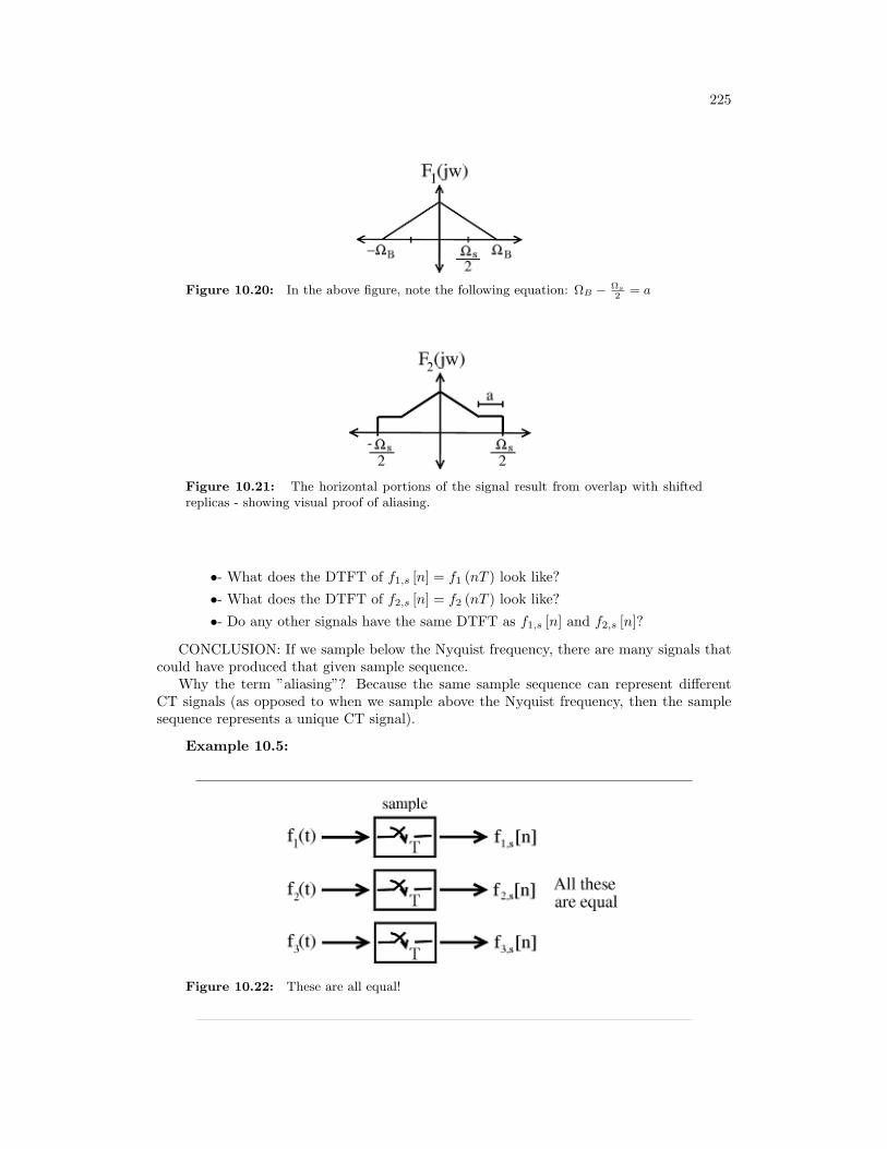
225
Figure 10.20: In the above figure, note the following equation: ΩB − Ωs2
= a
Figure 10.21: The horizontal portions of the signal result from overlap with shiftedreplicas - showing visual proof of aliasing.
•- What does the DTFT of f1,s [n] = f1 (nT ) look like?
•- What does the DTFT of f2,s [n] = f2 (nT ) look like?
•- Do any other signals have the same DTFT as f1,s [n] and f2,s [n]?
CONCLUSION: If we sample below the Nyquist frequency, there are many signals thatcould have produced that given sample sequence.
Why the term ”aliasing”? Because the same sample sequence can represent differentCT signals (as opposed to when we sample above the Nyquist frequency, then the samplesequence represents a unique CT signal).
Example 10.5:
Figure 10.22: These are all equal!
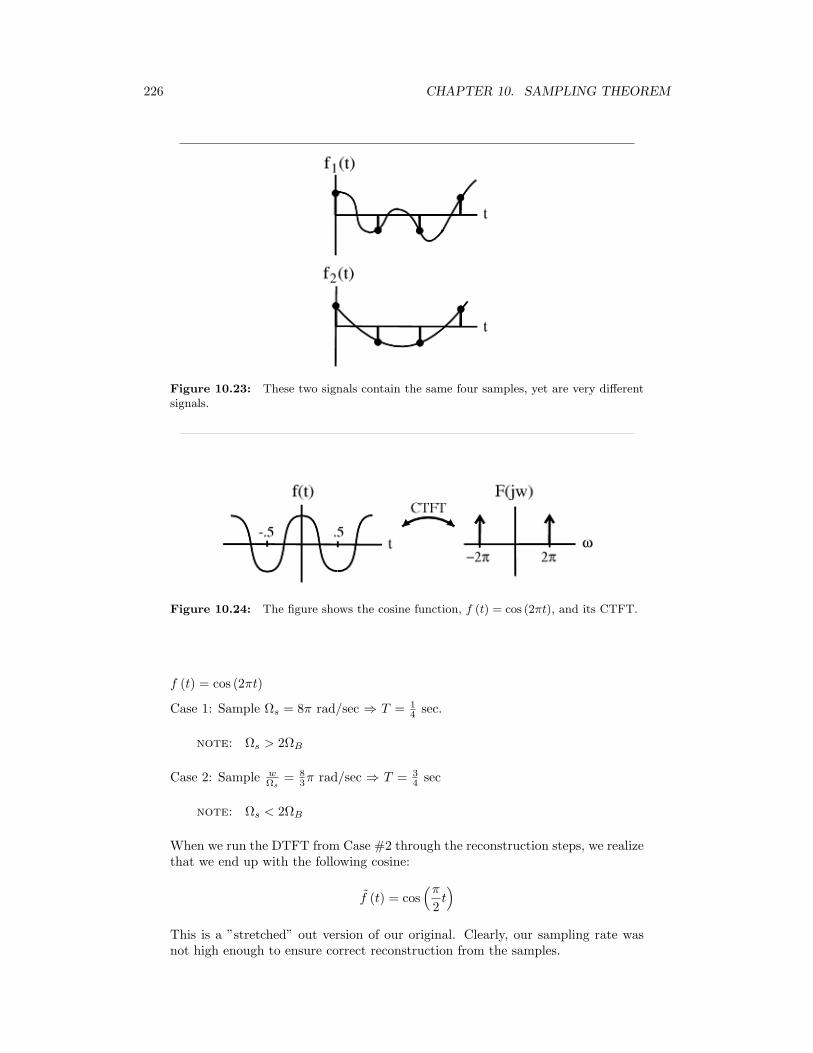
226 CHAPTER 10. SAMPLING THEOREM
Figure 10.23: These two signals contain the same four samples, yet are very differentsignals.
Figure 10.24: The figure shows the cosine function, f (t) = cos (2πt), and its CTFT.
f (t) = cos (2πt)
Case 1: Sample Ωs = 8π rad/sec ⇒ T = 14 sec.
note: Ωs > 2ΩB
Case 2: Sample wΩs
= 83π rad/sec ⇒ T = 3
4 sec
note: Ωs < 2ΩB
When we run the DTFT from Case #2 through the reconstruction steps, we realizethat we end up with the following cosine:
f (t) = cos(π
2t)
This is a ”stretched” out version of our original. Clearly, our sampling rate wasnot high enough to ensure correct reconstruction from the samples.
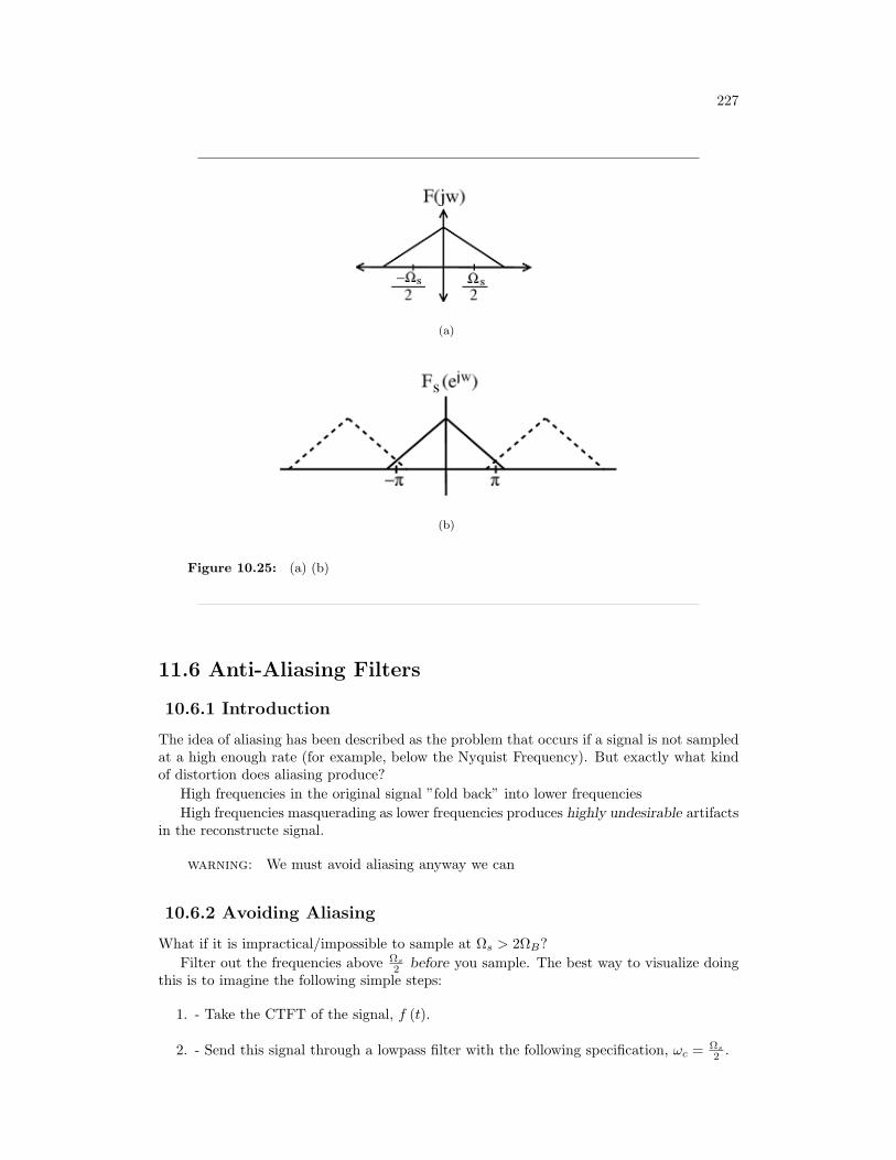
227
(a)
(b)
Figure 10.25: (a) (b)
11.6 Anti-Aliasing Filters
10.6.1 Introduction
The idea of aliasing has been described as the problem that occurs if a signal is not sampledat a high enough rate (for example, below the Nyquist Frequency). But exactly what kindof distortion does aliasing produce?
High frequencies in the original signal ”fold back” into lower frequenciesHigh frequencies masquerading as lower frequencies produces highly undesirable artifacts
in the reconstructe signal.
warning: We must avoid aliasing anyway we can
10.6.2 Avoiding Aliasing
What if it is impractical/impossible to sample at Ωs > 2ΩB?Filter out the frequencies above Ωs
2 before you sample. The best way to visualize doingthis is to imagine the following simple steps:
1. - Take the CTFT of the signal, f (t).
2. - Send this signal through a lowpass filter with the following specification, ωc = Ωs
2 .
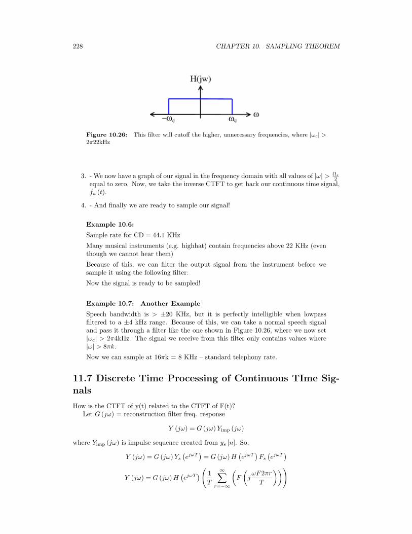
228 CHAPTER 10. SAMPLING THEOREM
Figure 10.26: This filter will cutoff the higher, unnecessary frequencies, where |ωc| >2π22kHz
3. - We now have a graph of our signal in the frequency domain with all values of |ω| > Ωs
2equal to zero. Now, we take the inverse CTFT to get back our continuous time signal,fa (t).
4. - And finally we are ready to sample our signal!
Example 10.6:
Sample rate for CD = 44.1 KHz
Many musical instruments (e.g. highhat) contain frequencies above 22 KHz (eventhough we cannot hear them)
Because of this, we can filter the output signal from the instrument before wesample it using the following filter:
Now the signal is ready to be sampled!
Example 10.7: Another Example
Speech bandwidth is > ±20 KHz, but it is perfectly intelligible when lowpassfiltered to a ±4 kHz range. Because of this, we can take a normal speech signaland pass it through a filter like the one shown in Figure 10.26, where we now set|ωc| > 2π4kHz. The signal we receive from this filter only contains values where|ω| > 8πk.
Now we can sample at 16πk = 8 KHz – standard telephony rate.
11.7 Discrete Time Processing of Continuous TIme Sig-nals
How is the CTFT of y(t) related to the CTFT of F(t)?Let G (jω) = reconstruction filter freq. response
Y (jω) = G (jω)Yimp (jω)
where Yimp (jω) is impulse sequence created from ys [n]. So,
Y (jω) = G (jω)Ys
(ejωT
)= G (jω)H
(ejωT
)Fs
(ejωT
)Y (jω) = G (jω)H
(ejωT
)( 1T
∞∑r=−∞
(F
(jωF2πrT
)))
229
Figure 10.27:
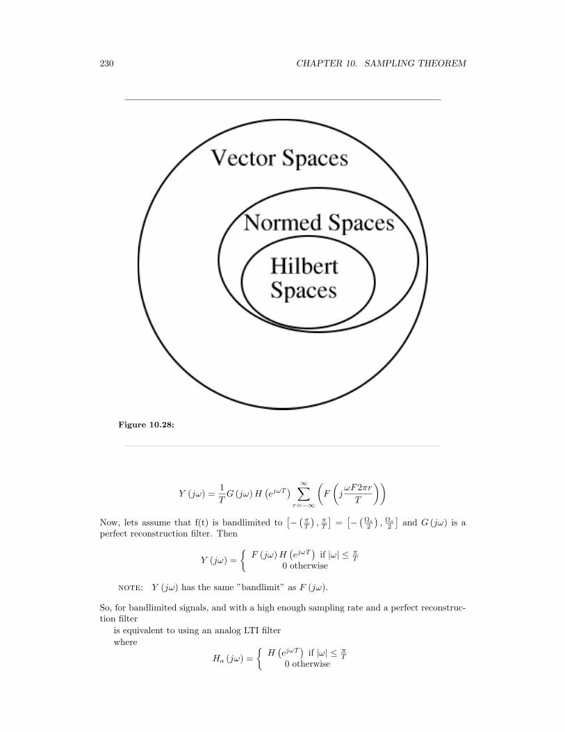
230 CHAPTER 10. SAMPLING THEOREM
Figure 10.28:
Y (jω) =1TG (jω)H
(ejωT
) ∞∑r=−∞
(F
(jωF2πrT
))Now, lets assume that f(t) is bandlimited to
[−(
πT
), π
T
]=[−(
Ωs
2
), Ωs
2
]and G (jω) is a
perfect reconstruction filter. Then
Y (jω) =F (jω)H
(ejωT
)if |ω| ≤ π
T0 otherwise
note: Y (jω) has the same ”bandlimit” as F (jω).
So, for bandlimited signals, and with a high enough sampling rate and a perfect reconstruc-tion filter
is equivalent to using an analog LTI filterwhere
Ha (jω) =H(ejωT
)if |ω| ≤ π
T0 otherwise
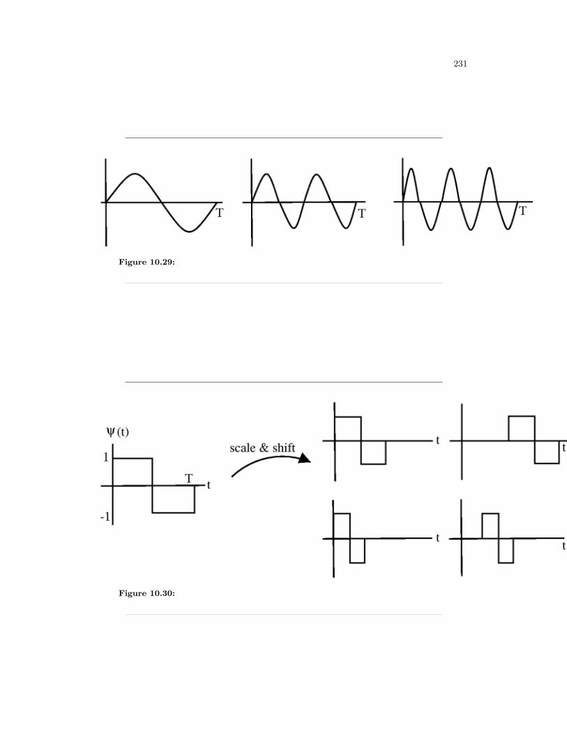
231
Figure 10.29:
Figure 10.30:
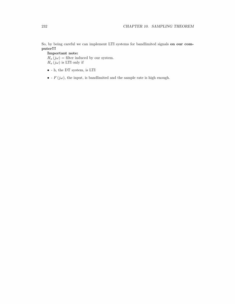
232 CHAPTER 10. SAMPLING THEOREM
So, by being careful we can implement LTI systems for bandlimited signals on our com-puter!!!
Important note:Ha (jω) = filter induced by our system.Ha (jω) is LTI only if
• - h, the DT system, is LTI
• - F (jω), the input, is bandlimited and the sample rate is high enough.
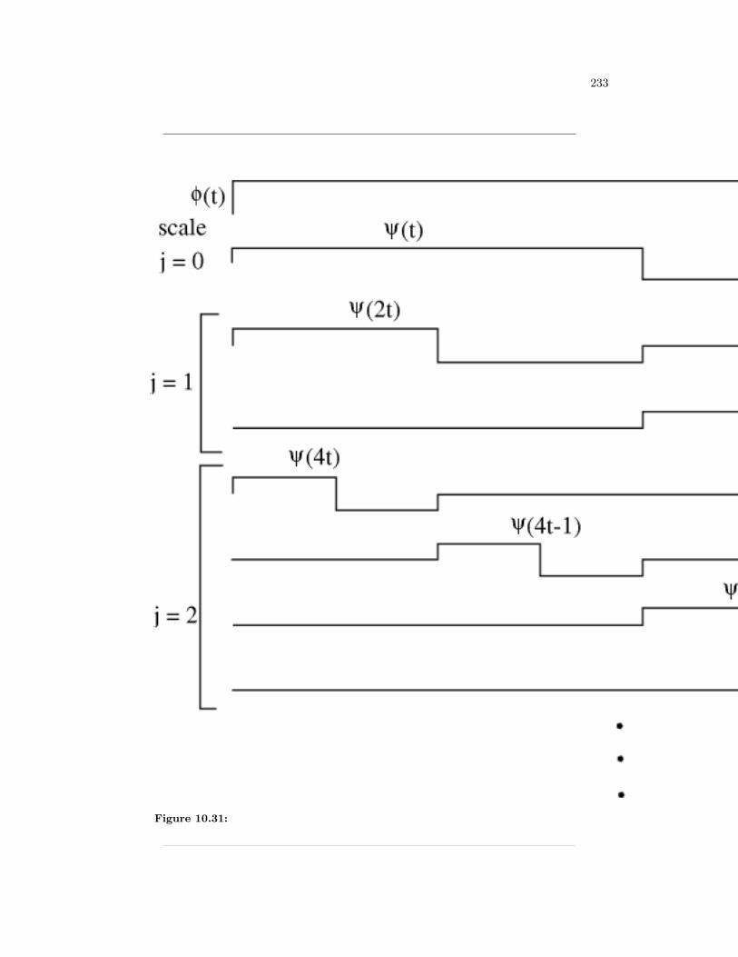
233
Figure 10.31:

234 CHAPTER 10. SAMPLING THEOREM
Chapter 11
Laplace Transform and SystemDesign
12.1 The Laplace Transforms
The Laplace transform is a generalization of the Continuous-Time Fourier Transform. How-ever, instead of using complex sinusoids of the form ejωt, as the CTFT does, the Laplacetransform uses the more general, est, where s = σ + jω.
Although Laplace transforms are rarely solved using integration (tables and computers(eg Matlab) are much more common), we will provide the bilateral Laplace transformpair here. These define the forward and inverse Laplace transformations. Notice the simi-larities between the forward and inverse transforms. This will give rise to many of the samesymmetries found in Fourier analysis.
Laplace Transform
F (s) =∫ ∞
−∞f (t) e−(st)dt (11.1)
Inverse Laplace Transform
f (t) =1
2πj
∫ c+j∞
c−j∞F (s) estds (11.2)
11.1.1 Finding the Laplace and Inverse Laplace Transforms
11.1.1.1 Solving the Integral
Probably the most difficult and least used method for finding the Laplace transform ofa signal is solving the integral. Although it is technically possible, it is extremely timeconsuming. Given how easy the next two methods are for finding it, we will not provideany more than this. The integrals are primarily there in order to understand where thefollowing methods originate from.
11.1.1.2 Using a Computer
Using a computer to find Laplace transforms is relatively painless. Matlab has two functions,laplace and ilaplace, that are both part of the symbolic toolbox, and will find the Laplace
235
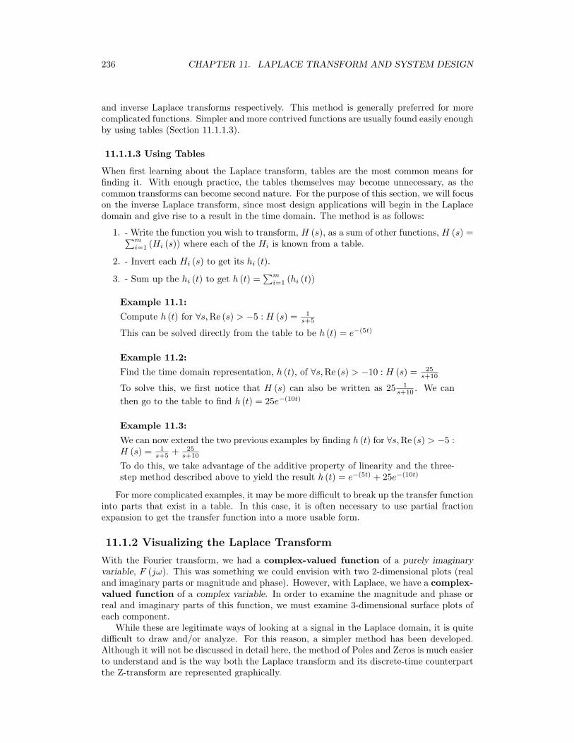
236 CHAPTER 11. LAPLACE TRANSFORM AND SYSTEM DESIGN
and inverse Laplace transforms respectively. This method is generally preferred for morecomplicated functions. Simpler and more contrived functions are usually found easily enoughby using tables (Section 11.1.1.3).
11.1.1.3 Using Tables
When first learning about the Laplace transform, tables are the most common means forfinding it. With enough practice, the tables themselves may become unnecessary, as thecommon transforms can become second nature. For the purpose of this section, we will focuson the inverse Laplace transform, since most design applications will begin in the Laplacedomain and give rise to a result in the time domain. The method is as follows:
1. - Write the function you wish to transform, H (s), as a sum of other functions, H (s) =∑mi=1 (Hi (s)) where each of the Hi is known from a table.
2. - Invert each Hi (s) to get its hi (t).
3. - Sum up the hi (t) to get h (t) =∑m
i=1 (hi (t))
Example 11.1:
Compute h (t) for ∀s,Re (s) > −5 : H (s) = 1s+5
This can be solved directly from the table to be h (t) = e−(5t)
Example 11.2:
Find the time domain representation, h (t), of ∀s,Re (s) > −10 : H (s) = 25s+10
To solve this, we first notice that H (s) can also be written as 25 1s+10 . We can
then go to the table to find h (t) = 25e−(10t)
Example 11.3:
We can now extend the two previous examples by finding h (t) for ∀s,Re (s) > −5 :H (s) = 1
s+5 + 25s+10
To do this, we take advantage of the additive property of linearity and the three-step method described above to yield the result h (t) = e−(5t) + 25e−(10t)
For more complicated examples, it may be more difficult to break up the transfer functioninto parts that exist in a table. In this case, it is often necessary to use partial fractionexpansion to get the transfer function into a more usable form.
11.1.2 Visualizing the Laplace Transform
With the Fourier transform, we had a complex-valued function of a purely imaginaryvariable, F (jω). This was something we could envision with two 2-dimensional plots (realand imaginary parts or magnitude and phase). However, with Laplace, we have a complex-valued function of a complex variable. In order to examine the magnitude and phase orreal and imaginary parts of this function, we must examine 3-dimensional surface plots ofeach component.
While these are legitimate ways of looking at a signal in the Laplace domain, it is quitedifficult to draw and/or analyze. For this reason, a simpler method has been developed.Although it will not be discussed in detail here, the method of Poles and Zeros is much easierto understand and is the way both the Laplace transform and its discrete-time counterpartthe Z-transform are represented graphically.
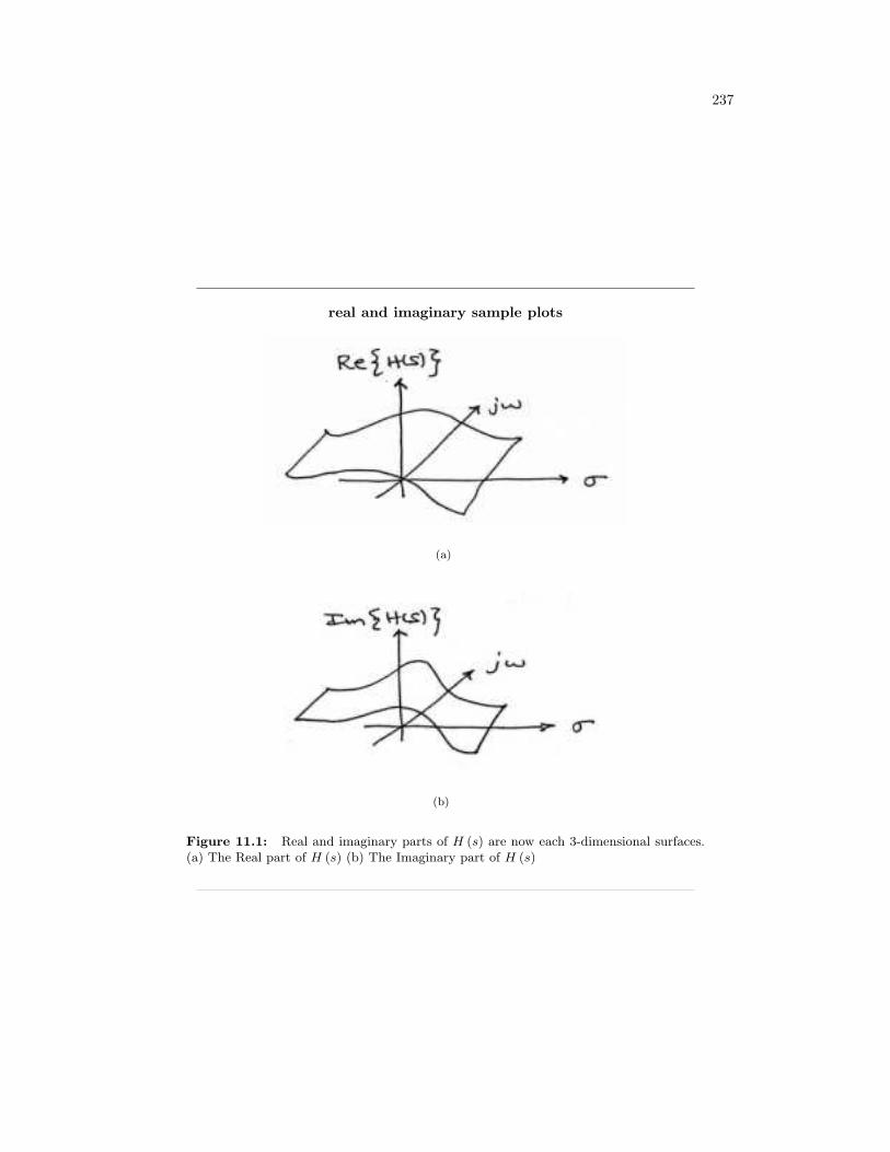
237
real and imaginary sample plots
(a)
(b)
Figure 11.1: Real and imaginary parts of H (s) are now each 3-dimensional surfaces.(a) The Real part of H (s) (b) The Imaginary part of H (s)
238 CHAPTER 11. LAPLACE TRANSFORM AND SYSTEM DESIGN
magnitude and phase sample plots
(a)
(b)
Figure 11.2: Magnitude and phase of H (s) are also each 3-dimensional surfaces. Thisrepresentation is more common than real and imaginary parts. (a) The Magnitude ofH (s) (b) The Phase of H (s)
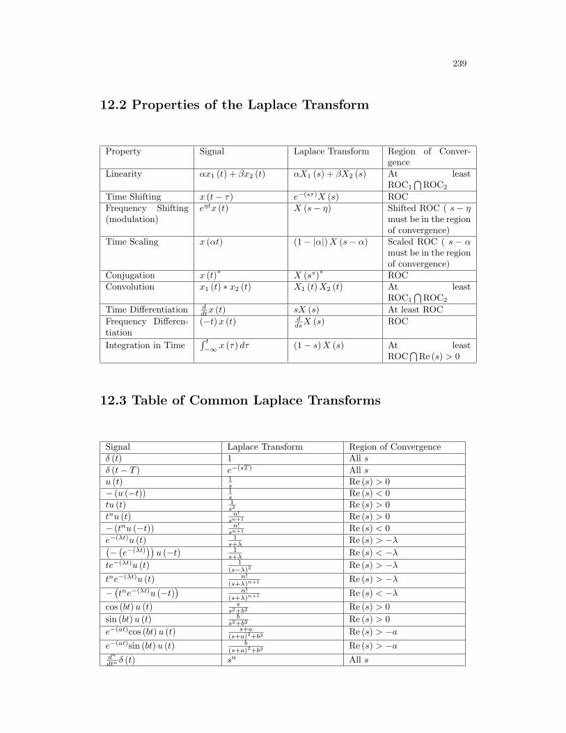
239
12.2 Properties of the Laplace Transform
Property Signal Laplace Transform Region of Conver-gence
Linearity αx1 (t) + βx2 (t) αX1 (s) + βX2 (s) At leastROC1
⋂ROC2
Time Shifting x (t− τ) e−(sτ)X (s) ROCFrequency Shifting(modulation)
eηtx (t) X (s− η) Shifted ROC ( s − ηmust be in the regionof convergence)
Time Scaling x (αt) (1− |α|)X (s− α) Scaled ROC ( s − αmust be in the regionof convergence)
Conjugation x (t)∗ X (s∗)∗ ROCConvolution x1 (t) ∗ x2 (t) X1 (t)X2 (t) At least
ROC1
⋂ROC2
Time Differentiation ddtx (t) sX (s) At least ROC
Frequency Differen-tiation
(−t)x (t) ddsX (s) ROC
Integration in Time∫ t
−∞ x (τ) dτ (1− s)X (s) At leastROC
⋂Re (s) > 0
12.3 Table of Common Laplace Transforms
Signal Laplace Transform Region of Convergenceδ (t) 1 All sδ (t− T ) e−(sT ) All su (t) 1
s Re (s) > 0− (u (−t)) 1
s Re (s) < 0tu (t) 1
s2 Re (s) > 0tnu (t) n!
sn+1 Re (s) > 0− (tnu (−t)) n!
sn+1 Re (s) < 0e−(λt)u (t) 1
s+λ Re (s) > −λ(−(e−(λt)
))u (−t) 1
s+λ Re (s) < −λte−(λt)u (t) 1
(s−λ)2Re (s) > −λ
tne−(λt)u (t) n!(s+λ)n+1 Re (s) > −λ
−(tne−(λt)u (−t)
)n!
(s+λ)n+1 Re (s) < −λcos (bt)u (t) s
s2+b2 Re (s) > 0sin (bt)u (t) b
s2+b2 Re (s) > 0e−(at)cos (bt)u (t) s+a
(s+a)2+b2Re (s) > −a
e−(at)sin (bt)u (t) b(s+a)2+b2
Re (s) > −adn
dtn δ (t) sn All s
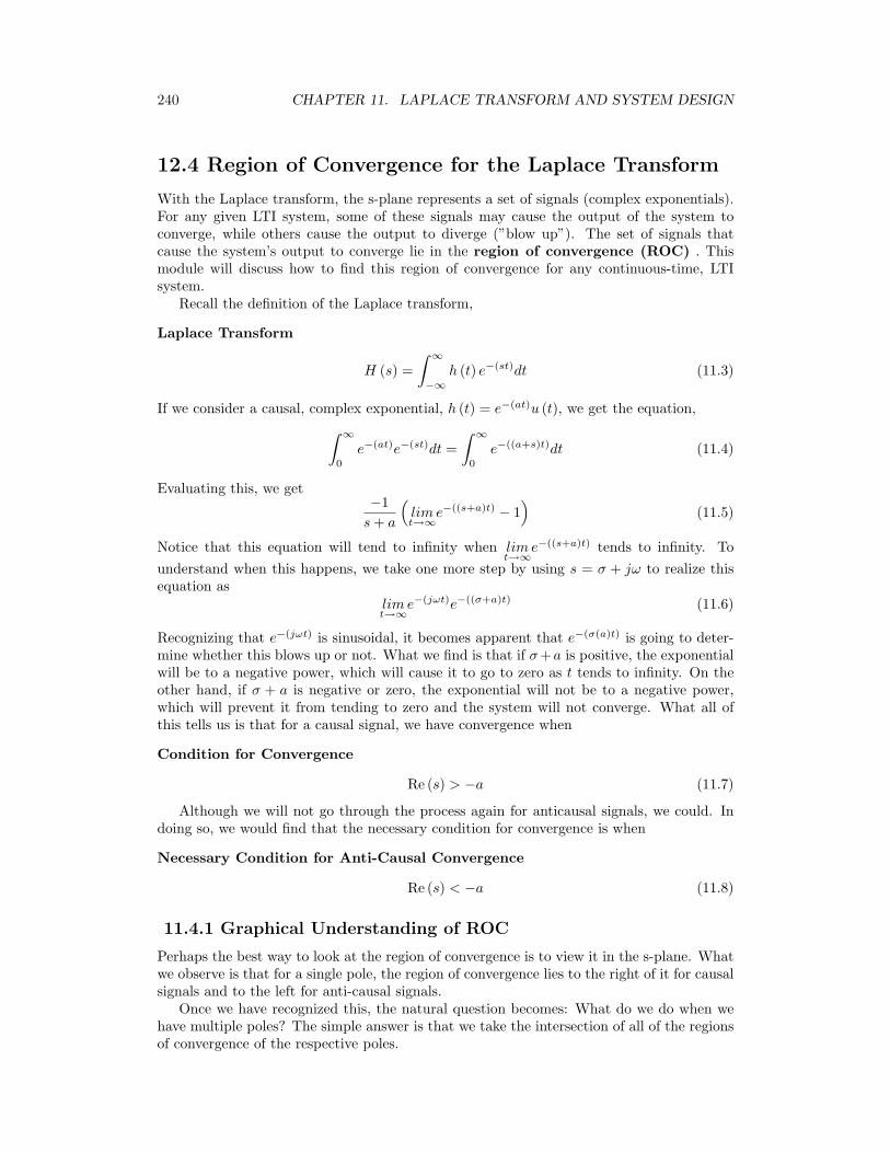
240 CHAPTER 11. LAPLACE TRANSFORM AND SYSTEM DESIGN
12.4 Region of Convergence for the Laplace Transform
With the Laplace transform, the s-plane represents a set of signals (complex exponentials).For any given LTI system, some of these signals may cause the output of the system toconverge, while others cause the output to diverge (”blow up”). The set of signals thatcause the system’s output to converge lie in the region of convergence (ROC) . Thismodule will discuss how to find this region of convergence for any continuous-time, LTIsystem.
Recall the definition of the Laplace transform,
Laplace Transform
H (s) =∫ ∞
−∞h (t) e−(st)dt (11.3)
If we consider a causal, complex exponential, h (t) = e−(at)u (t), we get the equation,∫ ∞
0
e−(at)e−(st)dt =∫ ∞
0
e−((a+s)t)dt (11.4)
Evaluating this, we get−1s+ a
(limt→∞
e−((s+a)t) − 1)
(11.5)
Notice that this equation will tend to infinity when limt→∞
e−((s+a)t) tends to infinity. Tounderstand when this happens, we take one more step by using s = σ + jω to realize thisequation as
limt→∞
e−(jωt)e−((σ+a)t) (11.6)
Recognizing that e−(jωt) is sinusoidal, it becomes apparent that e−(σ(a)t) is going to deter-mine whether this blows up or not. What we find is that if σ+a is positive, the exponentialwill be to a negative power, which will cause it to go to zero as t tends to infinity. On theother hand, if σ + a is negative or zero, the exponential will not be to a negative power,which will prevent it from tending to zero and the system will not converge. What all ofthis tells us is that for a causal signal, we have convergence when
Condition for Convergence
Re (s) > −a (11.7)
Although we will not go through the process again for anticausal signals, we could. Indoing so, we would find that the necessary condition for convergence is when
Necessary Condition for Anti-Causal Convergence
Re (s) < −a (11.8)
11.4.1 Graphical Understanding of ROC
Perhaps the best way to look at the region of convergence is to view it in the s-plane. Whatwe observe is that for a single pole, the region of convergence lies to the right of it for causalsignals and to the left for anti-causal signals.
Once we have recognized this, the natural question becomes: What do we do when wehave multiple poles? The simple answer is that we take the intersection of all of the regionsof convergence of the respective poles.
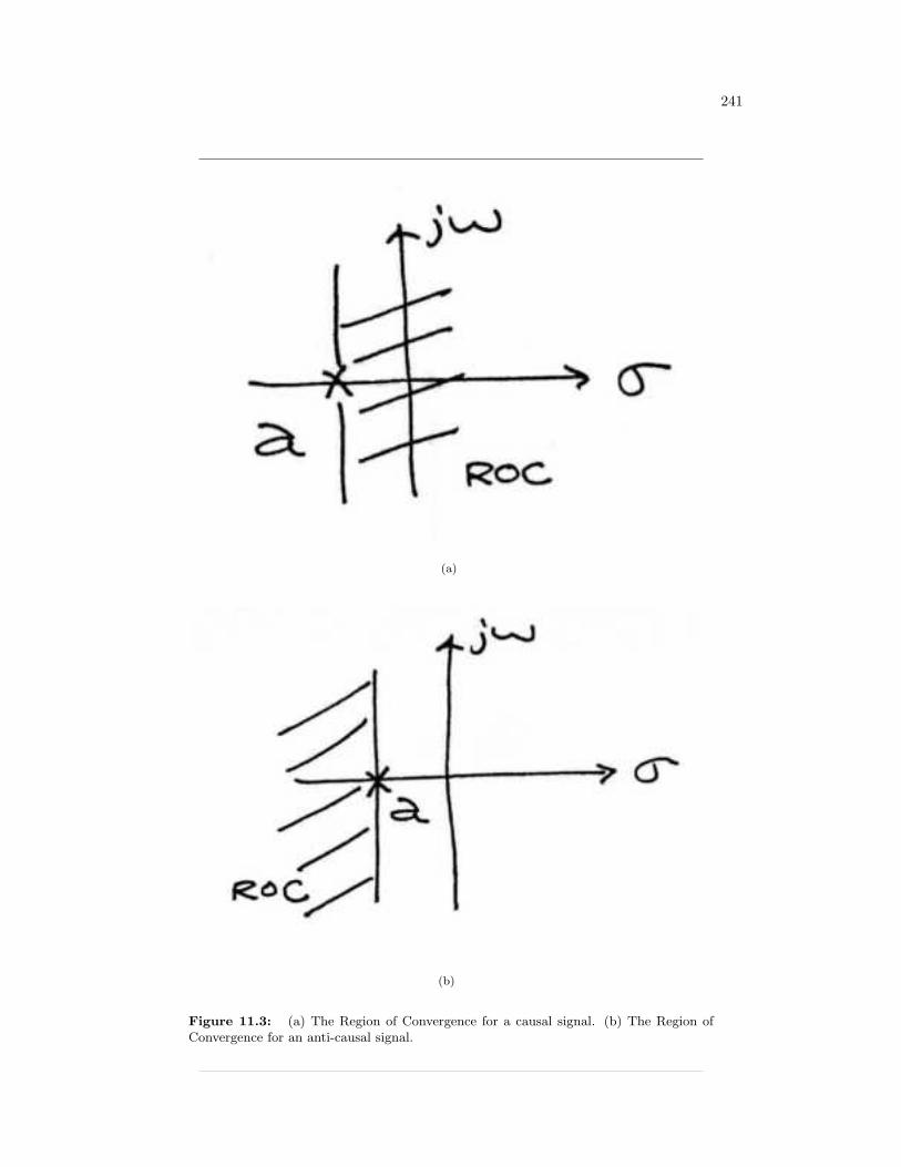
241
(a)
(b)
Figure 11.3: (a) The Region of Convergence for a causal signal. (b) The Region ofConvergence for an anti-causal signal.
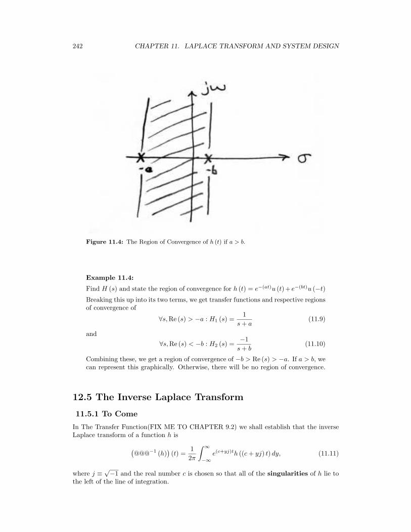
242 CHAPTER 11. LAPLACE TRANSFORM AND SYSTEM DESIGN
Figure 11.4: The Region of Convergence of h (t) if a > b.
Example 11.4:
Find H (s) and state the region of convergence for h (t) = e−(at)u (t)+ e−(bt)u (−t)Breaking this up into its two terms, we get transfer functions and respective regionsof convergence of
∀s,Re (s) > −a : H1 (s) =1
s+ a(11.9)
and∀s,Re (s) < −b : H2 (s) =
−1s+ b
(11.10)
Combining these, we get a region of convergence of −b > Re (s) > −a. If a > b, wecan represent this graphically. Otherwise, there will be no region of convergence.
12.5 The Inverse Laplace Transform
11.5.1 To Come
In The Transfer Function(FIX ME TO CHAPTER 9.2) we shall establish that the inverseLaplace transform of a function h is
(@@@−1 (h)
)(t) =
12π
∫ ∞
−∞e(c+yj)th ((c+ yj) t) dy, (11.11)
where j ≡√−1 and the real number c is chosen so that all of the singularities of h lie to
the left of the line of integration.
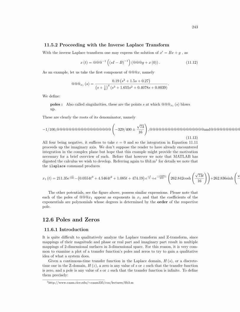
243
11.5.2 Proceeding with the Inverse Laplace Transform
With the inverse Laplace transform one may express the solution of x′ = Bx+ g , as
x (t) = @@@−1((sI −B)−1
)(@@@g + x (0)) . (11.12)
As an example, let us take the first component of @@@x, namely
@@@x1 (s) =0.19
(s2 + 1.5s+ 0.27
)(s+ 1
6
)4 (s3 + 1.655s2 + 0.4078s+ 0.0039).
We define:
poles : Also called singularities, these are the points s at which @@@x1 (s) blowsup.
These are clearly the roots of its denominator, namely
−1/100,@@@@@@@@@@@@@@@@@@
(−329/400±
√73
16
),@@@@@@@@@@@@@@@@@@and@@@@@@@@@@@@@@@@@@−1/6.
(11.13)All four being negative, it suffices to take c = 0 and so the integration in Equation 11.11proceeds up the imaginary axis. We don’t suppose the reader to have already encounteredintegration in the complex plane but hope that this example might provide the motivationnecessary for a brief overview of such. Before that however we note that MATLAB hasdigested the calculus we wish to develop. Referring again to fib3.m1 for details we note thatthe ilaplace command produces
x1 (t) = 211.35e−t100−
(0.0554t3 + 4.5464t2 + 1.085t+ 474.19
)e−t6 +e
−(329t)400
(262.842cosh
(√73t16
))+262.836sinh
(√73t16
)
The other potentials, see the figure above, possess similar expressions. Please note thateach of the poles of @@@x1 appear as exponents in x1 and that the coefficients of theexponentials are polynomials whose degrees is determined by the order of the respectivepole.
12.6 Poles and Zeros
11.6.1 Introduction
It is quite difficult to qualitatively analyze the Laplace transform and Z-transform, sincemappings of their magnitude and phase or real part and imaginary part result in multiplemappings of 2-dimensional surfaces in 3-dimensional space. For this reason, it is very com-mon to examine a plot of a transfer function’s poles and zeros to try to gain a qualitativeidea of what a system does.
Given a continuous-time transfer function in the Laplace domain, H (s), or a discrete-time one in the Z-domain, H (z), a zero is any value of s or z such that the transfer functionis zero, and a pole is any value of s or z such that the transfer function is infinite. To definethem precisely:
1http://www.caam.rice.edu/∼caam335/cox/lectures/fib3.m
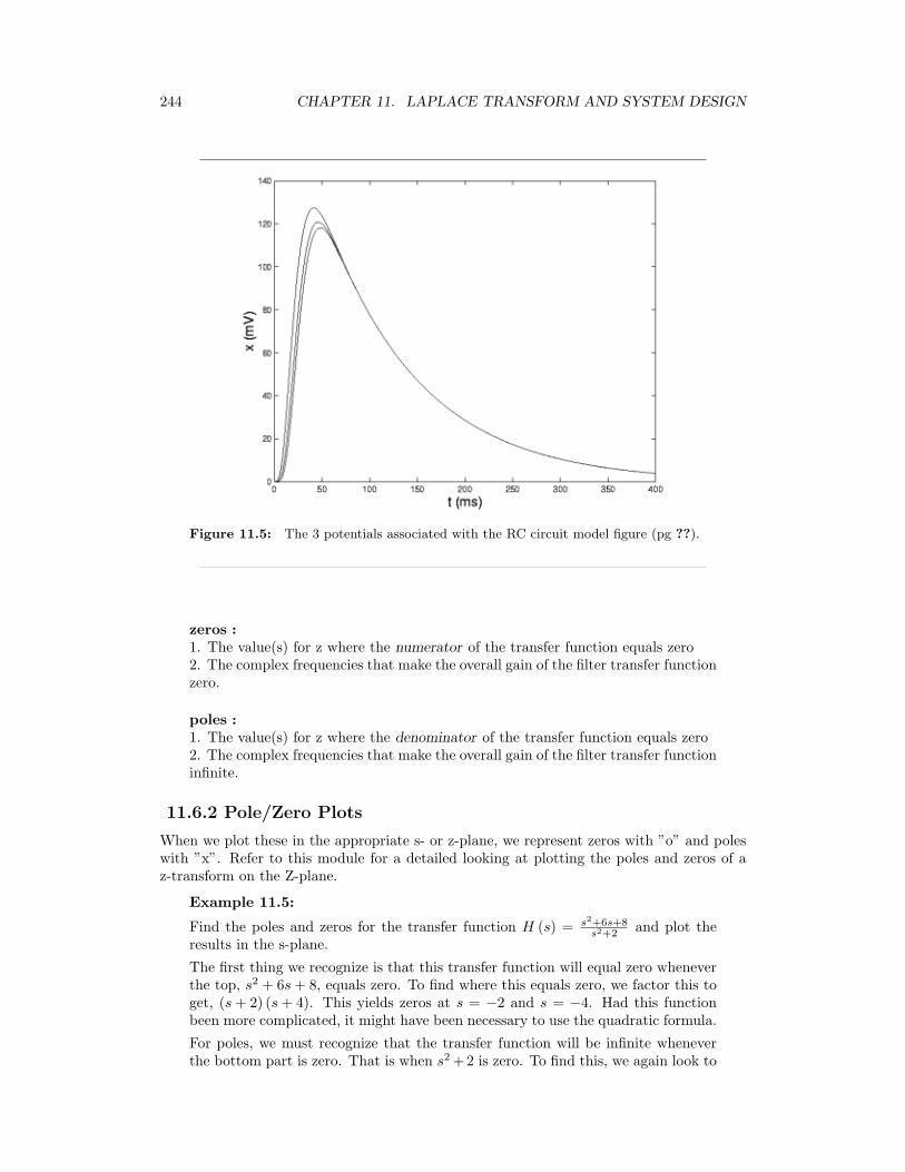
244 CHAPTER 11. LAPLACE TRANSFORM AND SYSTEM DESIGN
Figure 11.5: The 3 potentials associated with the RC circuit model figure (pg ??).
zeros :1. The value(s) for z where the numerator of the transfer function equals zero2. The complex frequencies that make the overall gain of the filter transfer functionzero.
poles :1. The value(s) for z where the denominator of the transfer function equals zero2. The complex frequencies that make the overall gain of the filter transfer functioninfinite.
11.6.2 Pole/Zero Plots
When we plot these in the appropriate s- or z-plane, we represent zeros with ”o” and poleswith ”x”. Refer to this module for a detailed looking at plotting the poles and zeros of az-transform on the Z-plane.
Example 11.5:
Find the poles and zeros for the transfer function H (s) = s2+6s+8s2+2 and plot the
results in the s-plane.
The first thing we recognize is that this transfer function will equal zero wheneverthe top, s2 + 6s+ 8, equals zero. To find where this equals zero, we factor this toget, (s+ 2) (s+ 4). This yields zeros at s = −2 and s = −4. Had this functionbeen more complicated, it might have been necessary to use the quadratic formula.
For poles, we must recognize that the transfer function will be infinite wheneverthe bottom part is zero. That is when s2 +2 is zero. To find this, we again look to
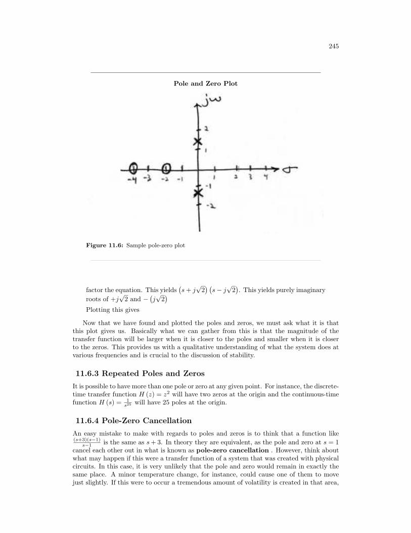
245
Pole and Zero Plot
Figure 11.6: Sample pole-zero plot
factor the equation. This yields(s+ j
√2) (s− j
√2). This yields purely imaginary
roots of +j√
2 and −(j√
2)
Plotting this gives
Now that we have found and plotted the poles and zeros, we must ask what it is thatthis plot gives us. Basically what we can gather from this is that the magnitude of thetransfer function will be larger when it is closer to the poles and smaller when it is closerto the zeros. This provides us with a qualitative understanding of what the system does atvarious frequencies and is crucial to the discussion of stability.
11.6.3 Repeated Poles and Zeros
It is possible to have more than one pole or zero at any given point. For instance, the discrete-time transfer function H (z) = z2 will have two zeros at the origin and the continuous-timefunction H (s) = 1
s25 will have 25 poles at the origin.
11.6.4 Pole-Zero Cancellation
An easy mistake to make with regards to poles and zeros is to think that a function like(s+3)(s−1)
s−1 is the same as s+ 3. In theory they are equivalent, as the pole and zero at s = 1cancel each other out in what is known as pole-zero cancellation . However, think aboutwhat may happen if this were a transfer function of a system that was created with physicalcircuits. In this case, it is very unlikely that the pole and zero would remain in exactly thesame place. A minor temperature change, for instance, could cause one of them to movejust slightly. If this were to occur a tremendous amount of volatility is created in that area,
246 CHAPTER 11. LAPLACE TRANSFORM AND SYSTEM DESIGN
since there is a change from infinity at the pole to zero at the zero in a very small range ofsignals. This is generally a very bad way to try to eliminate a pole. A much better way isto use control theory to move the pole to a better place.
Chapter 12
Z-Transform and DigitalFiltering
13.1 The Z Transform: Definition
12.1.1 Basic Definition of the Z-Transform
The z-transform of a sequence is defined as
X (z) =∞∑
n=−∞
(x [n] z−n
)(12.1)
Sometimes this equation is referred to as the bilateral z-transform . At times the z-transform is defined as
X (z) =∞∑
n=0
(x [n] z−n
)(12.2)
which is known as the unilateral z-transform .There is a close relationship between the z-transform and the Fourier transform of a
discrete time signal, which is defined as
X(ejω)
=∞∑
n=−∞
(x [n] e−(jωn)
)(12.3)
Notice that that when the z−n is replaced with e−(jωn) the z-transform reduces to theFourier Transform. When the Fourier Transform exists, z = ejω , which is to have themagnitude of z equal to unity.
12.1.2 The Complex Plane
In order to get further insight into the relationship between the Fourier Transform and theZ-Transform it is useful to look at the complex plane or z-plane . Take a look at thecomplex plane:
The Z-plane is a complex plane with an imaginary and real axis referring to the complex-valued variable z. The position on the complex plane is given by rejω , and the angle fromthe positive, real axis around the plane is denoted by ω. X (z) is defined everywhere on thisplane. X
(ejω)on the other hand is defined only where |z| = 1, which is refered to as the
247
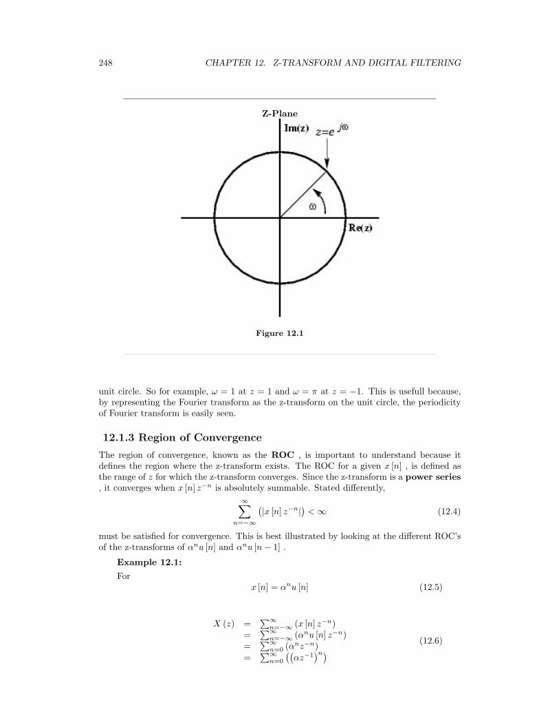
248 CHAPTER 12. Z-TRANSFORM AND DIGITAL FILTERING
Z-Plane
Figure 12.1
unit circle. So for example, ω = 1 at z = 1 and ω = π at z = −1. This is usefull because,by representing the Fourier transform as the z-transform on the unit circle, the periodicityof Fourier transform is easily seen.
12.1.3 Region of Convergence
The region of convergence, known as the ROC , is important to understand because itdefines the region where the z-transform exists. The ROC for a given x [n] , is defined asthe range of z for which the z-transform converges. Since the z-transform is a power series, it converges when x [n] z−n is absolutely summable. Stated differently,
∞∑n=−∞
(|x [n] z−n|
)<∞ (12.4)
must be satisfied for convergence. This is best illustrated by looking at the different ROC’sof the z-transforms of αnu [n] and αnu [n− 1] .
Example 12.1:
Forx [n] = αnu [n] (12.5)
X (z) =∑∞
n=−∞ (x [n] z−n)=
∑∞n=−∞ (αnu [n] z−n)
=∑∞
n=0 (αnz−n)=
∑∞n=0
((αz−1
)n) (12.6)
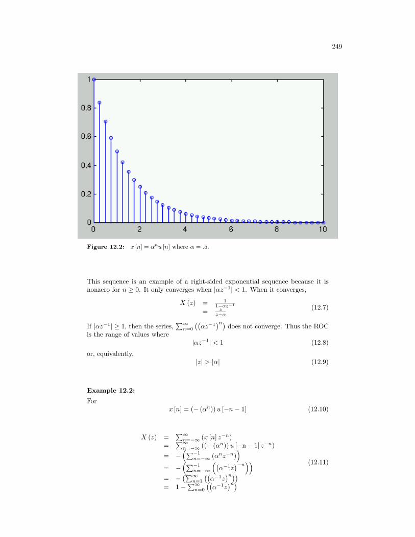
249
Figure 12.2: x [n] = αnu [n] where α = .5.
This sequence is an example of a right-sided exponential sequence because it isnonzero for n ≥ 0. It only converges when |αz−1| < 1. When it converges,
X (z) = 11−αz−1
= zz−α
(12.7)
If |αz−1| ≥ 1, then the series,∑∞
n=0
((αz−1
)n) does not converge. Thus the ROCis the range of values where
|αz−1| < 1 (12.8)
or, equivalently,|z| > |α| (12.9)
Example 12.2:
Forx [n] = (− (αn))u [−n− 1] (12.10)
X (z) =∑∞
n=−∞ (x [n] z−n)=
∑∞n=−∞ ((− (αn))u [−n− 1] z−n)
= −(∑−1
n=−∞ (αnz−n))
= −(∑−1
n=−∞
((α−1z
)−n))
= −(∑∞
n=1
((α−1z
)n))= 1−
∑∞n=0
((α−1z
)n)(12.11)
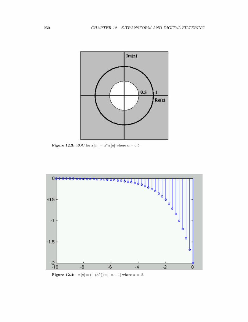
250 CHAPTER 12. Z-TRANSFORM AND DIGITAL FILTERING
Figure 12.3: ROC for x [n] = αnu [n] where α = 0.5
Figure 12.4: x [n] = (− (αn)) u [−n− 1] where α = .5.
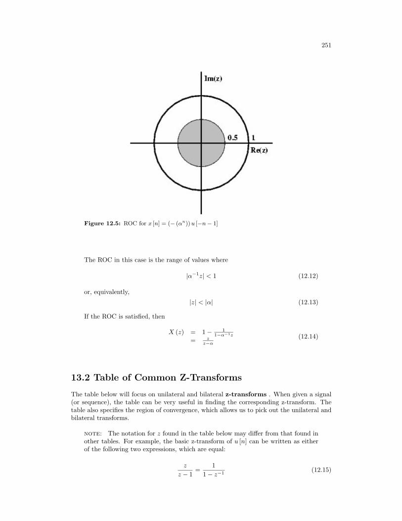
251
Figure 12.5: ROC for x [n] = (− (αn)) u [−n− 1]
The ROC in this case is the range of values where
|α−1z| < 1 (12.12)
or, equivalently,
|z| < |α| (12.13)
If the ROC is satisfied, then
X (z) = 1− 11−α−1z
= zz−α
(12.14)
13.2 Table of Common Z-Transforms
The table below will focus on unilateral and bilateral z-transforms . When given a signal(or sequence), the table can be very useful in finding the corresponding z-transform. Thetable also specifies the region of convergence, which allows us to pick out the unilateral andbilateral transforms.
note: The notation for z found in the table below may differ from that found inother tables. For example, the basic z-transform of u [n] can be written as eitherof the following two expressions, which are equal:
z
z − 1=
11− z−1
(12.15)
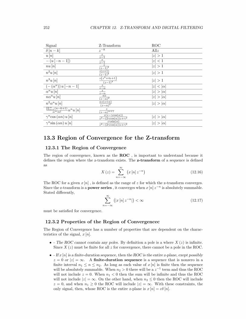
252 CHAPTER 12. Z-TRANSFORM AND DIGITAL FILTERING
Signal Z-Transform ROCδ [n− k] z−k Allzu [n] z
z−1 |z| > 1− (u [−n− 1]) z
z−1 |z| < 1nu [n] z
(z−1)2|z| > 1
n2u [n] z(z+1)
(z−1)3|z| > 1
n3u [n]z(z2+4z+1)
(z−1)4|z| > 1
(− (αn))u [−n− 1] zz−α |z| < |α|
αnu [n] zz−α |z| > |α|
nαnu [n] αz(z−α)2
|z| > |α|n2αnu [n] αz(z+α)
(z−α)3|z| > |α|∏m
k=1(n−k+1)
αmm! αnu [n] z(z−α)m+1
γncos (αn)u [n] z(z−γcos(α))z2−(2γcos(α))z+γ2 |z| > |α|
γnsin (αn)u [n] zγsin(α)z2−(2γcos(α))z+γ2 |z| > |α|
13.3 Region of Convergence for the Z-transform
12.3.1 The Region of Convergence
The region of convergence, known as the ROC , is important to understand because itdefines the region where the z-transform exists. The z-transform of a sequence is definedas
X (z) =∞∑
n=−∞
(x [n] z−n
)(12.16)
The ROC for a given x [n] , is defined as the range of z for which the z-transform converges.Since the z-transform is a power series , it converges when x [n] z−n is absolutely summable.Stated differently,
∞∑n=−∞
(|x [n] z−n|
)<∞ (12.17)
must be satisfied for convergence.
12.3.2 Properties of the Region of Convergencec
The Region of Convergence has a number of properties that are dependent on the charac-teristics of the signal, x [n].
• - The ROC cannot contain any poles. By definition a pole is a where X (z) is infinite.Since X (z) must be finite for all z for convergence, there cannot be a pole in the ROC.
• - If x [n] is a finite-duration sequence, then the ROC is the entire z-plane, exept possiblyz = 0 or |z| = ∞. A finite-duration sequence is a sequence that is nonzero in afinite interval n1 ≤ n ≤ n2. As long as each value of x [n] is finite then the sequencewill be absolutely summable. When n2 > 0 there will be a z−1 term and thus the ROCwill not include z = 0. When n1 < 0 then the sum will be infinite and thus the ROCwill not include |z| = ∞. On the other hand, when n2 ≤ 0 then the ROC will includez = 0, and when n1 ≥ 0 the ROC will include |z| = ∞. With these constraints, theonly signal, then, whose ROC is the entire z-plane is x [n] = cδ [n].
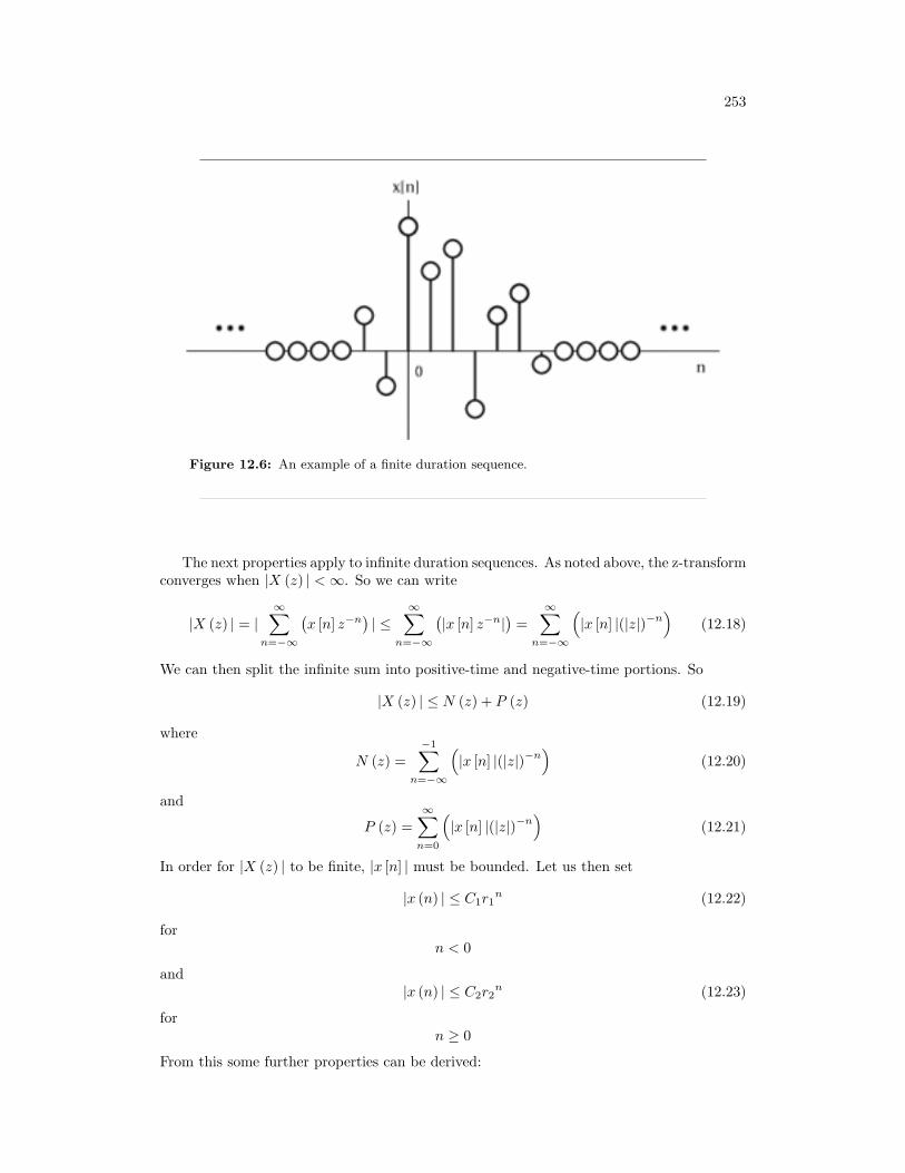
253
Figure 12.6: An example of a finite duration sequence.
The next properties apply to infinite duration sequences. As noted above, the z-transformconverges when |X (z) | <∞. So we can write
|X (z) | = |∞∑
n=−∞
(x [n] z−n
)| ≤
∞∑n=−∞
(|x [n] z−n|
)=
∞∑n=−∞
(|x [n] |(|z|)−n
)(12.18)
We can then split the infinite sum into positive-time and negative-time portions. So
|X (z) | ≤ N (z) + P (z) (12.19)
where
N (z) =−1∑
n=−∞
(|x [n] |(|z|)−n
)(12.20)
and
P (z) =∞∑
n=0
(|x [n] |(|z|)−n
)(12.21)
In order for |X (z) | to be finite, |x [n] | must be bounded. Let us then set
|x (n) | ≤ C1r1n (12.22)
forn < 0
and|x (n) | ≤ C2r2
n (12.23)
forn ≥ 0
From this some further properties can be derived:
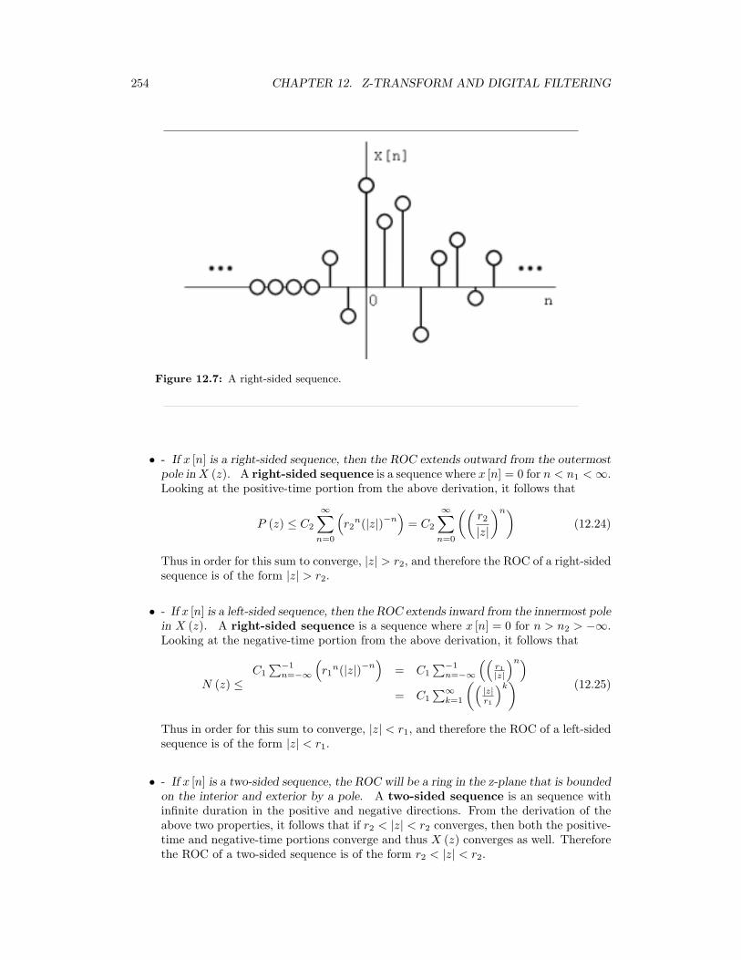
254 CHAPTER 12. Z-TRANSFORM AND DIGITAL FILTERING
Figure 12.7: A right-sided sequence.
• - If x [n] is a right-sided sequence, then the ROC extends outward from the outermostpole inX (z). A right-sided sequence is a sequence where x [n] = 0 for n < n1 <∞.Looking at the positive-time portion from the above derivation, it follows that
P (z) ≤ C2
∞∑n=0
(r2
n(|z|)−n)
= C2
∞∑n=0
((r2|z|
)n)(12.24)
Thus in order for this sum to converge, |z| > r2, and therefore the ROC of a right-sidedsequence is of the form |z| > r2.
• - If x [n] is a left-sided sequence, then the ROC extends inward from the innermost polein X (z). A right-sided sequence is a sequence where x [n] = 0 for n > n2 > −∞.Looking at the negative-time portion from the above derivation, it follows that
N (z) ≤C1
∑−1n=−∞
(r1
n(|z|)−n)
= C1
∑−1n=−∞
((r1|z|
)n)= C1
∑∞k=1
((|z|r1
)k) (12.25)
Thus in order for this sum to converge, |z| < r1, and therefore the ROC of a left-sidedsequence is of the form |z| < r1.
• - If x [n] is a two-sided sequence, the ROC will be a ring in the z-plane that is boundedon the interior and exterior by a pole. A two-sided sequence is an sequence withinfinite duration in the positive and negative directions. From the derivation of theabove two properties, it follows that if r2 < |z| < r2 converges, then both the positive-time and negative-time portions converge and thus X (z) converges as well. Thereforethe ROC of a two-sided sequence is of the form r2 < |z| < r2.
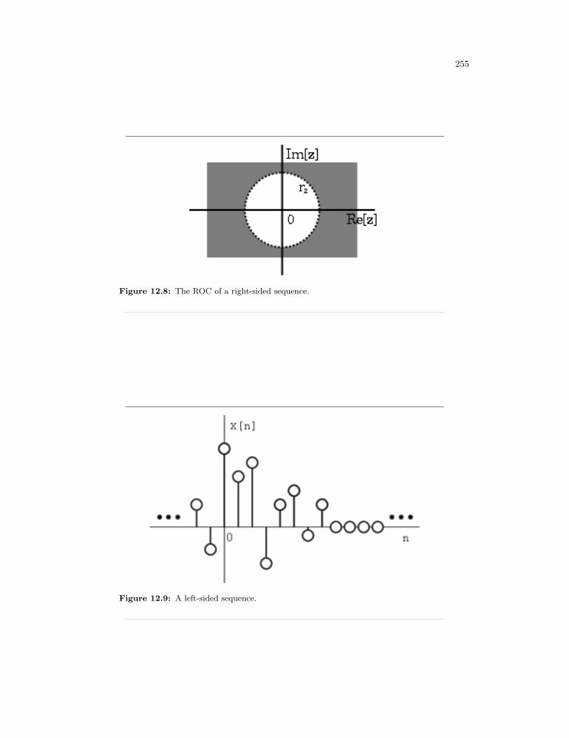
255
Figure 12.8: The ROC of a right-sided sequence.
Figure 12.9: A left-sided sequence.
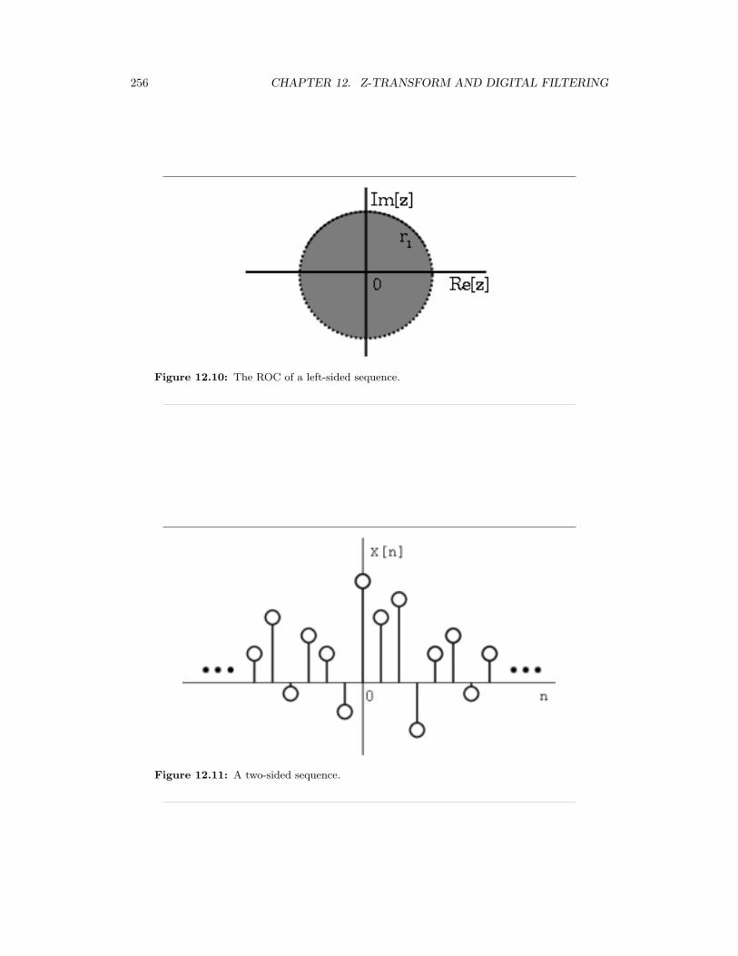
256 CHAPTER 12. Z-TRANSFORM AND DIGITAL FILTERING
Figure 12.10: The ROC of a left-sided sequence.
Figure 12.11: A two-sided sequence.
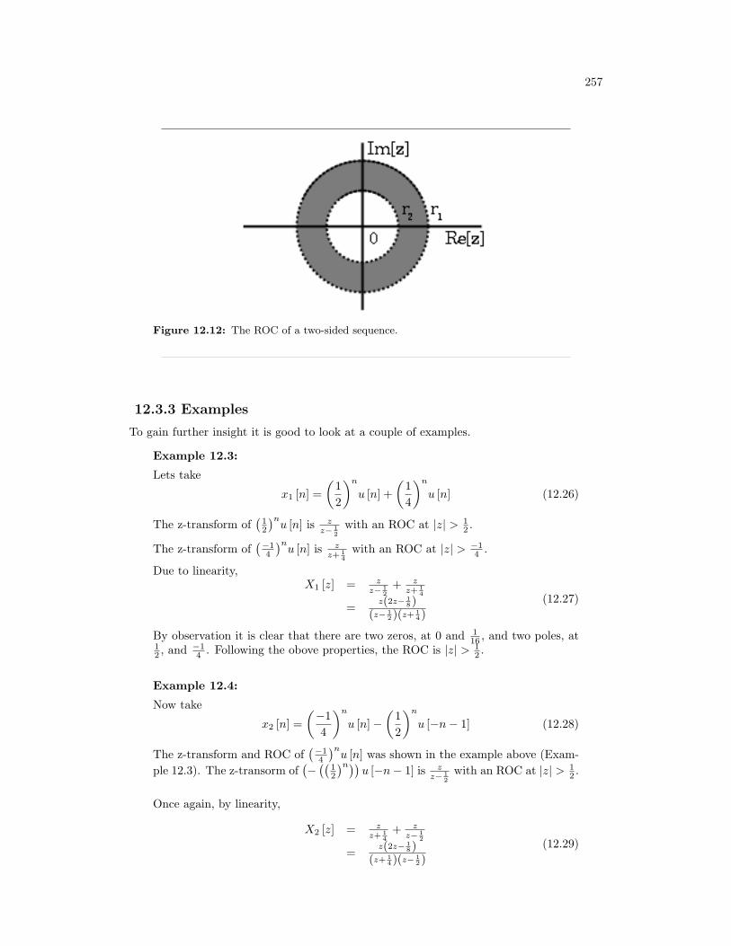
257
Figure 12.12: The ROC of a two-sided sequence.
12.3.3 Examples
To gain further insight it is good to look at a couple of examples.
Example 12.3:
Lets take
x1 [n] =(
12
)n
u [n] +(
14
)n
u [n] (12.26)
The z-transform of(
12
)nu [n] is z
z− 12
with an ROC at |z| > 12 .
The z-transform of(−1
4
)nu [n] is z
z+ 14
with an ROC at |z| > −14 .
Due to linearity,X1 [z] = z
z− 12
+ zz+ 1
4
=z(2z− 1
8 )(z− 1
2 )(z+ 14 )
(12.27)
By observation it is clear that there are two zeros, at 0 and 116 , and two poles, at
12 , and −1
4 . Following the obove properties, the ROC is |z| > 12 .
Example 12.4:
Now take
x2 [n] =(−14
)n
u [n]−(
12
)n
u [−n− 1] (12.28)
The z-transform and ROC of(−1
4
)nu [n] was shown in the example above (Exam-
ple 12.3). The z-transorm of(−((
12
)n))u [−n− 1] is z
z− 12
with an ROC at |z| > 12 .
Once again, by linearity,
X2 [z] = zz+ 1
4+ z
z− 12
=z(2z− 1
8 )(z+ 1
4 )(z− 12 )
(12.29)
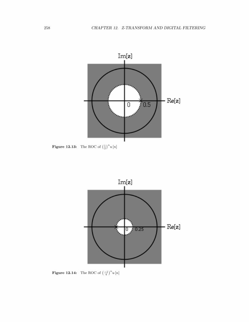
258 CHAPTER 12. Z-TRANSFORM AND DIGITAL FILTERING
Figure 12.13: The ROC of(
12
)nu [n]
Figure 12.14: The ROC of(−1
4
)nu [n]
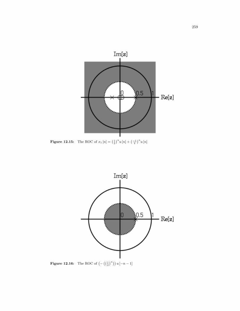
259
Figure 12.15: The ROC of x1 [n] =(
12
)nu [n] +
(−14
)nu [n]
Figure 12.16: The ROC of(−
((12
)n))u [−n− 1]
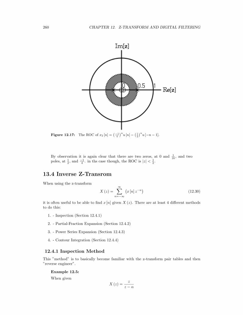
260 CHAPTER 12. Z-TRANSFORM AND DIGITAL FILTERING
Figure 12.17: The ROC of x2 [n] =(−1
4
)nu [n]−
(12
)nu [−n− 1].
By observation it is again clear that there are two zeros, at 0 and 116 , and two
poles, at 12 , and −1
4 . in ths case though, the ROC is |z| < 12 .
13.4 Inverse Z-Transrom
When using the z-transform
X (z) =∞∑
n=−∞
(x [n] z−n
)(12.30)
it is often useful to be able to find x [n] given X (z). There are at least 4 different methodsto do this:
1. - Inspection (Section 12.4.1)
2. - Partial-Fraction Expansion (Section 12.4.2)
3. - Power Series Expansion (Section 12.4.3)
4. - Contour Integration (Section 12.4.4)
12.4.1 Inspection Method
This ”method” is to basically become familiar with the z-transform pair tables and then”reverse engineer”.
Example 12.5:
When givenX (z) =
z
z − α
261
with an ROC of|z| > α
we could determine ”by inspection” that
x [n] = αnu [n]
12.4.2 Partial-Fraction Expansion Method
When dealing with linear time-invariant systems the z-transorm often in the form
X (z) = B(z)A(z)
=∑M
k=0(bkz−k)∑Nk=0(akz−k)
(12.31)
This can also expressed as
X (z) =a0
b0
∏Mk=1
(1− ckz
−1)∏N
k=1 (1− dkz−1)(12.32)
where ck reprisents the nonzero zeros of X (z) and dk reprisents the nonzero poles.If M < N then X (z) can be reprisented as
X (z) =N∑
k=1
(Ak
1− dkz−1
)(12.33)
This form allows for easy inversions of each term of the sum using the inspection method(Section 12.4.1) and the transform table. Thus if the numerator is a polynomial then it isnecessary to use partial-fraction expansion to put X (z) in the above form. If M ≥ N thenX (z) can be expressed as
X (z) =M−N∑r=0
(Brz
−r)
+∑N−1
k=0
(b’kz
−k)∑N
k=0 (akz−k)(12.34)
Example 12.6:
Find the inverse z-transform of
X (z) =1 + 2z−1 + z−2
1 + (−3z−1) + 2z−2
where the ROC is |z| > 2. In this case M = N = 2, so we have to use long divisionto get
X (z) =12
+12 + 7
2z−1
1 + (−3z−1) + 2z−2
Next factor the denominator.
X (z) = 2 +(−1) + 5z−1
(1− 2z−1) (1− z−1)
Now do partial-fraction expansion.
X (z) =12
+A1
1− 2z−1+
A2
1− z−1=
12
+92
1− 2z−1+
−41− z−1
Now each term can be inverted using the inspection method and the z-transformtable. Thus, since the ROC is |z| > 2,
x [n] =12δ [n] +
922nu [n] + (−4u [n])
262 CHAPTER 12. Z-TRANSFORM AND DIGITAL FILTERING
12.4.3 Power Series Expansion Method
When the z-transform is defined as a power series in the form
X (z) =∞∑
n=−∞
(x [n] z−n
)(12.35)
then each term of the sequence x [n] can be determined by looking at the coefficients of therespective power of z−n.
Example 12.7:
Now look at the z-transform of a finite-length sequence .
X (z) = z2(1 + 2z−1
) (1− 1
2z−1) (
1 + z−1)
= z2 + 52z + 1
2 +(−(z−1)) (12.36)
In this case, since there were no poles, we multiplied the factors of X (z). Now, byinspection, it is clear that
x [n] = δ [n+ 2] +52δ [n+ 1] +
12δ [n] + (− (δ [n− 1]))
.
One of the advantages of the power series expansion method is that many functionsencountered in engineering problems have their power series’ tabulated. Thus functionssuch as log, sin, exponent, sinh, etc, can be easily inverted.
Example 12.8:
SupposeX (z) = logn
(1 + αz−1
)Noting that
logn (1 + x) =∞∑
n=1
(−1n+1xn
n
)Then
X (z) =∞∑
n=1
(−1n+1αnz−n
n
)Therefore
=
−1n+1αn
n if n ≥ 10 if n ≤ 0
12.4.4 Contour Integration Method
Without going in to much detail
x [n] =1
2πj
∮r
X (z) zn−1dz (12.37)
where r is a counter-clockwise countour in the ROC of X (z) encirciling the origin of thez-plane. To further expand on this method of finding the inverse requires the knowledge ofcomplex variable theory and thus will not be addressed in this module.
263
13.5 Rational Functions
12.5.1 Introduction
When dealing with operations on polynomials, the term rational function is a simple wayto describe a particular relationship between two polynomials.
rational function : For any two polynomails, A and B, their quotient is calleda rational function.
Example 98:Below is a simple example of a basic rational function, f (x). Note thatthe numerator and denomenator can be polynomials of any order, but therational function is undefined when the denomenator equals zero.
f (x) =x2 − 4
2x2 + x− 3(12.38)
If you have begun to study the Z-transform, you should have noticed by now they areall rational functions. Below we will look at some of the properties of rational functions andhow they can be used to reveal important characteristics about a z-transform, and thus asignal or LTI system.
12.5.2 Properties of Rational Functions
In order to see what makes rational functions special, let us look at some of their basicproperties and characteristics. If you are familiar with rational functions and basic algebraicproperties, skip to the next section (Section 12.5.3) to see how rational functions are usefulwhen dealing with the z-transform.
12.5.2.1 Roots
To understand many of the following characteristics of a rational function, one must beginby finding the roots of the rational function. In order to do this, let us factor both of thepolynomials so that the roots can be easily determined. Like all polynomials, the roots willprovide us with information on many key properties. The function below shows the resultsof factoring the above rational function, Equation 12.38.
f (x) =(x+ 2) (x− 2)(2x+ 3) (x− 1)
(12.39)
Thus, the roots of the rational function are as follows:Roots of the numerator are: −2, 2Roots of the denomenator are: −3, 1
note: In order to understand rational functions, it is essential to know andunderstand the roots that make up the rational function.
12.5.2.2 Discontinuities
Because we are dealing with division of two polynomials, we must be aware of the values ofthe variable that will cause the denominator of our fraction to be zero. When this happens,the rational function becomes undefined, i.e. we have a discontinuity in the function. Be-cause we have already solved for our roots, it is very easy to see when this occurs. Whenthe variable in the denomenator equals any of the roots of the denomenator, the functionbecomes undefined.
264 CHAPTER 12. Z-TRANSFORM AND DIGITAL FILTERING
Example 12.9:
Continuing to look at our rational funtion above, Equation 12.38, we can see thatthe function will have dicontinuites at the following points: x = −3, 1
In respect to the cartesian plane, we say that the discontinuities are the values alongthe x-axis where the function in undefined. These discontinuities often appear as verticalasymptotes on the graph to represent the values where the function is undefined.
12.5.2.3 Domain
Using the roots that we found above, the domain of the rational function can be easilydefined.
domain : The group, or set, of values that are defined by a given function.
Example 100:Using the rational function above, Equation 12.38, the domain can bedefined as any real number x where x does not equal 1 or negative 3.Written out mathematical, we get the following:
x ∈ R |x 6= −3 x 6= 1 (12.40)
12.5.2.4 Intercepts
The x-intercept is defined as the point(s) where f (x), i.e. the output of the rationalfunctions, equals zero. Because we have already found the roots of the equation this processis very simple. From algebra, we know that the output will be zero whenever the numeratorof the rational function is equal to zero. Therefore, the function will have an x-interceptwherever x equals one of the roots of the numerator.
The y-intercept occurs whenever x equals zero. This can be found by setting all thevalues of x equal to zero and solving the rational function.
12.5.3 Rational Functions and the Z-Transform
As we have stated above, all z-transforms can be written as rational functions, which havebecome the most common way of representing the z-transform. Because of this, we can usethe properties above, especially those of the roots, in order to reveal certain characteristicsabout the signal or LTI system described by the z-transform.
Below is the general form of the z-transform written as a rational function:
X (z) =b0 + b1z
−1 + · · ·+ bMz−M
a0 + a1z−1 + · · ·+ aNz−N(12.41)
If you have already looked at the module about Understanding Pole/Zero Plots and theZ-transform, you should see how the roots of the rational function play an important rolein understanding the z-transform. The equation above, Equation 12.41, can be expressed infactored form just as was done for the simple rational function above, see Equation 12.39.Thus, we can easily find the roots of the numerator and denomenator of the z-transform.The following two relationships become apparent:
Relationship of Roots to Poles and Zeros
• - The roots of the numerator in the rational function will be the zeros of the z-transform
• - The roots of the denomenator in the rational function will be the poles of thez-transform
265
12.5.4 Conclusion
Once we have used our knowledge of rational fuctions to find its roots, we can manipulatea z-transform in a number of useful ways. We can apply this knowledge to representing anLTI system graphically through a Pole/Zero Plot, or to analyze and design a digital filterthrough Filter Design from the Z-Transform.
13.6 Difference Equation
12.6.1 Introduction
One of the most important concepts of DSP is to be able to properly represent the in-put/ouput relationship to a given LTI system. A linear constant-coefficient differenceequation (LCCDE) serves as a way to express just this relationship in a discrete-time sys-tem. Writing the sequence of inputs and outputs, which represent the charateristics of theLTI system, as a difference equation help in understanding and manipulating a system.
difference equation : An equation that shows the relationship between con-secutive values of a sequence and the differences among them. They are oftenrearranged as a recursive formula so that a systems output can be computed fromthe input signal and past outputs.
Example 101:
y [n] + 7y [n− 1] + 2y [n− 2] = x [n]− 4x [n− 1] (12.42)
12.6.2 General Formulas from the Difference Equation
As stated briefly in the definition above, a difference equation is a very useful tool in describ-ing and calculating the output of the system described by the formula for a given sample n.The key property of the difference equation is its ability to help easily find the transform,H (z), of a system. In the following two subsections, we will look at the general form of thedifference equation and the general conversion to a z-transform directly from the differenceequation.
12.6.2.1 Difference Equation
The general form of a linear, constant-coefficient difference equation (LCCDE), is shownbelow:
N∑k=0
(aky [n− k]) =M∑
k=0
(bkx [n− k]) (12.43)
We can also write the general form to easily express a recursive output, which looks likethis:
y [n] = −
(N∑
k=1
(aky [n− k])
)+
M∑k=0
(bkx [n− k]) (12.44)
From this equation, note that y [n− k] represents the outputs and x [n− k] represents theinputs. The value of N represents the order of the difference equation and corresponds tothe memory of the system being represented. Because this equation relies on past values ofthe output, in order to compute a numerical solution, certain past outputs, referred to asthe initial conditions , must be known.
266 CHAPTER 12. Z-TRANSFORM AND DIGITAL FILTERING
12.6.2.2 Conversion to Z-Transform
Using the above formula, Equation 12.43, we can easily generalize the transfer function, H (z), for any difference equation. Below are the steps taken to convert any differenceequation into its transfer function, i.e. z-transform. The first step involves taking theFourier Transform of all the terms in Equation 12.43. Then we use the linearity property topull the transform inside the summation and the time-shifting property of the z-transform tochange the time-shifting terms to exponentials. Once this is done, we arrive at the followinequation: a0 = 1.
Y (z) = −
(N∑
k=1
(akY (z) z−k
))+
M∑k=0
(bkX (z) z−k
)(12.45)
H (z) = Y (z)X(z)
=∑M
k=0(bkz−k)1+∑N
k=1(akz−k)
(12.46)
12.6.2.3 Conversion to Frequency Response
Once the z-transform has been calculated from the difference equation, we can go one stepfurther to define the frequency response of the system, or filter, that is being representedby the difference equation.
note: Remember that the reason we are dealing with these formulas is to beable to aid us in filter design. A LCCDE is one of the easiest ways to representFIR filters. By being able to find the frequency response, we will be able to lookat the basic properties of any filter represented by a simple LCCDE.
Below is the general formula for the frequency response of a z-transform. The conversion issimple a matter of taking the z-transform forumula, H (z), and replacing every instance ofz with ejw.
H (w) = H (z) |z,z=ejw
=∑M
k=0(bke−(jwk))∑Nk=0(ake−(jwk))
(12.47)
Once you understand the derivation of this formula, look at the module concerning FilterDesign from the Z-Transform for a look into how all of these ideas of the Z-transform,Difference Equation, and Pole/Zero Plots play a role in filter design.
12.6.3 Example
Example 12.10: Finding Difference Equation
Below is a basic example showing the opposite of the steps above: given a transferfunction one can easily calculate the systems difference equation.
H (z) =(z + 1)2(
z − 12
) (z + 3
4
) (12.48)
Given this transfer function of a time-domain filter, we want to find the differenceequation. To begin with, expand both polynomials and divide them by the highestorder z.
H (z) = (z+1)(z+1)
(z− 12 )(z+ 3
4 )= z2+2z+1
z2+2z+1− 38
= 1+2z−1+z−2
1+ 14 z−1− 3
8 z−2
(12.49)
267
From this transfer function, the coefficients of the two polynomials will be our ak
and bk values found in the general difference equation formula, Equation 12.43.Using these coefficients and the above form of the transfer function, we can easilywrite the difference equation:
x [n] + 2x [n− 1] + x [n− 2] = y [n] +14y [n− 1]− 3
8y [n− 2] (12.50)
In our final step, we can rewrite the difference equation in its more common formshowing the recursive nature of the system.
y [n] = x [n] + 2x [n− 1] + x [n− 2] +−14y [n− 1] +
38y [n− 2] (12.51)
12.6.4 Solving a LCCDE
In order for a linear constant-coefficient difference equation to be useful in analyzing a LTIsystem, we must be able to find the systems output based upon a known input, x (n), anda set of initial conditions. Two common methods exist for solving a LCCDE: the directmethod and the indirect method , the later being based on the z-transform. Below wewill briefly discuss the formulas for solving a LCCDE using each of these methods.
12.6.4.1 Direct Method
The final solution to the output based on the direct method is the sum of two parts, expressedin the following equation:
y (n) = yh (n) + yp (n) (12.52)
The first part, yh (n), is referred to as the homogeneous solution and the second part,yh (n), is referred to as particular solution . The following method is very similar to thatused to solve many differential equations, so if you have taken a differential calculus courseor used differential equations before then this should seem very familiar.
12.6.4.1.1 Homogeneous Solution
We begin by assuming that the input is zero, x (n) = 0. Now we simply need to solve thehomogeneous difference equation:
N∑k=0
(aky [n− k]) = 0 (12.53)
In order to solve this, we will make the assumption that the solution is in the form of anexponential. We will use lambda, λ, to represent our exponential terms. We now have tosolve the following equation:
N∑k=0
(akλ
n−k)
= 0 (12.54)
We can expand this equation out and factor out all of the lambda terms. This will give usa large polynomial in paranthesis, which is referred to as the characteristic polynomial .The roots of this polynomial will be the key to solving the homogeneous equation. If thereare all distinct roots, then the general solution to the equation will be as follows:
yh (n) = C1(λ1)n + C2(λ2)
n + · · ·+ CN (λN )n (12.55)
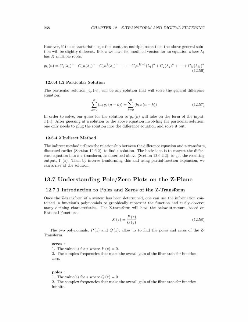
268 CHAPTER 12. Z-TRANSFORM AND DIGITAL FILTERING
However, if the characteristic equation contains multiple roots then the above general solu-tion will be slightly different. Below we have the modified version for an equation where λ1
has K multiple roots:
yh (n) = C1(λ1)n +C1n(λ1)
n +C1n2(λ1)
n + · · ·+C1nK−1(λ1)
n +C2(λ2)n + · · ·+CN (λN )n
(12.56)
12.6.4.1.2 Particular Solution
The particular solution, yp (n), will be any solution that will solve the general differenceequation:
N∑k=0
(akyp (n− k)) =M∑
k=0
(bkx (n− k)) (12.57)
In order to solve, our guess for the solution to yp (n) will take on the form of the input,x (n). After guessing at a solution to the above equation involvling the particular solution,one only needs to plug the solution into the difference equation and solve it out.
12.6.4.2 Indirect Method
The indirect method utilizes the relationship between the difference equation and z-transform,discussed earlier (Section 12.6.2), to find a solution. The basic idea is to convert the differ-ence equation into a z-transform, as described above (Section 12.6.2.2), to get the resultingoutput, Y (z). Then by inverse tranforming this and using partial-fraction expansion, wecan arrive at the solution.
13.7 Understanding Pole/Zero Plots on the Z-Plane
12.7.1 Introduction to Poles and Zeros of the Z-Transform
Once the Z-transform of a system has been determined, one can use the information con-tained in function’s polynomials to graphically represent the function and easily observemany defining characteristics. The Z-transform will have the below structure, based onRational Functions:
X (z) =P (z)Q (z)
(12.58)
The two polynomials, P (z) and Q (z), allow us to find the poles and zeros of the Z-Transform.
zeros :1. The value(s) for z where P (z) = 0.2. The complex frequencies that make the overall gain of the filter transfer functionzero.
poles :1. The value(s) for z where Q (z) = 0.2. The complex frequencies that make the overall gain of the filter transfer functioninfinite.
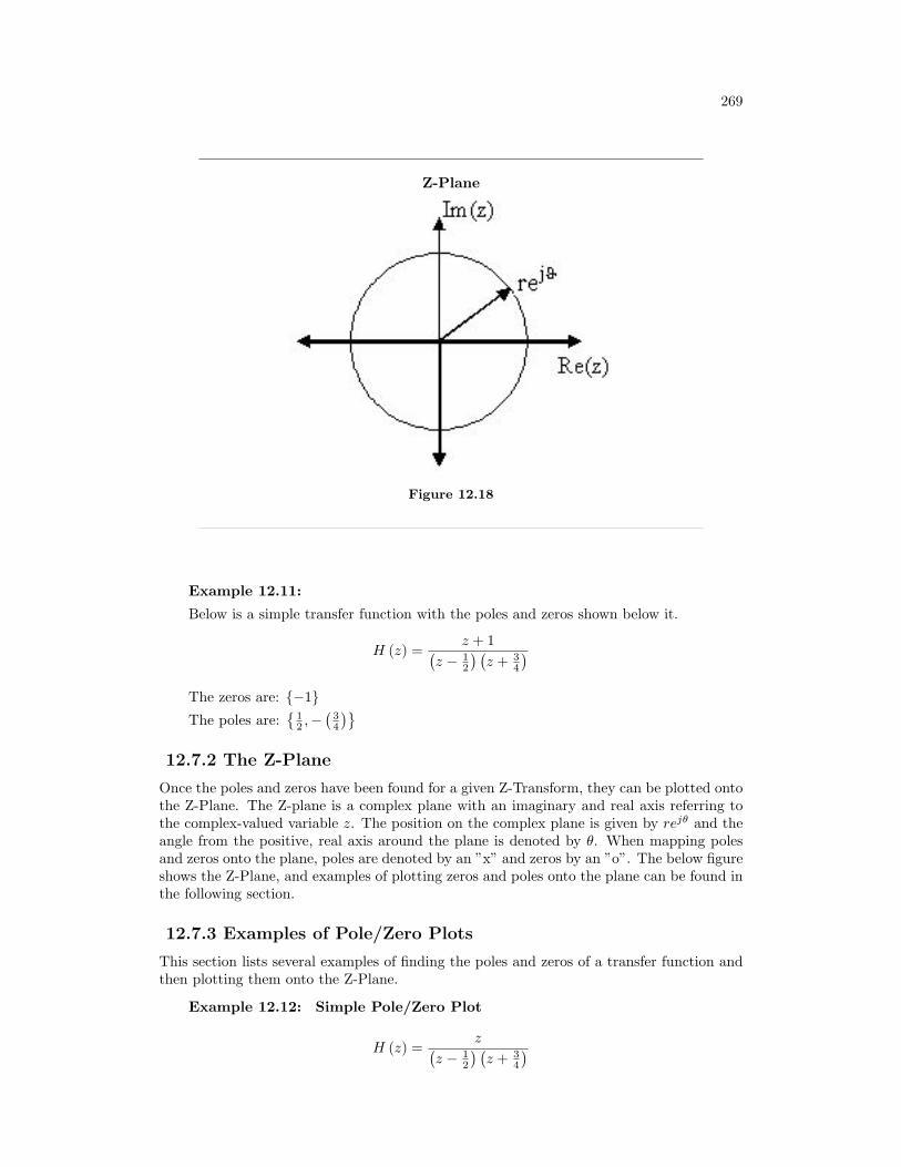
269
Z-Plane
Figure 12.18
Example 12.11:
Below is a simple transfer function with the poles and zeros shown below it.
H (z) =z + 1(
z − 12
) (z + 3
4
)The zeros are: −1The poles are:
12 ,−
(34
)12.7.2 The Z-Plane
Once the poles and zeros have been found for a given Z-Transform, they can be plotted ontothe Z-Plane. The Z-plane is a complex plane with an imaginary and real axis referring tothe complex-valued variable z. The position on the complex plane is given by rejθ and theangle from the positive, real axis around the plane is denoted by θ. When mapping polesand zeros onto the plane, poles are denoted by an ”x” and zeros by an ”o”. The below figureshows the Z-Plane, and examples of plotting zeros and poles onto the plane can be found inthe following section.
12.7.3 Examples of Pole/Zero Plots
This section lists several examples of finding the poles and zeros of a transfer function andthen plotting them onto the Z-Plane.
Example 12.12: Simple Pole/Zero Plot
H (z) =z(
z − 12
) (z + 3
4
)
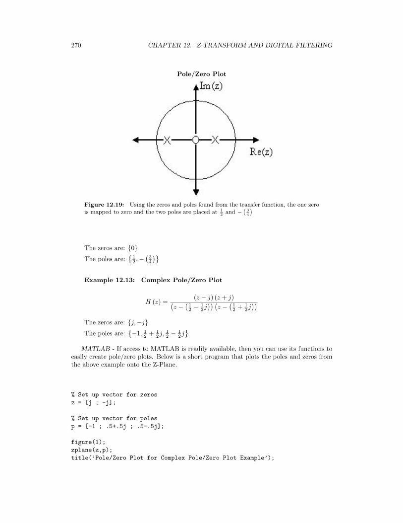
270 CHAPTER 12. Z-TRANSFORM AND DIGITAL FILTERING
Pole/Zero Plot
Figure 12.19: Using the zeros and poles found from the transfer function, the one zerois mapped to zero and the two poles are placed at 1
2and −
(34
)
The zeros are: 0The poles are:
12 ,−
(34
)Example 12.13: Complex Pole/Zero Plot
H (z) =(z − j) (z + j)(
z −(
12 −
12j)) (
z −(
12 + 1
2j))
The zeros are: j,−jThe poles are:
−1, 1
2 + 12j,
12 −
12j
MATLAB - If access to MATLAB is readily available, then you can use its functions toeasily create pole/zero plots. Below is a short program that plots the poles and zeros fromthe above example onto the Z-Plane.
% Set up vector for zerosz = [j ; -j];
% Set up vector for polesp = [-1 ; .5+.5j ; .5-.5j];
figure(1);zplane(z,p);title(’Pole/Zero Plot for Complex Pole/Zero Plot Example’);
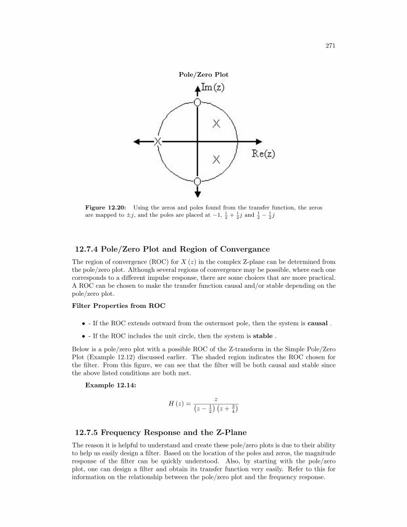
271
Pole/Zero Plot
Figure 12.20: Using the zeros and poles found from the transfer function, the zerosare mapped to ±j, and the poles are placed at −1, 1
2+ 1
2j and 1
2− 1
2j
12.7.4 Pole/Zero Plot and Region of Convergance
The region of convergence (ROC) for X (z) in the complex Z-plane can be determined fromthe pole/zero plot. Although several regions of convergence may be possible, where each onecorresponds to a different impulse response, there are some choices that are more practical.A ROC can be chosen to make the transfer function causal and/or stable depending on thepole/zero plot.
Filter Properties from ROC
• - If the ROC extends outward from the outermost pole, then the system is causal .
• - If the ROC includes the unit circle, then the system is stable .
Below is a pole/zero plot with a possible ROC of the Z-transform in the Simple Pole/ZeroPlot (Example 12.12) discussed earlier. The shaded region indicates the ROC chosen forthe filter. From this figure, we can see that the filter will be both causal and stable sincethe above listed conditions are both met.
Example 12.14:
H (z) =z(
z − 12
) (z + 3
4
)12.7.5 Frequency Response and the Z-Plane
The reason it is helpful to understand and create these pole/zero plots is due to their abilityto help us easily design a filter. Based on the location of the poles and zeros, the magnituderesponse of the filter can be quickly understood. Also, by starting with the pole/zeroplot, one can design a filter and obtain its transfer function very easily. Refer to this forinformation on the relationship between the pole/zero plot and the frequency response.
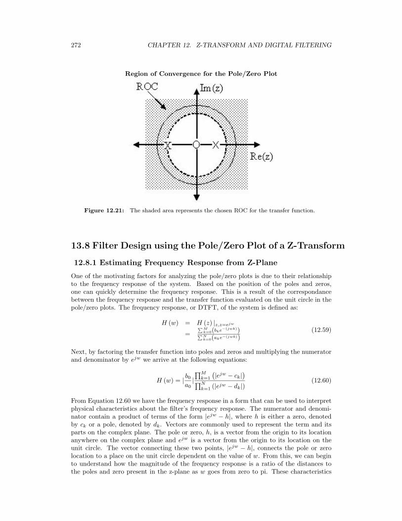
272 CHAPTER 12. Z-TRANSFORM AND DIGITAL FILTERING
Region of Convergence for the Pole/Zero Plot
Figure 12.21: The shaded area represents the chosen ROC for the transfer function.
13.8 Filter Design using the Pole/Zero Plot of a Z-Transform
12.8.1 Estimating Frequency Response from Z-Plane
One of the motivating factors for analyzing the pole/zero plots is due to their relationshipto the frequency response of the system. Based on the position of the poles and zeros,one can quickly determine the frequency response. This is a result of the correspondancebetween the frequency response and the transfer function evaluated on the unit circle in thepole/zero plots. The frequency response, or DTFT, of the system is defined as:
H (w) = H (z) |z,z=ejw
=∑M
k=0(bke−(jwk))∑Nk=0(ake−(jwk))
(12.59)
Next, by factoring the transfer function into poles and zeros and multiplying the numeratorand denominator by ejw we arrive at the following equations:
H (w) = | b0a0|∏M
k=1
(|ejw − ck|
)∏Nk=1 (|ejw − dk|)
(12.60)
From Equation 12.60 we have the frequency response in a form that can be used to interpretphysical characteristics about the filter’s frequency response. The numerator and denomi-nator contain a product of terms of the form |ejw − h|, where h is either a zero, denotedby ck or a pole, denoted by dk. Vectors are commonly used to represent the term and itsparts on the complex plane. The pole or zero, h, is a vector from the origin to its locationanywhere on the complex plane and ejw is a vector from the origin to its location on theunit circle. The vector connecting these two points, |ejw − h|, connects the pole or zerolocation to a place on the unit circle dependent on the value of w. From this, we can beginto understand how the magnitude of the frequency response is a ratio of the distances tothe poles and zero present in the z-plane as w goes from zero to pi. These characteristics
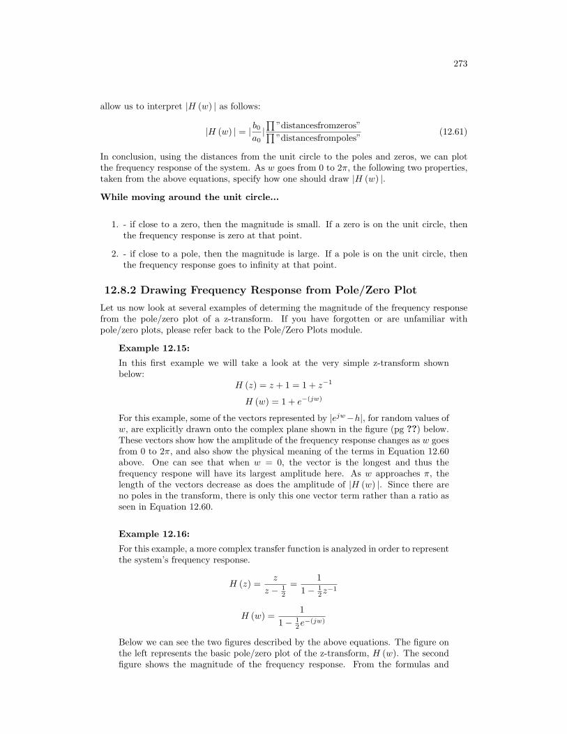
273
allow us to interpret |H (w) | as follows:
|H (w) | = | b0a0|∏
”distancesfromzeros”∏”distancesfrompoles”
(12.61)
In conclusion, using the distances from the unit circle to the poles and zeros, we can plotthe frequency response of the system. As w goes from 0 to 2π, the following two properties,taken from the above equations, specify how one should draw |H (w) |.
While moving around the unit circle...
1. - if close to a zero, then the magnitude is small. If a zero is on the unit circle, thenthe frequency response is zero at that point.
2. - if close to a pole, then the magnitude is large. If a pole is on the unit circle, thenthe frequency response goes to infinity at that point.
12.8.2 Drawing Frequency Response from Pole/Zero Plot
Let us now look at several examples of determing the magnitude of the frequency responsefrom the pole/zero plot of a z-transform. If you have forgotten or are unfamiliar withpole/zero plots, please refer back to the Pole/Zero Plots module.
Example 12.15:
In this first example we will take a look at the very simple z-transform shownbelow:
H (z) = z + 1 = 1 + z−1
H (w) = 1 + e−(jw)
For this example, some of the vectors represented by |ejw−h|, for random values ofw, are explicitly drawn onto the complex plane shown in the figure (pg ??) below.These vectors show how the amplitude of the frequency response changes as w goesfrom 0 to 2π, and also show the physical meaning of the terms in Equation 12.60above. One can see that when w = 0, the vector is the longest and thus thefrequency respone will have its largest amplitude here. As w approaches π, thelength of the vectors decrease as does the amplitude of |H (w) |. Since there areno poles in the transform, there is only this one vector term rather than a ratio asseen in Equation 12.60.
Example 12.16:
For this example, a more complex transfer function is analyzed in order to representthe system’s frequency response.
H (z) =z
z − 12
=1
1− 12z−1
H (w) =1
1− 12e−(jw)
Below we can see the two figures described by the above equations. The figure onthe left represents the basic pole/zero plot of the z-transform, H (w). The secondfigure shows the magnitude of the frequency response. From the formulas and
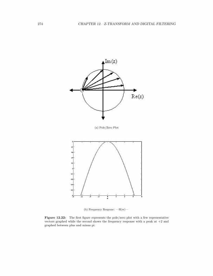
274 CHAPTER 12. Z-TRANSFORM AND DIGITAL FILTERING
(a) Pole/Zero Plot
(b) Frequency Respone: —H(w)—
Figure 12.22: The first figure represents the pole/zero plot with a few representativevectors graphed while the second shows the frequency response with a peak at +2 andgraphed between plus and minus pi.
275
statements in the previous section, we can see that when w = 0 the frequency willpeak since it is at this value of w that the pole is closest to the unit circle. Theratio from Equation 12.60 helps us see the mathematics behind this conclusion andthe relationship between the distances from the unit circle and the poles and zeros.As w moves from 0 to π, we see how the zero begins to mask the effects of the poleand thus force the frequency response closer to 0.
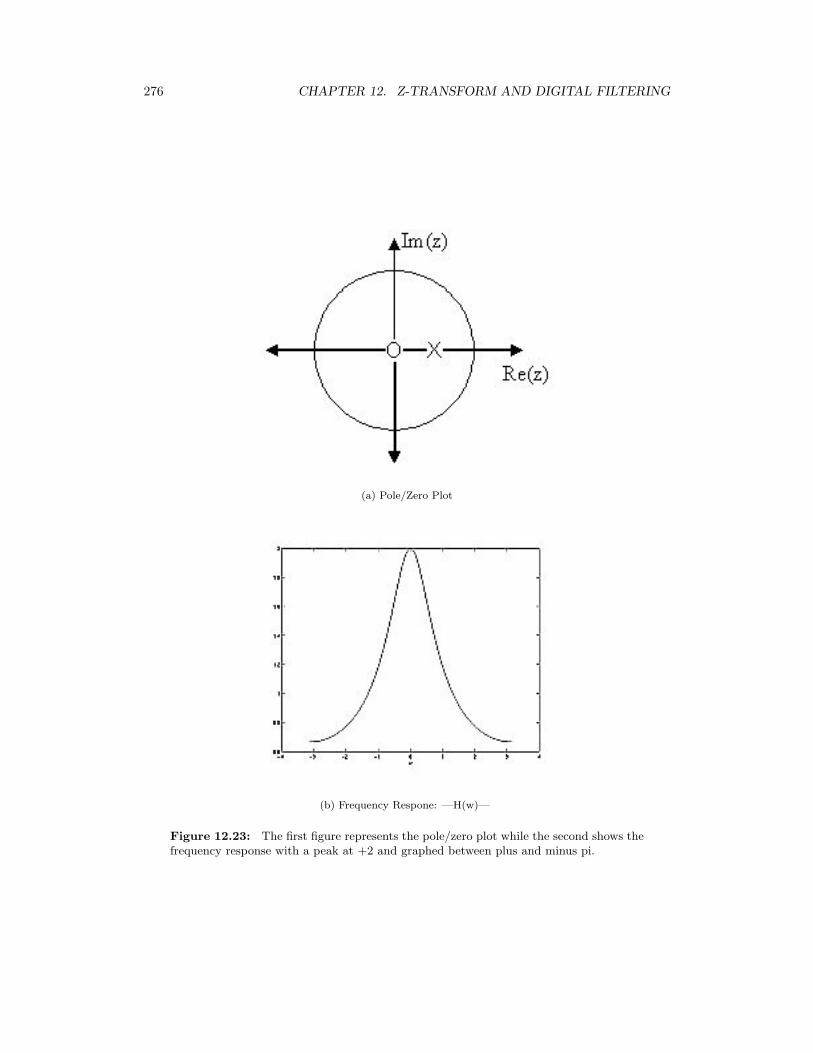
276 CHAPTER 12. Z-TRANSFORM AND DIGITAL FILTERING
(a) Pole/Zero Plot
(b) Frequency Respone: —H(w)—
Figure 12.23: The first figure represents the pole/zero plot while the second shows thefrequency response with a peak at +2 and graphed between plus and minus pi.

Chapter 13
Homework Sets
14.1 Homework #1
due date: Noon, Thursday, September 5, 2002
13.1.1 Assignment 1
Homework, tests, and solutions from previous offerings of this course are off limits, underthe honor code.
13.1.1.1 Problem 1
Form a study group of 3-4 members. With your group, discuss and synthesize the majorthemes of this week of lectures. Turn in a one page summary of your discussion. You needturn in only one summary per group, but include the names of all group members. Pleasedo not write up just a ”table of contents.”
13.1.1.2 Problem 2
Construct a WWW page (with your picture) and email Mike Wakin ([email protected]) yourname (as you want it to appear on the class web page) and the URL. If you need assistancesetting up your page or taking/scanning a picture (both are easy!), ask your classmates.
13.1.1.3 Problem 3: Learning Styles
Follow this learning styles link1 (also found on the Elec 301 web page2) and learn about thebasics of learning styles. Write a short summary of what you learned. Also, complete the“Index of learning styles” self-scoring test on the web and bring your results to class.
13.1.1.4 Problem 4
Make sure you know the material in Lathi, Chapter B, Sections 1-4, 6.1, 6.2, 7. Specifically,be sure to review topics such as:
• - complex arithmetic (adding, multiplying, powers)
• - finding (complex) roots of polynomials
1http://www2.ncsu.edu/unity/lockers/users/f/felder/public/Learning Styles.html2http://www-dsp.rice.edu/courses/elec301/
277
278 CHAPTER 13. HOMEWORK SETS
• - complex plane and plotting roots
• - vectors (adding, inner products)
13.1.1.5 Problem 5: Complex Number Applet
Reacquaint yourself with complex numbers by going to the course applets web page3 andclicking on the Complex Numbers applet (may take a few seconds to load).
(a) Change the default add function to exponential (exp). Click on the complex planeto get a blue arrow, which is your complex number z. Click again anywhere on the complexplane to get a yellow arrow, which is equal to ez. Now drag the tip of the blue arrow alongthe unit circle on with |z| = 1 (smaller circle). For which values of z on the unit circle doesez also lie on the unit circle? Why?
(b) Experiment with the functions absolute (abs), real part (re), and imaginary part(im) and report your findings.
13.1.1.6 Problem 6: Complex Arithmetic
Reduce the following to the cartesian form, a+ jb. Do not use your calculator!
(a)(−1−j√
2
)20
(b) 1+2j3+4j
(c) 1+√
3j√3−j
(d)√j
(e) jj
13.1.1.7 Problem 7: Roots of Polynomials
Find the roots of each of the following polynomials (show your work). Use MATLAB tocheck your answer with the roots command and to plot the roots in the complex plane.Mark the root locations with an ’o’. Put all of the roots on the same plot and identify thecorresponding polynomial (a, b, etc...).
(a) z2 − 4z(b) z2 − 4z + 4(c) z2 − 4z + 8(d) z2 + 8(e) z2 + 4z + 8(f) 2z2 + 4z + 8
13.1.1.8 Problem 8: Nth Roots of Unity
ej2πN is called an Nth Root of Unity .(a) Why?(b) Let z = e
j2π7 . Draw
z, z2, . . . , z7
in the complex plane.
(c) Let z = ej4π7 . Draw
z, z2, . . . , z7
in the complex plane.
3http://www.dsp.rice.edu/courses/elec301/applets.shtml
279
13.1.1.9 Problem 9: Writing Vectors in Terms of Other Vectors
A pair of vectors u ∈ C2 and v ∈ C2 are called linearly independent if
αu+ βv = 0 if and only if α = β = 0
It is a fact that we can write any vector in C2 as a weighted sum (or linear combination) of any two linearly independent vectors, where the weights α and β are complex-valued.
(a) Write(
3 + 4j6 + 2j
)as a linear combination of
(12
)and
(−53
). That is, find α
and β such that (3 + 4j6 + 2j
)= α
(12
)+ β
(−53
)(b) More generally, write x =
(x1
x2
)as a linear combination of
(12
)and
(−53
).
We will denote the answer for a given x as α (x) and β (x).(c) Write the answer to (a) in matrix form, i.e. find a 2×2 matrix A such that
A
(x1
x2
)=(α (x)β (x)
)(d) Repeat (b) and (c) for a general set of linearly independent vectors u and v.
13.1.1.10 Problem 10: Fun with Fractals
A Julia set J is obtained by characterizing points in the complex plane. Specifically, letf (x) = x2 + µ with µ complex, and define
g0 (x) = x
g1 (x) = f (g0 (x)) = f (x)
g2 (x) = f (g1 (x)) = f (f (x))
...
gn (x) = f (gn−1 (x))
Then for each x in the complex plane, we say x ∈ J if the sequence
|g0 (x) |, |g1 (x) |, |g2 (x) |, . . .
does not tend to infinity. Notice that if x ∈ J , then each element of the sequence g0 (x) , g1 (x) , g2 (x) , . . . also belongs to J .
For most values of µ, the boundary of a Julia set is a fractal curve - it contains ”jagged”detail no matter how far you zoom in on it. The well-known Mandelbrot set contains allvalues of µ for which the corresponding Julia set is connected.
(a) Let µ = −1. Is x = 1 in J?(b) Let µ = 0. What conditions on x ensure that x belongs to J?(c) Create an approximate picture of a Julia set in MATLAB. The easiest way is to
create a matrix of complex numbers, decide for each number whether it belongs to J , andplot the results using the imagesc command. To determine whether a number belongs toJ , it is helpful to define a limit N on the number of iterations of g. For a given x, if themagnitude |gn (x) | remains below some threshold M for all 0 ≤ n ≤ N , we say that xbelongs to J . The code below will help you get started:
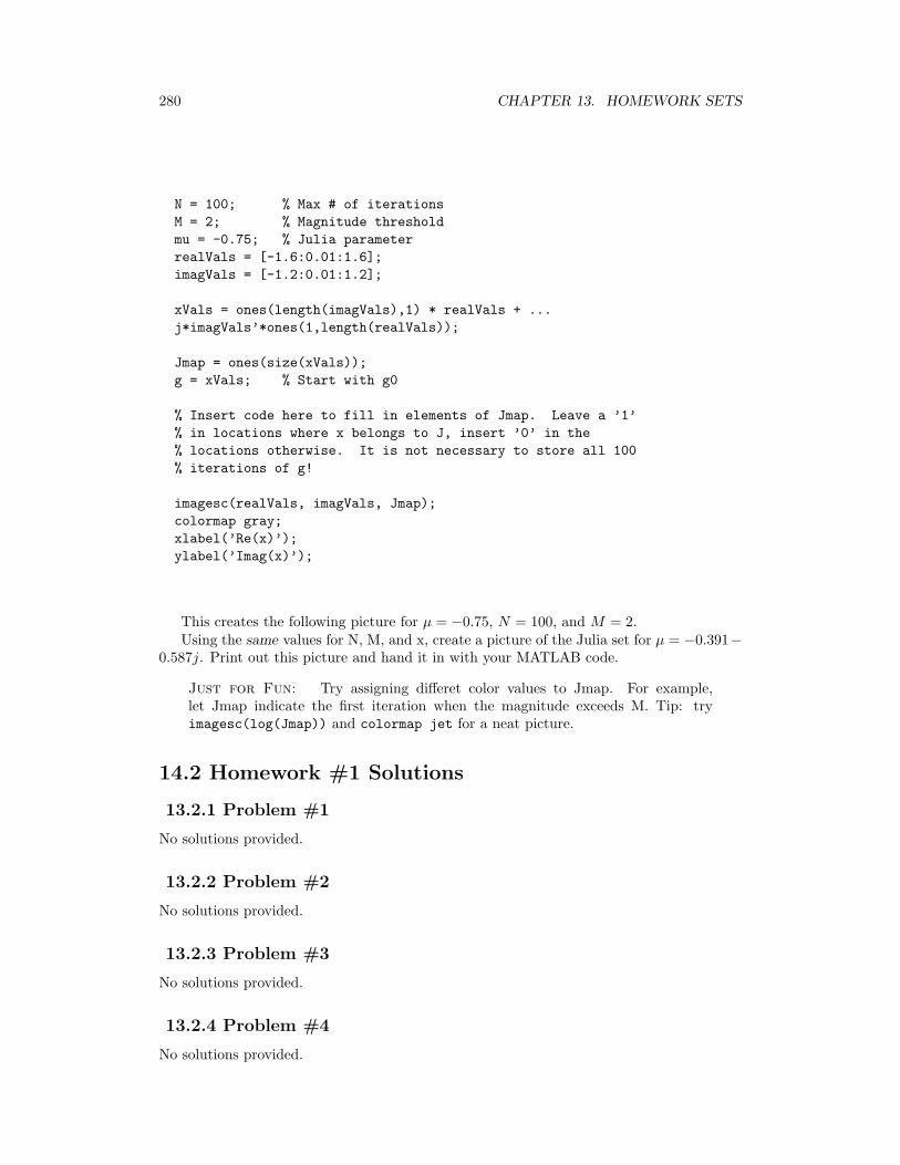
280 CHAPTER 13. HOMEWORK SETS
N = 100; % Max # of iterationsM = 2; % Magnitude thresholdmu = -0.75; % Julia parameterrealVals = [-1.6:0.01:1.6];imagVals = [-1.2:0.01:1.2];
xVals = ones(length(imagVals),1) * realVals + ...j*imagVals’*ones(1,length(realVals));
Jmap = ones(size(xVals));g = xVals; % Start with g0
% Insert code here to fill in elements of Jmap. Leave a ’1’% in locations where x belongs to J, insert ’0’ in the% locations otherwise. It is not necessary to store all 100% iterations of g!
imagesc(realVals, imagVals, Jmap);colormap gray;xlabel(’Re(x)’);ylabel(’Imag(x)’);
This creates the following picture for µ = −0.75, N = 100, and M = 2.Using the same values for N, M, and x, create a picture of the Julia set for µ = −0.391−
0.587j. Print out this picture and hand it in with your MATLAB code.
Just for Fun: Try assigning differet color values to Jmap. For example,let Jmap indicate the first iteration when the magnitude exceeds M. Tip: tryimagesc(log(Jmap)) and colormap jet for a neat picture.
14.2 Homework #1 Solutions
13.2.1 Problem #1
No solutions provided.
13.2.2 Problem #2
No solutions provided.
13.2.3 Problem #3
No solutions provided.
13.2.4 Problem #4
No solutions provided.
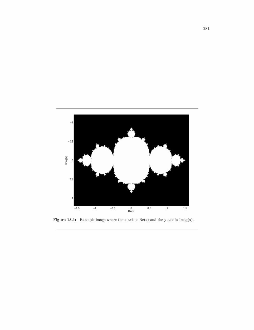
281
Figure 13.1: Example image where the x-axis is Re(x) and the y-axis is Imag(x).
282 CHAPTER 13. HOMEWORK SETS
13.2.5 Problem #5
13.2.5.1 Part (a)
ez lies on the unit circle for z = ±j. When z = ±j,
ez = e±j = cos (±1) + jsin (±1)
e±j =(cos2 (±1) + sin2 (±1)
) 12
= 1(13.1)
which gives us the unit circle!Think of it this way: for z = σ + jθ, you want a σ = 0 so that eσ+jθ reduces as
eσ+jθ = eσejθ = e0ejθ = ejθ
We know by Euler’s formula (Section 2.6.2) that
ejθ = cos (θ) + jsin (θ)
The magnitude of this is given by sin2 (θ) + cos2 (θ), which is 1 (which implies that ejθ ison the unit circle).
So, we know we want to pick a z = Ajθ that is on the unit circle (from the problemstatement), so we have to choose A = ±1 to get unit magnitude.
13.2.5.2 Part (b)
• - abs gives magnitude of complex number
• - re gives real part of complex number
• - im gives imaginary part of complex number
13.2.6 Problem #6
13.2.6.1 Part (a)(−1− j√
2
)20
=
(√2e
5π4
√2
)20
=(e
5π4
)20
= ej25π = ejπ = −1
13.2.6.2 Part (b)
1 + 2j3 + 4j
=(
1 + 2j3 + 4j
)(3− 4j3− 4j
)=
3 + 6j − (4j + 8)9 + 16
=11 + 2j
25=
1125
+225j
13.2.6.3 Part (c)
1 +√
3j√3− j
=2ej π
3
2ej−π6
= ej π2 = j
13.2.6.4 Part (d)√j =
(ej π
2) 1
2 = ej π4 = cos
(π4
)+ jsin
(π4
)=√
22
+√
22j
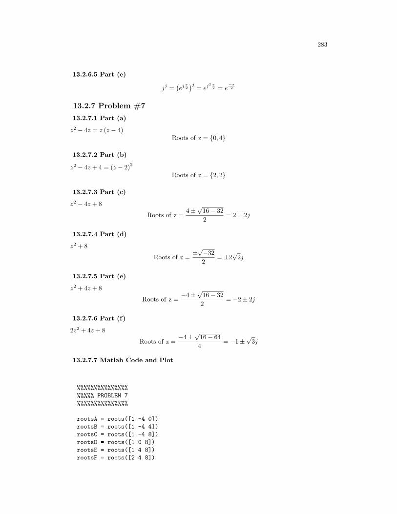
283
13.2.6.5 Part (e)
jj =(ej π
2)j
= ej2 π2 = e
−π2
13.2.7 Problem #7
13.2.7.1 Part (a)
z2 − 4z = z (z − 4)Roots of z = 0, 4
13.2.7.2 Part (b)
z2 − 4z + 4 = (z − 2)2
Roots of z = 2, 2
13.2.7.3 Part (c)
z2 − 4z + 8
Roots of z =4±
√16− 322
= 2± 2j
13.2.7.4 Part (d)
z2 + 8
Roots of z =±√−322
= ±2√
2j
13.2.7.5 Part (e)
z2 + 4z + 8
Roots of z =−4±
√16− 322
= −2± 2j
13.2.7.6 Part (f)
2z2 + 4z + 8
Roots of z =−4±
√16− 644
= −1±√
3j
13.2.7.7 Matlab Code and Plot
%%%%%%%%%%%%%%%%%%%% PROBLEM 7%%%%%%%%%%%%%%%
rootsA = roots([1 -4 0])rootsB = roots([1 -4 4])rootsC = roots([1 -4 8])rootsD = roots([1 0 8])rootsE = roots([1 4 8])rootsF = roots([2 4 8])
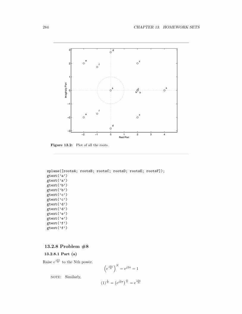
284 CHAPTER 13. HOMEWORK SETS
Figure 13.2: Plot of all the roots.
zplane([rootsA; rootsB; rootsC; rootsD; rootsE; rootsF]);gtext(’a’)gtext(’a’)gtext(’b’)gtext(’b’)gtext(’c’)gtext(’c’)gtext(’d’)gtext(’d’)gtext(’e’)gtext(’e’)gtext(’f’)gtext(’f’)
13.2.8 Problem #8
13.2.8.1 Part (a)
Raise ej2πN to the Nth power. (
ej2πN
)N
= ej2π = 1
note: Similarly,(1)
1N =
(ej2π
) 1N = e
j2πN
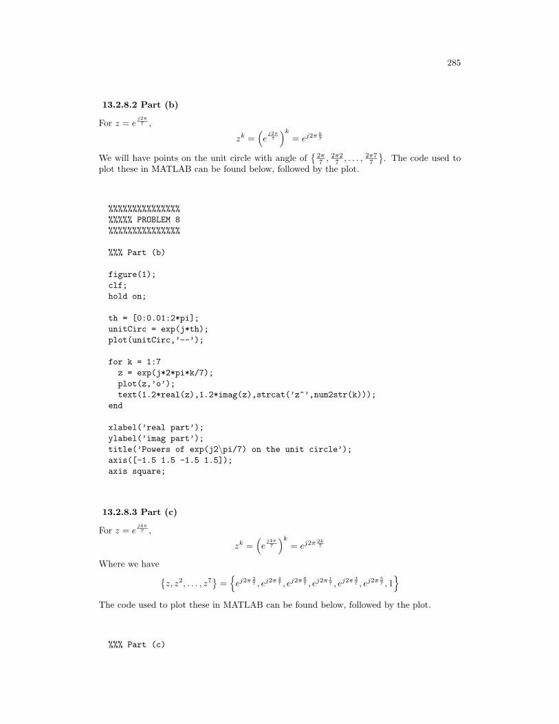
285
13.2.8.2 Part (b)
For z = ej2π7 ,
zk =(e
j2π7
)k
= ej2π k7
We will have points on the unit circle with angle of
2π7 ,
2π27 , . . . , 2π7
7
. The code used to
plot these in MATLAB can be found below, followed by the plot.
%%%%%%%%%%%%%%%%%%%% PROBLEM 8%%%%%%%%%%%%%%%
%%% Part (b)
figure(1);clf;hold on;
th = [0:0.01:2*pi];unitCirc = exp(j*th);plot(unitCirc,’--’);
for k = 1:7z = exp(j*2*pi*k/7);plot(z,’o’);text(1.2*real(z),1.2*imag(z),strcat(’z^’,num2str(k)));
end
xlabel(’real part’);ylabel(’imag part’);title(’Powers of exp(j2\pi/7) on the unit circle’);axis([-1.5 1.5 -1.5 1.5]);axis square;
13.2.8.3 Part (c)
For z = ej4π7 ,
zk =(e
j4π7
)k
= ej2π 2k7
Where we havez, z2, . . . , z7
=ej2π 2
7 , ej2π 47 , ej2π 6
7 , ej2π 17 , ej2π 3
7 , ej2π 57 , 1
The code used to plot these in MATLAB can be found below, followed by the plot.
%%% Part (c)
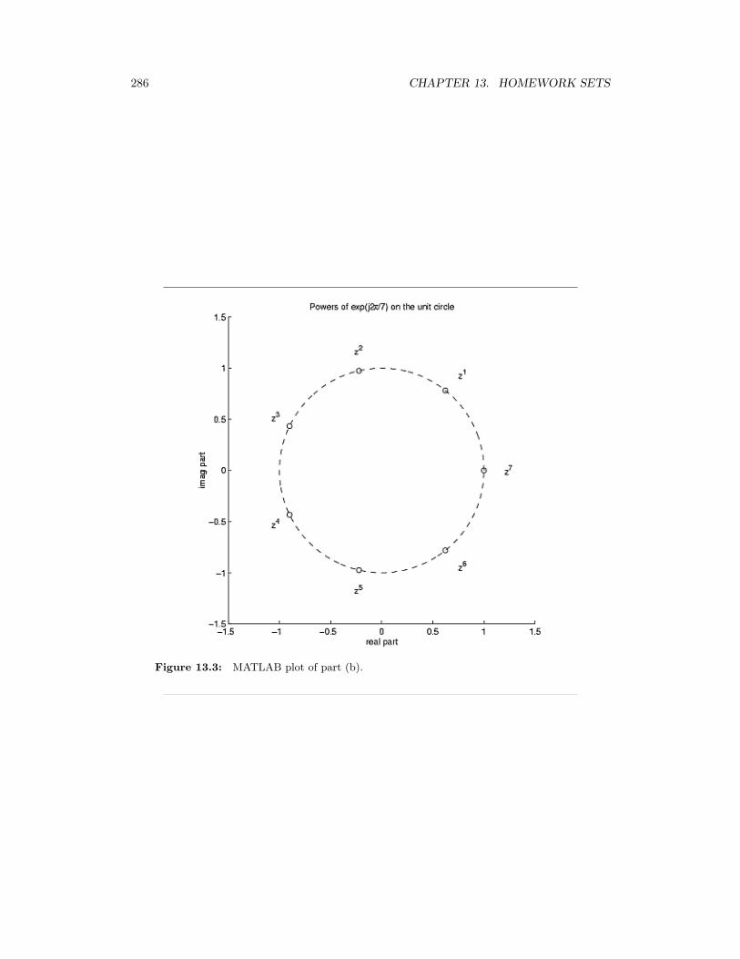
286 CHAPTER 13. HOMEWORK SETS
Figure 13.3: MATLAB plot of part (b).
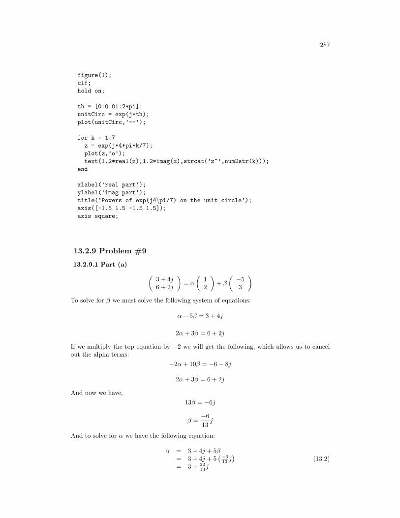
287
figure(1);clf;hold on;
th = [0:0.01:2*pi];unitCirc = exp(j*th);plot(unitCirc,’--’);
for k = 1:7z = exp(j*4*pi*k/7);plot(z,’o’);text(1.2*real(z),1.2*imag(z),strcat(’z^’,num2str(k)));
end
xlabel(’real part’);ylabel(’imag part’);title(’Powers of exp(j4\pi/7) on the unit circle’);axis([-1.5 1.5 -1.5 1.5]);axis square;
13.2.9 Problem #9
13.2.9.1 Part (a) (3 + 4j6 + 2j
)= α
(12
)+ β
(−53
)To solve for β we must solve the following system of equations:
α− 5β = 3 + 4j
2α+ 3β = 6 + 2j
If we multiply the top equation by −2 we will get the following, which allows us to cancelout the alpha terms:
−2α+ 10β = −6− 8j
2α+ 3β = 6 + 2j
And now we have,13β = −6j
β =−613j
And to solve for α we have the following equation:
α = 3 + 4j + 5β= 3 + 4j + 5
(−613 j)
= 3 + 2213j
(13.2)
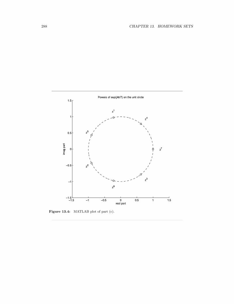
288 CHAPTER 13. HOMEWORK SETS
Figure 13.4: MATLAB plot of part (c).
289
13.2.9.2 Part (b) (x1
x2
)= α
(12
)+ β
(−53
)x1 = α− 5β
x2 = 2α+ 3β
Solving for α and β we get:
α (x) =3x1 + 5x2
13
β (x) =−2x1 + x2
13
13.2.9.3 Part (c) (α (x)β (x)
)=(
313
513−2
13113
)(x1
x2
)13.2.9.4 Part (d)
Write u =(u1
u2
)and v =
(v1v2
). Then solve(
x1
x2
)= α
(u1
u2
)+ β
(v1v2
)which corresponds to the system of equations
x1 = αu1 + βv1
x2 = αu2 + βv2
Solving for α and β we get
α (x) =v2x1 − v1x2
u1v2 − u2v1
β (x) =u2x1 − u1x2
v1u2 − u1v2For the matrix A we get
A =1
u1v2 − u2v1
(v2 −v1
−u2 u1
)13.2.10 Problem #10
13.2.10.1 Part (a)
If u = −1, then f (x) = x2 − 1. Examine the sequence g0 (x) , g1 (x) , . . . :
g0 (x) = 1
g1 (x) = 12 − 1 = 0
g2 (x) = 02 − 1 = −1
g3 (x) = (−1)2 − 1 = 0
g4 (x) = 02 − 1 = −1...
The magnitude sequence remains bounded so x = 1 belongs to J .
290 CHAPTER 13. HOMEWORK SETS
13.2.10.2 Part (b)
If u = 0, then f (x) = x2. So we have
g0 (x) = x
g1 (x) = x2
g2 (x) =(x2)2
= x4
...
gn (x) =(x2)n
= x2n
Writing x = rejθ, we have gn (x) = x2n = r2nejθ2n, and so we have
|gn (x) | = r2n
The magnitude sequence blows up if and only if r > 1. Thus x belongs to J if and only if|x| ≤ 1. So, J corresponds to the unit disk.
13.2.10.3 Part (c)
%%%%%%%%%%%%%%%%%%%%% PROBLEM 10%%%%%%%%%%%%%%%%
%%% Part (c) - solution code
N = 100; % Max # of iterationsM = 2; % Magnitude threshold
mu = -0.391 - 0.587*j; % Julia parameterrealVals = [-1.6:0.01:1.6];imagVals = [-1.2:0.01:1.2];xVals = ones(length(imagVals),1)*realVals + ...j*imagVals’*ones(1,length(realVals));Jmap = ones(size(xVals));g = xVals; % Start with g0
for n = 1:Ng = g.^2 + mu;big = (abs(g) > M);Jmap = Jmap.*(1-big);end
imagesc(realVals,imagVals,Jmap); colormap gray;xlabel(’Re(x)’); ylabel(’Imag(x)’);
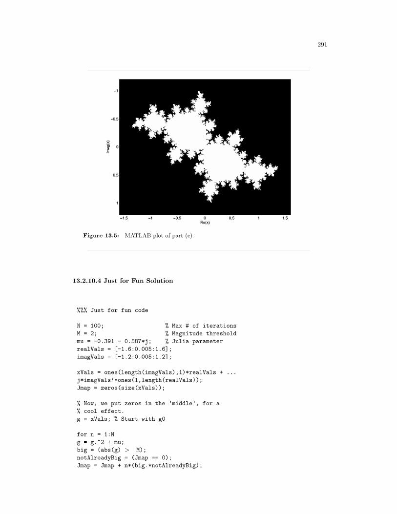
291
Figure 13.5: MATLAB plot of part (c).
13.2.10.4 Just for Fun Solution
%%% Just for fun code
N = 100; % Max # of iterationsM = 2; % Magnitude thresholdmu = -0.391 - 0.587*j; % Julia parameterrealVals = [-1.6:0.005:1.6];imagVals = [-1.2:0.005:1.2];
xVals = ones(length(imagVals),1)*realVals + ...j*imagVals’*ones(1,length(realVals));Jmap = zeros(size(xVals));
% Now, we put zeros in the ’middle’, for a% cool effect.g = xVals; % Start with g0
for n = 1:Ng = g.^2 + mu;big = (abs(g) > M);notAlreadyBig = (Jmap == 0);Jmap = Jmap + n*(big.*notAlreadyBig);
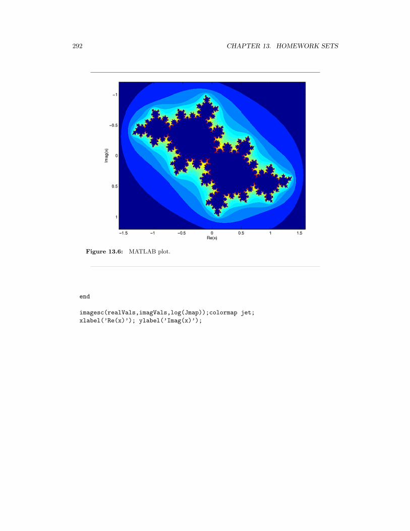
292 CHAPTER 13. HOMEWORK SETS
Figure 13.6: MATLAB plot.
end
imagesc(realVals,imagVals,log(Jmap));colormap jet;xlabel(’Re(x)’); ylabel(’Imag(x)’);
293
Index of Keywords andTermsKeywords are listed by the sectionwith that keyword (page numbers arein parentheses). Keywords do not nec-essarily appear in the text of the page.They are merely associated with thatsection. Ex. apples, § 1.1 (1) Termsare referenced by the page they appearon. Ex. apples, 1
” ”standard basis”, 69
A alias, § 11.5(223), § 11.6(227)aliasing, § 8.2(154), § 11.5(223), 224,§ 11.6(227)almost everywhere, § 6.11(108)alphabet, § 3.4(23), 26analog, § 3.3(14), 17, 23, § 10.6(200),§ 10.7(202)analog signal, § 2.1(3)analysis, 88anitcausal, 17Anti-Aliasing, § 11.6(227)anticausal, § 3.3(14)aperiodic, § 3.3(14)approximation, § 7.13(151)
B bandlimited, 213, § 11.2(215)baraniuk, § 1(1), § 14.2(280)bases, § 7.7(131)basis, § 3.6(30), § 5.1(65), 68, 68, 69,§ 5.4(76), § 7.7(131), § 7.8(135), 135,§ 7.9(139), § 7.10(140), § 7.11(143),§ 8.2(154), 160, § 8.3(163), 219basis matrix, § 7.8(135), 136best approximates, 151BIBO, § 3.1(7), § 3.9(40)bilateral Laplace transform pair, 235bilateral z-transform, 247bounded input bounded output,§ 3.9(40)bounded input-bounded output(BIBO), 9boxcar filter, 37butterfly, § 8.9(185), 186
C cartesian, 278cascade, § 3.2(9)cauch-schwarz, § 7.5(120)
cauchy, § 7.5(120)cauchy-schwarz inequality, § 7.5(120),121causal, § 3.1(7), 9, § 3.2(9), § 3.3(14),17, 271characteristic polynomial, 267circular, § 6.7(100), § 8.6(178)circular convolution, § 6.5(93),§ 6.7(100), § 8.6(178), 178circular shift, § 8.5(168)circular shifting, § 8.5(168), 168Circular Shifts, 168cirular convolution, § 8.5(168)classification, § 3.1(7)classification of systems, § 3.1(7)coefficient, § 6.2(83)coefficient vector, § 7.8(135), 137coefficients, § 13.6(265)commutative, 46, 54, 58complex, § 3.4(23), § 3.6(30)complex amplitude, 31complex continuous-time exponentialsignal, 30complex exponential, 26, § 3.6(30), 30,§ 6.2(83)complex exponential sequence, 25complex plane, § 3.6(30)complex sinusoid, § 3.6(30), § 8.2(154)complex vector space, § 7.1(113), 113complex-valued, § 3.4(23)complex-valued function, 236, 236complexity, § 8.7(183), 183, § 8.9(185)composite, 186computational advantage, 185computational complexity, § 8.7(183)conjugates, 160continous time, 211continuos time, § 11.1(211)continuous, § 3.1(7), 17, 106continuous frequency, § 10.4(199),§ 10.8(204)continuous system, 7continuous time, § 3.3(14), § 3.5(26),§ 3.9(40), § 4.2(46), § 6.11(108),§ 8.1(153), § 10.3(199), § 10.8(204),§ 10.9(207), § 11.7(228), § 12.1(235),§ 12.2(239), § 12.3(239), § 12.4(240),§ 12.6(243)continuous time signal, § 11.7(228)continuous-time, § 10.8(204),§ 10.9(207)
294 CHAPTER 13. HOMEWORK SETS
Continuous-Time Fourier Transform,205control theory, 246converge, § 6.9(104), § 9.3(194)convergence, § 6.9(104), 106,§ 9.1(189), § 9.2(190), § 9.3(194)converges, § 9.3(194)convolution, § 3.8(37), § 4.2(46),§ 4.3(53), § 4.4(56), 58, § 6.7(100),§ 8.6(178), § 10.9(207)convolution integral, § 4.2(46), 46convolution sum, 58convolve, § 4.2(46), § 8.6(178)Cooley-Tukey, § 8.9(185)csi, § 7.5(120)CT convolution, § 4.2(46)CTFT, § 10.8(204), § 10.9(207),§ 11.1(211)cuachy, § 7.5(120)
D Decaying Exponential, 27decompose, § 3.4(23), § 7.8(135), 135delayed, 45delta function, § 3.8(37)design, § 13.6(265)determinant, § 5.3(70)determinent, § 5.3(70)deterministic, § 3.3(14)deterministic signal, 20dft, § 8.2(154), § 8.5(168), § 8.6(178),§ 8.8(184), § 10.2(196)DFT, FFT, DTFT, Dirichlet sinc,§ 10.1(195)difference, § 13.6(265)difference equation, § 3.7(33), 34,§ 4.1(45), 45, § 13.6(265), 265, 265Difference Equations, § 13.6(265)differentiation, § 6.5(93)digital, § 3.3(14), 17, § 10.6(200),§ 10.7(202)digital signal, § 2.1(3)digital signal processing, § 8.7(183),§ 10.7(202)dirac, § 3.8(37)Dirac delta, 27dirac delta function, § 3.5(26),§ 3.8(37), 37direct method, 267dirichlet, § 6.10(106), § 6.11(108)dirichlet conditions, § 6.10(106), 106discontinuity, § 6.9(104), 106,
§ 13.5(263)discontinuous functions, 109discrete, § 3.1(7), 17, § 11.7(228)Discrete Fourier Transform, 154,§ 8.5(168), § 8.7(183), § 10.2(196), 197discrete system, 7discrete time, § 3.3(14), § 3.9(40),§ 4.4(56), § 8.1(153), § 8.2(154),§ 10.4(199), § 11.1(211), § 12.6(243),§ 13.2(251)discrete time fourier series, § 8.2(154),154, § 8.3(163), § 8.4(164)discrete time processing, § 11.7(228)discrete time signals, 211discrete-time, § 3.4(23), § 10.5(200),§ 10.6(200), § 10.7(202)discrete-time convolution, 56discrete-time exponential signal, 31discrete-time filters, § 3.7(33)discrete-time Fourier transform,§ 10.7(202)Discrete-Time Fourier Transformproperties, § 10.5(200)discrete-time sinc function, 204Discrete-Time System, § 13.6(265)discrete-time systems, § 3.7(33)domain, § 13.5(263), 264, 264dot product, § 7.3(118)dot products, 118DSP, § 3.3(14), § 3.8(37), § 4.2(46),§ 8.7(183), § 10.7(202), § 11.4(222),§ 13.2(251)DT, § 4.4(56)dtfs, § 8.2(154), § 8.3(163), § 8.4(164)DTFT, § 10.4(199), § 11.1(211)
E edgy, 91eigen, § 5.3(70)eigenfunction, § 5.3(70), § 5.6(79), 80,§ 6.2(83), § 6.4(89)eigenfunctions, § 6.4(89), § 6.12(111)eigensignal, 80eigenvalue, § 5.3(70), 70, 71, § 5.4(76),§ 5.6(79), § 6.8(102), § 6.12(111)eigenvalues, § 5.4(76), § 6.8(102),§ 6.12(111)eigenvector, § 5.3(70), 70, § 5.4(76),§ 5.6(79)elec 301, § 1(1), § 14.1(277),§ 14.2(280)elec301, § 1(1), § 14.1(277),
295
§ 14.2(280)energy, 105euclidean norm, § 7.2(115)euler, § 3.6(30)euler identity, § 3.6(30)Euler’s Identity, 31Euler’s Relation, 31even signal, § 3.3(14), 20, § 6.6(96)example, § 10.7(202)examples, § 10.7(202)existence, 106exp, § 3.6(30)exponential, § 3.4(23), § 3.5(26),§ 3.6(30), § 6.3(88)exponential function, 30exponentials, § 3.6(30)
F Fast Fourier Transform, § 8.8(184),§ 8.9(185)fft, § 8.8(184), § 8.9(185)filter, § 11.6(227), § 13.6(265),§ 13.8(272)filter design, § 13.6(265)filters, § 13.6(265)finite-duration sequence, 252finite-length sequence, 262finite-length signal, 22FIR, 37form, 185fourier, § 5.3(70), § 6.2(83), § 6.3(88),§ 6.4(89), § 6.5(93), § 6.6(96),§ 6.7(100), § 6.8(102), § 6.9(104),§ 6.10(106), § 6.11(108), § 6.12(111),§ 7.10(140), § 7.13(151), § 8.2(154),§ 8.3(163), § 8.4(164), § 8.8(184)fourier analysis, § 8.2(154)fourier coefficient, § 6.8(102),§ 6.9(104)fourier coefficients, § 6.2(83), 85,§ 6.3(88), § 6.5(93)fourier domain, § 6.5(93)fourier series, § 5.3(70), § 6.2(83),§ 6.3(88), § 6.4(89), § 6.5(93),§ 6.6(96), § 6.7(100), § 6.8(102),§ 6.9(104), § 6.10(106), § 6.11(108),§ 6.12(111), § 7.7(131), § 7.10(140),§ 7.13(151), § 8.1(153), § 8.2(154),§ 8.3(163), § 8.4(164)fourier transform, § 6.10(106),§ 8.1(153), § 8.5(168), § 8.6(178),§ 8.7(183), § 8.8(184), § 10.2(196),
§ 10.3(199), § 10.4(199), § 10.5(200),§ 10.6(200), § 10.7(202), § 10.8(204),§ 10.9(207), § 13.1(247), 247frequencies, § 8.2(154)frequency, § 8.2(154), § 10.6(200)frequency domain, § 10.3(199),§ 10.5(200)frequency shift keying, § 7.5(120)fsk, § 7.5(120)FT, § 10.3(199), § 10.8(204),§ 10.9(207)function, § 13.5(263)function sequences, § 9.3(194)function space, § 7.9(139)function spaces, 70functions, § 13.5(263)fundamental period, 17
G geometric series, 202Gibb’s phenomenon, 111gibbs, § 6.11(108)gibbs phenomenon, § 6.11(108), 109graphical method, 51Growing Exponential, 27
H Haar, § 7.10(140)haar transform, § 7.10(140)harmonic, § 8.2(154)harmonic sinusoids, § 8.2(154), 154Harr wavelet basis, § 7.10(140)hermitian, § 7.11(143)hilbert, § 7.4(120), § 7.5(120),§ 7.6(128), § 7.7(131), § 7.8(135)Hilbert space, 120, § 7.6(128),§ 7.8(135), § 7.13(151)hilbert spaces, § 7.4(120), § 7.6(128),§ 7.7(131), § 7.10(140)homework 1, § 14.1(277)homework one, § 14.1(277)homogeneous solution, 267
I identity matrix, 137IIR, 35imaginary part, 282Important note:, 232impulse, § 3.5(26), § 3.8(37)impulse function, § 3.8(37)impulse response, § 3.8(37), 40,§ 4.2(46), § 4.4(56)independence, § 5.1(65)independent, § 5.1(65)indirect method, 267
296 CHAPTER 13. HOMEWORK SETS
infinite-length signal, 22information, § 2.1(3)initial conditions, 34, 265inner, § 7.4(120)inner prodcuts, 118inner product, § 7.3(118), 118,§ 7.4(120), § 7.5(120), § 7.11(143)inner product space, 120inner products, § 7.3(118), § 7.5(120)integration, § 6.5(93)intercept, § 13.5(263)interpolation, § 11.2(215)invariant, § 3.1(7)inverse, § 10.8(204), § 13.4(260)Inverse Laplace Transform,§ 12.5(242)inverse transform, § 5.4(76), § 6.2(83),86
L laplace transform, § 3.9(40),§ 8.1(153), § 12.1(235), § 12.2(239),§ 12.3(239), § 12.4(240), § 12.6(243)left-handed, 22limit, 189linear, § 3.1(7), 7, § 3.2(9), 33, 45, 56,§ 5.1(65)linear algebra, § 5.1(65), § 5.3(70)linear combination, 279linear convolution, 178linear function space, § 7.1(113), 113linear independence, § 5.1(65)linear system, § 5.3(70)linear time invariant, § 4.2(46),§ 5.6(79)linear time-invariant systems, 261linear transformation, § 6.5(93), 93linearity, § 10.9(207)linearly independent, § 5.1(65), 65, 65,279lowpass, § 11.2(215)lowpass filter, § 11.2(215)LTI, § 4.2(46), 56, § 5.4(76), § 5.6(79),§ 6.2(83), § 6.8(102)LTI system, § 5.4(76), § 6.2(83),§ 6.4(89)
M magnitude, 282matched filter, § 7.5(120)matched filter detector, § 7.5(120), 121matched filters, § 7.5(120)matrix, § 5.4(76)
matrix diagonalization, § 5.4(76)matrix equation, § 8.3(163)maxima, 107maximum, 119mean square , 111minima, 107modulation, § 10.9(207)mutually orthogonal, 133
N noisy signals, 91nonanticipative, 9noncausal, § 3.1(7), 9, § 3.3(14), 17nonlinear, § 3.1(7), 7nonuniform convergence, § 6.11(108),109norm, § 7.2(115), 115, § 7.3(118),§ 9.1(189), § 9.2(190)norm convergence, § 9.1(189),§ 9.2(190)normalized, 133Normalized Basis, 131, 131normed linear space, § 7.2(115), 116,120normed space, § 7.6(128)normed vector space, § 7.2(115), 116norms, § 7.2(115)not, 185Nth Root of Unity, 278Nyquist, § 10.6(200), § 11.4(222)Nyquist frequency, § 10.7(202),§ 11.4(222), 222Nyquist theorem, § 11.4(222), 222
O odd signal, § 3.3(14), 20, § 6.6(96)on our computer!!!, 232order, § 8.9(185), § 12.5(242), 243, 265orthogonal, § 7.3(118), 119, 119,§ 7.7(131), 133, 151, § 8.2(154)orthogonal basis, § 7.7(131), 133orthonormal, § 7.7(131), § 7.8(135),§ 7.11(143), § 8.2(154)orthonormal bases, § 7.7(131)orthonormal basis, § 7.7(131), 133,§ 7.8(135), 135, § 7.11(143),§ 8.2(154), 160
P parallel, § 3.2(9)Parseval, § 6.5(93), § 7.12(148)Parseval’s Theorem, § 10.7(202)parsevals relation, § 6.5(93)particular solution, 267perfect, § 11.3(219)
297
perfectly, 222period, 17, § 6.1(83), 83, § 8.4(164)periodic, § 3.3(14), § 6.1(83),§ 6.8(102), § 6.11(108), § 6.12(111),§ 8.4(164)periodic function, § 6.1(83), 83periodicity, § 6.1(83)phasor, § 3.6(30), 31Plancharel, § 7.12(148)plot, § 13.7(268)point wise, § 9.1(189), § 9.2(190)pointwise, § 6.9(104), 111, § 9.1(189),§ 9.2(190), 191pointwise convergence, § 6.9(104),§ 9.2(190)pole, § 3.9(40), § 12.4(240),§ 12.6(243), § 13.7(268), § 13.8(272)pole plot, § 13.7(268)pole-zero cancellation, 245poles, § 12.5(242), 243, 244, 264,§ 13.7(268), 268polynomial, § 13.5(263)polynomials, § 13.5(263)power series, 248, 252processing, § 11.7(228)projection, § 7.3(118), 119, § 7.13(151)projections, § 7.13(151)properties, § 6.6(96)property, § 4.3(53)proportional , 183
R random, § 3.3(14)random signal, 22rational, § 13.5(263)rational function, § 13.5(263), 263,263, § 13.6(265)rational functions, § 13.5(263)RC circuit, § 6.8(102)real part, 282real vector space, § 7.1(113), 113, 128real-valued, § 3.4(23)reconstruct, § 11.2(215), § 11.3(219)reconstruction, § 11.2(215),§ 11.3(219), § 11.4(222), § 11.5(223)region of convergence, § 12.4(240),§ 13.7(268)region of convergence (ROC), 240right-handed, 22right-sided sequence, 254, 254ROC, § 12.4(240), § 13.1(247), 248,§ 13.3(252), 252, § 13.7(268)
root, § 13.5(263)roots, § 13.5(263)
S s-plane, 33sample, § 11.1(211), § 11.2(215),§ 11.4(222), § 11.5(223)sampling, 197, § 11.1(211), 211,§ 11.2(215), § 11.3(219), § 11.4(222),§ 11.5(223), § 11.6(227)schwarz, § 7.5(120)sequence, 189sequence of functions, 105Sequence-Domain, § 10.5(200)sequences, § 3.4(23), § 9.1(189),§ 9.3(194)shift, § 8.5(168)shift-invariant , 33, § 4.1(45), 45shift-invariant systems, § 3.7(33)shifting, § 8.5(168), § 10.9(207)sifting property, § 3.5(26), § 3.8(37),39signal, § 2.1(3), 3, § 3.3(14), § 6.1(83)signals, § 3.1(7), § 3.4(23), § 3.5(26),§ 3.6(30), § 3.8(37), § 3.9(40),§ 4.2(46), § 4.3(53), § 4.4(56),§ 6.2(83), § 6.3(88), § 8.1(153),§ 10.3(199), § 12.4(240), § 12.6(243)signals and systems, § 1(1), § 3.3(14),§ 4.4(56)sinc, § 11.3(219)sine, § 3.4(23)singularities, 242singularitites, § 12.5(242)sinusoid, § 3.4(23), § 6.3(88),§ 8.2(154)smooth signals, 91space, § 7.6(128)span, § 5.1(65), 67, § 7.8(135), 139square pulse, 109stability, § 3.9(40)stable, § 3.1(7), 9, 271standard basis, § 7.8(135), § 8.3(163)strong dirichlet condition, § 6.10(106)Strong Dirichlet Conditions, 107superposition, § 3.2(9), § 3.7(33),§ 4.1(45)symbolic-valued signals, § 3.4(23)symmetry, § 6.6(96), § 10.9(207)symmetry properties, § 6.6(96)symmetry property, § 6.6(96)synthesis, 88
298 CHAPTER 13. HOMEWORK SETS
system, § 3.1(7), § 6.4(89)systems, § 3.1(7), § 3.4(23), § 3.9(40),§ 4.2(46), § 4.3(53), § 8.1(153),§ 10.3(199), § 12.4(240), § 12.6(243)
T t-periodic, § 6.1(83)threshold, 125time differentiation, § 10.9(207)time domain, § 3.7(33), § 10.3(199)time invariant, § 3.1(7), 8time scaling, § 10.9(207)time shifting, § 10.9(207)time variant, 9time varying, § 3.1(7)time-invariant, § 3.2(9), 56transfer function, 266transform, § 5.4(76), § 6.2(83), 86,§ 10.3(199), § 10.8(204), § 10.9(207),§ 13.2(251), § 13.5(263), § 13.6(265),§ 13.7(268)transforms, 77, 138transpose, § 7.11(143)two-sided sequence, 254
U uniform, § 9.3(194)uniform convergence, § 9.3(194), 194unilateral, § 13.2(251)unilateral z-transform, 247unique, 135unit impulse, 27, § 3.8(37)unit sample, § 3.4(23), 25, § 3.8(37)unit step, § 3.5(26)unit-step, 28
unity, 37unstable, § 3.1(7), 9
V variant, § 3.1(7)vector, § 7.1(113), § 9.2(190)vector space, § 7.1(113), 113,§ 7.6(128), § 7.9(139)vector spaces, § 7.1(113), § 7.6(128)vectors, § 9.2(190)vertical asymptotes, 264
W wavelets, § 7.10(140), 140weak dirichlet condition, § 6.10(106),106weighted sum, 279
X x-intercept, 264
Y y-intercept, 264
Z z transform, § 3.9(40), § 8.1(153),§ 12.6(243), § 13.2(251)z-plane, 247, § 13.7(268)z-transform, § 12.6(243), § 13.1(247),247, § 13.2(251), § 13.3(252), 252,§ 13.4(260), § 13.5(263), § 13.6(265),§ 13.7(268)z-transform pairs, § 13.2(251)z-transforms, 251zero, § 3.9(40), § 12.4(240),§ 12.6(243), § 13.7(268), § 13.8(272)zero plot, § 13.7(268)zeros, 244, 264, § 13.7(268), 268