topic 7: demand and elasticity - faculty.insead.edu · 3 numerical examples: elasticity for linear...
TRANSCRIPT
Topic 7: Demand and Elasticity
1➥ Market vs. firm’s demand
2 Elasticity and revenue
3 Numerical examples: Elasticity for linear and log-linear demand
4 Determinants of elasticity
5 Demand estimation exercise.
P1 Sep–Oct 2012 • Timothy Van Zandt • Prices & Markets
Session 7 • Demand and Elasticity Slide 1
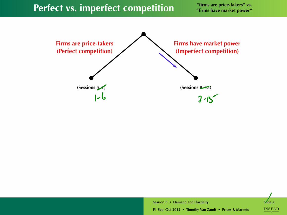
Perfect vs. imperfect competition “firms are price-takers” vs.“firms have market power”
(Sessions 5–7)
Firms are price-takers(Perfect competition)
(Sessions 8–15)
Firms have market power(Imperfect competition)
P1 Sep–Oct 2012 • Timothy Van Zandt • Prices & Markets
Session 7 • Demand and Elasticity Slide 2
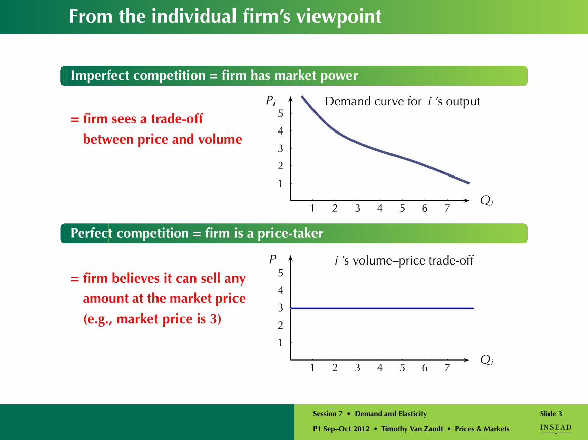
From the individual firm’s viewpoint
Imperfect competition = firm has market power
= firm sees a trade-offbetween price and volume
1
2
3
4
5
1 2 3 4 5 6 7Qi
Pi Demand curve for i ’s output
Perfect competition = firm is a price-taker
= firm believes it can sell anyamount at the market price(e.g., market price is 3)
1
2
3
4
5
1 2 3 4 5 6 7Qi
P i ’s volume–price trade-off
P1 Sep–Oct 2012 • Timothy Van Zandt • Prices & Markets
Session 7 • Demand and Elasticity Slide 3
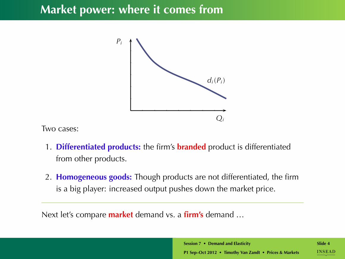
Market power: where it comes from
Qi
Pi
di (Pi )
Two cases:
1. Differentiated products: the firm’s branded product is differentiatedfrom other products.
2. Homogeneous goods: Though products are not differentiated, the firmis a big player: increased output pushes down the market price.
Next let’s compare market demand vs. a firm’s demand …
P1 Sep–Oct 2012 • Timothy Van Zandt • Prices & Markets
Session 7 • Demand and Elasticity Slide 4
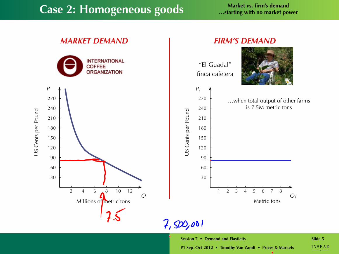
Case 2: Homogeneous goods Market vs. firm’s demand…starting with no market power
MARKET DEMAND
30
60
90
120
150
180
210
240
270
2 4 6 8 10 12
P
Q
US
Cen
tspe
rPo
und
Millions of metric tons
FIRM’S DEMAND
“El Guadal”finca cafetera
30
60
90
120
150
180
210
240
270
1 2 3 4 5 6 7 8
Pi
Qi
US
Cen
tspe
rPo
und
Metric tons
…when total output of other farmsis 7.5M metric tons
P1 Sep–Oct 2012 • Timothy Van Zandt • Prices & Markets
Session 7 • Demand and Elasticity Slide 5

Market power: Our simulation Market demand vs.firm’s demand
MARKET DEMAND
Q = 6000 − 100P
10
20
30
40
50
60
1 2 3 4 5 6
P
QThousands
FIRM’S DEMAND
When Q−i = 3173
10
20
30
40
50
60
20 40 60 80 100 120
Pi
Qi
P1 Sep–Oct 2012 • Timothy Van Zandt • Prices & Markets
Session 7 • Demand and Elasticity Slide 6
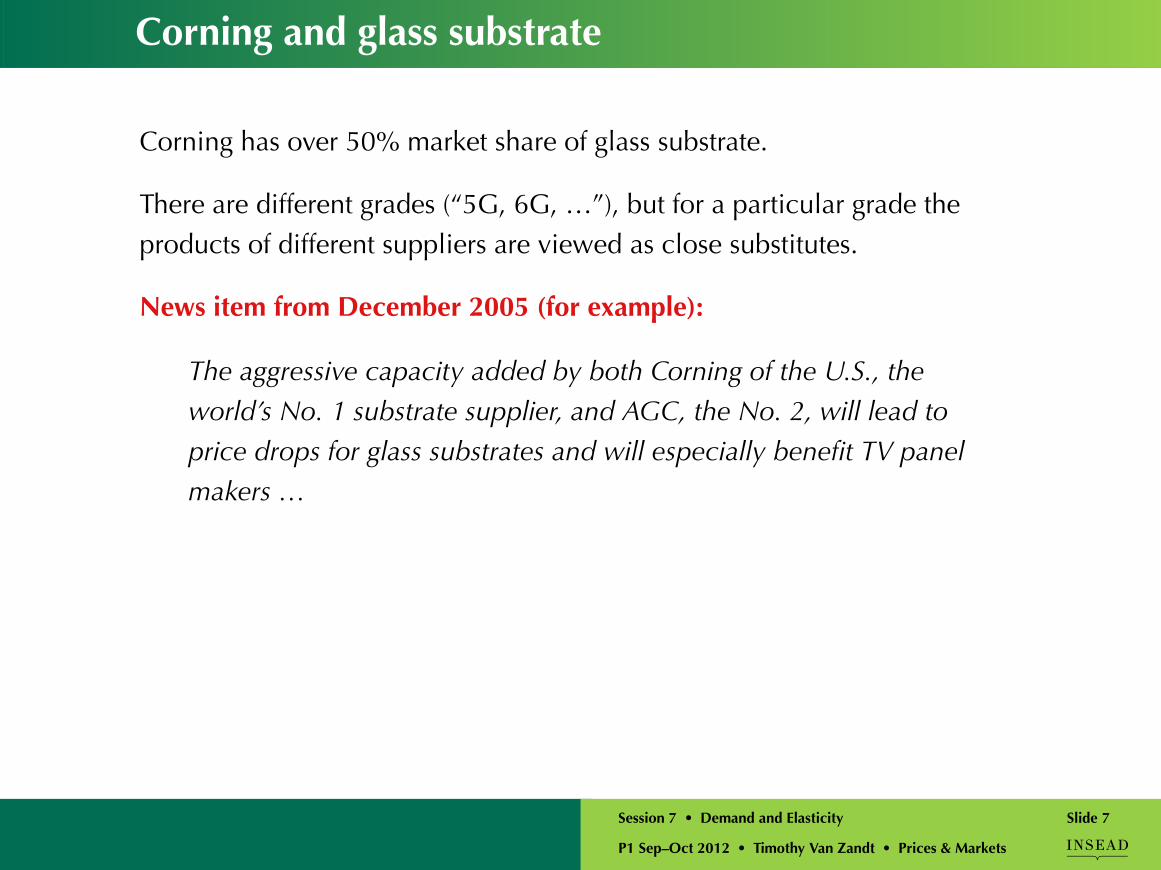
Corning and glass substrate
Corning has over 50% market share of glass substrate.
There are different grades (“5G, 6G, …”), but for a particular grade theproducts of different suppliers are viewed as close substitutes.
News item from December 2005 (for example):
The aggressive capacity added by both Corning of the U.S., theworld’s No. 1 substrate supplier, and AGC, the No. 2, will lead toprice drops for glass substrates and will especially benefit TV panelmakers …
P1 Sep–Oct 2012 • Timothy Van Zandt • Prices & Markets
Session 7 • Demand and Elasticity Slide 7
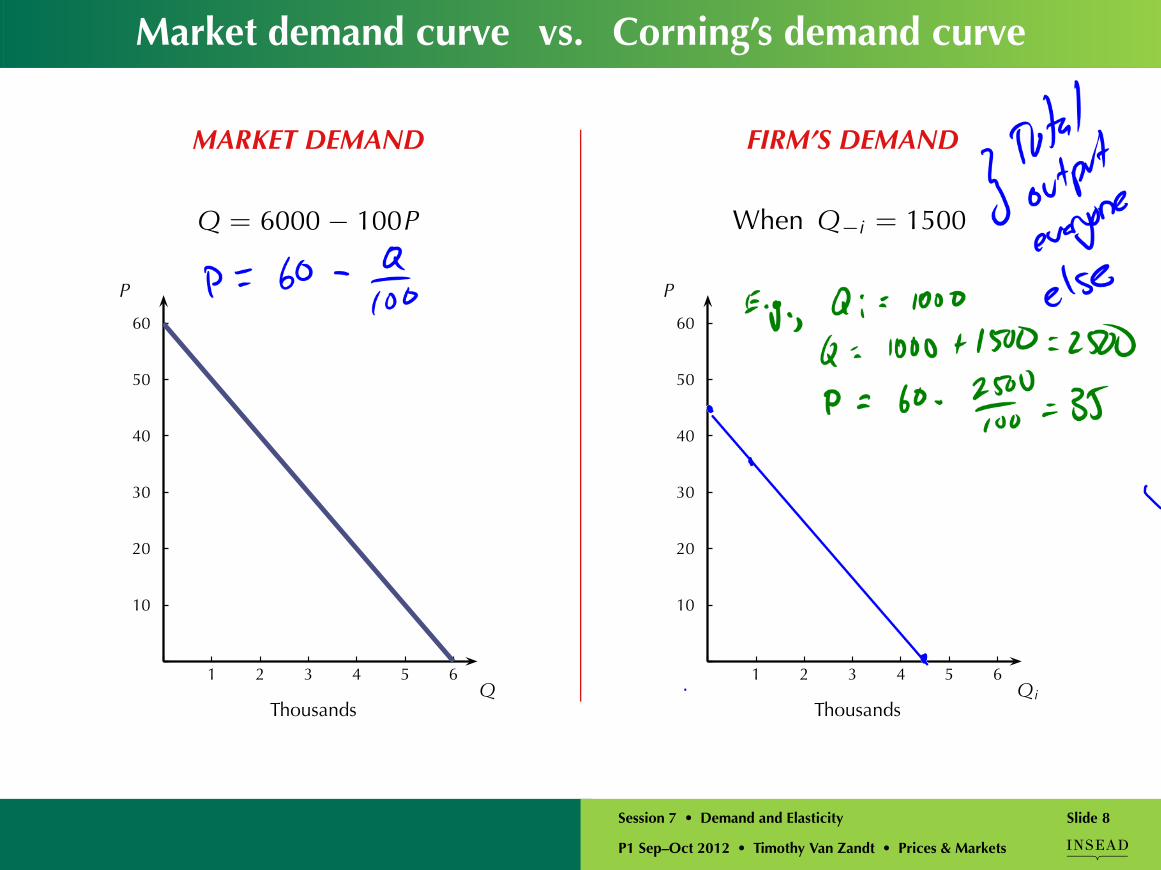
Market demand curve vs. Corning’s demand curve
MARKET DEMAND
Q = 6000 − 100P
10
20
30
40
50
60
1 2 3 4 5 6
P
QThousands
FIRM’S DEMAND
When Q−i = 1500
10
20
30
40
50
60
1 2 3 4 5 6
P
QiThousands
P1 Sep–Oct 2012 • Timothy Van Zandt • Prices & Markets
Session 7 • Demand and Elasticity Slide 8
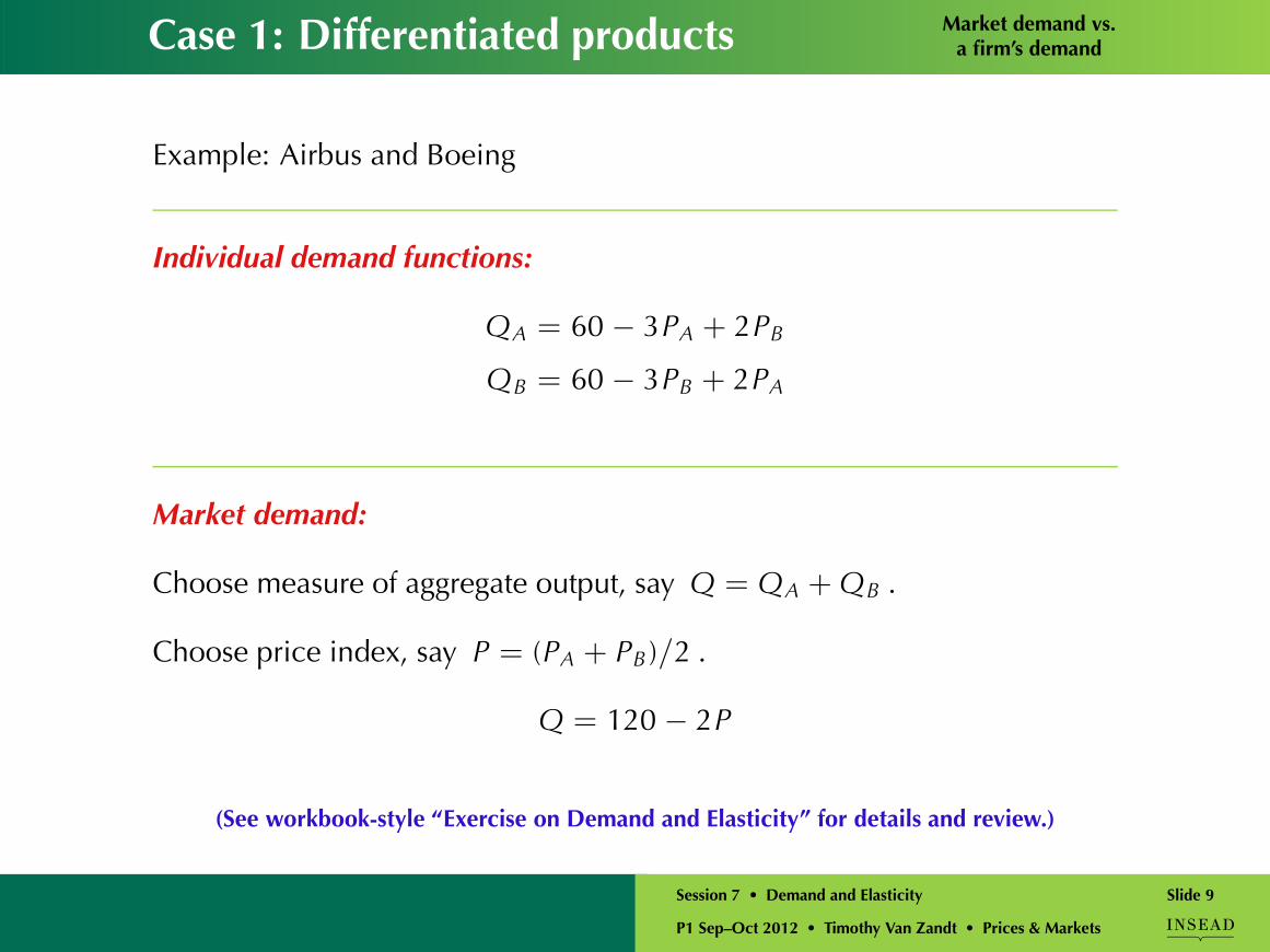
Case 1: Differentiated products Market demand vs.a firm’s demand
Example: Airbus and Boeing
Individual demand functions:
QA = 60 − 3PA + 2PB
QB = 60 − 3PB + 2PA
Market demand:
Choose measure of aggregate output, say Q = QA + QB .
Choose price index, say P = (PA + PB )/2 .
Q = 120 − 2P
(See workbook-style “Exercise on Demand and Elasticity” for details and review.)
P1 Sep–Oct 2012 • Timothy Van Zandt • Prices & Markets
Session 7 • Demand and Elasticity Slide 9

Topic 7: Demand and Elasticity
1✓ Market vs. firm’s demand
2➥ Elasticity and revenue
3 Numerical examples: Elasticity for linear and log-linear demand
4 Determinants of elasticity
5 Demand estimation exercise.
P1 Sep–Oct 2012 • Timothy Van Zandt • Prices & Markets
Session 7 • Demand and Elasticity Slide 10
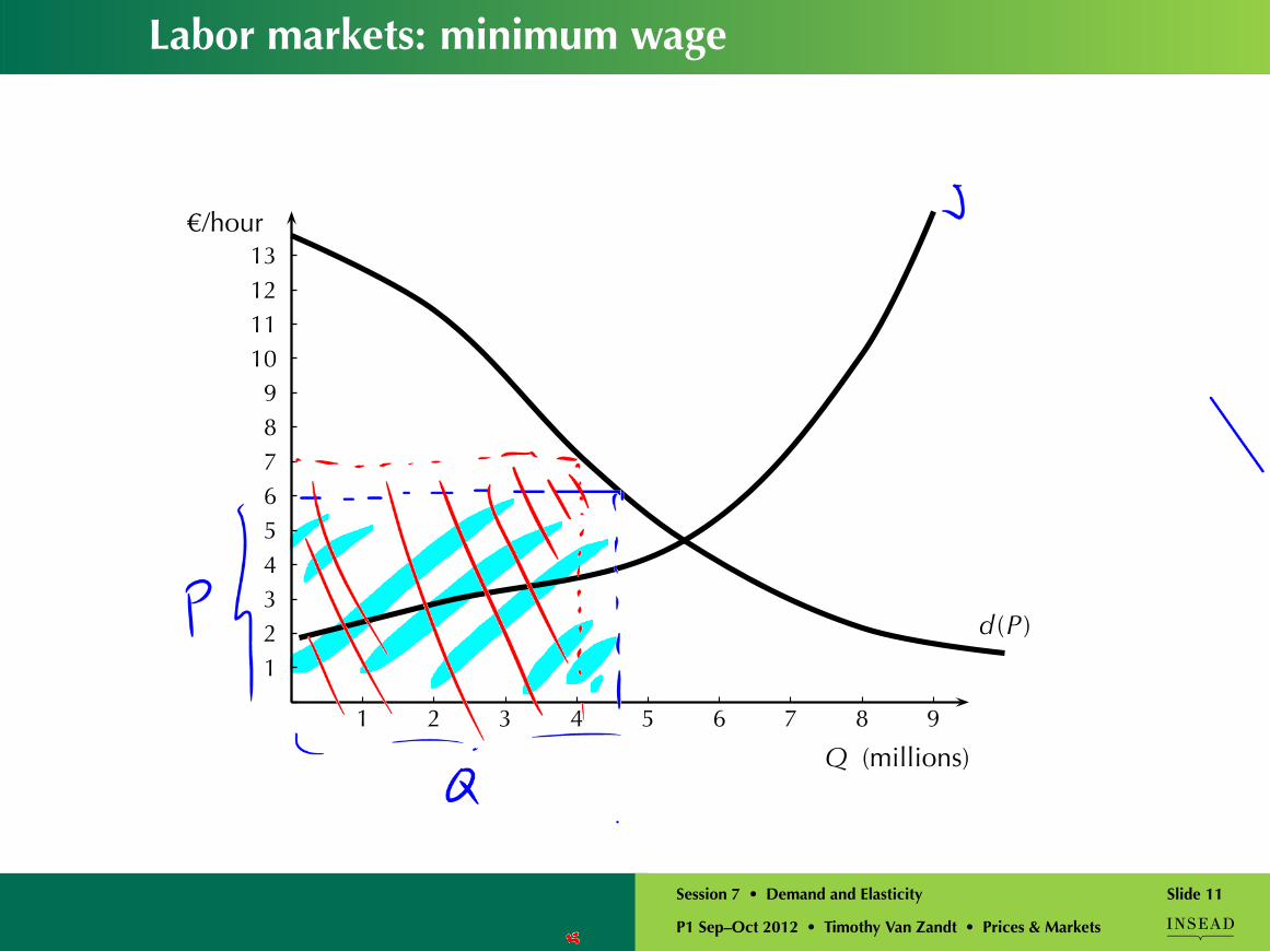
Labor markets: minimum wage
d (P )
123456789
10111213
1 2 3 4 5 6 7 8 9
Q (millions)
€/hour
P1 Sep–Oct 2012 • Timothy Van Zandt • Prices & Markets
Session 7 • Demand and Elasticity Slide 11

Key point: % changes matter
An increase in minimum wage has two effects on total wage bill:
P ↑ : Each worker is more expensive : wage bill ↑ by %ΔP
Q ↓ : Firms employ fewer workers : wage bill ↓ by %ΔQ
P1 Sep–Oct 2012 • Timothy Van Zandt • Prices & Markets
Session 7 • Demand and Elasticity Slide 12

Key point: % changes matter
An increase in minimum wage has two effects on total wage bill:
P ↑ : Each worker is more expensive : wage bill ↑ by %ΔP
Q ↓ : Firms employ fewer workers : wage bill ↓ by %ΔQ
Net effect depends on which is greater:
%ΔP or %ΔQ
P1 Sep–Oct 2012 • Timothy Van Zandt • Prices & Markets
Session 7 • Demand and Elasticity Slide 12

Example: linear demand
123456789
1011121314151617
1 2 3 4 5 6 7 8
Q (millions)
€/hour
P1 Sep–Oct 2012 • Timothy Van Zandt • Prices & Markets
Session 7 • Demand and Elasticity Slide 13
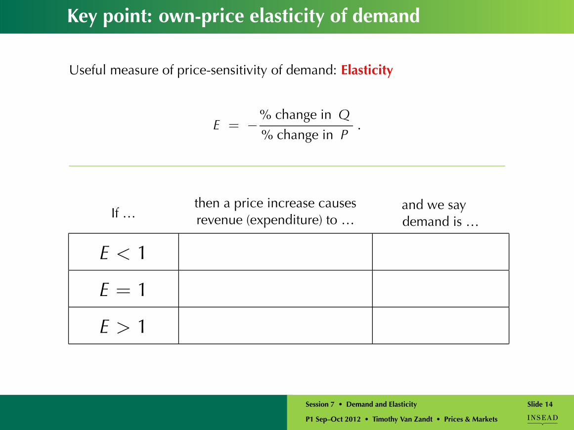
Key point: own-price elasticity of demand
Useful measure of price-sensitivity of demand: Elasticity
E = −% change in Q
% change in P.
If …then a price increase causesrevenue (expenditure) to …
and we saydemand is …
E < 1
E = 1
E > 1
P1 Sep–Oct 2012 • Timothy Van Zandt • Prices & Markets
Session 7 • Demand and Elasticity Slide 14
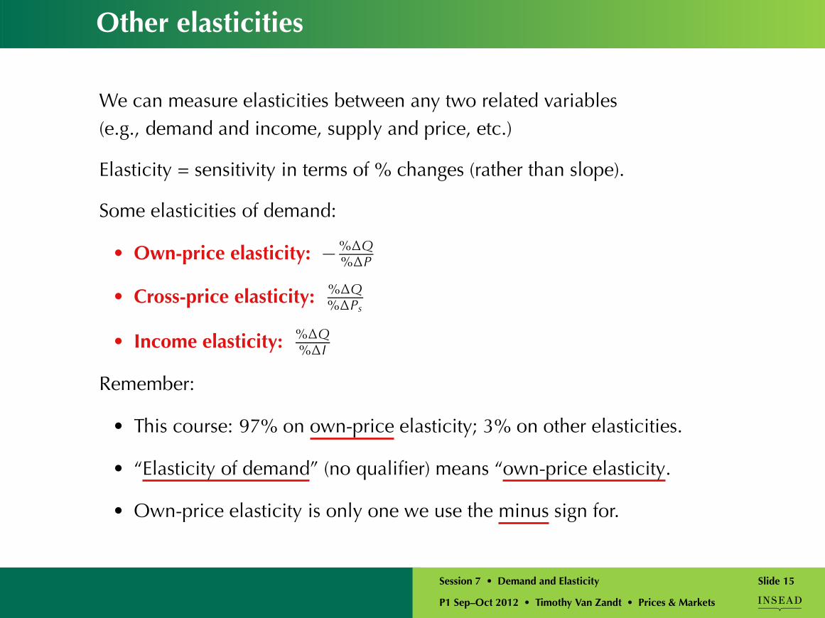
Other elasticities
We can measure elasticities between any two related variables(e.g., demand and income, supply and price, etc.)
Elasticity = sensitivity in terms of % changes (rather than slope).
Some elasticities of demand:
• Own-price elasticity: −%ΔQ%ΔP
• Cross-price elasticity: %ΔQ%ΔPs
• Income elasticity: %ΔQ%ΔI
Remember:
• This course: 97% on own-price elasticity; 3% on other elasticities.
• “Elasticity of demand” (no qualifier) means “own-price elasticity.
• Own-price elasticity is only one we use the minus sign for.
P1 Sep–Oct 2012 • Timothy Van Zandt • Prices & Markets
Session 7 • Demand and Elasticity Slide 15
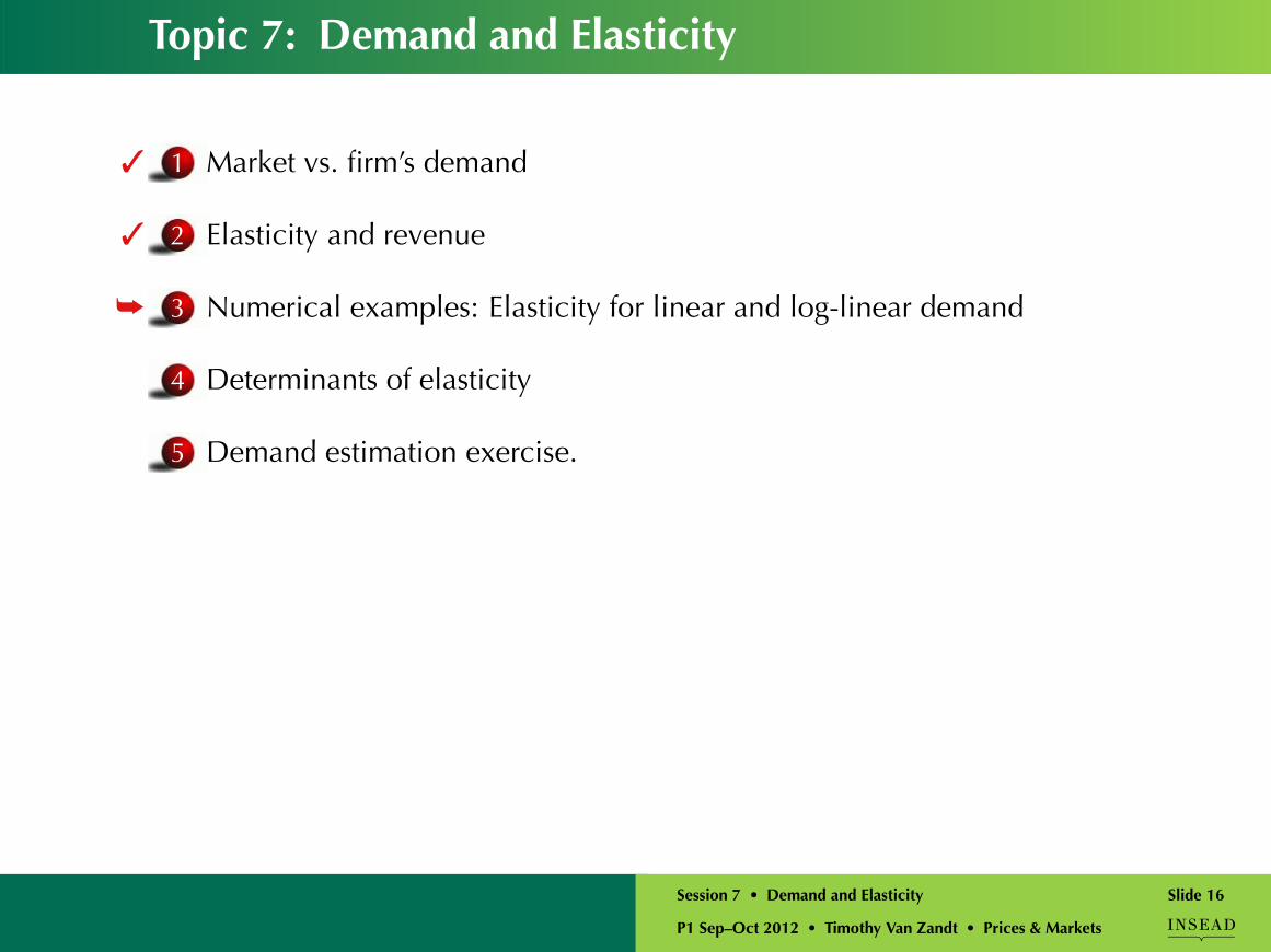
Topic 7: Demand and Elasticity
1✓ Market vs. firm’s demand
2✓ Elasticity and revenue
3➥ Numerical examples: Elasticity for linear and log-linear demand
4 Determinants of elasticity
5 Demand estimation exercise.
P1 Sep–Oct 2012 • Timothy Van Zandt • Prices & Markets
Session 7 • Demand and Elasticity Slide 16
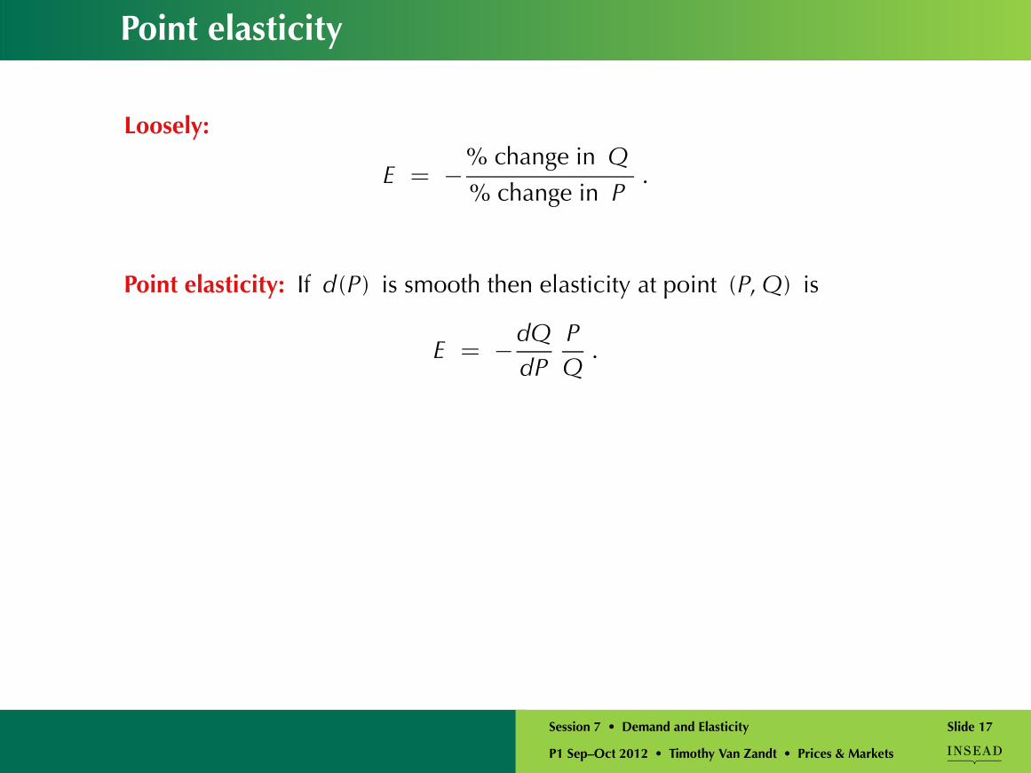
Point elasticity
Loosely:
E = −% change in Q
% change in P.
Point elasticity: If d (P ) is smooth then elasticity at point (P, Q) is
E = −dQdP
PQ
.
P1 Sep–Oct 2012 • Timothy Van Zandt • Prices & Markets
Session 7 • Demand and Elasticity Slide 17
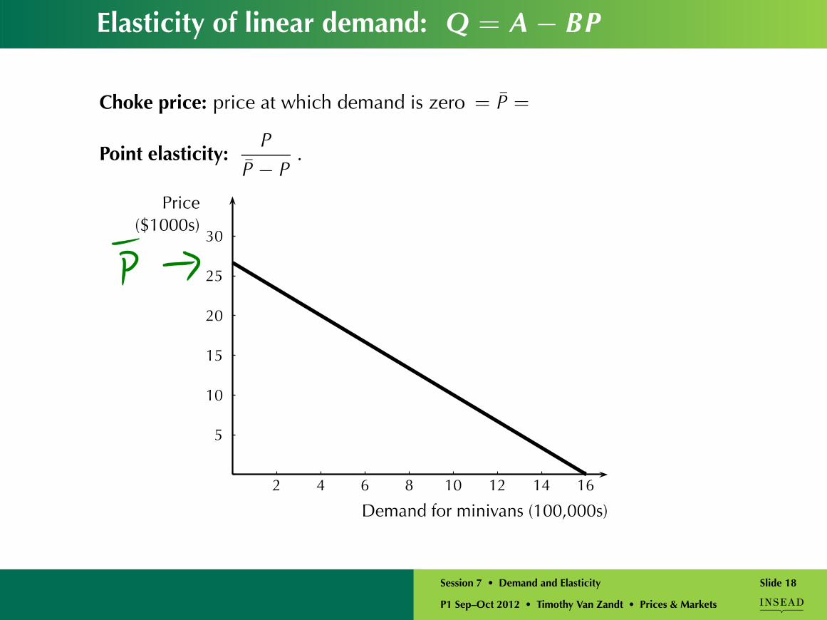
Elasticity of linear demand: Q = A − BP
Choke price: price at which demand is zero = P̄ =
Point elasticity:P
P̄ − P.
5
10
15
20
25
30
2 4 6 8 10 12 14 16
Price($1000s)
Demand for minivans (100,000s)
P1 Sep–Oct 2012 • Timothy Van Zandt • Prices & Markets
Session 7 • Demand and Elasticity Slide 18
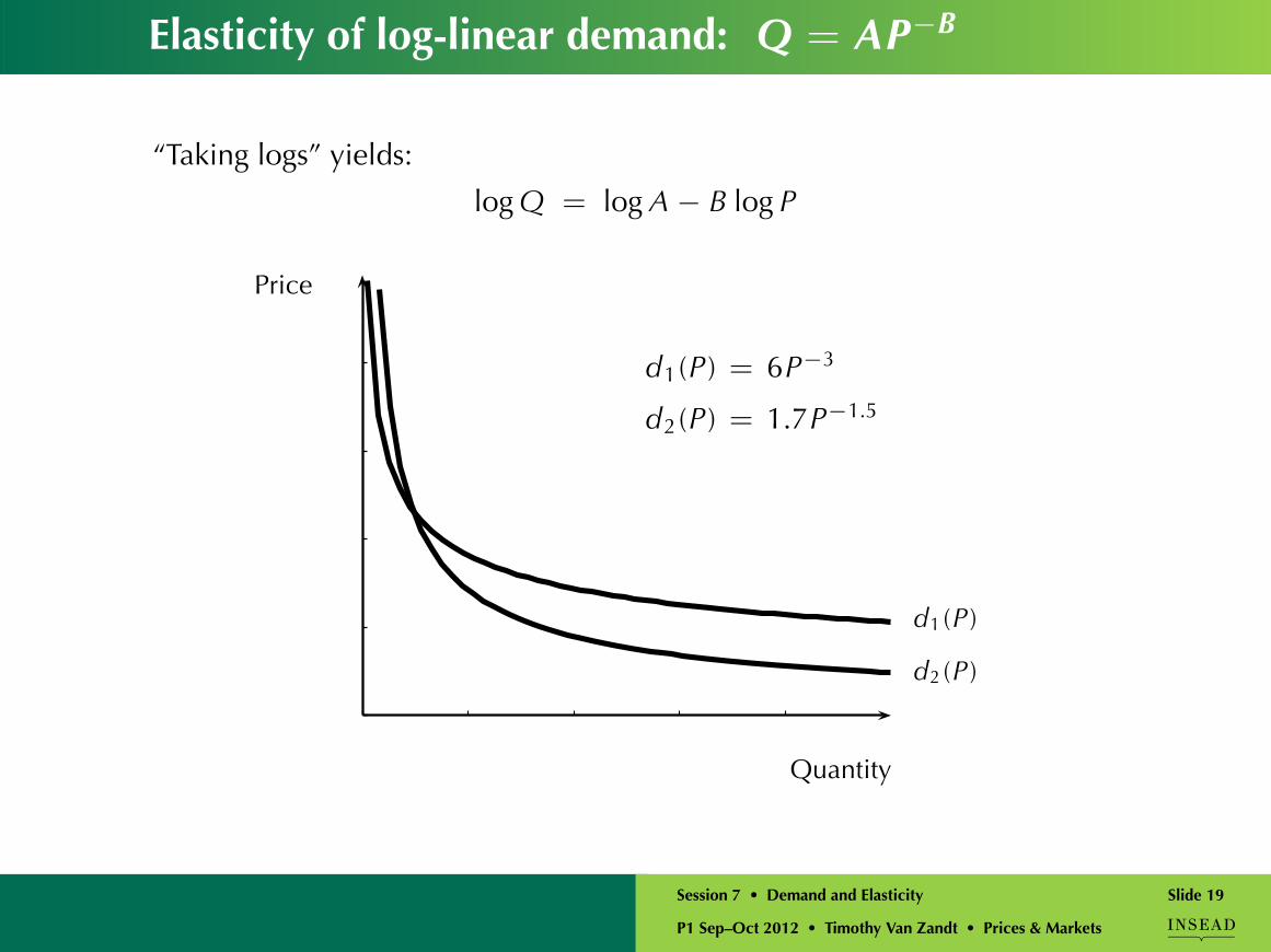
Elasticity of log-linear demand: Q = AP−B
“Taking logs” yields:
log Q = log A − B log P
Price
Quantity
d1 (P )
d2 (P )
d1(P ) = 6P−3
d2(P ) = 1.7P−1.5
P1 Sep–Oct 2012 • Timothy Van Zandt • Prices & Markets
Session 7 • Demand and Elasticity Slide 19

Topic 7: Demand and Elasticity
1✓ Market vs. firm’s demand
2✓ Elasticity and revenue
3✓ Numerical examples: Elasticity for linear and log-linear demand
4➥ Determinants of elasticity
5 Demand estimation exercise.
P1 Sep–Oct 2012 • Timothy Van Zandt • Prices & Markets
Session 7 • Demand and Elasticity Slide 20
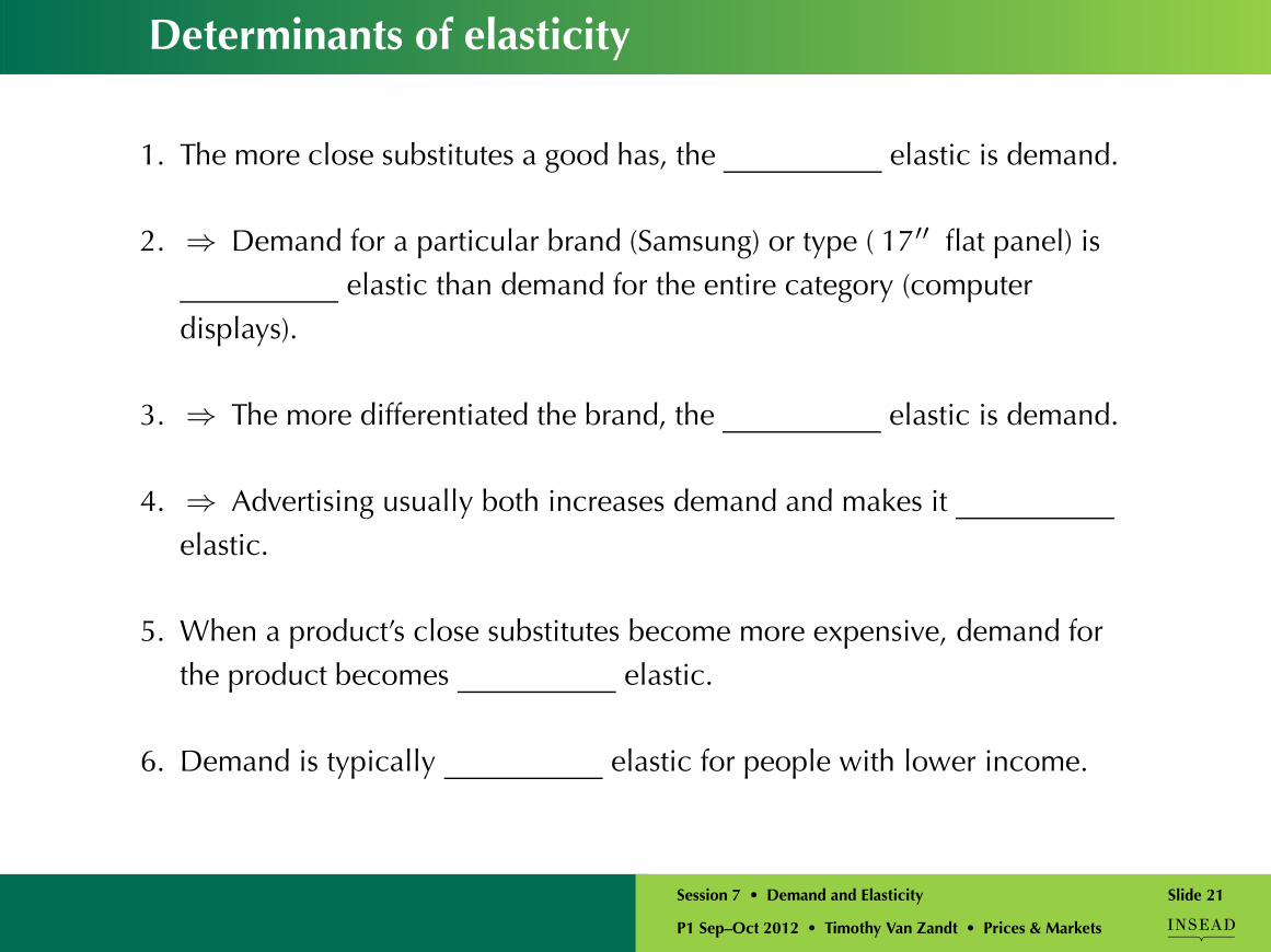
Determinants of elasticity
1. The more close substitutes a good has, the elastic is demand.
2. ⇒ Demand for a particular brand (Samsung) or type ( 17′′ flat panel) iselastic than demand for the entire category (computer
displays).
3. ⇒ The more differentiated the brand, the elastic is demand.
4. ⇒ Advertising usually both increases demand and makes itelastic.
5. When a product’s close substitutes become more expensive, demand forthe product becomes elastic.
6. Demand is typically elastic for people with lower income.
P1 Sep–Oct 2012 • Timothy Van Zandt • Prices & Markets
Session 7 • Demand and Elasticity Slide 21
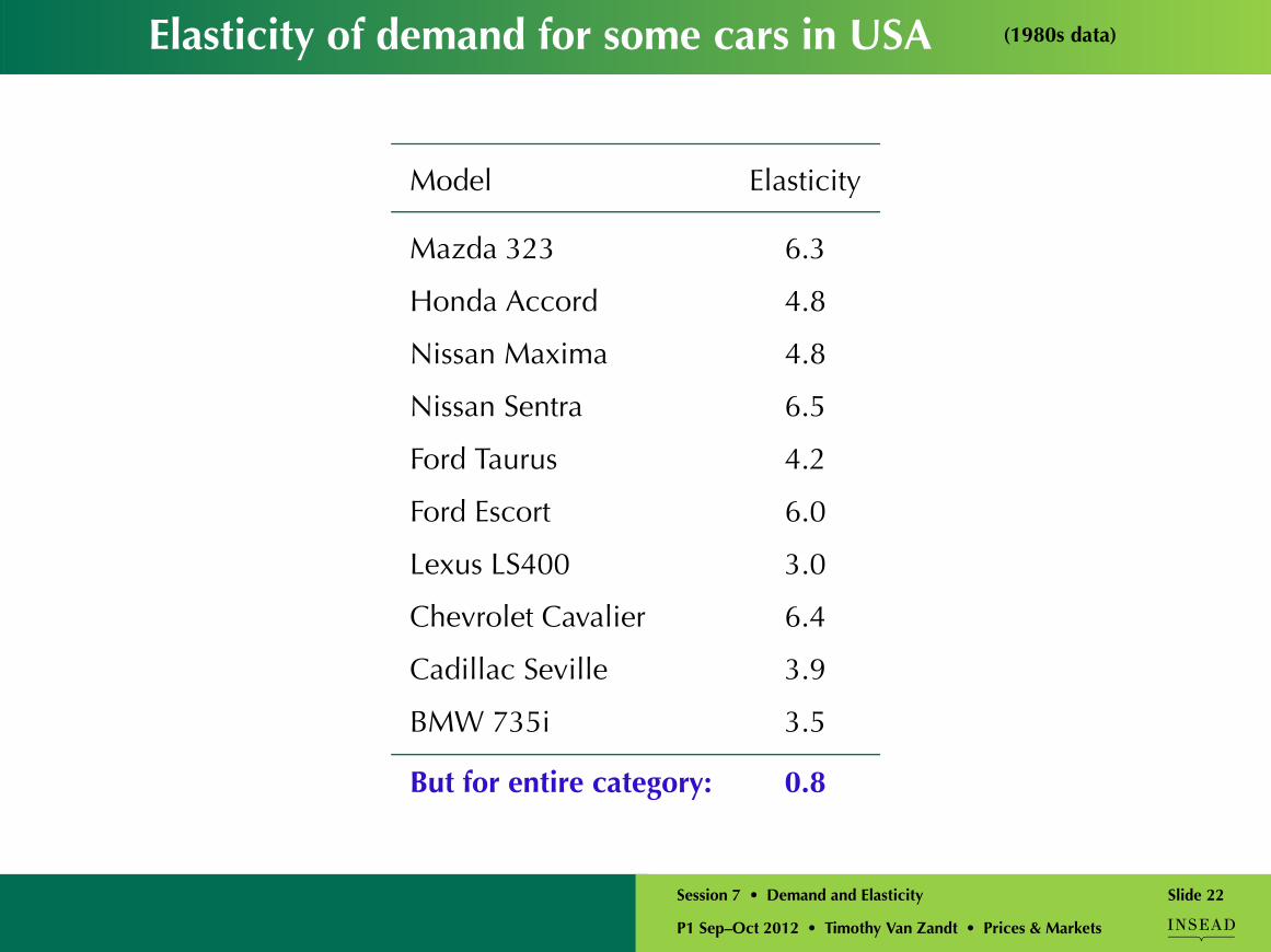
Elasticity of demand for some cars in USA (1980s data)
Model Elasticity
Mazda 323 6.3
Honda Accord 4.8
Nissan Maxima 4.8
Nissan Sentra 6.5
Ford Taurus 4.2
Ford Escort 6.0
Lexus LS400 3.0
Chevrolet Cavalier 6.4
Cadillac Seville 3.9
BMW 735i 3.5
But for entire category: 0.8
P1 Sep–Oct 2012 • Timothy Van Zandt • Prices & Markets
Session 7 • Demand and Elasticity Slide 22

Topic 7: Demand and Elasticity
1✓ Market vs. firm’s demand
2✓ Elasticity and revenue
3✓ Numerical examples: Elasticity for linear and log-linear demand
4✓ Determinants of elasticity
5➥ Demand estimation exercise.
P1 Sep–Oct 2012 • Timothy Van Zandt • Prices & Markets
Session 7 • Demand and Elasticity Slide 23
Estimating demand: Get some data
1. Consumer surveys.
2. Consumer focus groups.
3. Market experiments.
4. Historical (real) data: cross-section, time-series, or both (panel).
P1 Sep–Oct 2012 • Timothy Van Zandt • Prices & Markets
Session 7 • Demand and Elasticity Slide 24
Estimating demand: Fit a curve
1. Write down model (equation) for demand, with unspecifiedcoefficients.
2. Fit line or curve to data points using statistical techniques (regression).
It’s all approximate:
• Include most relevant variables.
• Pick a simple functional form without too many coefficients.
P1 Sep–Oct 2012 • Timothy Van Zandt • Prices & Markets
Session 7 • Demand and Elasticity Slide 25

Two common parametric forms
Linear
Q = A − B1P + B2Ps + B3 I + · · ·e.g.
FPR = −0.02 − 0.8PF + 0.4PM − 0.07MPR + 0.35GDP
Log-linear (constant elasticity)
Q = A P−B1 PB2s IB3 · · ·
taking logs yields
log Q = log A − B1 log P + B2 log Ps + B3 log I + · · ·
P1 Sep–Oct 2012 • Timothy Van Zandt • Prices & Markets
Session 7 • Demand and Elasticity Slide 26

Demand for US Gasoline Consumption
Variables:
GPC = Per-capita U.S. gasoline consumption
PG = Price index for gasoline
Y = Per capita disposable income
PNC = Price index for new cars
PUC = Price index for used cars
Model:
GPC = A PGB1 YB2 PNCB3 PUCB4
Or:
log GPC = log A + B1 log PG + B2 log Y + B3 log PNC + B4 log PUC
P1 Sep–Oct 2012 • Timothy Van Zandt • Prices & Markets
Session 7 • Demand and Elasticity Slide 27
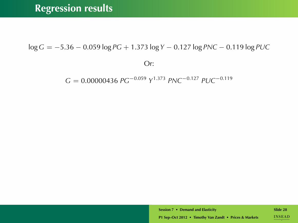
Regression results
log G = −5.36 − 0.059 log PG + 1.373 log Y − 0.127 log PNC − 0.119 log PUC
Or:
G = 0.00000436 PG−0.059 Y1.373 PNC−0.127 PUC−0.119
P1 Sep–Oct 2012 • Timothy Van Zandt • Prices & Markets
Session 7 • Demand and Elasticity Slide 28
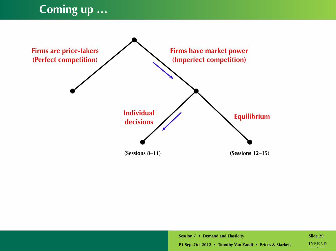
Coming up …
Firms are price-takers(Perfect competition)
Firms have market power(Imperfect competition)
(Sessions 8–11)
Individualdecisions
(Sessions 12–15)
Equilibrium
P1 Sep–Oct 2012 • Timothy Van Zandt • Prices & Markets
Session 7 • Demand and Elasticity Slide 29
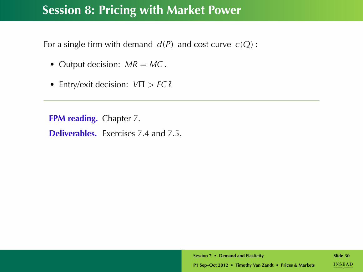
Session 8: Pricing with Market Power
For a single firm with demand d (P ) and cost curve c (Q) :
• Output decision: MR = MC .
• Entry/exit decision: VΠ > FC ?
FPM reading. Chapter 7.
Deliverables. Exercises 7.4 and 7.5.
P1 Sep–Oct 2012 • Timothy Van Zandt • Prices & Markets
Session 7 • Demand and Elasticity Slide 30