yoshiharu ishikawa (nagoya university) yoji machida (university of tsukuba) hiroyuki kitagawa...

Yoshiharu Ishikawa (Nagoya University)

Yoji Machida (University of Tsukuba)

Hiroyuki Kitagawa (University of Tsukuba)

A Dynamic Mobility Histogram Construction Method

Based on Markov Chains

2

Outline

• Background and Objectives• Modeling Movement Patterns• Mobility Histogram: Logical Structure• Mobility Histogram: Physical Structure• Experimental Results• Conclusions

3

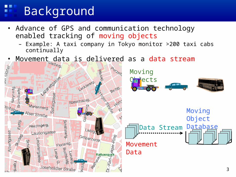
Background• Advance of GPS and communication technology enabled

tracking of moving objects– Example: A taxi company in Tokyo monitor >200 taxi cabs continually

• Movement data is delivered as a data stream

Data Stream

Movement Data

Moving ObjectDatabase

Moving Objects

4

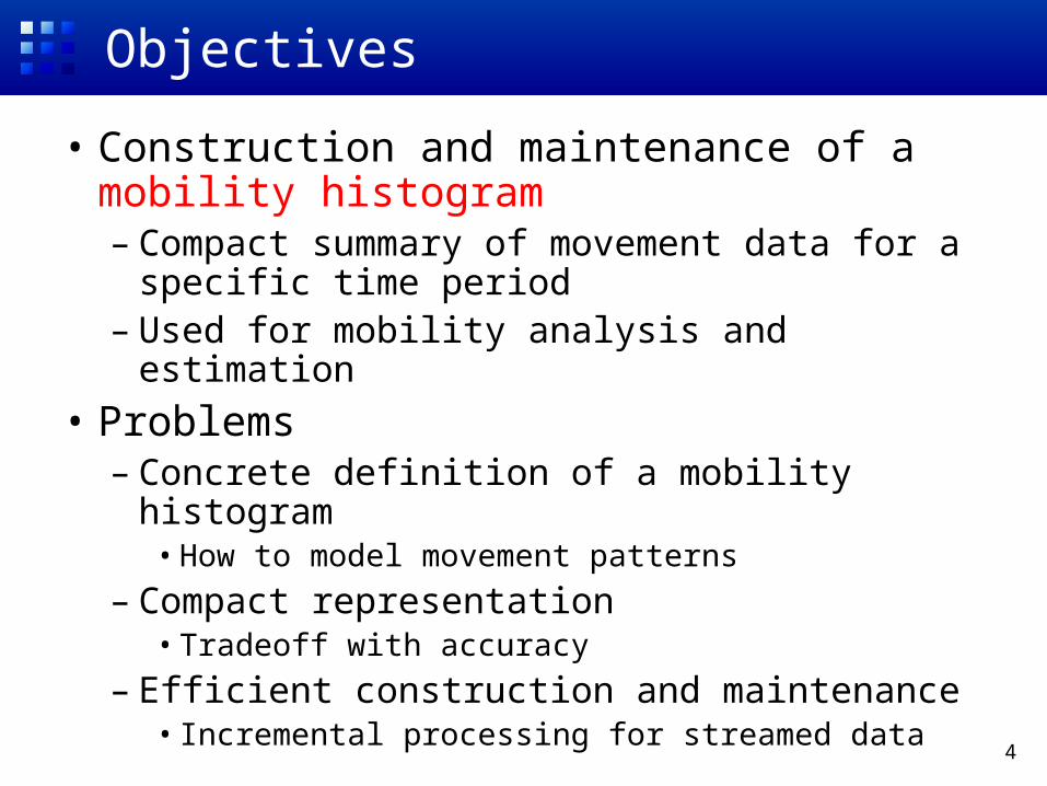
Objectives

• Construction and maintenance of a mobility histogram– Compact summary of movement data for a

specific time period– Used for mobility analysis and estimation

• Problems– Concrete definition of a mobility histogram

• How to model movement patterns

– Compact representation• Tradeoff with accuracy

– Efficient construction and maintenance• Incremental processing for streamed data

5

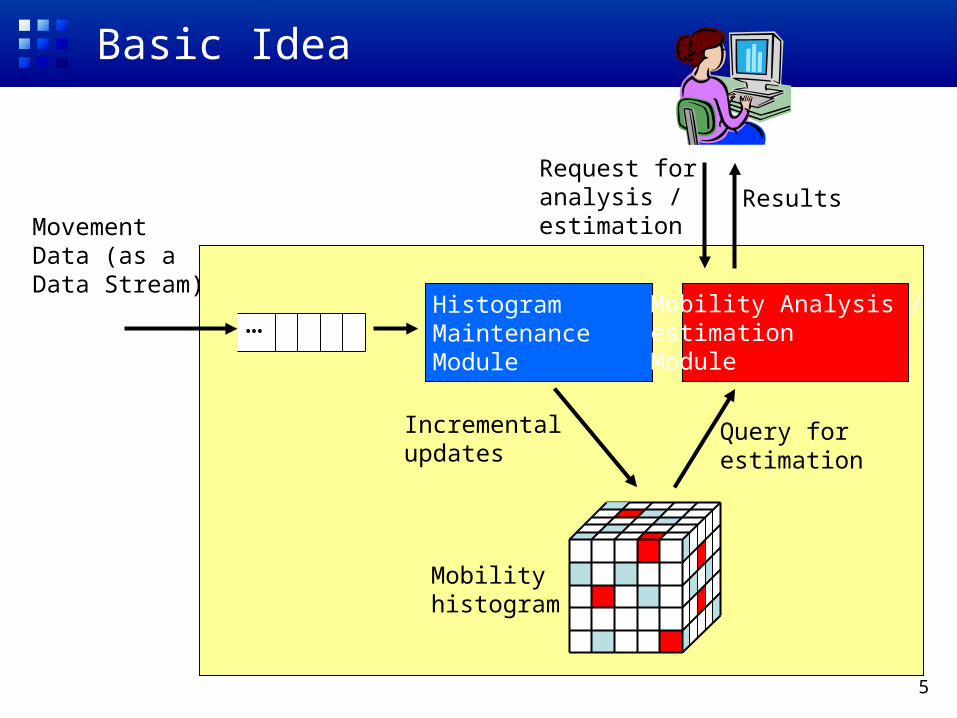
MovementData (as aData Stream)

Mobilityhistogram

Histogram MaintenanceModule

Incrementalupdates

Mobility Analysis /estimationModule

Query forestimation

…

Request foranalysis /estimation

Results

Basic Idea

6

Outline


7

Approach

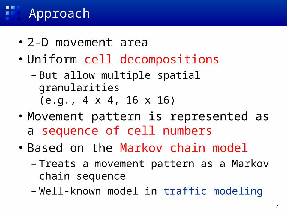
• 2-D movement area

• Uniform cell decompositions– But allow multiple spatial granularities

(e.g., 4 x 4, 16 x 16)

• Movement pattern is represented as a sequence of cell numbers

• Based on the Markov chain model– Treats a movement pattern as a Markov chain

sequence– Well-known model in traffic modeling

8

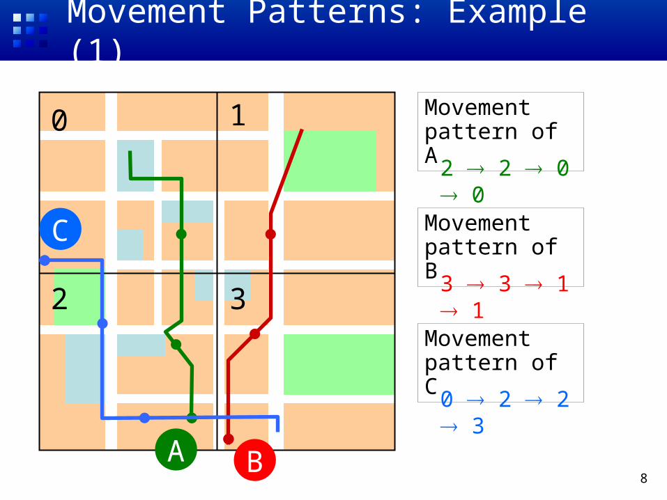
Movement Patterns: Example (1)

Movement pattern of A

Movement pattern of B

Movement pattern of C

2 2 0 0

3 3 1 1

0 2 2 3

0 1

2 3

A B

C

9

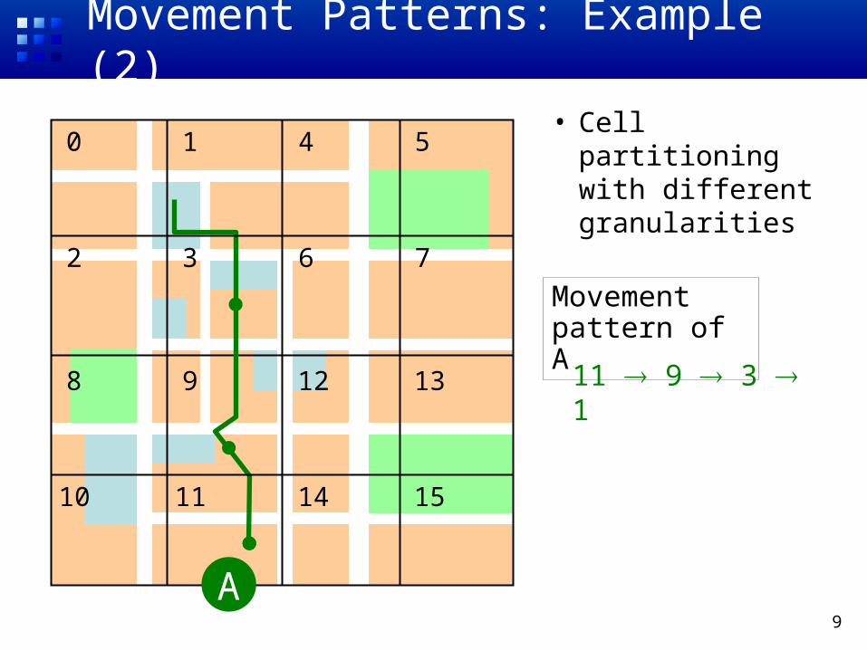
Movement Patterns: Example (2)

• Cell partitioning with different granularities

Movement pattern of A

11 9 3 1

A

0

2

8

10

1

3

9

11

4

6

12

14

5

7

13

15

10

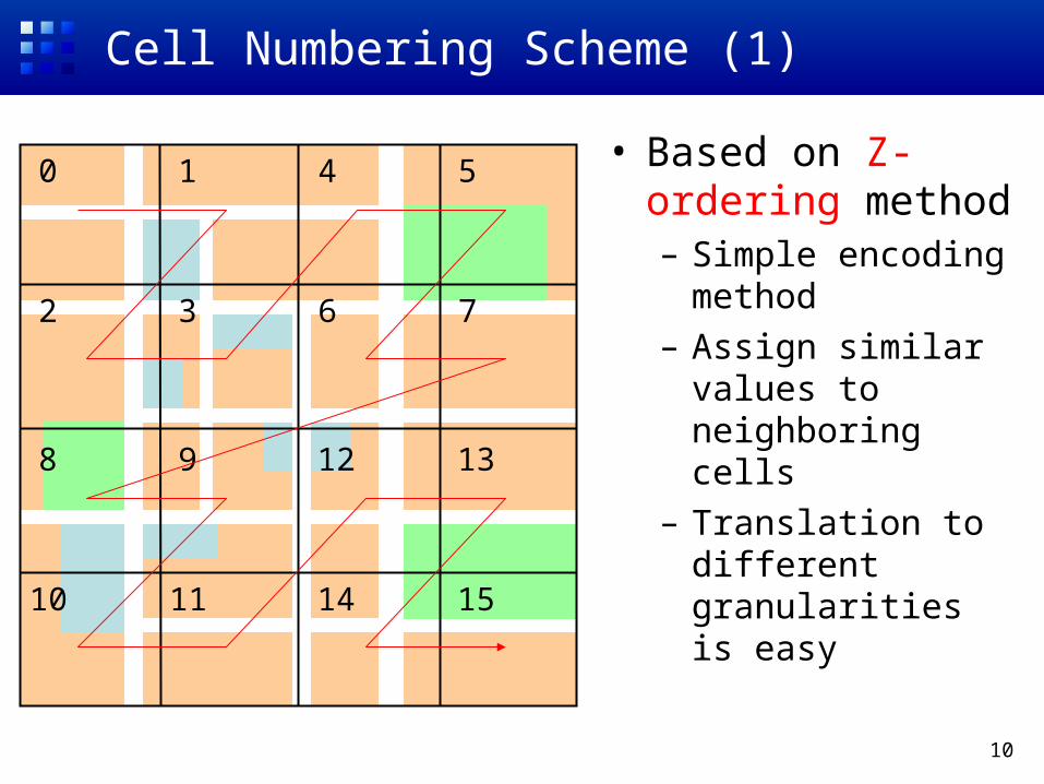
Cell Numbering Scheme (1)

• Based on Z-ordering method– Simple encoding

method– Assign similar values

to neighboring cells– Translation to

different granularities is easy

0

2

8

10

1

3

9

11

4

6

12

14

5

7

13

15

11

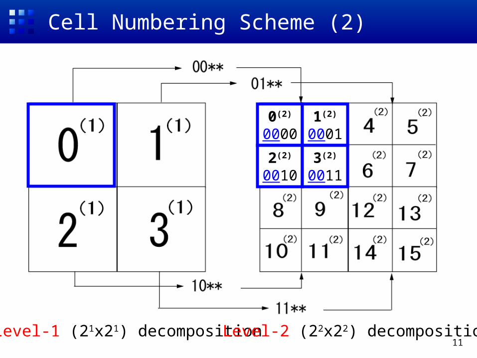
Cell Numbering Scheme (2)

0(2)

00001(2)

0001

2(2)

00103(2)

0011

Level-1 (21x21) decomposition Level-2 (22x22) decomposition

12

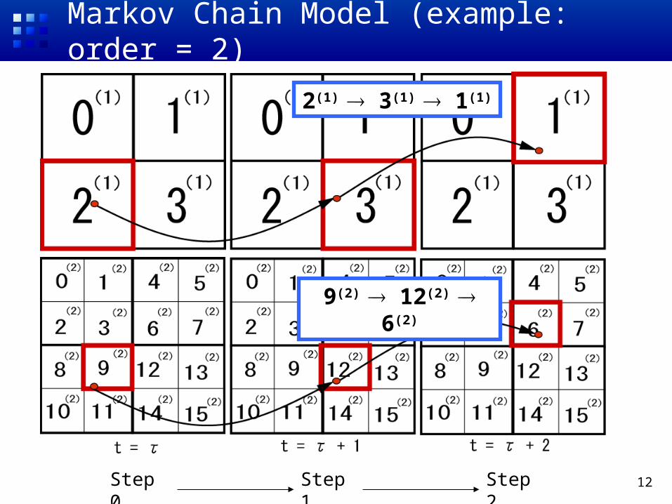
Markov Chain Model (example: order = 2)

Step 0 Step 1 Step 2

2(1) 3(1) 1(1)

9(2) 12(2) 6(2)

13

Outline


14

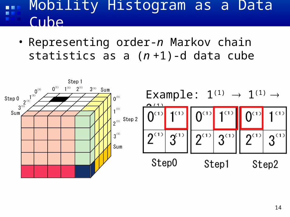
Mobility Histogram as a Data Cube

• Representing order-n Markov chain statistics as a (n +1)-d data cube

Example: 1(1) 1(1) 0(1)

15

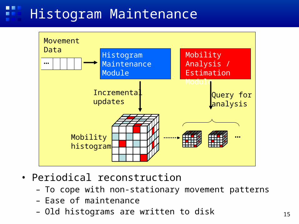
MovementData

Mobilityhistogram

Histogram MaintenanceModule

Incrementalupdates

Mobility Analysis /EstimationModule

Query foranalysis

…

Histogram Maintenance

…

• Periodical reconstruction– To cope with non-stationary movement patterns– Ease of maintenance– Old histograms are written to disk

16

Outline


17

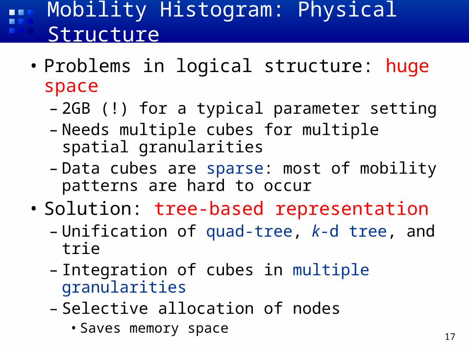
Mobility Histogram: Physical Structure

• Problems in logical structure: huge space– 2GB (!) for a typical parameter setting– Needs multiple cubes for multiple spatial

granularities– Data cubes are sparse: most of mobility

patterns are hard to occur

• Solution: tree-based representation– Unification of quad-tree, k-d tree, and trie– Integration of cubes in multiple granularities– Selective allocation of nodes

• Saves memory space

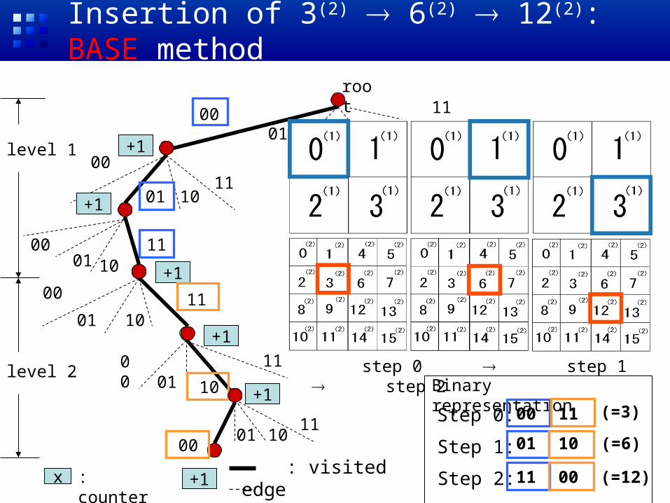
10

root

x : counter

0001

11

01

11

10

01

level 1

level 2Binary representation

Step 0:

Step 1:

Step 2:

00 11

01 10

11 00

(=3)

(=6)

(=12) : visited edge : non-visited edge

00

1011

0001

11

00

01 10

0100 11

0011

+1

+1

+1

+1

+1

+1

step 0 step 1 step 2

10

Insertion of 3(2) 6(2) 12(2): BASE method

19

Approximated Histogram (APR)

• Problem of the BASE method– Memory size requirement is still high

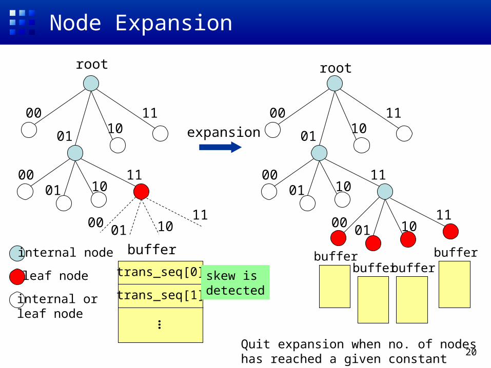
• Approximated method (APR)– Compact histogram construction by adaptive

tree expansion• Allocate a buffer for each leaf node• If skew is observed, the leaf node is expanded2 statistics is used to check the non-uniformity

– Inherited the idea from decision tree construction from streamed data (e.g., VFDT)

20

Node Expansion

00

0001

0110

11

1011

trans_seq[0]

trans_seq[1]

…

buffer

00

0001

0110

11

1011

0001 10

11

bufferbuffer buffer

buffer

expansion

skew isdetected

root root

internal node

leaf node

internal orleaf node

0001 10

11

Quit expansion when no. of nodeshas reached a given constant

21

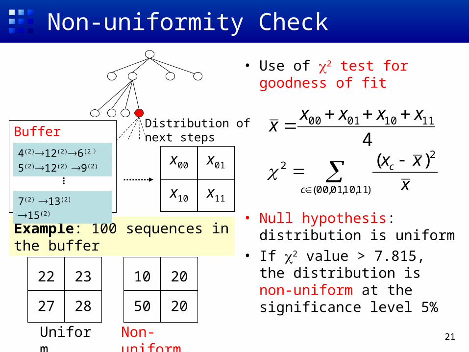
Example: 100 sequences in the buffer

Non-uniformity Check

• Use of 2 test for goodness of fit

• Null hypothesis: distribution is uniform

• If 2 value > 7.815, the distribution is non-uniform at the significance level 5%

411100100 xxxx

x

Buffer

…5(2)12(2) 9(2)

7(2) 13(2) 15(2)

4(2)12(2)6(2 ）

)11,10,01,00(

22 )(

c

c

x

xx

22 23

27 28

10 20

50 20

Uniform Non-uniform

x00 x01

x10 x11

Distribution ofnext steps

22

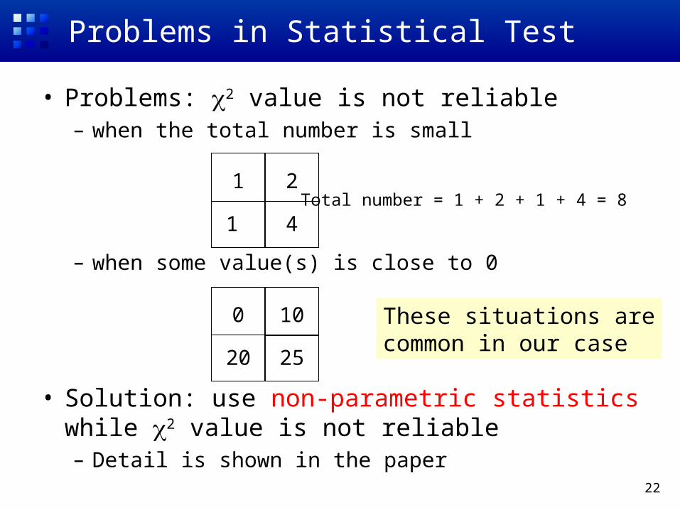
Problems in Statistical Test

• Problems: 2 value is not reliable– when the total number is small

– when some value(s) is close to 0

• Solution: use non-parametric statistics while 2 value is not reliable– Detail is shown in the paper

1 2

1 4Total number = 1 + 2 + 1 + 4 = 8

0 10

20 25

These situations arecommon in our case

23

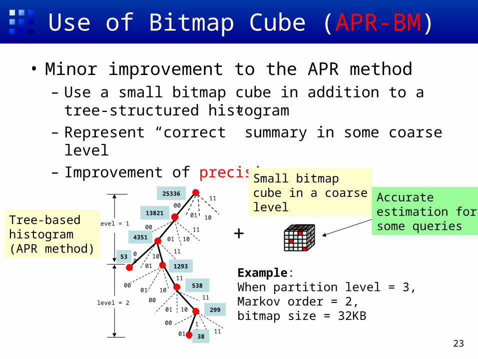
• Minor improvement to the APR method– Use a small bitmap cube in addition to a tree-

structured histogram– Represent “correct” summary in some coarse level– Improvement of precision

Use of Bitmap Cube (APR-BM)

level = 1

level = 2

10

00

01

01

10

11

10

01

00

10

11

00

01

11

0001 10

01

00 11

00

11

10

1125336

13821

4351

1293

538

299

53

38

Tree-basedhistogram(APR method)

+

Small bitmapcube in a coarselevel

Example: When partition level = 3,Markov order = 2,bitmap size = 32KB

Accurateestimation forsome queries

24

Outline


25

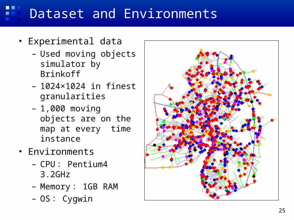
Dataset and Environments

• Experimental data– Used moving objects

simulator by Brinkoff

– 1024×1024 in finest granularities

– 1,000 moving objects are on the map at every time instance

• Environments– CPU： Pentium4

3.2GHz

– Memory： 1GB RAM

– OS： Cygwin

26

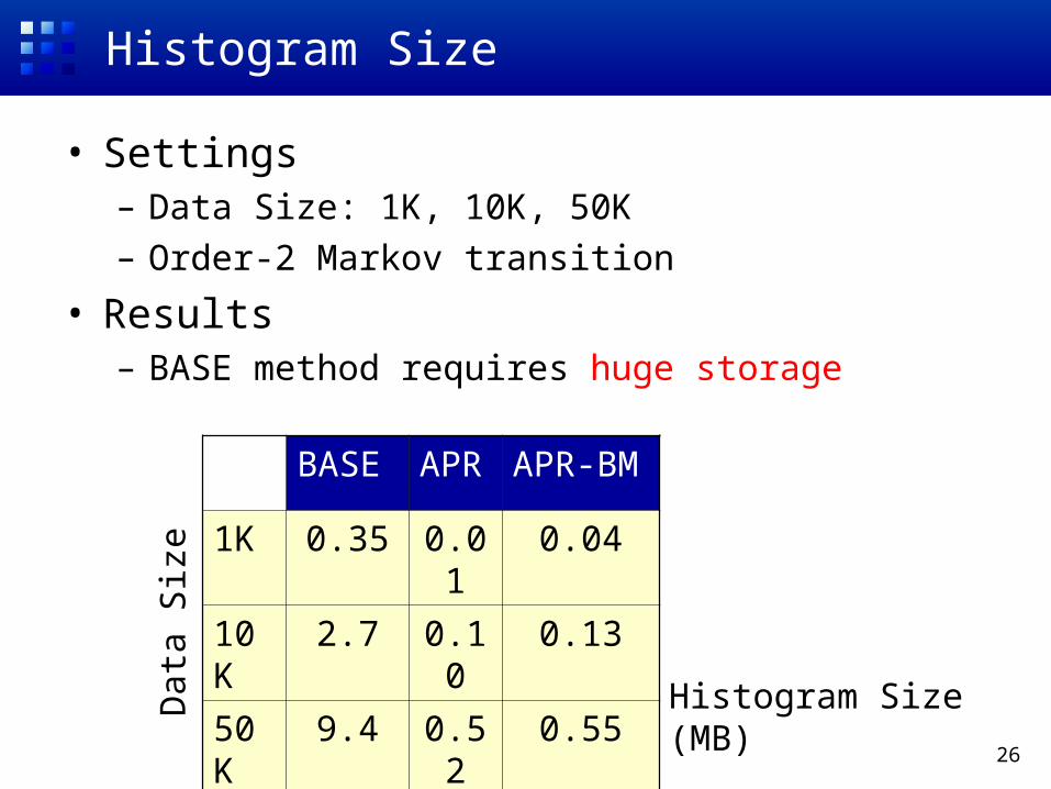
Histogram Size

• Settings– Data Size: 1K, 10K, 50K– Order-2 Markov transition

• Results– BASE method requires huge storage

BASE APR APR-BM

1K 0.35 0.01 0.04

10K 2.7 0.10 0.13

50K 9.4 0.52 0.55Dat

a S

ize

Histogram Size (MB)

27

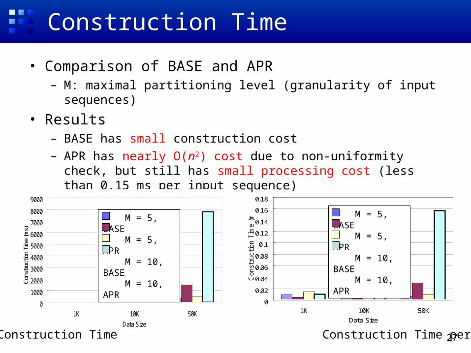
Construction Time

• Comparison of BASE and APR– M: maximal partitioning level (granularity of input sequences)

• Results– BASE has small construction cost– APR has nearly O(n2) cost due to non-uniformity check, but still

has small processing cost (less than 0.15 ms per input sequence)

0

0.02

0.04

0.06

0.08

0.1

0.12

0.14

0.16

0.18

1K 10K 50K

Data Size

Const

ruction T

ime (m

s)

5( )素朴な方式5( )近似方式10( )素朴な方式10( )近似方式

0

1000

2000

3000

4000

5000

6000

7000

8000

9000

1K 10K 50K

Data Size

Cons

truct

ion

Tim

e (m

s)

5( )素朴な方式5( )近似方式10( )素朴な方式10( )近似方式

M = 5, BASE M = 5, APR M = 10, BASE M = 10, APR

M = 5, BASE M = 5, APR M = 10, BASE M = 10, APR

Construction Time Construction Time per Sequence

28

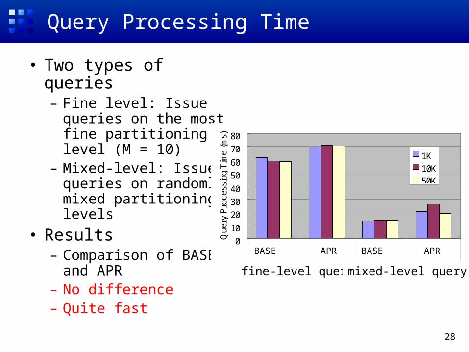
Query Processing Time

• Two types of queries– Fine level: Issue

queries on the most fine partitioning level (M = 10)

– Mixed-level: Issue queries on randomly mixed partitioning levels

• Results– Comparison of BASE

and APR– No difference– Quite fast

010

203040

5060

7080

素朴な方式近似方式素朴な方式近似方式

最大空間分割レベルと一致する問合せ

最大空間分割レベルよりも粗い問合せ

問合せパターン

Que

ry P

roce

ssin

g Ti

me

(ms)

1K10K50K

BASE BASE APR APR

fine-level query

mixed-level query

29

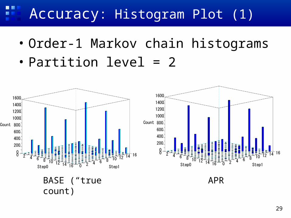
Accuracy: Histogram Plot (1)

• Order-1 Markov chain histograms

• Partition level = 2

BASE (“true” count)

APR

30

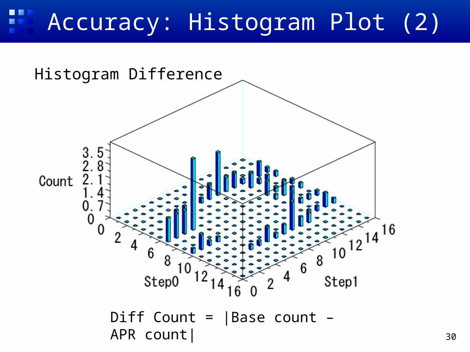
Accuracy: Histogram Plot (2)

Diff Count = |Base count – APR count|

Histogram Difference

31

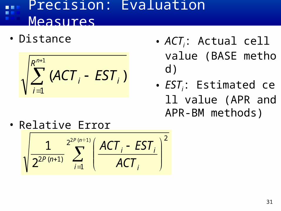
Precision: Evaluation Measures

• Distance

• Relative Error

)1(22

1

2

)1(22

1＋nP

i i

iinP ACT

ESTACT

)(1

1

nR

iii ESTACT

• ACTi: Actual cell value (BASE method)

• ESTi: Estimated cell value (APR and APR-BM methods)

32

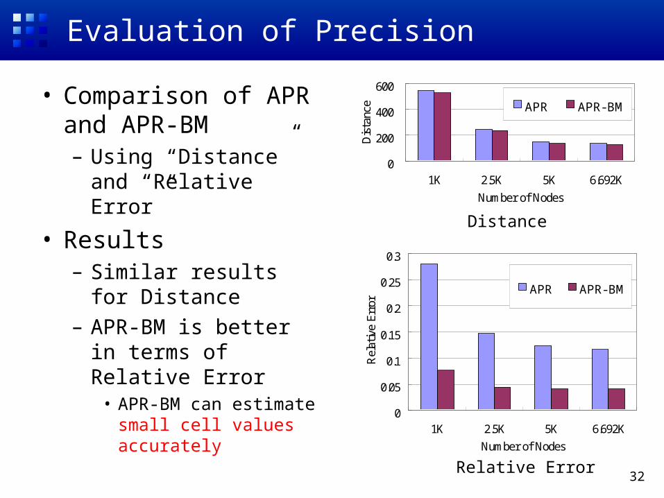
Evaluation of Precision

• Comparison of APR and APR-BM– Using “Distance” and

“Relative Error”

• Results– Similar results for

Distance– APR-BM is better in

terms of Relative Error• APR-BM can estimate

small cell values accurately

0

200

400

600

1K 2.5K 5K 6.692K

Number of Nodes

Dis

tanc

e APR APR- BM

0

0.05

0.1

0.15

0.2

0.25

0.3

1K 2.5K 5K 6.692K

Number of Nodes

Rel

ativ

e Er

ror

APR APR- BM

Distance

Relative Error

33

Outline


34

Conclusions

• Mobility histogram construction method– Based on Markov chain model– Handling streamed trajectory sequences– Logical histogram: data cube– Physical histogram: tree structure (quad tree

+ k-d tree)• Adaptive tree growth• Approximated representation method• Use of nonparametric statistics for exceptional

cases• Use of a bitmap cube to enhance precision

yoshiharu ishikawa (nagoya university) yoji machida (university of tsukuba) hiroyuki kitagawa...

Documents