120723_bachelorthesis
DESCRIPTION
thesisTRANSCRIPT

7/18/2019 120723_Bachelorthesis
http://slidepdf.com/reader/full/120723bachelorthesis 1/73
Karlsruhe Institute of TechnologyDepartment of Chemical and Process EngineeringEngler-Bunte-Institute
Division of Combustion TechnologyProf. Dr.-Ing. Henning Bockhorn
Bachelor Thesis
Implementation and Validation of a Solver
for Direct Numerical Simulations of
Turbulent Reacting Flows in OpenFOAM
by
cand. chem. ing. Henning Bonart
Evaluator: Prof. Dr.-Ing. Henning BockhornSupervisor: Dipl.-Ing. Feichi Zhang
October 2012

7/18/2019 120723_Bachelorthesis
http://slidepdf.com/reader/full/120723bachelorthesis 2/73

7/18/2019 120723_Bachelorthesis
http://slidepdf.com/reader/full/120723bachelorthesis 3/73
Karlsruher Institut für TechnologieFakultät für Chemieingenieurwesen und VerfahrenstechnikEngler-Bunte-Institut
Bereich Verbrennunsgtechnologie
Aufgabenstellung zur Bachelorarbeitcand. chem. ing. Henning Bonart
Implementierung und Validierung eines Lösers für Direkte
Numerische Simulationen von turbulenten, reagierenden
Strömungen in OpenFOAM
Ziel dieser Arbeit ist die Implementierung eines Lösers für die dreidimensionale DirekteNumerische Simulation (DNS) von turbulenten, reagierenden Strömungen in der Entwick-lungsumgebung OpenFOAM. Dabei soll die Berechnung der molekularen Flüsse auf derkinetischen Gastheorie basieren. Darüber hinaus sollen verschiedene komplexe chemischeReaktionsmechanismen eingebunden werden können.
Mittels der Simulation einer eindimensionalen, laminaren Vormischflamme soll derLöser mit Ergebnissen von CHEMKIN/PREMIX im Hinblick auf Diffusions- und Reak-tionsvorgänge validiert werden. Danach soll gezeigt werden, das dreidimensionale DNSvon turbulenten, reagierenden Strömungen mit dem Löser möglich sind. Zur Durch-führung der Simulationen soll der hauseigene Rechencluster sowie der CRAY XE6 vom
Hochleistungsrechenzentrum Stuttgart genutzt werden.
Die Arbeit gliedert sich in folgende Arbeitsschritte:1. Einarbeitung in die Theorie der turbulenten Strömung und Verbrennung2. Aussuchen eines geeigneten Lösers in OpenFOAM als Basisströmungslöser3. Erweiterung der Transportgleichungen des Basislösers auf multikomponenten Reak-
tionsmischungen4. Einbindung von Cantera zur Berechnung der Eigenschaften von multikomponen-
ten Reaktionsmischungen wie Dichte, spezifische Wärmekapazitäten, Wärmeleitko-effizient, Diffusionskoeffizienten, chemische Quellterme etc.
5. Validierung des neuen Lösers anhand einer eindimensionalen laminaren Vormis-chflamme
6. Durchführung einer dreidimensionalen DNS einer turbulenten Vormischflamme7. Beschreibung von Theorie und Implementierung sowie Darstellung und Diskussion
der Ergebnisse in einer schriftlichen Ausarbeitung8. Vorstellung der Bachelorarbeit in einem öffentlichen Seminarvortrag
Betreuer: Dipl.-Ing. Feichi ZhangAufgabensteller: Prof. Dr.-Ing. Henning Bockhorn

7/18/2019 120723_Bachelorthesis
http://slidepdf.com/reader/full/120723bachelorthesis 4/73
I declare that I have developed and written the enclosed thesis completely by myself,and have not used sources or means without declaration in the text.
Karlsruhe, October 2012 . . . . . . . . . . . . . . . . . . . . . . . . . . . . . . . . . . . . . . . . . . . . . . . . . . . . . . . . .(Henning Bonart)

7/18/2019 120723_Bachelorthesis
http://slidepdf.com/reader/full/120723bachelorthesis 5/73
ContentsFigures, Tables and Listings III
Nomenclature V
1. Introduction 11.1. Motivation . . . . . . . . . . . . . . . . . . . . . . . . . . . . . . . . . . . 11.2. Objectives . . . . . . . . . . . . . . . . . . . . . . . . . . . . . . . . . . . 31.3. Structure of the Thesis . . . . . . . . . . . . . . . . . . . . . . . . . . . . 3
2. Basic Aspects of Turbulent Combustion 52.1. Structure of Laminar Premixed Flames . . . . . . . . . . . . . . . . . . . 52.2. Characteristics of Turbulent Flow . . . . . . . . . . . . . . . . . . . . . . 7
2.2.1. Energy Cascade and Kolmogorov Scales . . . . . . . . . . . . . . 72.3. Interaction between Premixed Flames and Turbulent Flow . . . . . . . . 8
2.3.1. Turbulent Flame Speed . . . . . . . . . . . . . . . . . . . . . . . . 92.3.2. Flame Stretch Rate . . . . . . . . . . . . . . . . . . . . . . . . . . 102.3.3. Combustion Regimes . . . . . . . . . . . . . . . . . . . . . . . . . 11
3. Mathematical Description of Chemically Reacting Flows 133.1. Statistical Thermodynamics and the Rigorous Kinetic Theory . . . . . . 133.1.1. The Boltzmann Equation . . . . . . . . . . . . . . . . . . . . . . 143.1.2. Enskog’s General Transport Equation . . . . . . . . . . . . . . . . 153.1.3. Chapman-Enskog Theory . . . . . . . . . . . . . . . . . . . . . . 15
3.2. Transport Equations for Chemically Reacting Flows . . . . . . . . . . . . 163.2.1. Equations of Mass . . . . . . . . . . . . . . . . . . . . . . . . . . 163.2.2. Equation of Momentum . . . . . . . . . . . . . . . . . . . . . . . 173.2.3. Equation of Energy . . . . . . . . . . . . . . . . . . . . . . . . . . 17
3.3. Multicomponent Molecular Transport . . . . . . . . . . . . . . . . . . . . 183.3.1. Species Mass Flux . . . . . . . . . . . . . . . . . . . . . . . . . . 183.3.2. Momentum Flux . . . . . . . . . . . . . . . . . . . . . . . . . . . 203.3.3. Heat Flux . . . . . . . . . . . . . . . . . . . . . . . . . . . . . . . 21
3.4. Reaction Kinetics . . . . . . . . . . . . . . . . . . . . . . . . . . . . . . . 213.5. Chemical Time Scales . . . . . . . . . . . . . . . . . . . . . . . . . . . . 22
4. Numerical Solution of Partial Differential Equations 234.1. The Finite Volume Method . . . . . . . . . . . . . . . . . . . . . . . . . 23
4.1.1. Approximation of Integrals . . . . . . . . . . . . . . . . . . . . . . 24
I

7/18/2019 120723_Bachelorthesis
http://slidepdf.com/reader/full/120723bachelorthesis 6/73
4.1.2. Interpolation and Differentiation Procedures . . . . . . . . . . . . 254.2. Methods for Unsteady Problems . . . . . . . . . . . . . . . . . . . . . . . 264.3. Solution of Linear Equation Systems . . . . . . . . . . . . . . . . . . . . 27
5. Implemented Solver in OpenFOAM and the Cantera Interface 29
5.1. Software Packages . . . . . . . . . . . . . . . . . . . . . . . . . . . . . . . 295.2. Connection of OpenFOAM with Cantera . . . . . . . . . . . . . . . . . . 30
5.2.1. Structure of the Interface . . . . . . . . . . . . . . . . . . . . . . . 315.2.2. Integration of the Interface into OpenFOAM . . . . . . . . . . . . 315.2.3. Exchange of Data between OpenFOAM and Cantera . . . . . . . 32
5.3. Implementation of the Solver . . . . . . . . . . . . . . . . . . . . . . . . . 345.3.1. OpenFOAM’s Approach for Transport Equations . . . . . . . . . 345.3.2. Implementation of Species Mass Equations . . . . . . . . . . . . . 355.3.3. Implementation of Sensible Enthalpy Equation . . . . . . . . . . . 36
6. Validation of the Solver 376.1. Case Description . . . . . . . . . . . . . . . . . . . . . . . . . . . . . . . 376.2. Numerical conditions . . . . . . . . . . . . . . . . . . . . . . . . . . . . . 386.3. Comparison with CHEMKIN/PREMIX . . . . . . . . . . . . . . . . . . . 40
6.3.1. Temperature and Species Mass Fractions . . . . . . . . . . . . . . 406.4. Influence of the Grid Resolution . . . . . . . . . . . . . . . . . . . . . . . 426.5. Species Production Rates . . . . . . . . . . . . . . . . . . . . . . . . . . . 446.6. Computation of Chemical Time Scales . . . . . . . . . . . . . . . . . . . 44
7. Direct Numerical Simulation of a Turbulent Premixed Flame in 3D 467.1. Numerical Setup . . . . . . . . . . . . . . . . . . . . . . . . . . . . . . . 46
7.2. Initial conditions . . . . . . . . . . . . . . . . . . . . . . . . . . . . . . . 487.3. Topological Results . . . . . . . . . . . . . . . . . . . . . . . . . . . . . . 497.4. Parallel Performance of the Cray XE6 (HERMIT) . . . . . . . . . . . . . 52
8. Summary and Perspective 54
A. Code Fragments for OpenFOAM in C++3 55
B. Reaction Mechanism 57
II

7/18/2019 120723_Bachelorthesis
http://slidepdf.com/reader/full/120723bachelorthesis 7/73
Figures1.1. World energy-related C O2 emissions by scenario . . . . . . . . . . . . . . 1
2.1. Species and temperature profiles for a laminar, premixed flat methane-oxygen flame. . . . . . . . . . . . . . . . . . . . . . . . . . . . . . . . . . 6
2.2. Schematic representation of the turbulent kinetic energy spectrum E asa function of the wavenumber k . . . . . . . . . . . . . . . . . . . . . . . . 8
2.3. Kinematic interaction between a turbulent eddy and a propagating flamefront. . . . . . . . . . . . . . . . . . . . . . . . . . . . . . . . . . . . . . . 9
2.4. Schematic representation of the turbulent flame velocity. . . . . . . . . . 102.5. Schematic classification of turbulent combustion regimes. . . . . . . . . . 11
3.1. Graphical expression of the Boltzmann equation. . . . . . . . . . . . . . . 14
4.1. Parameters used in the Finite Volume Method. . . . . . . . . . . . . . . 244.2. Example of a 2D, structured, non-orthogonal grid to simulate the flow
through a duct. . . . . . . . . . . . . . . . . . . . . . . . . . . . . . . . . 254.3. Approximation of the time integral over an interval. . . . . . . . . . . . . 27
5.1. Inheritance and dependency diagram for the coupling library. . . . . . . . 32
5.2. Initialization sequence of the coupling library during runtime. . . . . . . 335.3. Data exchange between OpenFOAM and Cantera through the interface
canteraFoamModel . . . . . . . . . . . . . . . . . . . . . . . . . . . . . . . 34
6.1. Physical domain of the laminar, premixed flame. . . . . . . . . . . . . . . 386.2. Numerical domain of the laminar, premixed flame. . . . . . . . . . . . . . 396.3. Temperature and species mass fraction profiles obtained from OpenFOAM
and from CHEMKIN/PREMIX. . . . . . . . . . . . . . . . . . . . . . . . 416.4. Profiles obtained from OpenFOAM with 600 Cells and 3000 Cells. . . . . 436.5. Reaction rates obtained from OpenFOAM. . . . . . . . . . . . . . . . . . 446.6. Calculated chemical time scales τ for T , O
2 and OH . . . . . . . . . . . . 45
7.1. Numerical domain of the turbulent, premixed flame. . . . . . . . . . . . . 477.2. Initial velocity and temperature fields of the premixed turbulent flame. . 487.3. From the initial conditions calculated Kolmogorov scales. . . . . . . . . . 487.4. Isosurface of Y CH 4. Bottom with eddy dissipation rate and backside with
vorticity. . . . . . . . . . . . . . . . . . . . . . . . . . . . . . . . . . . . . 497.5. Two dimensional slices of the temperature field and the vorticity field with
heat release rate of the turbulent premixed flame. . . . . . . . . . . . . . 50
III

7/18/2019 120723_Bachelorthesis
http://slidepdf.com/reader/full/120723bachelorthesis 8/73
7.6. Different mass fractions and reaction rates. . . . . . . . . . . . . . . . . . 517.7. Scale-up on Cray XE6 with a grid of 2× 10⁶ cells. . . . . . . . . . . . . . 53
Tables
6.1. Physical conditions of the simulation with OpenFOAM. . . . . . . . . . . 376.2. Numerical setups. . . . . . . . . . . . . . . . . . . . . . . . . . . . . . . . 386.3. In OpenFOAM used discretization schemes for the mathematical terms. . 396.4. Comparison of distinctive results obtained with OpenFOAM and CHEMK-
IN/PREMIX. . . . . . . . . . . . . . . . . . . . . . . . . . . . . . . . . . 40
6.5. Comparison of distinctive results obtained with 600 Cells and 3000 Cells. 42
7.1. Physical and numerical conditions of the turbulent, premixed flame in 3D. 46
Listings
A.1. Implementation of the species equation 5.8 in OpenFOAM. . . . . . . . . 55A.2. Implementation of the energy equation 5.12 in OpenFOAM. . . . . . . . 56A.3. Initialization during run time and performing a downcast to obtain access
to derived class functions in OpenFOAM. . . . . . . . . . . . . . . . . . . 56
B.1. The used reaction mechanism in CHEMKIN format . . . . . . . . . . . . 57
IV

7/18/2019 120723_Bachelorthesis
http://slidepdf.com/reader/full/120723bachelorthesis 9/73
NomenclatureLatin symbols
∆h0f . . . . . . . . . . . . Specific standard-state heat of formation [J/kg]
D . . . . . . . . . . . . . . Binary diffusion coefficient [m2/s]M . . . . . . . . . . . . . Name [-]M . . . . . . . . . . . . . . Molecular weight [kg/kmol]A . . . . . . . . . . . . . . Surface [m2]A . . . . . . . . . . . . . Pre-exponential constant [varies]c p . . . . . . . . . . . . . . Specific heat at constant pressure [J/(kg·K)]
Co . . . . . . . . . . . . . Courant number [-]D . . . . . . . . . . . . . . Ordinary multicomponent diffusion coefficient [m2/s]d . . . . . . . . . . . . . . . Distance [m]d . . . . . . . . . . . . . . . Molecular driving force [1/m]DT k . . . . . . . . . . . . . Thermal diffusion coefficient [kg/(m·s)]
Da . . . . . . . . . . . . . Damköhler number [-]E . . . . . . . . . . . . . . Energy [J]E a . . . . . . . . . . . . . Activation energy [J/mol]F . . . . . . . . . . . . . . External force [kg·m/s2]f . . . . . . . . . . . . . . . Cell face [-]
f . . . . . . . . . . . . . . . Velocity distribution function [s
3
/m
6
]g . . . . . . . . . . . . . . . Gravitational force [kg·m/s2]H . . . . . . . . . . . . . . Terms of higher order [-]h . . . . . . . . . . . . . . . Specific enthalpy [J/kg]hc . . . . . . . . . . . . . . Specific chemical enthaly [J/kg]hs . . . . . . . . . . . . . . Specific sensible enthaly [J/kg]I . . . . . . . . . . . . . . . Total number of chemical reactions [-] j . . . . . . . . . . . . . . . Diffusive mass flux [kg/(m3·s)]K . . . . . . . . . . . . . . Total number of chemical species [-]k . . . . . . . . . . . . . . . Rate constant [varies]k . . . . . . . . . . . . . . . Wavenumber [1/m]
Ka . . . . . . . . . . . . . Karlovitz number [-]L . . . . . . . . . . . . . . . Matrix for the computation of transport quantities [-]l . . . . . . . . . . . . . . . Length [m]Le . . . . . . . . . . . . . Lewis number [-]m . . . . . . . . . . . . . . Mass [kg]N . . . . . . . . . . . . . . Number of molecules [-]n . . . . . . . . . . . . . . . Number of moles [-] p . . . . . . . . . . . . . . . Pressure [Pa]
V
7/18/2019 120723_Bachelorthesis
http://slidepdf.com/reader/full/120723bachelorthesis 10/73
Q . . . . . . . . . . . . . . Source [-]q . . . . . . . . . . . . . . . Heat flux [J/(m2·s)]r . . . . . . . . . . . . . . . Chemical reaction rate [kg/m3]Rs . . . . . . . . . . . . . Specific gas constant [J/(kg·K)]Re . . . . . . . . . . . . . Reynolds number [-]
S . . . . . . . . . . . . . . . Surface [m2]s . . . . . . . . . . . . . . . Flame speed [m/s]Sc . . . . . . . . . . . . . . Schmidt number [-]T . . . . . . . . . . . . . . Temperature [K]t . . . . . . . . . . . . . . . Time [s]T O . . . . . . . . . . . . . Inner reaction layer temperature [K]V . . . . . . . . . . . . . . Mass diffusion velocity [m/s]V . . . . . . . . . . . . . . Volume [m3]v . . . . . . . . . . . . . . . Velocity [m/s]w . . . . . . . . . . . . . . Convective or diffusive flux [-]
X . . . . . . . . . . . . . . Mole fraction [-]x, y, z . . . . . . . . . . Direction [m]Y . . . . . . . . . . . . . . Mass fraction [-]
Greek symbols
β . . . . . . . . . . . . . . . Temperature exponent [-]Γ . . . . . . . . . . . . . . . Molecular collision [-]δ . . . . . . . . . . . . . . . Thickness of inner reaction layer [m] . . . . . . . . . . . . . . . Rate of dissipation of turbulent kinetic energy [m2/s3]θ . . . . . . . . . . . . . . . Perturbation function [-]
Λ . . . . . . . . . . . . . . . Transport coefficient [-]λ . . . . . . . . . . . . . . . Air equivalence number [-]λ0 . . . . . . . . . . . . . . Thermal conductivity [W/(m·K)]µ . . . . . . . . . . . . . . . Dynamic viscosity [kg/(m·s)]ν . . . . . . . . . . . . . . . Kinematic viscosity [m2/s]ν . . . . . . . . . . . . . . . Stoichiometric coefficient [-]ξ . . . . . . . . . . . . . . . Ordering parameter [-]ρ . . . . . . . . . . . . . . . Mass density [kg/m3]σ . . . . . . . . . . . . . . . Collision diameter [m]τ . . . . . . . . . . . . . . . Stress tensor [kg/(m·s2)]
τ . . . . . . . . . . . . . . . Time scale [s]φ . . . . . . . . . . . . . . . Physical quantity [-]ψ . . . . . . . . . . . . . . . Quantity [-]Ω . . . . . . . . . . . . . . Reduced collision integral [-]ω . . . . . . . . . . . . . . . Rate of progress [kg/(m3·s)]
Indices and Accents
0 . . . . . . . . . . . . . . . U n b u r n t
VI

7/18/2019 120723_Bachelorthesis
http://slidepdf.com/reader/full/120723bachelorthesis 11/73
¯ . . . . . . . . . . . . . . . Mean v al ue† . . . . . . . . . . . . . . . Transposed˙ . . . . . . . . . . . . . . . Time derivation/rate∞ . . . . . . . . . . . . . . Surrounding . . . . . . . . . . . . . . . Vector
c . . . . . . . . . . . . . . . Characteristici . . . . . . . . . . . . . . . Species ik . . . . . . . . . . . . . . . S p e c i e s kL . . . . . . . . . . . . . . . L a m i n a rT . . . . . . . . . . . . . . Turbulent
Constants . . . . .kB . . . . . . . . . . . . . Boltzmann constant (1.3806488·10−23) [J/K]N A . . . . . . . . . . . . . Avogadro constant (6.02214129·1023) [mol−1]R . . . . . . . . . . . . . . Universal gas constant (8.3144621) [J/(mol
·K)]
Abbreviations
1D . . . . . . . . . . . . . One dimension3D . . . . . . . . . . . . . Three dimensions fvc . . . . . . . . . . . . . finite volume calculus fvm . . . . . . . . . . . . finite volume methodCFD . . . . . . . . . . . Computational Fluid DynamicsBLAS . . . . . . . . . . Basic linear algebra subprogramsCFL . . . . . . . . . . . . Courant–Friedrichs–Lewy conditionCG . . . . . . . . . . . . . Conjugate gradients
CHEMKIN . . . . . Software for chemical kineticsDNS . . . . . . . . . . . Direct numerical simulationFDM . . . . . . . . . . . Finite Difference MethodFVM . . . . . . . . . . . Finite Volume MethodGPL . . . . . . . . . . . General Public LicenseLAPACK . . . . . . . Linear algebra packageLES . . . . . . . . . . . . Large eddy simulationLU . . . . . . . . . . . . . Lower upperMATLAB . . . . . . Matrix laboratoryMPI . . . . . . . . . . . . Message Passing Interface
MPI . . . . . . . . . . . . Message passing interface, e.g. MPICH2/OpenMPINRBC . . . . . . . . . Non-reflecting boundary conditionsODE . . . . . . . . . . . Ordinary differential equationOpenFOAM . . . . Open Source Field Operation and Manipulation, registered trademark
of OpenCFD LimitedPBiCG . . . . . . . . . Preconditioned biconjugated gradientPCG . . . . . . . . . . . Preconditioned conjugate gradientPDE . . . . . . . . . . . Partial differential equation
VII

7/18/2019 120723_Bachelorthesis
http://slidepdf.com/reader/full/120723bachelorthesis 12/73
PISO . . . . . . . . . . . Pressure implicit with split operatorRANS . . . . . . . . . . Reynolds-averaged Navier–StokesSIMPLE . . . . . . . Semi-implicit method for pressure-linked equationsSUNDIALS . . . . Suite of nonlinear and differential/algebraic equation solvers
VIII

7/18/2019 120723_Bachelorthesis
http://slidepdf.com/reader/full/120723bachelorthesis 13/73
1. Introduction1.1. Motivation
Chemically reacting flows impact many aspects of human life via, for example, medicinalchemistry, chemical synthesis, material processing and combustion processes [1]. Com-bustion of hydrocarbon fossil fuels (or fuels stemming from renewable sources) is still animportant part of almost every energy conversion [2].
Technical applications based on combustion processes are important for transportation,
power generation and chemical engineering. At the same time pollution caused bycombustion processes leads to environmental problems. For instance, the contributionof CO2 emissions to global warming is now considered to be proven and may be amain threat to our standard of living. Figure 1.1 shows the world-energy related CO2
emissions by different scenarios. To reach the 450 Scenario1 an improvement of directand indirect energy conversion efficiency is without alternative [2].
Fig. 1.1.: World energy-related C O2 emissions by scenario. Figure taken from [2].
Other pollutants, such as unburnt hydrocarbons, soot, nitrogen oxides and sulfur ox-ides, can contribute to health hazards and cause smogs or acid rain [3]. However, due tostricter government regulations for, e.g., the automotive industry and the energy sector,pollutants emission has been reduced. In order to be conform to such legal regulations
1The 450 Scenario describes pathways to a long-range CO2 concentration in the atmosphere of 450parts per million, see [2].

7/18/2019 120723_Bachelorthesis
http://slidepdf.com/reader/full/120723bachelorthesis 14/73
1.1. MOTIVATION 2
and to meet the public expectation about cleaner and more efficiently industrial pro-cesses as well as to reach the 450 Scenario target of the Internal Energy Agency, it isstill of crucial importance to improve combustion technology.
Since most of the industrial applications of combustion involve turbulent flows, a deeper
understanding of the interplay between turbulence and combustion is needed. In manycases turbulence increases combustion. On the other hand the heat release leads to gasexpansion and density variations and therefore influences the turbulent flow [4]. Thisinteraction of turbulence and chemical reaction is still not fully understood. Due to thesmall length and time scales, details of the mixing process, as well as the structures inturbulent flows, have not been fully investigated, yet. Therefore, a deeper understandingof the interplay between turbulence and chemical reaction processes is of large interestin order to improve efficiency in combustion.
The mechanisms involved in such turbulent combustion flows have been the object of
numerous theoretical, experimental and numerical scientific research in the last cen-tury [4–6]. Thereby, experimental studies have greatly advanced our knowledge on tur-bulent combustion. Recently, experiments that simultaneously measured the turbulentvelocity fields and the reacting scalar concentrations, together with the local temper-ature, have contributed to a more realistic understanding of such turbulent burningprocesses. However, in order to gain detailed insight into the fundamental physics of theturbulence-chemistry interaction on small space and time scales, numerical simulationsare to date without alternative.
In numerical simulations of turbulent combustion, additionally to the standard com-
plexities of turbulent non-reacting simulation, other difficulties, such as the strong heatrelease and the complex chemistry behind the combustion process, have to be takeninto account [7]. The computational grid has to be sufficient small in order to resolvethe smallest eddies in the turbulent flow. Due to numerical stability reasons very smalltime steps are necessary. Hence, direct numerical simulations of turbulent reacting flowsdemand a prohibitive amount of computational time. However, the huge progress incomputer technology in the past two decades now offers the opportunity for direct nu-merical simulations of three-dimensional (3D) turbulent reacting flows for certain cases.This allows for studying the chemistry-turbulence interaction in more detail (see e.g. [8,9]).
For a direct numerical simulation the underlying physical and chemical models whichdescribe chemical kinetics or molecular transport are required to be as precise as possible.Thanks to extensive research in chemical kinetics a lot of chemical mechanisms can nowbe modeled with great precision. Consequently, highly realistic chemical kinetic modelsare implemented in many fluid dynamics codes. However, the use of multicomponenttransport equations based on the Maxwell-Stefan diffusion model or the rigorous kinetictheory of ideal gases is still rare in computational fluid dynamics. The reason is probablythe additional complexity of the implementation and the higher computational cost.Numerous studies have shown that, when omitting multicomponent diffusion equations,significant errors occur in simulations of laminar flames [1, 10–13]. As to turbulent flow,

7/18/2019 120723_Bachelorthesis
http://slidepdf.com/reader/full/120723bachelorthesis 15/73
1.2. OBJECTIVES 3
scientific publications comparing different diffusion models are very rare but it has beenargued by [9, 14] that accuracy should be improved when using the full multicomponenttransport equations.
1.2. ObjectivesIn the present thesis the main objective is to implement and validate a DNS solver whichis able to simulate turbulent, chemically reacting flows with a detailed diffusion modelingand complex chemical kinetics. The equations are implemented with as little simplifica-tions as possible and mostly derived from the rigorous kinetic theory of gases. The C++toolbox OpenFOAM is used as the underlying structure for the DNS solver. The mainadvantages of OpenFOAM are its high numerical accuracy and its free availability [15].
Moreover, multicomponent transport coefficients, which are obtained from the extendedChapman-Enskog theory [16] and based on the molecular properties of the gases, areused. These multicomponent diffusion coefficients are calculated with Cantera, an opensource chemical kinetics software. Cantera features a high calculation speed when calcu-lating chemical source terms based on complex chemical mechanisms as well as efficientcalculation routines for multicomponent coefficients [17]. The interconnection betweenOpenFOAM 2.0.1 and Cantera is newly programmed based on an library by [18] forOpenFOAM 1.5.
To validate the solver laminar premixed flames are simulated and compared to cal-culations obtained with CHEMKIN/PREMIX with respect to numerical accuracy andstability. Furthermore, the simulation of a turbulent premixed flame in 3D is carried
out. For that purpose, the solver, as well as the OpenFOAM framework and the Canteraroutines, are adapted for the hardware structure of the high performance cluster CrayXE6 in Stuttgart, Germany, where the simulations have been carried out.
1.3. Structure of the Thesis
The thesis is organized in the following way: After the current introduction a generaldiscussion on the physics of the combustion and flow dynamics in chapter 2 is presented.In the following chapter 3 the mathematical description of chemically reacting flows ispresented with an introduction to statistical thermodynamics and the kinetic theory of gases, from which the transport equations, as well as the equations for the molecularfluxes are derived. A brief discussion of chemical kinetics follows, to close the mathemat-ical description of the partial differential equations. The organization of the thesis fromsections 3.1 to 3.4 has been designed in a way to gradually guide the reader from themost basic physical model as a starting point towards the later implemented equations.The numerical methods used in the simulation of reacting flows are presented in chapter4. The finite volume method is discussed, as well as methods for unsteady problemsand solution strategies for linear equation systems. Chapter 5 gives at first an overviewover the used software. In the following, the coupling library between OpenFOAM and

7/18/2019 120723_Bachelorthesis
http://slidepdf.com/reader/full/120723bachelorthesis 16/73
1.3. STRUCTURE OF THE THESIS 4
Cantera is presented and the new solver for DNS of chemically reacting flows with multi-component diffusion modeling is introduced. In chapter 6 the developed solver is appliedto numerical simulations of flat premixed flames for validation purpose. The results arecompared with calculations obtained from CHEMKIN/PREMIX. Finally the solver isused for DNS of 3D turbulent premixed flames and the results are briefly discussed in
chapter 7. The thesis finishes with a conclusion and a perspective.

7/18/2019 120723_Bachelorthesis
http://slidepdf.com/reader/full/120723bachelorthesis 17/73
2. Basic Aspects of TurbulentCombustion
Combustion is a highly exothermic, chemical reaction between a fuel and an oxidizer.There are two general types of combustion processes which can be distinguished by thenature of their mixing state. In a premixed combustion the composition of fuel andoxidizer is spatially homogeneous while in a non-premixed combustion the unburnt fuelcomposition varies in space such that mixing and chemical reaction occur simultane-ously. Between these two extremes one often encounters so called partially-premixed
flames. Secondly, combustions may be classified with respect to the underlying flowregimes which can be either laminar or turbulent. Latter is encountered in most practi-cal combustion systems such as combustion engines, aircraft engines, industrial burnersand furnaces.
In the following sections a brief description of the different flame types with respect totheir mixing state and fluid motion is presented and some fundamental definitions areintroduced.
2.1. Structure of Laminar Premixed FlamesA flow is defined laminar if the fluid layers move smoothly in such a way that they remainordered and do not mix in the plane perpendicular to the direction of the flow [19].Whether a flow is laminar or not depends on the ratio of the inertial and viscous forceswhich is used to define the Reynolds number
Re = lcvρ
µ , (2.1)
where lc is a characteristic length, v is the flow velocity, ρ is the mass density and µis the dynamic viscosity. If a critical value of Re is reached the laminar flow starts tobecome unstable and changes to turbulent flow. For example in an internal channel flow,this happens at Re ≈ 2000.
Laminar premixed flames propagate towards a premixed mixture of fuel and air. Theyoccur in gas ranges, heating appliances and Bunsen burners. The understanding of laminar premixed flames is a prerequisite to study turbulent premixed flames [10]. Dueits simple configuration laminar premixed flat flames have been an important objectin numerical combustion science. Therefore a lot of specialized numerical codes, likeCHEMKIN/PREMIX [20] and Cantera [17], exist.

7/18/2019 120723_Bachelorthesis
http://slidepdf.com/reader/full/120723bachelorthesis 18/73
2.1. STRUCTURE OF LAMINAR PREMIXED FLAMES 6
Fig. 2.1.: Species and temperature profiles for a laminar, premixed flat methane-oxygen flame. Figuretaken from [4].
In order to distinguish different mixtures of fuel and oxidizer the air number is definedas [10]
λair = X air/X fuel
X air,stoich./X fuel,stoich. , (2.2)
where X air (X fuel) are the mole fractions of the air (fuel) in the mixture, and X air,stoich.(X fuel,stoich.) are the mole fractions of the air (fuel) in the stoichiometric mixture. Basedon the value of λair premixed combustions can be divided into different classes: richcombustion with λair < 1, stoichiometric combustion with λair = 1 and lean combustionwith λair > 1.
The schematic structure of a premixed, flat, methane-air flame is shown in Figure 2.1.It consists of three main regions. In the chemically inert preheating zone, heat released
from the reaction is transported by conduction. The reaction layer is typically thin andcalled fuel consumption layer or inner layer with thickness δ and temperature T O. Thislayer is responsible for keeping the reaction process alive. Here the fuel is consumed andthe radicals are depleted by chain-breaking reactions. The inner layer temperature T Ocorresponds to the crossover temperature between chain-branching and chain-breakingreactions. In the oxidation layer the final oxidation to the products is accomplishedand the temperature reaches its maximum. The thickness of the reaction zone δ can becalculated from the temperature profile with [21]
δ = T 2 − T 1
max ∂T ∂x . (2.3)

7/18/2019 120723_Bachelorthesis
http://slidepdf.com/reader/full/120723bachelorthesis 19/73
2.2. CHARACTERISTICS OF TURBULENT FLOW 7
In a steady flow of premixed gas, the flame propagates upstream until the flow velocitynormal to the flame front is equal to the laminar flame speed sL. The laminar flamespeed can be calculated from the integral of the burning rate across the flame brushwith [21]
sL
=−
1
ρ0Y fuel,0 +∞
−∞rfuel
dx . (2.4)
The laminar burning velocity dependence on the fuel type, the air number, the pres-sure, the unburnt flow temperature, etc. and is a very important characterization of combustions [4].
2.2. Characteristics of Turbulent Flow
As mentioned in the section before the occurrence of turbulent flow essentially dependson the ratio of inertial and viscous forces in the fluid. In a turbulent flow the destabi-
lizing inertial forces exceed the stabilizing viscous forces such, that the generation rateof vortices is higher then the viscous dissipation rate [19]. Therefore, turbulence arisesfrom instabilities associated with large Re numbers.
To further characterize the flow, a turbulent Reynolds number ReT is introduced [22]:
ReT = vlT
ν (2.5)
Here, v is the turbulence intensity or velocity fluctuation, ν is the kinematic viscosityand lT is the turbulent length scale. The turbulent Reynolds number represents the
ratio of turbulent transport to molecular transport of momentum.
Compared to laminar flows, turbulent flows have no well-defined values for velocities andphysical scalars. The flow regime is characterized by transient chaotic and stochasticproperty changes. Variations of velocity lead to fluctuations in physical scalars such asdensity, temperature or transport quantities. Since the physics of turbulence are notfully understood the integration of chemical reactions is even more difficult.
2.2.1. Energy Cascade and Kolmogorov Scales
Turbulence can be considered to be composed of eddies of different sizes. Large eddiesare unstable and break up, transferring their energy E to somewhat smaller eddies whichbreak up again. This energy cascades continuous until the Reynolds number of the eddyis sufficiently small that the eddy motion is stable and molecular viscosity is effective indissipating the kinetic energy [22].
Figure 2.2 shows the energy spectrum measured for all wavelengths k. For smallwavenumbers corresponding to large scale eddies the energy per unit wavenumber in-creases with a power law between k2 and k4 . This range is not universal and is deter-mined by large scale instabilities, which depend on the boundary conditions of the flow.The spectrum attains a maximum at a wavenumber that corresponds to the integral or

7/18/2019 120723_Bachelorthesis
http://slidepdf.com/reader/full/120723bachelorthesis 20/73
2.3. INTERACTION BETWEEN PREMIXED FLAMES AND TURBULENT FLOW 8
Fig. 2.2.: Schematic representation of the turbulent kinetic energy spectrum E as a function of thewavenumber k.
turbulence macroscale l0, since eddies of that scale contain most of the kinetic energy.For larger wavenumbers corresponding to the inertial sub-range the energy spectrum de-creases following the k−5/3 law. Finally, there is a cutoff at the Kolmogorov microscalelK . In the viscous sub-range, the energy per unit wavenumber decreases exponentiallyowing to viscous effects. Therefore, the Kolmogorov microscale represents the smallest
length scales associated with a turbulent flow [4].
To determine the necessary grid resolution and time step in numerical simulations of turbulent flows one has to know about the value of the smallest scales. The Kolmogorovmicroscale for length lK and time τ K are defined in [22] to
lK = (ν 3/)1/4 and τ K = (ν/)1/2 , (2.6)
in which is the rate of dissipation of turbulent kinetic energy defined to
= 2ν
sijsij
= ν
∂vi
∂x j+
∂v j
∂xi∂vi
∂x j+
∂ v j
∂xi , (2.7)
and ν is the kinematic viscosity. Here, sij is the fluctuating strain rate and is theexpectation.
2.3. Interaction between Premixed Flames and
Turbulent Flow
A highly exothermic chemically reaction and turbulence can have large influences on eachother. The flow is strongly accelerated by passing the flame front due to the thermal

7/18/2019 120723_Bachelorthesis
http://slidepdf.com/reader/full/120723bachelorthesis 21/73
2.3. INTERACTION BETWEEN PREMIXED FLAMES AND TURBULENT FLOW 9
expansion. In addition, turbulent eddies wrinkle the flame front (as illustrated in figure2.3) and enhance the chemical reaction. In some cases on the other hand, the flow cancompletely inhibit the chemical reaction and lead to flame quenching [4].
Fig. 2.3.: Kinematic interaction between a turbulent eddy and a propagating flame front.
2.3.1. Turbulent Flame Speed
Unlike the laminar flame speed, which depends mostly on the thermal and chemicalproperties of the unburnt mixture, the turbulent flame speed sT also depends on thetransient interaction between turbulence and chemical reaction. As shown in figure 2.4the instantaneous flame front represents a large area AT propagating with the locallylaminar flame speed sL. One can see, that the turbulent flame front is much greater thanthe mean flame area AT
A. For an observer traveling with the flame, the turbulent
flame speed can be defined as the velocity at which reactants enter the flame zone in adirection normal to the flame. Thus, the turbulent flame speed can be expressed as
m = ρ0AT sL = ρ0 AsT , (2.8)
with m equal the mass flow rate of the unburnt gas mixture and ρ0 equal the unburntmixture mass density. Consequently the ratio of turbulent flame speed to local laminarflame speed is equal to the ratio of wrinkled flame area to the mean flame area fromwhich sT can be calculated to
sT
sL
= AT
¯A →
sT = AT
¯A
sL . (2.9)

7/18/2019 120723_Bachelorthesis
http://slidepdf.com/reader/full/120723bachelorthesis 22/73
2.3. INTERACTION BETWEEN PREMIXED FLAMES AND TURBULENT FLOW 10
In addition, the turbulent burning velocity can be calculated with
sT = − 1
Aρ0Y fuel,0
+∞
−∞rFl dV , (2.10)
which is similar to equation (2.4) for the laminar burning velocity.
Fig. 2.4.: Schematic representation of the turbulent flame velocity. Figure similar to [4].
2.3.2. Flame Stretch Rate
The flame stretch rate is an important quantity in the understanding of flame phenomenasuch as extinction and the local structure of turbulent flames. In general, the flame
stretch rate reads [21]κ =
1
AT
dAT dt
, (2.11)
which describes the fractional rate of change of a flame surface element AT . Note, thatthis equation uses the substantial derivation of the surface to include the convectivechange. Because of the highly unsteady flame surface, AT can not be easily calculated.Therefore, different approaches for equation (2.11) have been developed (see e.g. [23]).Here, an expression for the flame stretch rate of stoichiometric premixed flames is derivedbased on chemical reaction rates. Assuming, that the total inlet mass of reactants isconsumed by chemical reactions with rate r in the flame volume V Fl. and taking equation(2.8) into account, one can write
mfuel = V Fl.
rfuel(V ) dV = ρ0Y fuel,0AT sL = ρ0Y fuel,0 AsT . (2.12)
With A = const., sL = const. and ρ0 = const. it must apply, that
sT ∼ AT ∼ V Fl.
rfuel(V ) dV ≈i
rfuel,iV i = V CV i
rfuel,i , (2.13)
with V CV as the volume of a single cell which is equal for all cells in an equidistant mesh.Consequently, it must apply locally in cell i, that
(sT )i ∼
(AT )i ∼
V CV (rfuel)i . (2.14)

7/18/2019 120723_Bachelorthesis
http://slidepdf.com/reader/full/120723bachelorthesis 23/73
2.3. INTERACTION BETWEEN PREMIXED FLAMES AND TURBULENT FLOW 11
Finally, by inserting the expressions in equation (2.11) the flame stretch rate κ can beexpressed as
κ = 1
AT
dAT dt
= 1
rfuel
drfueldt
. (2.15)
This equation describes the fractional rate of change of the fuel consumption rate rfuel.Note, that this equation is valid for every reactant.
2.3.3. Combustion Regimes
Diagrams defining regimes of premixed turbulent combustion in terms of velocity andlength scale ratios have been proposed by many authors (see e.g. [4] for details). Here, aregime diagram, figure 2.5, is discussed following [21]. Therefore, two additional reducednumbers are used, the turbulent Damköhler number DaT and the Karlowitz number K a,defined as:
DaT = τ T τ c= lT /v
δ/sL(2.16)
Ka = τ c
τ K =
δ 2
l2K
(2.17)
DaT describes the ratio between the turbulent time scale τ T and the characteristic chem-ical time scale τ c. The interaction of the chemical reaction with the dissipative turbulentstructures of the flow field is described with K a, which is the ratio of the characteristicchemical time scale and the characteristic time scale of the smallest Kolmogorov eddyτ K . Additionally, the turbulent Reynolds number introduced before is used in the dia-gram 2.5.
Fig. 2.5.: Schematic classification of turbulent combustion regimes.

7/18/2019 120723_Bachelorthesis
http://slidepdf.com/reader/full/120723bachelorthesis 24/73
2.3. INTERACTION BETWEEN PREMIXED FLAMES AND TURBULENT FLOW 12
By using the reduced numbers ReT , K a and Da, turbulent premixed combustions can beclassified into three major categories. The thin reaction zone regime or flamelet regimeexists for K a < 1, which means, that the flame thickness is smaller than the Kolmogorovlength scale. It assumes, that the flame structure is not effected by turbulence. Theflame sheet is wrinkled by vortices not small enough to enter it. At Da > 1 and K a > 1,
the smallest eddies can enter into the flame front and enhance the diffusion inside of theflame, which leads to a thickened flame. Here, the turbulent flow is intense enough togenerate eddies able to effect the structure of the reaction zone. Since it is expected,that the lifetime of such eddies is very short, their impact on the reaction zone is thuslimited. If the reaction time is greater than the time needed for turbulent fluctuation,a well stirred reactor regime occurs. It is characterized by Da < 1 and Ka > 1.Consequently, most of the eddies can enter into the reactive-diffusive layer during theirlifetime and enhance the diffusivity within the reaction zone. It is even possible, thatnearly all of the eddies are embedded into the reaction zone. Hence, the flame front isvery thick and behaves similar to an ideally stirred reactor. Since in a turbulent flow a
wide range of length scales occur, a turbulent premixed flame is not represented by asingle point in figure 2.5, but by a zone that may cross the different regimes.

7/18/2019 120723_Bachelorthesis
http://slidepdf.com/reader/full/120723bachelorthesis 25/73
3. Mathematical Description ofChemically Reacting Flows
In the following an introduction to statistical thermodynamics and the rigorous kinetictheory of gases (see [1, 24, 25]) is presented. The focus in this section is on the Chapman-Enskog formulation and will not go through detailed derivations of all results. After,the transport equations, as well as the equations for the molecular fluxes are derivedfrom the Chapman-Enskog formulation. A brief discussion of chemical kinetics follows,to close the mathematical description of the partial differential equations.
3.1. Statistical Thermodynamics and the Rigorous
Kinetic Theory
Statistical thermodynamics apply probability theory to a large number of particles in or-der to add a molecular-level interpretation of the macroscopic thermodynamic quantitiesdescribed by classical thermodynamics. It therefore provides a mathematical descriptionof thermodynamic, chemical kinetic and transport quantities which are needed in thenumerical simulation of chemically reacting flows [24].
The rigorous kinetic theory of gases is used to relate the motion or kinetic energy of a large number of molecules to macroscopic thermodynamic quantities [1]. The theorymakes the assumptions that
(i) only binary collisions occur and that therefore the pressure of the gas mixture ismoderate
(ii) quantum-mechanical effects are negligible and that therefore temperature has tobe moderate
(iii) the dimensions of the containing vessel and any obstacle therein are large comparedto the molecule mean free path which means that the average distance separatingthe gas particles is large compared to their size.
Strictly speaking, the rigorous kinetic theory of gases applies only for elastic collisionsbut it can be extended to take account for the effect of inelastic collisions.
Since the assumptions made by the rigorous kinetic theory include the properties for anideal gas the equation of state is given by
pV = N kBT = nN AkBT = nRT (3.1)
where p is the pressure, V is the volume, N is the number of molecules, kB the Boltzmannconstant, T the temperature, n the number of moles, N A is the Avogadro constant andR is the universal gas constant.

7/18/2019 120723_Bachelorthesis
http://slidepdf.com/reader/full/120723bachelorthesis 26/73
3.1. STATISTICAL THERMODYNAMICS AND THE RIGOROUS KINETIC THEORY 14
3.1.1. The Boltzmann Equation
The Boltzmann equation given by [26] or [25]1 is used as a starting point:
∂f k
∂t
+ vk
·
∇f k +
1
mk F k
·
∂ f k
∂vk = j Γ(+)
kj
−Γ(−)kj (3.2)
As shown in figure 3.1, equation (3.2) describes the time evolution of the velocity dis-tribution function f k(x, vk, t). The quantity f k(x, vk, t)dxdvk is the mean number of molecules of species k at time t, which are located in the volume element dx around x,and which have velocities within the range dvk around vk. The population of moleculespropagating to a different position in phase space after a time dt is increased by somecollisions Γ
(+)kj and decreased by others Γ
(+)kj . The Γkj involve the intermolecular poten-
tial energy function, e.g. the Lennard-Jones-Potential, and all details of the collisiontrajectories [19]. The quantity F k is an external force acting on a molecule of species k .
Fig. 3.1.: Graphical expression of the Boltzmann equation.
The Boltzmann equation can be viewed as a transport equation in the six-dimensionalposition-velocity space, where the right hand side of equation (3.2) serves as a sourceterm. In cases where the function f can be calculated all properties of a gas mixture,like its local temperature of the chemical properties are completely known [ 19].
1Different from [25] from now vector-tensor notation is used, e.g. [19]

7/18/2019 120723_Bachelorthesis
http://slidepdf.com/reader/full/120723bachelorthesis 27/73
3.1. STATISTICAL THERMODYNAMICS AND THE RIGOROUS KINETIC THEORY 15
In the following subsections, the Boltzmann equation is used to derive the transportequations for mass, momentum and energy, as well as formulations for the molecularfluxes and the transport properties.
3.1.2. Enskog’s General Transport Equation
A general transport equation for a physical quantity can be derived from the Boltzmannequation without actually determining the form of the distribution functions f k. Bymultiplying equation (3.2) with the quantity ψk of species k and by integrating over vkone obtains Enskog’s general transport equation for the physical quantity ψk associatedwith the i-th kind of molecule [25]
∂ (nkψk)
∂t + ∇ · (nkψkvk)−nk
∂ψk
∂t +
vk · ∇ψk
+
F k
mk
· ∂ ψk∂vk
=
ψk j Γ(+)kj
−Γ
(−)kj dvk ,
(3.3)
where nk is the number of moles of species k and where the overbars indicate averagedquantities. A summation of equation (3.3) over all species k gives the transport equationfor quantity ψ of the entire gas mixture.
For conserved quantities, such as momentum (ψ = k mkvk), kinetic plus internal energy
(ψ = k
12
mkv2k + e(int)
k ) or the global mass (ψ = k mk) it is explicitly shown in [25],
that the right hand side of equation (3.3) vanishes as it should. Note that, however, thatthe mass of one species k is not conserved in case of a chemical reaction: By choosingψk = mk the sum of the right hand side of equation (3.3) represents the conversion rateof molecules of species k which is in general not zero.
In section 3.2 Enskog’s general transport equation (3.3) is used to derive explicit formu-lations for the transport equations of mass, momentum and energy.
3.1.3. Chapman-Enskog Theory
To obtain rigorous expressions for the molecular fluxes and the corresponding transportcoefficients a solution to the Boltzmann equation (3.2) has to be found. Here, a practi-cal solution given by Enskog is presented [26]. By expanding the velocity distribution
function f k with different orders of approximation f [r]k one obtains
f k = f [0]k + ξf [1]
k + ξ 2f [2]k + · · · ξ rf [r]
k ; , (3.4)
with ξ as an ordering parameter. One can find an analytical solution for the 0-thapproximation of f k [25]. Now the first-order approximation to f k can be written interms of a perturbation function θk as
f [1]k = f
[0]k θk , (3.5)
and substitute f [1]k in equation (3.2) to obtain an integro-differential equation for θ. As
shown by [25], θ has a specific form with two unknown scalar functions [1]. By expanding

7/18/2019 120723_Bachelorthesis
http://slidepdf.com/reader/full/120723bachelorthesis 28/73
3.2. TRANSPORT EQUATIONS FOR CHEMICALLY REACTING FLOWS 16
the unknown scalar functions in finite series of Sonine polynomials, one can use theresults to obtain first-order approximations of the molecular fluxes and the transportproperties [25]. Approximations of higher order are not worthwhile since the calculationis very time consuming and the additionally gained accuracy is small [16].
3.2. Transport Equations for Chemically Reacting
Flows
For numerical simulation of chemically reacting flows the transport equations constitutethe mathematical and physical core of the simulation. Here, the transport equationsare presented in a different way from the traditional continuum mechanics approach,e.g. [19]. Following [25], it is shown, that, based on the Boltzmann equation respectivelyEnskog’s general transport equation presented before, the equations of mass, momentumand energy are direct consequences of the conservation laws for mass, momentum and
energy.
Generally, a transport equation can be written as
∂
∂t(ρφ)
Transient term
= − ∇ · (ρvφ) Convection term
− ∇ · (Λφ ∇φ) Diffusion term
+ Qφ Source term
, (3.6)
with the conserved quantity φ and transport coefficient Λφ. The transient term accountsfor the accumulation of φ and the source term represents any sources or sinks in theconcerned control volume. The fluxes over the control volume faces are described by
either the convective term due to the flow velocity field v or the diffusion term due toits gradients.
3.2.1. Equations of Mass
By choosing ψk = mk in equation (3.3) one obtains, after some intermediate transfor-mations, the transport equation of the mass fraction for each species k in a mixture of K species [25]
∂
∂t(ρY k) = − ∇ · (ρY kv)− ∇ · jk + rk k = 1, 2, 3, · · · , K , (3.7)
where Y k = mk/m is the mass fraction of k-th species, ρ is the mixture density, v isthe velocity, rk is the reaction rate of species k (see section 3.4) and jk is the moleculardiffusion flux (see section 3.3).
Summing equation (3.7) over all Y k and using the relations
N k=1
Y k = 1,N k=1
jk = 0,N k=1
rk = 0 (3.8)

7/18/2019 120723_Bachelorthesis
http://slidepdf.com/reader/full/120723bachelorthesis 29/73
3.2. TRANSPORT EQUATIONS FOR CHEMICALLY REACTING FLOWS 17
one obtains the transport equation for the total mass of a multicomponent reactingmixture [19, 25]
∂ρ
∂t = − ∇ · (ρv) . (3.9)
3.2.2. Equation of MomentumThe momentum of a system of two colliding molecules is always conserved in any colli-sion, even if a chemical reaction occurs. By choosing ψk = mkvk in equation (3.3) oneobtains the equation of momentum with gravitation g as the only external force as [25]
∂
∂t(ρv) = − ∇ · (ρvv)− ∇π + ρg , (3.10)
where ∇π = ∇ p + ∇ · τ (3.11)
is the rate of momentum addition by molecular transport with τ as the molecular mo-mentum flux vector (compare section 3.3).
3.2.3. Equation of Energy
Applying ψk = 12
mkv2k + u
(int)k into equation (3.3) and summing over all species k one
obtains the transport equation for energy. By using the thermodynamic definition of enthalpy the transport equation for specific enthalpy is given as [1, 25]
∂
∂t(ρh) = − ∇ · (ρhv)− ∇ · q − τ : ∇v +
D p
Dt + Qsource , (3.12)
where q is the molecular heat flux (compare section 3.3), Qsource is a combination of all heat source terms like the radiative flux, D p
Dt is the reversible rate of enthalpy due
to compression and (τ : ∇v) is the irreversible rate of enthalpy due to viscous dissipation.
Further with the sensible enthalpy hs and the chemical enthalpy hc the total enthalpyh can be expressed as [21]
h = hs + hc = T T 0
c p(T ) dT
sensible enthalpy
+N k=1
∆h0f,kY k
chemicalenthalpy
, (3.13)
with the heat capacity for an ideal gas at constant pressure [24]
c p(T ) =
∂h
∂T
p
. (3.14)
Neglecting viscous dissipation and heat source terms like the radiative flux, one obtainsthe equation of energy in terms of sensible enthalpy to
∂
∂t
(ρhs) =
−
∇ ·(ρhsv)
−
∇ · q +
D p
Dt
+ q reaction . (3.15)

7/18/2019 120723_Bachelorthesis
http://slidepdf.com/reader/full/120723bachelorthesis 30/73
3.3. MULTICOMPONENT MOLECULAR TRANSPORT 18
The separation of sensible enthalpy from the heat of formations gives this equation theadvantage over equation (3.12), that the heat of formations become the only source term
q reaction = −N
k=1
∆h0f,k rk . (3.16)
Additionally, this equation can be used as a definition for the heat release rate.
To obtain the temperature from the sensible enthalpy, the definition of the sensibleenthalpy (3.13) is solved for T . In general, the mixture averaged specific heat cP (T ) =K k=1 c p,k(T )Y k is a function of T and therefore, the integral in (3.13) has to be solved
iteratively [21]. The temperature dependencies of the pure species specific heat capacitiesc p,k are fitted by 4-th order NASA polynomials:
c p,k(T ) M k
R
= a1,k + a2,kT + a3,kT 2 + a4,kT 3 + a5,kT 4 (3.17)
Here, an,k are coefficients of the k-th species which has to be given as input.
3.3. Multicomponent Molecular Transport
Gradients exist in a gas under non-equilibrium conditions in one or more physical quan-tities: composition, mass averaged velocity and temperature. These gradients cause themolecular or diffusive transport of mass, momentum and energy through the gas.
In this section, expressions for the diffusive flux vectors in the transport equations (3.7),(3.10) and (3.15) will be derived based on the Chapman-Enskog formulation in subsection3.1.3. In addition, a formulation for multicomponent transport coefficients laid outby [16] for computational purpose will be given.
3.3.1. Species Mass Flux
Inserting the first approximation of the distribution function in terms of the perturbationfunction mentioned in subsection 3.1.3 and making use of the polynomial expansions andorthogonality relations [25] one obtains the mass diffusion velocity [1, 16]
V k = 1X kM
N j=1
M jDkj d j − DT kρY k
1T
∇T , (3.18)
where X k = nk/n is the molar fraction of species k, M is the mean molecular weight, M jis the molecular weight of species j, Dkj is the ordinary diffusion coefficient of speciesk through species j, DT k is the thermal diffusion coefficient of species k and the driving
force d j is defined as
d j = ∇X j + (X j − Y j)1
p ∇ p . (3.19)

7/18/2019 120723_Bachelorthesis
http://slidepdf.com/reader/full/120723bachelorthesis 31/73
3.3. MULTICOMPONENT MOLECULAR TRANSPORT 19
Finally, the multicomponent mass flux in equation (3.7) is given by
jk = ρY k V k = ρY kX kM
N j=1
M jDkj d j −DT k1
T ∇T . (3.20)
Equation (3.20) shows that the mass flux can be caused by three different phenomena.The ordinary diffusion flux due to a gradient in concentration, the flux due to a pressuregradient and the thermal diffusion flux due to a temperature gradient. The flux due toa pressure gradient is very small compared to other effects and can be neglected [25].Additionally, a flux due to external forces can occur for example in charged mixtures.
Mass Diffusion Coefficients
Based on the theory provided by [25] and laid out for computational purpose by [16],the multicomponent diffusion coefficients Dkj and the multicomponent thermal diffusioncoefficients DT
k in equation (3.20) are computed from a system of equations defined as
(L)-matrix which consists of nine sub-matrices:
L00,00 L00,10 0
L10,00 L10,10 L10,01
0 L01,10 L01,01
a100
a110
a101
=
0
X
X
(3.21)
with the right hand side vector composed by the mole fraction vectors X k.
Every component of the L matrix is a K ×K , with total number of species K , matrix.For example the elements of the matrix L00,00 are calculated with
L00,00 jk =
16T
25 p
N l=1
X lM jD jl
[M kX k(1− δ jl −M jX j(δ jk − δ kl)] , (3.22)
where δ is a small value due to prohibit species concentration values of exactly zero andD jk is the binary diffusion coefficients calculated from Chapman-Enskog’s theory with
D jk = 3
16
2πk3
BT 3/m jk
pπσ2 jkΩ
(1,1) jk
. (3.23)
Here kB is the Boltzmann constant, m jk = mkmjmk+mj with mk the mass of a molecule k,
is the reduced molecular mass, σ jk is the collision diameter and Ω(1,1) jk is the collision
integral. The collision diameter and the collision integral can be found in transport datafiles, e.g GRI-Mech 1.2 [27].
With the inverse (P ) of the L00,00-block the first-order approximation of the multicom-ponent diffusion coefficients is given by
D jk = X j16T
25 pM kM (P jk − P jj ) , (3.24)

7/18/2019 120723_Bachelorthesis
http://slidepdf.com/reader/full/120723bachelorthesis 32/73
3.3. MULTICOMPONENT MOLECULAR TRANSPORT 20
and the thermal diffusion coefficients are given by
DT k = 8M kX k
5R a1k00 . (3.25)
Here, R is the universal gas constant and a
1
k00 is calculated from the (L)-matrix. Equa-tion (3.24) shows two characteristics of the multicomponent diffusion matrix predictedby [25],
D jj = 0 and D jk = Dkj . (3.26)
For further details on the (L)-matrix one should consult [1, 16].
3.3.2. Momentum Flux
The laminar momentum flux τ for a Newtonian fluid is given by [19]:
τ = −µ[ ∇v + ( ∇v)†
] +
2
3µ( ∇ · v)δ (3.27)
Here, µ is the mixture viscosity and δ is the identity matrix. Note, that the momentumflux is not derived from expressions obtained from the rigorous kinetic theory of gases,but from hydrodynamic equations [25].
The viscosity of a mixture µ is calculated from Wilke’s mixture rule [28] modified by [19]
µ =K k=1
X kµk
K j=1 X jΦkj
, (3.28)
with
Φkj = 1√
8
1 +
M kM j
−1/21 +
µkµ j
1/2 M jM k
1/42
, (3.29)
and the pure species viscosity derived from the rigorous kinetic theory of gases
µk = 5
16
√ πmkkBT
πσ2kΩ(2,2)kk
. (3.30)
kB is the Boltzmann constant, σk is the collision diameter for the k-k interaction poten-
tial, mk is the mass of molecule k and Ω
(2,2)
kk the reduced collision integral.
It has been shown by [25] that Wilke’s mixture rule is a very good approximation tothe equation derived from the rigorous kinetic theory. One should note, that the purespecies viscosities calculated with equation (3.30) are still based on the rigorous kinetictheory.

7/18/2019 120723_Bachelorthesis
http://slidepdf.com/reader/full/120723bachelorthesis 33/73
3.4. REACTION KINETICS 21
3.3.3. Heat Flux
By using the rigorous kinetic theory of gases for the energy flux q in a multicomponentgas mixture, the heat flux vector is given by [16] to
q = −λ0 ∇T +
N k=1
jkhk −N k=1
RT
M kX kDT k dk , (3.31)
where λ0 is the special mixture thermal conductivity, jk is the diffusive mass flux dis-cussed before, hk is the specific enthalpy of species k and dk is the diffusive driving forcesee equation (3.19)
As one can see from equation (3.31) heat can be transported through a multicomponentgas caused by a temperature gradient known as Fourier’s law, a diffusive flux by species,and the reciprocal process to thermal diffusion called Dufour effect [25]. Like the ordinaryand thermal diffusion coefficients, the thermal conductivity λ0 is calculated with a1
i10 anda1i01 from the L-matrix (3.21) with
λ0 = λ0,trans. + λ0,inter. = −4k
X k(a1i10 + a1
i01) (3.32)
It consists of a translational and a internal part due to the molecular vibration.
3.4. Reaction Kinetics
Dependent on physical conditions and used species a chemical reaction is proceed by a
series of elementary reactions, called the reaction mechanism. Generally, each elementaryreaction can be described as
K k=1
ν kiMk
K k=1
ν kiMk (i = 1, · · · , I ) , (3.33)
where K is the total number of chemical species, I is the total number of chemical re-actions, Mk is the name of species k and ν ki is the stoichiometric coefficient of speciesk in the forward direction respectively reverse direction in the i-th reaction.
To obtain the rate of progress ωi of a two-body reaction i the reaction rates of for- and
backward reaction have to be combined to [1]
ωi = kf,iK k=1
[Mk]ν ki − kr,i
K k=1
[Mk]ν ki
, (3.34)
where kf,i and kr,i are the rate constants for the forward and reverse direction of reactioni and [Mk] is the concentration of species k.
The rate constant k is computed by a modified three-parameter Arrhenius form
k = A T β exp(
−E a/RT ) , (3.35)

7/18/2019 120723_Bachelorthesis
http://slidepdf.com/reader/full/120723bachelorthesis 34/73
3.5. CHEMICAL TIME SCALES 22
where A is the pre-exponential constant, β is the temperature exponent and E a is theactivation energy. Obviously, the rate constant depends strongly on the temperature.
Equation (3.34) together with the reaction equations (3.33) and the rate constant equa-tions (3.35) build the chemical kinetic model. This system of ordinary differential equa-
tions have to be solved numerically [29]. The parameters needed for chemical kineticmodels are listed in data files like in the appendix B.
Finally, the chemical source for species rk is given by
rk =I i
(ν ki − ν ki
)ωi . (3.36)
3.5. Chemical Time Scales
The needed time step in a numerical simulation is determined by the smallest timescale on which the regarded physical and chemical phenomena occur [3, 21]. Therefore,knowledge about the magnitudes of chemical time scales is important and offers theopportunity to adjust the time step.
Because of the many approaches a definition by [30] will be used to calculate chemicaltime scales:
τ φ(x) = φ(x)
∂φ(x)
∂t
−1
. (3.37)
Here, the time scale τ (x) is determined with the variation of a characteristic quantity φ
on a specific location with time t.
For highly unsteady chemical reactions like a moving flame front and negative massfraction gradients, this equation can be further converted with
∂φ
∂t =
∂φ
∂x
∂x
∂t =
∂φ
∂x v , (3.38)
into a more suitable equation,
τ φ(x) = φ(x)∂φ(x)
∂x · v−1
. (3.39)
This equation describes the variation of a quantity φ with location x multiplied by thevelocity v. One should note, that equation (3.39) is mathematically not clearly definedfor mass fraction gradients equal zero.
For turbulent premix flames it is assumed, that the chemical time scale is not affectedby turbulence as long as the smallest eddies can not penetrate into the thin reactionzone [4].

7/18/2019 120723_Bachelorthesis
http://slidepdf.com/reader/full/120723bachelorthesis 35/73
4. Numerical Solution of PartialDifferential Equations
The transport equations in section 3.2, together with the expressions for the fluxes andtransport properties in section 3.3 and the expressions for the chemical sources in sec-tion 3.4, discussed in the chapter before, form a complicated system of partial differentialequations. Due to the demand on accuracy one can not include simplifications to obtainan analytic solution but has to approximate the solution numerical.
The components of a numerical solution method include a physio-mathematical model,which was introduced in the sections before, a discretization method, a numerical gridand a solution method [7].
A spatial discretization method has to be used to approximate the position dependentparts of the partial differential equations by a system of algebraic equations at discretelocations in space. There are many approaches like finite difference, finite element orfinite volume methods. Due to its importance in computational fluid dynamics and itsimplementation in OpenFOAMR only the finite volume method (FVM) is presented fol-lowing [7, 31]. Additionally, in unsteady problems a discretization of the time dependent
parts of the partial differential equations has to be used.
4.1. The Finite Volume Method
In the FVM the solution domain is first subdivided into a finite number of contigu-ous control volumes. Then the conservation equations are applied in integral form toeach control volume and volume integrals are transformed into surface integrals by us-ing Gauss’s Theorem. After, the integrals are approximated using suitable quadratureformulas. Since the variable values are calculated only at the centroid of each controlvolume, interpolation is used to express variable values at the control volume surfaces.
As a result, one obtains an algebraic equation for each control volume. Finally, theresulting matrix is solved directly or iteratively.
As mentioned above, by integrating the stationary part of the generic transport equation(3.6) over a volume and using Gauss’s Theorem to transform volume integrals containinga divergence term to surface integrals, a stationary generic conservation equation for aquantity φ in integral form is obtained to
S ρφv · d S =
S
(Λ ∇φ) · d S + V
q φ dV , (4.1)

7/18/2019 120723_Bachelorthesis
http://slidepdf.com/reader/full/120723bachelorthesis 36/73
4.1. THE FINITE VOLUME METHOD 24
where S is a surface, V is a volume, Λ is a transport coefficient, q φ is a source term andφ is some physical quantity. The used parameters in FVM are described in figure 4.1.
Fig. 4.1.: Two control volumes with centers P and N are connected through face f with face normal S f . Figure taken from [31].
Here, P and N are the control volume centers, f is the connecting cell face, d is thedistance between the cell centers and S f is the face area vector.
Figure 4.2 shows how a structured grid divides the solution domain of a duct into a finitenumber of small control volumes. Equation (4.1) applies to each single control volume.
A sum over all control volumes results in the global conservation equation, since surfaceintegrals over inner control volumes cancel out. This provides a principal advantage of FVM thus global conservation is build in.
4.1.1. Approximation of Integrals
To obtain an algebraic equation for a control volume from equation (4.1), the integralsneed to be approximated.
Surface Integrals
By adding the integrals over the six control volume faces together one obtains the netflux through the control volume boundary:
S w · d S =
k
S k
w d S k , (4.2)
where w is the convective or diffusive flux vector from (4.1). Usually, values for velocityand physical quantities are taken from the last time step. To preserve conservation,control volumes are not allowed to overlap so that each control volume face is unique tothe two control volumes which lie on either site. Each cell face has only one owner and

7/18/2019 120723_Bachelorthesis
http://slidepdf.com/reader/full/120723bachelorthesis 37/73
4.1. THE FINITE VOLUME METHOD 25
Fig. 4.2.: Example of a 2D, structured, non-orthogonal grid to simulate the flow through a duct. Figuresimilar to [7].
one neighbor [31].
The cell face integral S k
in equation (4.2) can not be calculated exactly, since only dis-crete values of f at the control volume center exist. Therefore w has to be approximated,e.g. by the midpoint rule:
S f wf dS f = wf S f ≈ wf S f (4.3)
Here, the integral is approximated as a product of the mean value over the surfacewf , which has to be approximated itself, and the cell-face area S f . To obtain higherapproximations, the flux has to be calculated at more than two locations.
Volume Integrals
The last term in equation (4.1) requires integration over the volume. The simplestsecond-order approximation can be obtained by replacing the volume integral by theproduct of the mean value of the integrand, which is approximated as the value at thecenter of the control volume:
V q φ dV = q ∆V ≈ q P ∆V , (4.4)
where q P is the value of q at the center of the control volume. To obtain approximationof higher order, one has to interpolate between values of q besides the value at the center.
4.1.2. Interpolation and Differentiation Procedures
In order to obtain the approximations to the integrals, values of variables at locationsother than control volume centers are needed. Since numerous possibilities are available,only a few while be further discussed.

7/18/2019 120723_Bachelorthesis
http://slidepdf.com/reader/full/120723bachelorthesis 38/73
4.2. METHODS FOR UNSTEADY PROBLEMS 26
Linear Interpolation Scheme (CDS)
The simplest second-order scheme to obtain φe at the control volume face center is thelinear interpolation between the two nearest nodes,
φf = φN xf
−xP
xN − xP + φP 1−
xf
−xP
xN − xP , (4.5)
A Taylor series expansion of φN about the point xP gives
φf = φN xf − xP xN − xP
+ φP
1− xf − xP
xN − xP
− (xf − xP )(xN − xf )
2
∂ 2φ
∂x2
P
+ H , (4.6)
where H denotes higher-order terms. One can see, that the leading truncation error isproportional to the square of the gird spacing. Therefore the scheme is second orderaccurate.
Upwind Interpolation Scheme (UDS)
In upwind interpolation, φf is approximated as
φf =
φP if(v · S f )f > 0
φN if(v · S f )f < 0(4.7)
A Taylor series expansion about P gives for a Cartesian grid and (v · S f )f > 0
φf = φP + (xf
−xP )
∂φ
∂xP +
(xf − xP )2
2 ∂ 2φ
∂x2P + H , (4.8)
One can see, that the UDS is of first order. Its leading truncation error term is diffusiveand will therefore never yield oscillatory solutions but at the expense of accuracy. Peaksor rapid variations in the variables will be smeared out.
4.2. Methods for Unsteady Problems
Since many physical phenomenal, like turbulence, are highly unsteady, the time deriva-tions in the transport equations are not zero. Therefore, just as the spatial derivations,
the time must be discretized. The main difference between spatial and time coordinatesis the direction of influence. Unsteady flows are elliptic in space but parabolic-like intime. That means, that a force at any space may influence the flow anywhere else buta force at a given instant will only affect the flow in the future.
As an example, an first order ordinary differential equation with an initial condition isconsidered:
dφ(t)
dt = f (t, φ(t)); φ(t0) = φ0 (4.9)
If one finds a solution φ a short time ∆t after the initial point, the solution at t1 = t0 +∆tcan be regarded as a new initial value for the next time step. Therefore the solution
7/18/2019 120723_Bachelorthesis
http://slidepdf.com/reader/full/120723bachelorthesis 39/73
4.3. SOLUTION OF LINEAR EQUATION SYSTEMS 27
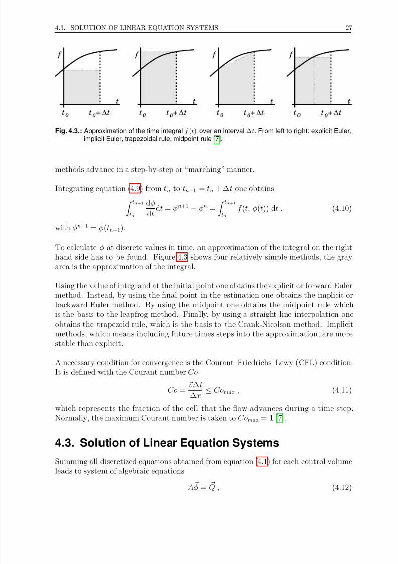
Fig. 4.3.: Approximation of the time integral f (t) over an interval ∆t. From left to right: explicit Euler,implicit Euler, trapezoidal rule, midpoint rule [7].
methods advance in a step-by-step or “marching” manner.
Integrating equation (4.9) from tn to tn+1 = tn + ∆t one obtains tn+1tn
dφ
dtdt = φn+1 − φn =
tn+1tn
f (t, φ(t)) dt , (4.10)
with φn+1 = φ(tn+1).
To calculate φ at discrete values in time, an approximation of the integral on the righthand side has to be found. Figure 4.3 shows four relatively simple methods, the grayarea is the approximation of the integral.
Using the value of integrand at the initial point one obtains the explicit or forward Euler
method. Instead, by using the final point in the estimation one obtains the implicit orbackward Euler method. By using the midpoint one obtains the midpoint rule whichis the basis to the leapfrog method. Finally, by using a straight line interpolation oneobtains the trapezoid rule, which is the basis to the Crank-Nicolson method. Implicitmethods, which means including future times steps into the approximation, are morestable than explicit.
A necessary condition for convergence is the Courant–Friedrichs–Lewy (CFL) condition.It is defined with the Courant number Co
Co = v∆t
∆x ≤Comax , (4.11)
which represents the fraction of the cell that the flow advances during a time step.Normally, the maximum Courant number is taken to Comax = 1 [7].
4.3. Solution of Linear Equation Systems
Summing all discretized equations obtained from equation (4.1) for each control volumeleads to system of algebraic equations
A φ = Q , (4.12)

7/18/2019 120723_Bachelorthesis
http://slidepdf.com/reader/full/120723bachelorthesis 40/73
4.3. SOLUTION OF LINEAR EQUATION SYSTEMS 28
where A is the matrix with the coefficients, φ is the solution vector and Q contains thesource terms.
To solve these equations, direct methods and iterative methods can be used. With directmethods, the solution is determined in one single step. The basic method is the Gaus-
sian elimination, which divides large systems of equations systematically into smallerones. For full matrices, it is one of the fastest and most accurate methods, but usuallymatrices in fluid mechanics are sparse. In addition, the rounding errors can grow rapidlyand therefore the accuracy may be insufficient.
In iterative methods the solution vector φ is corrected until a convergence criterion issatisfied. After n iterations an approximate solution φn is obtained which does notsatisfy the equations (4.12) exactly. Instead, there is a non-zero residual ζ n:
A φn = Q− ζ n (4.13)
To iteratively drive the residual to zero one can write
M φn+1 = N φn + B. (4.14)
Since, at convergence, φn+1 = φn = φ it must be
P A = M −N and B = P Q , (4.15)
where P is a non-singular pre-conditioning matrix. Suitable for iterative methods arethe Jacobi-Iteration, the Gauss-Seidel-Iteration and relaxation methods. There are also
methods which work partly directly and partly iteratively, for example, the block itera-tion, LU (Lower-Upper) iteration and the CG (conjugate gradient) method.

7/18/2019 120723_Bachelorthesis
http://slidepdf.com/reader/full/120723bachelorthesis 41/73
5. Implemented Solver in OpenFOAMand the Cantera Interface
This chapter starts with a short discussion of the used software packages OpenFOAM2.0.1 and Cantera 1.8. Thereafter, the developed interconnection library between Open-FOAM and Cantera is presented. Finally, the implementation of the species and sensibleenthalpy equations as well as the integration of the coupling library into existent solversis showed.
5.1. Software Packages
OpenFOAM Version 2.0.1
OpenFOAMR 1 is an open source object-oriented software package written in C++03.It provides a framework to develop numerical solvers in continuum mechanics. Mainadvantages of the design are the overloaded operators, allowing expressive and versatilesyntax for implementations of complex physical models, the extensive pre- and postpro-cessing tools including complex geometry handling and data in-/output and a wide rangeof implemented discretization schemes and boundary conditions. Additionally, Open-
FOAM provides a good parallelization, a high accuracy and is available free of charge.It has been validated many times and is widely used. Fundamental developments aredone by the OpenFOAM Foundation with contributions from a large community. Thecomplete source code is licensed under the GNU General Public License (GPL) for freeuse and customization [15].
In OpenFOAM the discretization of the solution domain is accomplished by the finitevolume method (FVM) presented before. For the discretization of mathematical equa-tions OpenFOAM provides two basic classes. Implicit discretization is handled by theclass fvm . Using the different overloaded operators, e.g. laplacian or grad, of the class
fvm , adds directly to the solving matrix. Explicit discretization is accomplished by usingthe class fvc . Operators from fvc add a source term to the solving matrix. The userhas the possibility to chose during runtime from a wide range of discretization schemeswhich differ in accuracy, stability and error order (e.g. linear Gauss schemes in second orfourth order for gradients, upwind or cubic divergence schemes, Crank-Nicholson for thetime and many more). OpenFOAM offers many solvers for specific cases like compress-ible, multiphase or reacting flows. Additionally, one can chose during runtime whichturbulence, combustion or thermodynamic model the solver should use [32].
1Open Source Field Operation and Manipulation, registered trademark of OpenCFD Limited

7/18/2019 120723_Bachelorthesis
http://slidepdf.com/reader/full/120723bachelorthesis 42/73
5.2. CONNECTION OF OPENFOAM WITH CANTERA 30
OpenFOAM provides a framework for parallelization via domain decomposition usingdifferent schemes or third-party applications, e.g. Scotch, and the possibility to includedifferent implementations of the Message Passing Interface (MPI), e.g. Open MPI orMPICH2. The solving matrices can be solved using different strategies, e.g. the linearpreconditioned conjugate gradient (PCG) solver for symmetric matrices or the linear
preconditioned biconjugated gradient (PBiCG) solver for asymmetric matrices wherethe pressure-velocity coupling can be solved using a semi-implicit method for pressure-linked equations (SIMPLE) algorithm [7, 32].
Cantera Version 1.8
Cantera from the California Institute of Technology is an object oriented software toolkitfor problems involving chemical kinetics, thermodynamics and transport processes [17].It consists of a kernel written in C++03 which is accessible through a wide range of en-vironments like MATLAB and C++. Cantera provides fast, efficient algorithms and is
highly customizable [33]. The complete source code is licensed under the Berkeley Soft-ware Distribution 3-Clause License (BSD-3) which has been verified as a GPL-compatiblefree software license [34].
In simulation codes for turbulent, reacting flows, like OpenFOAM, Cantera can be usedto evaluate thermodynamic properties, chemical sources or transport coefficients thatappear in the transport equations. Cantera includes highly accurate equations derivedfrom the rigorous kinetic theory of gases presented in chapter 3. The implementationis accomplished following [16]. Due to the mathematically expensive operations on verystiff ordinary differential equation systems and matrices inversion, Cantera makes useof highly specialized software packages like SUNDIALS2, BLAS3 and LAPACK4. To
simulate complex systems, a number of ideal reactors is available [33]. Cantera can readthermophysical, transport and chemical data from data files in the CHEMKIN format,see [35]. Additionally, it is possible to perform sensitivity analysis.
5.2. Connection of OpenFOAM with Cantera
Since the numerical computation of multicomponent transport coefficients is not trivial,see [1, 16], a new implementation into OpenFOAM is not worthwhile. As mentioned inthe section before, Cantera is already capable of calculating accurate multicomponent
transport coefficients needed in the transport equations, see chapter 3. Additionally,Cantera can read transport data files in the CHEMKIN format and the calculation of chemical reaction rates is faster as in OpenFOAM [18], which is an important factorwhile performing time-consuming direct numerical simulations. Both OpenFOAM andCantera use C++ as the main language. Hence, it is possible to include source codefrom Cantera directly into OpenFOAM-classes respectively use Cantera functions inOpenFOAM. Based on the Alternate Chemistry Library for OpenFOAM 1.5 (see [18])
2Suite of nonlinear and differential/algebraic equation Solvers (SUNDIALS)3Basic Linear Algebra Subprograms (BLAS)4Linear algebra package (LAPACK)

7/18/2019 120723_Bachelorthesis
http://slidepdf.com/reader/full/120723bachelorthesis 43/73
5.2. CONNECTION OF OPENFOAM WITH CANTERA 31
the coupling interface between OpenFOAM and Cantera was rewritten to meet the re-quirements of OpenFOAM in Version 2.0.1.
The interface makes use of templates to work with existent solvers through the run-timeselection mechanism. The extensive use of OpenFOAM respectively C++ programming
principles enables easy development of further extensions. Additionally, the couplingoffers access to sensible enthalpies, multicomponent or mixture-averaged transport prop-erties or chemical reaction rates. The input files containing molecular properties andchemical mechanism data are in the classical CHEMKIN compatible format.
5.2.1. Structure of the Interface
As shown in figure 5.1, the new coupling interface consists of several classes. The struc-ture is similar to OpenFOAM’s with numerous classes derived from original source files.
The classes canteraChemistryModel and canteraHsPsiMixtureThermo offer access to celldependent values like the chemical source terms, the enthalpy source term or the trans-port properties. Therefore they are derived from the class canteraMixture , which setsup the physical conditions in Cantera, like temperature, pressure and concentration. Ittherefore contains an object of the class canteraThermo, which calculates cell dependentthermophysical properties through Cantera while making use of an object of the classcanteraGasMixWrapper . The class canteraGasMixWrapper deploys the coupling withoriginal classes from Cantera. It is derived from Cantera’s class IdealGasMix and con-tains an object of Cantera’s class Multitransport .
To guarantee full compatibility to existent reacting flow solvers, the class canteraHsP-siMixtureThermo is derived from the original class hsCombustionThermo and the classcanteraMixture is derived from the original class basicMulticomponentMixture . Conse-quently one can perform downcasts5 in existent solvers to obtain access to functionswhich are newly introduced through classes of the interface, e.g. mass diffusion coeffi-cients.
5.2.2. Integration of the Interface into OpenFOAM
Since the interface offers access to nearly all functions known from the original Open-FOAM classes, one can select during runtime which library calculates physical properties
like sensible enthalpy or viscosity. This is realized with dictionary files in the case di-rectory through OpenFOAM’s runtime-selection mechanism. Note, that in general nochanges on solver’s source code is needed. However, like already mentioned before, Open-FOAM’s original classes do not offer mass diffusion coefficients. Hence, to implementtransport equations like in the section before, the source code of the solver has to bechanged more deeply.
5Type casting is converting an expression of a given type into another type. Downcasting is convertinga bass-class reference or pointer to a derived-class. The opposite process is called upcasting [36, 37].

7/18/2019 120723_Bachelorthesis
http://slidepdf.com/reader/full/120723bachelorthesis 44/73
5.2. CONNECTION OF OPENFOAM WITH CANTERA 32
Fig. 5.1.: Inheritance and dependency diagram for the coupling library. Dotted arrow “contains anobject of”, normal arrow “derived from”.
Figure 5.2 shows the initialization sequence of the coupling library in any solver duringruntime. The order in which the class constructors are called indicates the high level of interconnection between original classes and classes from the interface. It is importantthat the start of the initialization is performed by the original function psiChemistry-ModelNew . This function is already implemented in existent solvers and guaranteesthe connection to OpenFOAM’s runtime selection mechanism. It reads input files andchooses the chemistry class, here the canteraChemistryModel . The function hsCombus-tionThermoNewType chooses the thermo class from input files. Here, the class canteraH-sPsiMixtureThermo is used, which calls the subclass constructors until finally the classcanteraGasMixWrapper deploys the connection to Cantera’s original classes. Listing A.3
in the appendix shows the implementation of the initialization.
5.2.3. Exchange of Data between OpenFOAM and Cantera
To obtain access to derived class properties, like the mass diffusion coefficients, a down-cast shown in listing A.3 in the appendix, has to be performed. Figure 5.3 shows theexchange of data between OpenFOAM and Cantera through the interface canteraFoam-Model . OpenFOAM solves the implemented transport equations for energy, species,velocity and pressure, and passes the thermodynamic data in vectors of dimension num-ber of control volumes N to the interface. The interface then constructs for each singlecontrol volume an independent reactor. For every reactor Cantera calculates cell depen-

7/18/2019 120723_Bachelorthesis
http://slidepdf.com/reader/full/120723bachelorthesis 45/73
5.2. CONNECTION OF OPENFOAM WITH CANTERA 33
Fig. 5.2.: Initialization sequence of the coupling library in a solver during runtime (order: top left first,bottom right last).
dent data like the chemical reaction rates rk or transport properties like µ,λ,Dkj , DT k .Cantera then returns per reactor vectors of dimension number of species K for rk or DT
k ,simple scalars for µ or λ, and matrices of dimension (K × K ) for Dkj . The interfacecollects the values of every cell and constructs vectors or matrices with cell values forevery control volume and returns matrices of dimension (N
×K ) for the reaction rates
or of dimension (N ×K × K ) for the ordinary diffusion coefficients Dkj and vectors of dimension (N ) for µ or κ.

7/18/2019 120723_Bachelorthesis
http://slidepdf.com/reader/full/120723bachelorthesis 46/73
5.3. IMPLEMENTATION OF THE SOLVER 34
Fig. 5.3.: Data exchange between OpenFOAM and Cantera through the interface canteraFoamModel .
5.3. Implementation of the Solver
The new solver is based on the OpenFOAM solver reactingFoam . Transport equationsfor species mass and energy based on equation (3.7) and (3.15) replace the approach
in the original solver discussed in the next subsection. To use functions from Canteralike multicomponent mass diffusion coefficients or reaction rates, the interface presentedabove has to be loaded dynamically during runtime or linked while compiling. Note,that accurate expressions for the continuity equation 3.9 as well as for the momentumequation 3.10 are already implemented in the original solver and therefore not altered.
5.3.1. OpenFOAM’s Approach for Transport Equations
The original transport equations for species and sensible enthalpy are
∂
∂t(ρY k) =
−
∇ ·(ρY kv) +
∇ ·(µ
∇Y k) + rk (5.1)
∂
∂t(ρhs) = − ∇ · (ρhsv) + ∇ · (
λ
c p ∇hs) +
D p
Dt + q reaction (5.2)
One can see, that equation (5.1) is based on the assumption that the ratio of momentumdiffusivity and mass diffusivity is unity. Thus, the dimensionless Schmidt number Scyields
Sc = µ
ρD = 1 → ρD = µ . (5.3)
Therefore, the mass diffusivity D has to be the same for all species and the speciesdiffusion process is entirely controlled by the mixture viscosity, which is calculated from

7/18/2019 120723_Bachelorthesis
http://slidepdf.com/reader/full/120723bachelorthesis 47/73
5.3. IMPLEMENTATION OF THE SOLVER 35
Sutherland’s law. Additionally, cross diffusion process based on pressure and tempera-ture gradients are neglected.
In equation (5.2) a unity Lewis number Le as well as the disregards from above areassumed:
Le = λDc pρ
= 1 → λc p
= ρD (5.4)
It has been shown by [12], that equations (5.1) and (5.2) yield large errors while simu-lating chemically reacting flows.
5.3.2. Implementation of Species Mass Equations
In nearly isobar combustion the flux caused by the pressure gradient in equation (3.20)can be neglected. External forces occur for example in the diffusion of electrically chargedparticles and will be neglected, too. With these simplifications and the relation
∇X j = M
M j ∇Y j − Y j
M
M j
N i=1
M
M i ∇Y i , (5.5)
equation (3.20) can be rearranged to
jk = ρM kM
N j=1
Dkj ∇Y j − ρM kM
N j=1
DkjY jN i=1
M
M i ∇Y i −DT k
1
T ∇T , (5.6)
to obtain the mass diffusive flux in terms of mass fractions.
For numerical stability, including a discretized second derivation or diffusion term intothe solution matrix is essential [7]. A direct implementation of the mass diffusive fluxequation (5.6) is therefore not worthwhile, because of the missing diffusion terms whichcan be discretized implicit by OpenFOAM’s class fvm . Through the use of the, insection 3.3 already mentioned, characteristics of the ordinary diffusion coefficient matrix,equation (5.6) is rearranged to
jk =N j=k
ρM kM
Dkj ∇Y j −N j=k
N i=k
M kM i
ρDkjY j ∇Y i −H j=k
ρDkjY j ∇Y k −DT k1
T ∇T , (5.7)
so that the third term on the right hand side can be discretized implicit by OpenFOAM.
Finally, by inserting the expression for the mass flux above into equation (3.7) thetransport equation for species k reads
∂
∂t(ρY k) + ∇ · (ρY kv)−
N j=k
∇ · (ρDkjY j ∇Y k) =
−N j=k
∇ ·
ρM kM
Dkj ∇Y j
+
N j=k
N i=k
∇ ·
M kM i
ρDkjY j ∇Y i
+ ∇ ·
DT k
1
T ∇T
+ rk ,
(5.8)

7/18/2019 120723_Bachelorthesis
http://slidepdf.com/reader/full/120723bachelorthesis 48/73
5.3. IMPLEMENTATION OF THE SOLVER 36
in which all terms discretized implicit by OpenFOAM’s class fvm stand on the left handside and all terms included and calculated as explicit source terms by OpenFOAM’s class fvc stand on the right hand side. Listing A.1 in the appendix shows the implementationof equation (5.8) in OpenFOAM.
5.3.3. Implementation of Sensible Enthalpy Equation
As mentioned above a diffusive flux term has to be included into the solution matrix.Therefore, it is necessary to express Fourier’s Law in terms of sensible enthalpy. Startingwith an expression of the enthalpy gradient for a multicomponent gas mixture givenby [21],
∇h = c p ∇T +N k=1
hk ∇Y k , (5.9)
one can, by express the specific enthalpy with the sum of sensible and chemical enthalpy(3.13), modify Fourier’s law to
λ ∇T = λ
c p ∇h−
N k=1
λ
c phk ∇Y k
= λ
c p ∇hs +
N k=1
λ
cphc,k ∇Y k −
N k=1
λ
c phc,k ∇Y k −
N k=1
λ
c phs,k ∇Y k
= λ
c p ∇hs −
N k=1
λ
c phs,k ∇Y k . (5.10)
Now, the first term on the right hand side can be discretized implicit by OpenFOAM.
The diffusive species flux from equation (3.31) in terms of sensible Enthalpy gives
N k=1
jkhk =N k=1
jk(hc,k + hs,k) . (5.11)
Combining equations (3.15), (3.31), (5.10), (5.11) and neglecting viscous dissipation
τ : ∇v and the Soret effect one obtains
∂
∂t(ρhs) + ∇ · (ρhsv)− ∇ ·
λ
c p ∇hs
=
D p
Dt −
N k=1
∇ ·
λ
c phs,k ∇Y k
−
N k=1
∇ · (hs,k jk)−N k=1
hc,k rk ,(5.12)
in which all terms discretized implicitly by OpenFOAM’s class fvm stand on the left handside and all terms included and calculated as explicit source terms by OpenFOAM’sclass fvc stand on the right hand side. The diffusive species flux jk is calculated byinterpolation from the species equation noted in listing A.1 as “J[k]”. Listing A.2 in theappendix shows the implementation of equation 5.12 in OpenFOAM.

7/18/2019 120723_Bachelorthesis
http://slidepdf.com/reader/full/120723bachelorthesis 49/73
6. Validation of the SolverIn this chapter, the implemented solver introduced in chapter 5 is validated with focuson the transport properties and reaction rates. The reference solution is obtained fromCHEMKIN/PREMIX with equal physical conditions. In addition, the effect of the gridresolution onto the solution and the chemical time scales are investigated.
6.1. Case Description
Figure 6.1 shows the physical domain of the considered case. Here, the fresh gas mixtureflows from the left into the domain. Due to thermal conduction, the mixture is preheated(dark blue) until it ignites (light blue). In the following, the outburn proceeds (red zone)and the adiabatic flame temperature is reached.
λ Y CH 4,in Y O2,in Y N 2,in T in [K] p [bar] vx,in [m/s]
1.0 0.055 0.2202 0.7248 300 1.0 0.4
Tab. 6.1.: Physical conditions of the simulation with OpenFOAM.
The mixture is stoichiometric with λ = 1 and the mass fractions at the inlet are Y O2,in =0.2202, Y CH 4,in = 0.055 and Y N 2,in = 0.7248. The fluid’s temperature at the inlet isT in = 300 K with an inflow velocity vx,in = 0.4 m/s. The pressure in the whole domainas well as outside is constantly p = 1 bar. The physical conditions (shown in table 6.1)are chosen to be the same as in the reference calculation.

7/18/2019 120723_Bachelorthesis
http://slidepdf.com/reader/full/120723bachelorthesis 50/73
6.2. NUMERICAL CONDITIONS 38
Fig. 6.1.: Physical domain of the laminar, premixed flame.
6.2. Numerical conditions
Table 6.2 shows the numerical setup of the various simulations performed with the newsolver in OpenFOAM. The different grids consist of 600 and 3000 equidistant rectangularcells built with the blockMesh tool from OpenFOAM. The grid resolutions are ∆x =5 × 10⁻⁵m and ∆x = 1 × 10⁻⁵m for each cell. The time steps are set to ∆t = 5 ×10⁻⁷s on the coarse grid and ∆t = 1 × 10⁻⁷s on the fine mesh. For all simulation,including the reference calculation, the mechanism by [38], which contains 17 species
and 58 reactions (see Appendix B), is used to calculate the chemical kinetics. Forthermodynamic and molecular properties the same input files are used in OpenFOAMand CHEMKIN/PREMIX.
Domain [m] Cells ∆t [s] ∆x [m]
Coarse 0.03 600 5× 10⁻⁷ 5× 10⁻⁵
Fine 0.03 3000 1× 10⁻⁷ 1× 10⁻⁵
Tab. 6.2.: Numerical setups.
Figure 6.2 shows the numerical domain. At the inlet, fixed values are chosen as bound-ary condition for all physical properties. The boundary conditions at the outlet differbecause of different requirements. For mass fraction and temperature a simple zero gra-dient boundary condition is adequate. To control possible backflow at the outlet a mixedboundary condition, the inletOutlet condition, is needed for the velocity. It switches theboundary condition between a fixed value and zero gradient depending on direction of the velocity. Since the numerical domain is just a clipping of the infinity large physicaldomain, the front, back, top and bottom sides are defined empty. Additionally, the nu-merical domain is only divided into cells, marked by the dashed lines, in the x-direction.Therefore, only a solution in this direction is approached leading to a one dimensionalcase.

7/18/2019 120723_Bachelorthesis
http://slidepdf.com/reader/full/120723bachelorthesis 51/73
6.2. NUMERICAL CONDITIONS 39
Fig. 6.2.: Numerical domain of the laminar, premixed flame.
In the calculations the implicit Euler method is used to discretize the time integral.Like mentioned in chapter 4 the implicit Euler method is of order O(1)t. The spatialdiscretization is accomplished via Gaussian integration and using linear interpolatingschemes of orderO(2)x. The discretization schemes used in OpenFOAM for the differentterms in the transport equations are listed in table 6.3.
Mathematical Term Expression in OpenFOAM Discretization Order
∂φ/∂t ddt Euler implicit O
(1)t
∇(φ) grad Gauss linear O(2)x
∇ · φ div Gauss linear/limitedLinear 1 O(2)x
∇ · (∇φ) laplacian Gauss linear corrected O(2)x
− interpolation linear O(2)x
Tab. 6.3.: In OpenFOAM used discretization schemes for the mathematical terms.
To obtain similar conditions like in CHEMKIN/PREMIX, no transport equation for ve-locity and pressure is solved. The remaining transport equations are solved using differ-ent iterative solver and preconditioners, namely for density the Preconditioned conjugate
gradient (PCG) solver with Diagonal incomplete-Cholesky (DIC) preconditioning andfor sensible enthalpy and species mass fractions the Preconditioned biconjugate gradient(PBiCG) solver with Diagonal incomplete-LU (DILU) preconditioning.
For the initialization of the simulation a homogeneous flow field with conditions like atthe inlet is shortly ignited. Therefore, an spatial limited source term is included in thetransport equation of enthalpy with an ignition strength of 5 × 10⁹ J/m3·s for 0.0002 s.In the ignited cells two flame fronts develop. The downstream traveling flame frontleaves the domain and is not of further interest.

7/18/2019 120723_Bachelorthesis
http://slidepdf.com/reader/full/120723bachelorthesis 52/73
6.3. COMPARISON WITH CHEMKIN/PREMIX 40
6.3. Comparison with CHEMKIN/PREMIX
To validate the OpenFOAM solver a simulation with 3000 cells is performed. The focusof the validation are the newly implemented equations for species and sensible enthalpyas well as the transport coefficients and reaction rates obtained from Cantera. The
calculations are compared to results obtained from CHEMKIN/PREMIX with similarconditions. CHEMKIN/PREMIX is a highly specialized computer code for premixedlaminar flames in 1D [20]. The code presumes isobar conditions and a steady state flame.To get similar conditions in OpenFOAMR no pressure correction is performed and thevelocity field is calculated from
m
A = ρ0v0 = ρv = const. → v =
ρ0v0
ρ and ρ =
p
T Rs. (6.1)
in which Rs = R/M is the specific gas constant of the mixture. For this reason, thepressure is forced to remain constant at all times in the complete domain. Furthermore,in CHEMKIN/PREMIX the inlet mass flux m is changed during the simulation in sucha way to hold the flame front steady. Due to missing moving mesh features implementedinto the new solver it is therefore not possible to completely prevent a motion of theflame front. CHEMKIN/PREMIX is capable of dynamic mesh refinement and appliesfor the current case a total number of only 185 grid points with the minimal distance of ∆xmin ≈ 3× 10⁻⁶m.
6.3.1. Temperature and Species Mass Fractions
In figure 6.3 the temperature profile from 3000 Cells (solid) is compared to the refer-ence calculation (circles). The solutions are nearly the same, a part from two notable
disagreements at the beginning and the end of the inner reaction zone with maximumvariations of about 17 K. One can see, that the grid used by CHEMKIN/PREMIX atthe beginning of the reaction zone is too low against the fine mesh from OpenFOAM.Additionally, the discretization scheme used by CHEMKIN/PREMIX is the backward-difference scheme. It is of order one and introduces, similar to the upwind interpolation(UDS) mentioned before, artificial diffusion. Therefore, CHEMKIN/PREMIX spreadsout the solution on a coarse mesh [7, 20] and can not resolve the large gradient as accu-rately as OpenFOAM.
Case Y COmax Y CH 3max Y OH max Y H 2max sL [m/s]
CHEMKIN/PREMIX 0.051967 0.00277 0.00510 0.00163 0.373
OpenFOAM 0.05240 0.00274 0.00497 0.00163 0.376
Deviationa 0.83 % 1.08 % 2.54 % 0.00 % 0.8 %
a Deviation based on CHEMKIN/PREMIX calculations
Tab. 6.4.: Comparison of distinctive results obtained with OpenFOAM and CHEMKIN/PREMIX.
In figure 6.3 the species mass fractions Y CH 4, Y O2 , Y CO2, Y CO and Y H 2O (solid) are com-
pared to the reference calculation (circles). As one can see, the solution obtained from

7/18/2019 120723_Bachelorthesis
http://slidepdf.com/reader/full/120723bachelorthesis 53/73
6.3. COMPARISON WITH CHEMKIN/PREMIX 41
OpenFOAM is very similar to the reference solution. The profiles of intermediate speciesmass fractions Y OH , Y O, Y H 2, Y CH 3 and Y CH 2O as well as the minimal species mass frac-tions Y CH 2 , Y H , Y H 2O2, Y HCO and Y HO2 confirm that conclusion, although there are tinydiscrepancies (see table 6.4) between the reference calculation and OpenFOAM whichhave a maximum variation at Y OH of about 1.3
×10−4. Again, the different grid reso-
lution between OpenFOAM and CHEMKIN/PREMIX in these regions may be the rea-son. By using equation (2.4) the laminar burning velocity calculates to sL = 0.376 m/s.As one can see in table 6.4 this is very similar to the value obtained from CHEMK-IN/PREMIX. Additionally, a comparison with experimental results, e.g. [39], confirmsa very good agreement of OpenFOAM’s value, too.
1 1.05 1.1 1.15 1.2
500
1000
1500
2000
Axial distance x [cm]
T e m p e r a t u r e T
[ K ]
OpenFOAM
CHEMKIN
1 1.05 1.1 1.15 1.2
0
0.1
0.2
CH 4
O2
CO2
H 2O
CO
Axial distance x [cm]
M a s s f r a c t i o n Y
[ - ]
1 1.05 1.1 1.15 1.2
0
2
4
·10−3
OH
O
H 2
CH 3
CH 2O
Axial distance x [cm]
M a s s f r a c t i o n Y
[ - ]
1 1.05 1.1 1.15 1.2
0
1
2
3
·10−4
CH 2
H
H 2O2
HCO
HO2
Axial distance x [cm]
M a s s f r a c t i o n Y
[ - ]
Fig. 6.3.: Temperature and species mass fraction profiles obtained from OpenFOAM (lines) and fromCHEMKIN/PREMIX (circles).

7/18/2019 120723_Bachelorthesis
http://slidepdf.com/reader/full/120723bachelorthesis 54/73
6.4. INFLUENCE OF THE GRID RESOLUTION 42
6.4. Influence of the Grid Resolution
The calculation time in a numerical simulation highly scales with the number of cells [7].Therefore, knowledge about the influence of the grid resolution and the time step ontothe solution is essential. In this section the validated grid from the previous section with
3000 cells is compared to the coarse grid with 600 cells. The CFL number was kept thesame leading to time steps up to ∆t = 5× 10⁻⁷ s.
In figure 6.4 the temperature profile obtained with 600 Cells (dashed) is compared to theone obtained with 3000 Cells (cross). The two noticeable disagreements at the beginningand the end of the inner reaction zone show maximum variations of about 15 K.
The heat release calculated from equation 3.16 is shown at the bottom of figure 6.4. Onecan see, that the reaction zone is slightly displaced and thicker in the solution obtainedwith the coarse grid compared to the one obtained with the finer grid. This is consistent
with the mass fraction profiles mentioned further down. Moreover, one can identify, thatmost of the heat is released at higher temperatures. Upstream from the flame front, nochemical reactions occur and the temperature rises due to thermal conduction.
Case Y COmax Y CH 3max Y OH max Y H 2max sL [m/s]
600 Cells 0.05080 0.00248 0.00497 0.00162 0.385
3000 Cells 0.05240 0.00274 0.00497 0.00163 0.376
Deviationa 3.14 % 10.0 % 0.0 % 0.61 % 2.33 %
a Deviation based on 600 Cells calculations
Tab. 6.5.: Comparison of distinctive results obtained with 600 Cells and 3000 Cells.
Figure 6.4 shows the major species mass fractions Y CH 4, Y O2, Y CO2, Y CO and Y H 2O for 600
Cells (dashed) compared to 3000 Cells (line). One can see, that the solution obtainedfrom the coarser grid is very similar to the one obtained with the finer grid. Theprofiles of the minor species mass fractions Y OH , Y O, Y H 2, Y CH 3 and Y CH 2O as well as theminimal species mass fractions Y CH 2, Y H , Y H 2O2 , Y HCO and Y HO2 in figure 6.4 confirmthis conclusion. From the differences between the mass fractions profiles of 600 Cellsand 3000 Cells one can see, that the peaks of the intermediate species differ only slightlyin magnitude and spatial position. The laminar burning velocity sL is nearly the samefor all grids.

7/18/2019 120723_Bachelorthesis
http://slidepdf.com/reader/full/120723bachelorthesis 55/73
6.4. INFLUENCE OF THE GRID RESOLUTION 43
1 1.05 1.1 1.15 1.2
500
1000
1500
2000
Axial distance x [cm]
T e m p e r a t u r e T
[ K ]
Coarse
Fine
1 1.05 1.1 1.15 1.2
0
0.1
0.2
CH 4
O2
CO2
H 2O
CO
Axial distance x [cm]
M a s s f r a c t i o n Y
[ - ]
1 1.05 1.1 1.15 1.2
0
1
2
3
4
5
·10−
OH
O
H 2
CH 3
CH 2O
Axial distance x [cm]
M a s s f r a c t i o n Y
[ - ]
1 1.05 1.1 1.15 1.2
0
1
2
3
·10−
CH 2
H
H 2O2
HCO
HO2
Axial distance x [cm]
M a s s f r a c t i o n Y
[ - ]
1 1.05 1.1 1.15 1.2
0
1
2
3
4
·10
Axial distance x [cm]
H e a t r e l e a s e r a t e ˙ q
[ J / m
3 ·
s ]
Fig. 6.4.: Profiles obtained from OpenFOAM with 600 Cells (dashed line) and 3000 Cells (line).

7/18/2019 120723_Bachelorthesis
http://slidepdf.com/reader/full/120723bachelorthesis 56/73
6.5. SPECIES PRODUCTION RATES 44
6.5. Species Production Rates
In figure 6.5 the computed reaction rates for the species are shown. By comparing thereaction rates with the mass fraction profiles from the section before, one can see, thatspecies with high diffusion coefficients (e.g. H radicals) diffuse upstream against the flow
into the preheat region. Here, H O2 begins to form which is later, at higher temperatures,transformed into OH radicals. The OH radicals become relatively abundant versus theO or H radicals to latter stages of the reaction zone. Throughout the reaction zone, C Omolecules build up until they are rapidly consumed by the abundant OH radicals. Thisis responsible for the major heat release of the combustion process and also marks theend of the reaction zone.
1 1.05 1.1 1.15 1.2
−400
−200
0
200
CH 4
O2
H 2O
CO2
CO
Axial distance x [cm]
R e a c t i o n r a t e r
[ k g / m
3 ·
s ]
1 1.05 1.1 1.15 1.2
−40
−20
0
20
40
CH 3
CH 2O
O
OH
H 2
Axial distance x [cm]
R e a c t i o n r a t e r
[ k g / m
3 ·
s ]
1 1.05 1.1 1.15 1.2
−5
0
5
HCO
HO2
H
CH 2
H 2O2
Axial distance x [cm]
R e a c t i o n r a t e r
[ k g / m
3 ·
s ]
Fig. 6.5.: Reaction rates obtained from OpenFOAM.
6.6. Computation of Chemical Time Scales
To determine the necessary time step for the numerical simulation of the turbulentpremixed flame the chemical time scales were calculated from equation (3.39). Figure

7/18/2019 120723_Bachelorthesis
http://slidepdf.com/reader/full/120723bachelorthesis 57/73
6.6. COMPUTATION OF CHEMICAL TIME SCALES 45
6.6 shows the time scales for T , O2 and OH against the temperature.
300 600 900 1200 1500 1800 210010−5
10−4
10−3
10−2
10−1
100
T
O2
OH
Temperature T [K]
C h e m i c a l t i m e s c a l e τ
[ s ]
Fig. 6.6.: Calculated chemical time scales τ for T , O2 and OH .
One can see, that in an region, which corresponds to the main reaction zone, the timescales are almost constant. For intermediate species the time scales show characteristicpeaks which correspond to formation and oxidation reactions. The minimum of thecalculated time scales determines the chemical time scale of the simulation. Here, the
time scale ranges between 10−5
s and 10−4
s. The time scale of temperature, which isthe most important for combustion modeling, is 2 × 10⁻⁴ s in this case.

7/18/2019 120723_Bachelorthesis
http://slidepdf.com/reader/full/120723bachelorthesis 58/73
7. Direct Numerical Simulation of aTurbulent Premixed Flame in 3D
In this chapter, the simulation of a turbulent premixed flame in 3D is presented. Themain purpose is to show that a direct numerical simulation of turbulent reacting flowusing the validated solver is in principle possible. Therefore, the results are only brieflydiscussed with main focus on the flame topology. In addition, since the simulations arecarried out on a Cray XE6 supercomputer [40], the parallel performance of the solver inconjunction with the supercomputer is investigated.
7.1. Numerical Setup
Based on the results from the last chapter, the physical and numerical conditions arechosen, see table 7.1. It has been shown before, that a numerical grid with ∆x = ∆y =∆z = 5 × 10⁻⁵m and a time step ∆t = 5 × 10⁻⁷s is a good compromise between thedesired accuracy and calculation time. This conclusion is later approved by the cal-culated Kolmogorov scales. Figure 7.1 shows the computational domain for the threedimensional case. The dimension is (1.5×0.75×0.75) cm3, which is thus half the lengthto the one dimensional case, with 300
×150
×150 = 6.75
×106 equidistant cells of size
∆x = ∆y = ∆z = 5 × 10⁻⁵m. The physical conditions listed in table 7.1 are similarto the one dimensional case in chapter 6 except for the inlet velocity field which hasthe mean value vin = 4.0 m/s and fluctuates with vin = 2 m/s. The Reynolds numberbased on integral dimensions at the inlet is Re = 2000. The main differences, besidesthe turbulence, are the three dimensional resolution of the shorter physical domain andthe needed solution of three additional transport equations for velocity and one equationfor pressure-correction. For chemical kinetics and thermodynamic properties as well asmolecular quantities the same input files are used as before. The total simulation timeis approximately 5 ms, which leads to a wall-clock time of approximately 48 hours onthe Cray XE6 with 2048 CPUs.
λ Y CH 4,in Y O2,in Y N 2,in T in [K] p [bar] vin [m/s] vin [m/s] Re
1.0 0.055 0.2202 0.7248 300 1.0 4.0 2.0 2000
Domain [m] Cells ∆t [s] ∆x [m] Discret. Order
(0.015× 0.0075× 0.0075) 6.75× 10⁶ 5× 10⁻⁷s 5× 10⁻⁵ O(2)x O(1)t
Tab. 7.1.: Physical and numerical conditions of the turbulent, premixed flame in 3D.

7/18/2019 120723_Bachelorthesis
http://slidepdf.com/reader/full/120723bachelorthesis 59/73
7.1. NUMERICAL SETUP 47
Since the flow is three dimensional, solutions in directions outside the domain (in addi-tion to the in- and outlet) are needed. To ensure, that no mass is lost, the front, back,top and bottom faces of the domain are defined as symmetry planes. The boundaryconditions at the in- and outlet for temperature T and species mass fractions Y i arethe same as for the one dimensional case. To avoid reflections of pressure waves at
the in- and outlet, non-reflective boundary conditions (NRBC) are used for pressure.To generate a turbulent flow at the inlet a turbulent inflow generator by [ 41] is usedfor the velocity field. The boundary condition is based on digital filtering of randomdata to provide temporally and spatially correlated velocities. The mean flow velocityis vin = 4.0 m/s with a turbulence level of 50 %. The turbulent length scale lT and theturbulent time scale τ T are set to lT = 1 mm and τ T = 0.5 ms.
Fig. 7.1.: Numerical domain of the turbulent, premixed flame.

7/18/2019 120723_Bachelorthesis
http://slidepdf.com/reader/full/120723bachelorthesis 60/73
7.2. INITIAL CONDITIONS 48
7.2. Initial conditions
The initial conditions have been produced by a DNS on the same computational grid,however, without chemical reactions. Then, the flat flame front with suitable tempera-ture and mass fraction fields from the one dimensional case has been superimposed into
the flow. Figure 7.2 shows the initial velocity and the temperature fields right beforethe simulation starts. One can see, that the flame front (marked with red colors) is stillplanar since the passed time is short.
Fig. 7.2.: Initial velocity and temperature fields of the premixed turbulent flame.
Figure 7.3 shows the Kolmogorov scales. They are calculated from the produced initialconditions by using equations (2.6). One can see, that the Kolmogorov length scale lLvaries between 2× 10⁻⁵ m and 2.5× 10⁻⁴ m. Since the small values occur mostly nearthe inlet the used grid spacing can be expected to resolve the smallest eddies near theflame front sufficiently. The Kolmogorov time scale τ K varies between 2 × 10⁻⁵ s and
2.83× 10⁻³
s. Since τ K is relatively great, the used time step is limited by the Courantnumber due to numerical stability reasons.
Fig. 7.3.: From the initial conditions calculated Kolmogorov scales.

7/18/2019 120723_Bachelorthesis
http://slidepdf.com/reader/full/120723bachelorthesis 61/73
7.3. TOPOLOGICAL RESULTS 49
7.3. Topological Results
The main purpose is to show, that a direct numerical simulation of turbulent reactingflow using the validated solver is possible. Therefore, the results are given only brieflywith main focus on the flame topology. Figure 7.4 shows an isosurface of the heat
release rate, which can be taken as the position of the flame front. The heat releaserate is calculated by using equation (3.16). A corrugated surface, which is caused bythe turbulent flow shown in the back can be identified. On the bottom of figure 7.4 theeddy dissipation rate is shown. The eddy dissipation rate is very high at the flame frontand near zero downstream, since no eddies are present anymore.
Fig. 7.4.: Isosurface of Y CH 4 . Bottom with eddy dissipation rate and backside with vorticity.
The ratio of mean flame surface and turbulent flame surface calculates to AT
A = 2.33.
Additionally, by using equation 2.10 the turbulent burning velocity calculates to sT =
0.704 m/s, which is less than two times the laminar burning velocity calculated for thelaminar flame in the chapter before. The difference in the laminar flame velocities iscaused by the curved and stretched turbulent flame.
Figure 7.5 shows contour plots of the temperature and velocity field. The flame frontis marked by iso-contours of the heat release rate. The structure of the turbulence isvisible at the inlet and the flow is accelerated by passing the flame front. The temper-ature increases over the flame front from 300 K up to 2200 K. The velocity gradientsin the burnt mixture are clearly smaller caused by high viscosity. A distinct featureof the flame topology is the presence of an instantaneous wrinkled flame front. In ar-eas in which the flame front wrinkles with a convex geometry into the burnt gas, the

7/18/2019 120723_Bachelorthesis
http://slidepdf.com/reader/full/120723bachelorthesis 62/73
7.3. TOPOLOGICAL RESULTS 50
Fig. 7.5.: Two dimensional slices of the temperature field and the vorticity field with heat release rateof the turbulent premixed flame.
heat release is higher. Additionally, due to the turbulent flow, the flame front varies inthickness. In this case, small eddies penetrate the flame front and enhance the diffusionprocess, leading to a thickened flame front. In areas where the cold flow is slow the flamefront even propagates into the unburnt gas. It is evident that the vorticity is greatlydamped in the burned gas side because the gas viscosity increases with temperature.
Additionally, in figure 7.6 the mass fractions of CH 4, O2, H 2 and OH as well as thecorresponding reaction rates are shown. One can see, how the reaction zone varies inthickness and the strain of the flame front influences the reaction rates.

7/18/2019 120723_Bachelorthesis
http://slidepdf.com/reader/full/120723bachelorthesis 63/73
7.3. TOPOLOGICAL RESULTS 51
Fig. 7.6.: Different mass fractions and reaction rates.

7/18/2019 120723_Bachelorthesis
http://slidepdf.com/reader/full/120723bachelorthesis 64/73
7.4. PARALLEL PERFORMANCE OF THE CRAY XE6 (HERMIT) 52
7.4. Parallel Performance of the Cray XE6 (HERMIT)
To perform direct numerical simulations of chemically reacting flows, at least three ve-locity equations, one mass equation, one enthalpy equation and K − 1 species equationshave to be solved iteratively. The number even increases if pressure-velocity coupling
schemes are used [7]. In addition, calculations for the chemical reaction rates or trans-port properties have to be performed at least once per time step and cell. In particular,the calculation time of multicomponent mass diffusion coefficients, shown in section 3.3,requires the inversion of a K ×K matrix [16]. Further more, if turbulent flow is consid-ered, it can be shown, that the number of grid points in each direction must be at leastl/lK [7].
Due to the small time steps and the high grid resolution, direct numerical simulations of chemically reacting flows have to be performed in parallel on high performance comput-ing clusters. Since the architecture of each cluster is very unique and an efficient usage
of existing resources is essential one has to know about the speed-up particularly of highperformance clusters.
The numerical simulation of the turbulent premixed flame in 3D presented before wasperformed on the Cray XE6 (HERMIT) operated by the High Performance ComputingCenter Stuttgart (HLRS). It is a massively parallel supercomputer with 3552 computenodes. Each compute node has two sockets with each 16 AMD Interlagos processors.Each XE6 node has either 32 or 64 GB of DDR3 SDRAM memory. The node-nodeinterconnection is based on CRAY Gemini. The XE6 is operated with the Cray LinuxEnvironment in version 3, including SUSE Linux Enterprise Server and Cray’s ComputeNode Linux [40, 42].
For the current investigation, several calculations have been carried out to obtain in-formation about parallel efficiency and scalability. The new OpenFOAM solver (seechapter 5) has been used and the conditions for all calculations where the same exceptfor the number of cores. The mesh consists of about 2× 10⁶ cells.

7/18/2019 120723_Bachelorthesis
http://slidepdf.com/reader/full/120723bachelorthesis 65/73
7.4. PARALLEL PERFORMANCE OF THE CRAY XE6 (HERMIT) 53
Figure 7.7 shows the intranode scale-up (left) and internode scale-up (right) calculatedwith S n = ts/tn [7]. Here ts is the execution time with the reference processor numberand tn is the execution time using n processors. The reference processor number for theintranode scale-up is 1 CPU and for the internode scale-up equal the number of CPUsper node (32 CPUs). One can see, that the intranode speedup is far from the linear
speed up marked as a solid line. Thus, it is not worthwhile using the Cray XE6 withonly a few CPUs on one node. On the contrary, the internode performance scales verywell up to 2048 processors. Between 64 processors and 1024 processors the scale-upis even superlinear1[7]. The scale-up indicates a very good scalability of Cray XE6 inconjunction with the solver even for 6.75 × 10⁶ Cells. Therefore, in the DNS of theturbulent flame in the section before 2048 CPUs have been used.
20
21
22
23
24
25
= 32
20
21
22
23
2
4
25
ideal
No. of CPUs
I n t r a n o d e
s c a l e - u p
25
27
29
211
= 2048
20
22
24
26
ideal
No. of CPUs
I n t e r n o d e
s c a l e - u p
Fig. 7.7.: Scale-up on Cray XE6 with a grid of 2 × 10⁶ cells.
1Superlinear is a speedup of more than p if p processors are used. It occurs rarely in parallel computing.[43] showed with a simple example how a superlinear speedup is achieved.

7/18/2019 120723_Bachelorthesis
http://slidepdf.com/reader/full/120723bachelorthesis 66/73
8. Summary and PerspectiveA solver for direct numerical simulations of chemically reacting flows has been imple-mented and validated for the free CFD framework OpenFOAM 2.0.1. The solver takesdetailed multicomponent diffusive fluxes into account. The molecular transport coeffi-cients as well as the chemical kinetics and thermodynamic quantities were obtained viaa coupling interface from Cantera 1.8. The solver as well as the coupling library weresuccessfully compiled with an MPI implementation on the Cray XE6 for the parallelizedcomputation of DNS of turbulent reacting flows.
To validate the solver, numerical calculations of a laminar premixed flat flame have beencarried out. The results were subsequently compared to reference data obtained fromthe CHEMKIN package. The agreement with respect to the computed flame profiles forT and Y was very good. The calculated flame speed showed reasonable results with ex-perimental data. Additional calculations were performed on a coarse grid to investigatethe influence of the gird resolution on the computed flame structure. The results wereshown to depend very little on whether the coarse or fine mesh had been used. Subse-quently, direct numerical simulation of a turbulent premixed flame in three dimensionshave been performed on the Cray XE6 supercomputer with 2048 CPUs. The interactionbetween turbulence and the flame front has been identified. Thereby, the capability of
the solver for complex 3D turbulent flows with chemical reactions as well as the verygood scale-up on the Cray XE6 was shown.
For future work, the validated DNS solver will be used for further investigations of theinterplay between turbulence and chemical reactions as well as characteristic values likestrain rate, the curvature or the turbulent burning velocity. The influence of selectivediffusion mechanisms (like e.g. the Soret effect) on the numerical solution of turbulentpremixed flames can be studied. Furthermore, essential statistical information, which isneeded to develop and validate models used in future RANS and LES simulation, canbe provided by the DNS solver.
Thanks to the usage of C++ programming principles it is possible to extend the solver byincluding new numerical or computational utilities in order to study additional physicalphenomena. The investigation of details like the radiative heat transport or the Dufoureffect can further enrich such a study. In order to reduce the CPU time in numericalsimulations a mixture average approach for the diffusive fluxes can be included as well asan adaptive mesh refinement based on characteristic gradients. Equations for the stretchrate or flame velocity and models for soot or N Ox formation can also be incorporatedand validated for further examination of turbulent premixed flames.

7/18/2019 120723_Bachelorthesis
http://slidepdf.com/reader/full/120723bachelorthesis 67/73
A. Code Fragments for OpenFOAM inC++3
The following listings show code fragments from the implemented OpenFOAM solver.Listing A.1 shows the implementation of the transport equation (5.8) for species andlisting A.2 shows the implementation of the transport equation (5.12) for sensible en-thalpy. In addition, listing A.3 shows the implementation of the initialization of thecoupling interface and a downcast to obtain access to derived class functions. Note, thatfor the sake of clarity, the codes are simplified and will not compile without modifications.
1 f v Sc a l a r M a t r i x YEqn2 (3 fvm : : ddt( rho , Y[ k ] )4 + mvConvection−>fvmDiv( phi , Y[ k ] )5 ==6 che mis try .RR(k)7 ) ;8
9 f o r A l l (Y, j )10 11 i f ( j !=k)12 13 f o r A l l (Y, i )14 15 i f ( i ! = k )16 17 YEqn −= fv c : : la pl ac ia n (W[ k ]/W[ i ]∗ rho∗ comp ositi on .D(k , j ) ∗Y[ j ] ,
Y [ i ] , " l a pl a c i a n ( D, Y [ k ] ) " ) ;18 J [ k ] −= fv c : : in te rp ol at e (W[ k ]/W[ i ]∗ rho∗ compo sitio n .D(k , j ) ∗Y[ j ]) ∗
( fvc : : in te rp ol at e ( fvc : : grad (Y[ i ]) ) & mesh. Sf () ) ;19 20 21
22
YEqn −= f vm : : l a pl a c i a n ( r ho∗ comp ositi on .D(k , j ) ∗Y [ j ] , Y [ k ] ," la pl ac ia n (D, Yi) " ) ;23 J [ k ] −= f v c : : i n t e r p o l a t e ( r h o∗ compo sitio n .D(k , j ) ∗Y[ j ]) ∗
( fvc : : in te rp ol at e ( fvc : : grad (Y[ k ] ) ) & mesh. Sf () ) ;24
25 YEqn += f vc : : la pl ac ia n ( rho∗W [ k ]∗ UnitMole ∗Wm∗ comp ositi on .D(k , j ) , Y[ j ] ," lap la ci an (D,Y[ k ] ) " ) ;
26 J [ k ] += f v c : : i n t e r p o l a t e ( r h o∗W [ k ]∗UnitMole ∗Wm∗ comp ositi on .D(k , j ) ) ∗( fvc : : in te rp ol at e ( fvc : : grad (Y[ j ]) ) & mesh. Sf () ) ;
27 28 29
30 YEqn
−= f v c : : l a p l a c i a n ( c o mpo s i t i o n .DT( k ) /T , T , " l a pl a c i a n ( D, Y [ k ] ) " ) ;

7/18/2019 120723_Bachelorthesis
http://slidepdf.com/reader/full/120723bachelorthesis 68/73
56
31 J [ k ] −= f v c : : i nt e r po l a t e ( c o mpo s i t i o n . DT( k ) /T ) ∗( fvc : : i nt er po la te ( fv c : : grad (T) ) & mesh. Sf () ) ;
32
33 YEqn. r el ax () ;34 so lv e (YEqn, mesh. so lv er ( "Y[k ] " ) ) ;
Listing A.1: Implementation of the species equation 5.8 in OpenFOAM.
1 f v S c a l a r M a t r i x h sEq n2 (3 fvm : : ddt( rho , hs )4 + mvConvection−>fvmDiv( phi , hs )5 − f vm : : l a p l a c i a n ( t ur bul e nc e−>a l p h a E f f ( ) , h s )6 ==7 DpDt8 + c he mi s t r y Sh9 ) ;10
11 f o r A l l (Y, k )12 13 hsEqn −= f v c : : l a pl a c i a n ( t he rmo . a l pha ( ) ∗ h s i [ k ] , Y [ k ] ) ;14 hsEqn −= f v c : : d iv ( J [ k ] , h s i [ k ] , " d i v ( J i , h s i ) " ) ;15 16
17 hsEqn . rela x () ;18 hsEqn . sol ve () ;
Listing A.2: Implementation of the energy equation 5.12 in OpenFOAM.
1 autoPtr<psiChemistryModel> pChemistry ( psiChemistryModel : : New(mesh) ) ;2 psiChemistryModel& chem istry = pChemistry () ;3 hsCombustionThermo& thermo = che mis try . thermo () ;4
5 cante raMixture <canteraThermo>& comp ositi on =dynamic_cast<canteraMixture<canteraThermo>&>(thermo . composition () ) ;
Listing A.3: Initialization during run time and performing a downcast to obtain access to derived classfunctions in OpenFOAM.

7/18/2019 120723_Bachelorthesis
http://slidepdf.com/reader/full/120723bachelorthesis 69/73
B. Reaction MechanismListing B.1 shows the chemical reaction mechanism by Kee et al [38], which was used inthe numerical simulations of the 1D flame as well as in the direct numerical simulations.It consists of 17 species and 58 reactions.
1 ! Kee , Gracr , Smooke , Mi ll er : SAND Report 85−8 24 0 , 1 9 85 L i v er mo re ,C a l i f o r n i a , USA
2 ! 5 8 R ea ct io ns , 17 S p e c i es3
4 ELEMENTS5 H O C N6 END7 SPECIES8 H2 O2 H2O H O OH HO2 CO CO2 H2O29 CH4 CH3 CH2 CH CH2O HCO N210 END11 REACTIONS12 ! U ni ts i n cm / s / K / c a l / m ol13 CH3+H+M=CH4+M 8 . 0 0 E26 −3.000 0 .14 CH4+O2=CH3+HO2 7 .9 0E13 0 . 00 0 5 60 00 .15 CH4+H=CH3+H2 2 . 2 0 E04 3 . 0 0 0 8 7 5 0 .16 CH4+O=CH3+OH 1 . 6 0 E06 2 . 3 6 0 7 4 0 0 .17 CH4+OH=CH3+H2O 1 .6 0E06 2 . 10 0 2 46 0.18 CH3+O=CH2O+H 6 . 8 0 E13 0 . 0 0 0 0 .19 CH3+OH=CH2O+H2 1 . 0 0 E12 0 . 0 0 0 0 .20 CH3+OH=CH2+H2O 1 .5 0E13 0 . 00 0 5 00 0.21 CH3+H=CH2+H2 9 . 0 0 E13 0 . 0 0 0 1 5 1 0 0 .22 CH2+H=CH+H2 1 .4 0E19 −2.000 0 .23 CH2+OH=CH2O+H 2 . 5 0 E13 0 . 0 0 0 0 .24 CH2+OH=CH+H2O 4 . 5 0 E13 0 . 00 0 3 0 0 0 .25 CH+O2=HCO+O 3 . 3 0 E13 0 . 0 0 0 0 .26 CH+O=CO+H 5 . 7 0 E13 0. 0 0 0 0 .27 CH+OH=HCO+H 3 . 0 0 E13 0 . 0 0 0 0 .28 CH+CO2=HCO+CO 3 . 4 0 E12 0 . 0 0 0 6 9 0 .29
CH2+CO2=CH2O+CO 1 .1 0 E11 0 .0 00 1 00 0.30 CH2+O=CO+H+H 3 . 0 0 E13 0 . 0 0 0 0 .31 CH2+O=CO+H2 5 . 0 0 E13 0 . 0 0 0 0 .32 CH2+O2=CO2+H+H 1 .6 0E12 0 . 00 0 1 00 0.33 CH2+O2=CH2O+O 5 . 0 0 E13 0 . 0 0 0 9 0 0 0 .34 CH2+O2=CO2+H2 6 . 9 0 E11 0 . 0 0 0 5 0 0 .35 CH2+O2=CO+H2O 1 .9 0 E10 0 .0 00 −1000.36 CH2+O2=CO+OH+H 8 . 6 0 E10 0 . 0 0 0 −500.37 CH2+O2=HCO+OH 4 .3 0 E10 0 .0 00 −500.38 CH2O+OH=HCO+H2O 3 . 4 3 E 09 1 . 1 8 0 −447.39 CH2O+H=HCO+H2 2 . 1 9 E08 1 . 77 0 3 0 0 0 .40 CH2O+M=HCO+H+M 3 .3 1 E16 0 .0 00 8 10 00 .41 CH2O+O=HCO+OH 1 . 8 1 E13 0 . 0 0 0 3 0 8 2 .
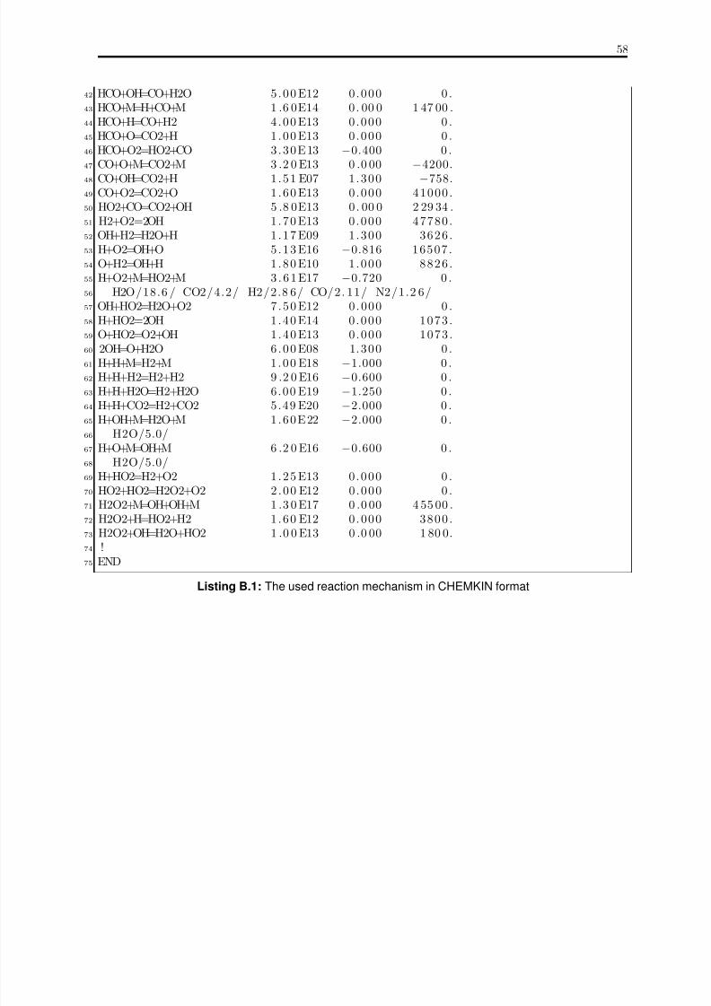
7/18/2019 120723_Bachelorthesis
http://slidepdf.com/reader/full/120723bachelorthesis 70/73
58
42 HCO+OH=CO+H2O 5 . 0 0 E12 0 . 0 0 0 0 .43 HCO+M=H+CO+M 1 .6 0E14 0 . 00 0 1 47 00 .44 HCO+H=CO+H2 4 . 0 0 E13 0 . 0 0 0 0 .45 HCO+O=CO2+H 1 . 0 0 E13 0 . 0 0 0 0 .46 HCO+O2=HO2+CO 3 . 3 0 E 13 −0.400 0 .47 CO+O+M=CO2+M 3 .2 0 E13 0 .0 00
−4200.
48 CO+OH=CO2+H 1 . 5 1 E07 1 . 3 0 0 −758.49 CO+O2=CO2+O 1 . 6 0 E13 0 . 0 0 0 4 1 0 0 0 .50 HO2+CO=CO2+OH 5 .8 0E13 0 . 00 0 2 29 34 .51 H2+O2=2OH 1 . 7 0 E13 0 . 0 0 0 4 7 7 8 0 .52 OH+H2=H2O+H 1 . 1 7 E09 1 . 3 0 0 3 6 2 6 .53 H+O2=OH+O 5 . 1 3 E16 −0.816 1 6 5 0 7 .54 O+H2=OH+H 1 . 8 0 E10 1 . 0 0 0 8 8 2 6 .55 H+O2+M=HO2+M 3 . 6 1 E17 −0.720 0 .56 H2O/18.6 / CO2/4.2/ H2/2.8 6/ CO/2. 11/ N2/1.2 6/57 OH+HO2=H2O+O2 7 . 5 0 E12 0 . 0 0 0 0 .58 H+HO2=2OH 1 . 4 0 E14 0 . 0 0 0 1 0 7 3 .59 O+HO2=O2+OH 1 . 4 0 E13 0 . 0 0 0 1 0 7 3 .
60 2OH=O+H2O 6 . 0 0 E08 1. 3 0 0 0 .61 H+H+M=H2+M 1 . 0 0 E18 −1.000 0 .62 H+H+H2=H2+H2 9 .2 0 E16 −0.600 0 .63 H+H+H2O=H2+H2O 6 . 0 0 E19 −1.250 0 .64 H+H+CO2=H2+CO2 5 . 4 9 E20 −2.000 0 .65 H+OH+M=H2O+M 1 . 6 0 E 22 −2.000 0 .66 H2O/5.0/67 H+O+M=OH+M 6 .2 0 E16 −0.600 0 .68 H2O/5.0/69 H+HO2=H2+O2 1 . 2 5 E13 0 . 0 0 0 0 .70 HO2+HO2=H2O2+O2 2 . 0 0 E12 0 . 0 0 0 0 .71 H2O2+M=OH+OH+M 1 .3 0 E17 0 .0 00 4 55 00 .72 H2O2+H=HO2+H2 1 . 6 0 E12 0 . 0 0 0 3 8 0 0 .73 H2O2+OH=H2O+HO2 1 .0 0 E13 0 .0 00 1 80 0.74 !75 END
Listing B.1: The used reaction mechanism in CHEMKIN format
7/18/2019 120723_Bachelorthesis
http://slidepdf.com/reader/full/120723bachelorthesis 71/73
Bibliography[1] R. J. Kee, M. E. Coltrin, and P. Glarborg. Chemically reacting flow : theory and
practice . Hoboken, NJ: Wiley Interscience, 2003.
[2] World energy outlook . Paris, 2010.
[3] S. R. Turns. An introduction to combustion: concepts and applications . McGraw-Hill series in mechanical engineering. Boston: McGraw-Hill, 2000.
[4] N. Peters. Turbulent combustion . Cambridge monographs on mechanics. Cam-bridge: Cambridge University Press, 2000.
[5] E. O. Lawrence. “Mixing and chemical reactions in turbulent flow reactors”. PhDthesis. University of California, 1964.
[6] T. Echekki, ed. Turbulent combustion modeling : advances, new trends and per-spectives . Fluid mechanics and its applications ; 95. Springer, 2011.
[7] M. Ferziger J. H. ; Perić. Numerische Strömungsmechanik . Berlin: Springer, 2008.
[8] J. H. Chen. “Petascale direct numerical simulation of turbulent combustion”. In:Proceedings of the Combustion Institute 33 (2011), pp. 99–123.
[9] C. Cabrit and F. Nicoud. “Direct simulations for wall modeling of multicomponentreacting compressible turbulent flows”. In: Physics of Fluids 21.055108 (2009).
[10] J. Warnatz, U. Maas, and R. W. Dibble. Combustion : physical and chemical fundamentals, modeling and simulation, experiments, pollutant formation . Berlin:Springer, 2006.
[11] M. Désilets, P. Proulx, and G. Soucy. “Modeling of multicomponent diffusion inhigh temperature flows”. In: International Journal of Heat and Mass Transfer 40.18 (1997), pp. 4273 –4278.
[12] J. Keller. “Influence of Molecular Diffusion Flux Modeling on the Structure of Non-Premixed and Partially Premixed Flames”. MA thesis. Technische UniversitätBergakademie Freiberg, 2011.
[13] A. Spille-Kohoff, E. Preuß, and K. Böttcher. “Numerical solution of multi-componentspecies transport in gases at any total number of components”. In: International Journal of Heat and Mass Transfer 55.19–20 (2012), pp. 5373 –5377.
[14] A. W. Cook. “Enthalpy diffusion in multicomponent flows”. In: Physics of Fluids 21.055109 (2009).
[15] H. Jasak, A. Jemcov, and Z. Tukovic. “OpenFOAM: A C++ Library for ComplexPhysics Simulations”. In: International Workshop on Coupled Methods in Numer-ical Dynamics . 2007.
7/18/2019 120723_Bachelorthesis
http://slidepdf.com/reader/full/120723bachelorthesis 72/73
Bibliography 60
[16] G. Dixon-Lewis. “Flame Structure and Flame Reaction Kinetics. II. TransportPhenomena in Multicomponent Systems”. In: Proceedings of the Royal Society of London. Series A, Mathematical and Physical Sciences 307 (1986), pp. 111–135.
[17] D. Goodwin. Cantera: Object-oriented software for reacting flows . September 2012.url: \\http://code.google.com/p/cantera/.
[18] M. Rehm. “Numerische Strömungssimulation der Hochdruckvergasung unter Berück-sichtigung detaillierter Reaktionsmechanismen”. PhD thesis. Technische Univer-sität Bergakademie Freiberg, 2010.
[19] R. B. Bird, W. E. Stewart, and E. N. Lightfoot. Transport phenomena . New York:Wiley, 2002.
[20] F.M. Rupley, R.J. Kee, and J.A. Miller. “PREMIX: A Fortran Program for Mod-eling Steady Laminar One-dimensional Premixed Flames”. In: Sandia National Laboratories Tech. Report SAND85-8240 (1995).
[21] T. Poinsot and D. Veynante. Theoretical and numerical combustion . Philadelphia,PA: Edwards, 2001.
[22] S. B. Pope. Turbulent flows . Cambridge University Press, 2000.
[23] L. P. H. de Goey and J. H. M. ten Thije Boonkkamp. “A Mass-Based Definitionof Flame Stretch for Flames with Finite Thickness”. In: Combustion Science and Technology 122.1-6 (1997), pp. 399–405.
[24] R. Brdička. Grundlagen der physikalischen Chemie . Berlin: Dt. Verl. d. Wiss.,1977.
[25] J. O. Hirschfelder, C. F. Curtiss, and R. B. Bird. Molecular theory of gases and
liquids . Structure of matter series. New York [u.a.]: Wiley [u.a.], 1954.[26] S. Chapman and T. G. Cowling. The Mathematical theory of non-uniform gases :
an account of the kinetic theory of viscosity, thermal conduction and diffusion in gases . Cambridge: Univ.Pr., 1970.
[27] M. Frenklach et al. “GRI-Mech - An Optimized Detailed Chemical Reaction Mech-anism for Methane Combustion”. In: Gas Research Institute Topical Report GRI-95/0058 (1995).
[28] C. R. Wilke. “A Viscosity Equation for Gas Mixtures”. In: The Journal of Chemical Physics 18 (1950), pp. 517–519.
[29] J. I. Steinfeld, J. S. Francisco, and W. L. Hase. Chemical kinetics and dynamics .Englewood Cliffs, NJ: Prentice Hall, 1989.
[30] H.-P. Schmid. “Ein Verbrennungsmodell zur Beschreibung der Wärmefreisetzungvon vorgemischten turbulenten Flammen”. PhD thesis. Universität Karlsruhe (TH),1995.
[31] OpenFOAM - The Open Source CFD Toolbox, Programmer’s Guide . 2.1.0. Open-FOAM Foundation. 2011.
[32] OpenFOAM - The Open Source CFD Toolbox, User Guide . 2.1.1. OpenFOAMFoundation. 2012.

7/18/2019 120723_Bachelorthesis
http://slidepdf.com/reader/full/120723bachelorthesis 73/73
Bibliography 61
[33] D. G. Goodwin. Cantera C++ User’s Guide . California Institute of Technology.2002.
[34] Regents of the University of California. BSD 3-Clause License . September 2012.url: http://opensource.org/licenses/BSD-3-Clause.
[35] R.J. Kee et al. CHEMKIN-III: A FORTRAN chemical kinetics package for the analysis of gas-phase chemical and plasma kinetics . Tech. rep. SAND96-8216. San-dia National Laboratories Report, 1996.
[36] B. Stroustrup. The C++ programming language . Boston [u.a.]: Addison-Wesley,2009.
[37] Scott Meyers. Effective C++ : 55 specific ways to improve your programs and designs . Addison-Wesley professional computing series. Upper Saddle River, NJ:Addison-Wesley, 2007.
[38] R. J. Kee et al. Tech. rep. SAND85-8240. Sandia National Laboratories Report,
1985.[39] K.J. Bosschaart and L.P.H. de Goey. “The laminar burning velocity of flames
propagating in mixtures of hydrocarbons and air measured with the heat fluxmethod”. In: Combustion and Flame 136 (2004), pp. 261–269.
[40] Cray XE6 . Cray Inc. 2010.
[41] M. Klein, A. Sadiki, and J. Janicka. “A digital filter based generation of inflow datafor spatially developing direct numerical or large eddy simulations”. In: Journal of Computational Physics 186 (2003), pp. 652–665.
[42] B. Krischok. Cray XE6 (HERMIT). 2012. url: http://www.hlrs.de/systems/
platforms/cray-xe6-hermit/.[43] D. Parkinson. “Parallel efficiency can be greater than unity”. In: Parallel Comput-
ing 3 (1986), pp. 261–262.