ac circuit
DESCRIPTION
BASIC AC CIRCUIT explanationTRANSCRIPT

ESE211 Lecture 3
Phasor Diagram of an RC Circuit
V(t)=Vm sin(ωt) R
Vi(t) C Vo(t)
• Current is a reference in series circuit
KVL: Vm = VR + VC
VR
Vm
Im ϕ
VC

ESE211 Lecture 3
Phasor Diagram of an RL Circuit
V(t)=Vmsin(ωt) VR (t) R
Vi(t) L Vo(t)
KVL: Vm = VR + VL
Vm
ϕ
VL
Im VR

ESE211 Lecture 3
Phasor Diagram of a Series RLC Circuit
VC VL
C L
Vi R VR
KVL: Vm = VC + VL + VR
VL
Vm
VL-C
VR Im
VC
• Voltages across capacitor and inductor compensate each other

ESE211 Lecture 4
Integrating Circuit
VR Vi(t) R Vo(t) C
V V Vi R= + C or V V Vi R= +2 2
C
• Assume high frequency 1/ωC << R then VR >> VC V VR i≈
V CI dt
RCV dtO i
t
i
t
= ≈∫ ∫1 1
0 0
Vi
V V dtO i∝ ∫
• Accurate integrating can be obtained at high
frequency that leads to a low output signal

ESE211 Lecture 4
Differentiating Circuit
VC Vi(t) C Vo(t) R
V V Vi R= + C or V V Vi R= +2 2
C
• Assume low frequency 1/ωC >> R then VR << VC VR
Vi V V C i≈ VC
I dt I Cddt
Vi i
t
i i≈ ⇒ =∫1
0
V V I R RCddt
VO R i i= = ≈
V
ddt
VO i∝
• An accurate result can be achived at low frequency.

ESE211 Lecture 4
Transient Processes
in Passive Circuits
RC Circuit without a Source
• The circuit response is due only to the energy stored in the
capacitor
t=0
C R
• The capacitor C is precharged to the voltage V0 Applying KCL:
C dV/dt +V/R = 0 • This is the 1st order differential equation

ESE211 Lecture 4
Solution of the Differential Equation
dV/dt + V/RC = 0
dV/V = -dt/RC
ln V = -t/RC +a
V = A e -t/RC , A=e+a • e is the base of the natural logarithms, e = 2.718…
• Continuity requires the initial condition:
At t = 0 V(0) = V0
V(t) = V0 e -t/RC
• The response governed by the elements themselves
without external force is called a natural response
ESE211 Lecture 4
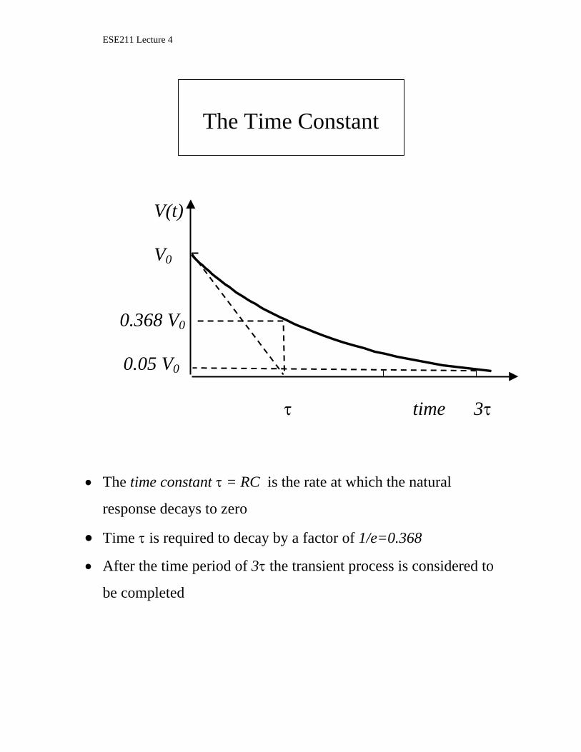
The Time Constant V(t)
V0
0.368 V0 0.05 V0
τ time 3τ
• The time constant τ = RC is the rate at which the natural
response decays to zero
• Time τ is required to decay by a factor of 1/e=0.368 • After the time period of 3τ the transient process is considered to
be completed
ESE211 Lecture 4
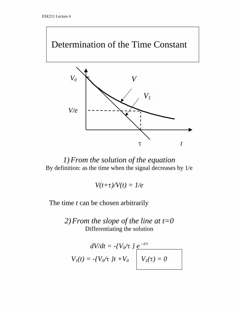
Determination of the Time Constant
V0 V/e τ t
V1
V
1) From the solution of the equation
By definition: as the time when the signal decreases by 1/e
V(t+τ)/V(t) = 1/e
The time t can be chosen arbitrarily
2) From the slope of the line at t=0 Differentiating the solution
dV/dt = -{V0/τ } e –t/τ
V1(t) = -{V0/τ }t +V0 V1(τ) = 0
ESE211 Lecture 4
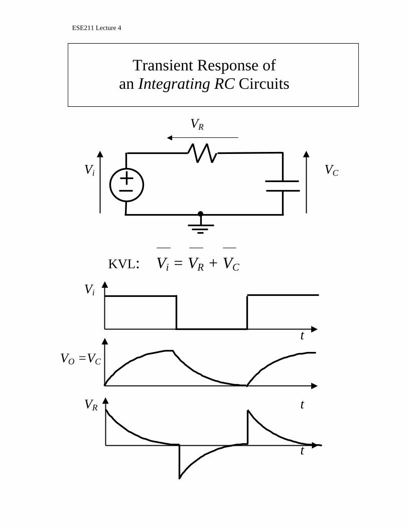
Transient Response of an Integrating RC Circuits
VR
Vi VC
KVL: Vi = VR + VC
Vi
t
VO =VC
VR t
t

ESE211 Lecture 4
Transient Response of a Differentiating RC Circuits
VC
Vi VR
KVL: Vi = VC + VR
Vi
t
VO = VR
t
VC

ESE211 Lecture 5
Transfer Function Vi(t) Vo(t) Vi(t) = Vimcos(ωt) Vo(t) = Vomcos(ωt+ϕ)
Vom(ω) ϕ(ω) Vo(t) =Re { Vo e jωt}, Vo = Vome jϕ
i
o
VVT )()( ω
ω =
Amplitude response |T(ω)| = Vom(ω)/Vim
Phase response ∠T(ω) = ϕ(ω)

ESE211 Lecture 5
The Transfer Function of
an Integrating RC Circuit R Vi(t) C Vo(t)
RCjCj
R
CjV
VTi
o
ωω
ωωω
+=
+==
11
1
1)()(
ωτω
jT
+=
11)(
τ = RC

ESE211 Lecture 5
-3 -2 -1 0 1 2 30.0
0.5
1.0
1000ωο100ωο
10ωοωο0.1ωο
0.01ωο0.001ωο
0.707
1000ωο100ωο10ωοωο0.1ωο
0.01ωο0.001ωο
|Vo/V
in|
Frequency (ω)
-3 -2 -1 0 1 2 310-3
10-2
10-1
100 slope-20 dB/dec-3 dB
Frequency (ω)
|Vo/V
in|
-60
-40
-20
0
V 0 [dB]
2211)(
τωω
+=T
Amplitude Response of
the Integrating RC Circuit
• The magnitude of the transfer function is
• The Integrating RC circuit is a LOW-PASS filter

ESE211 Lecture 5
-3 -2 -1 0 1 2 3
-90
-45
0
1000 ω ο 100 ω ο 10 ω ο ω ο 0.1 ω ο 0.01 ω ο 0.001 ω ο
V o
Frequency ( ω )
[ ][ ])(Re
)(Imarctan)(ωω
ωTTT =∠
)arctan()1)(1(
1)( ωτωτωτ
ωτω −=
−+−
∠=∠jj
jT
Phase Response of
the Integrating RC Circuit
The angle of the transfer function is

ESE211 Lecture 5
The Transfer Function of
a Differentiating RC Circuit C Vi(t) R Vo(t)
)()()()()(
ωωωω
ωRCi
o
XIRI
VVT
⋅⋅
==
RCjRCj
CjR
RX
RTRC ω
ω
ωω
ω+
=+
==11)(
)(
2222 1)(
1)1()(
τωωτωτ
τωωτωτ
ω+
+=
+−
=jjjT
τ = RC

ESE211 Lecture 5
-3 -2 -1 0 1 2 30.0
0.5
1.0
1000ωο100ωο
10ωοωο0.1ωο
0.01ωο0.001ωο
V0=0.707 V
in
1000ωο100ωο
10ωοωο
0.1ωο0.01ωο
0.001ωο
|V
o/Vin|
Frequency ( ω)
-3 -2 -1 0 1 2 310-3
10-2
10-1
100
slope-20 dB/dec
or-6 dB/oct
-3 dB point at ω0
Frequency ( ω)
|V
o/Vin|
-60
-40
-20
0
V 0 [dB]
222211
)()(τω
ωττω
ωτωτω
+=
++
=jT
Amplitude response of the Differentiating
RC Circuit
• Amplitude response of the RC circuit is the magnitude of T(ω)
• The Differentiating RC circuit is a HIGH-PASS filter

ESE211 Lecture 5
-3 -2 -1 0 1 2 3
0
45
90
1000ωο100ωο10ωοωο0.1ωο0.01ωο
0.001ωο
V 0
Frequency ( ω)
++
∠=∠ 221)()(
τωωτωτ
ωjT
ωτω
1arctan)( =∠T
Phase response of the Differentiating
RC Circuit
• Phase response of the RC circuit is the phase angle of T(ω)

ESE211 Lecture 5
Frequency Response of a Series RLC Circuit
VC VL
C L
Vi R VR
KVL: Vi = VC + VL + VR
VL
VL-C
VR Im
VC
Vi
• Voltages across capacitor and inductor compensate each other

ESE211 Lecture 5
-3 -2 -1 0 1 2 30.0
0.5
1.0
1000ωο100ωο10ωοωο0.1ωο0.01ωο0.001ωο
V0=0.707 Vin
1000ωο100ωο10ωοωο0.1ωο0.01ωο0.001ωο
|Vo/V
in|
Frequency ( ω)
-3 -2 -1 0 1 2 30.0
0.5
1.0
1.5
|VL/Vin||VC/Vin|
Frequency (ω)
|VC/
V in|,
|VL/V
in|
22
0
11|/|
−+
=++
=
CLR
R
RCj
Lj
RVV IN
ωωω
ω
Amplitude Response of a Series RLC Circuit

ESE211 Lecture 5
-3 -2 -1 0 1 2 3
-180
-90
0
1000 ωο100ωο10ωοωο0.1ωο0.01ωο0.001ωο
V o
Frequency (ω)
-3 -2 -1 0 1 2 310-6
10-4
10-2
100
slope-40 dB/dec
|Vo/V
in|
-120
-80
-40
0
V 0 [dB]
Amplitude and Phase Response of
the Ladder RC Circuit R R Vin C C Vo
1000ωο100ωο10ωοωο0.1ωο0.01ωο0.001ωο Frequency (ω)
ESE211 Lecture 5
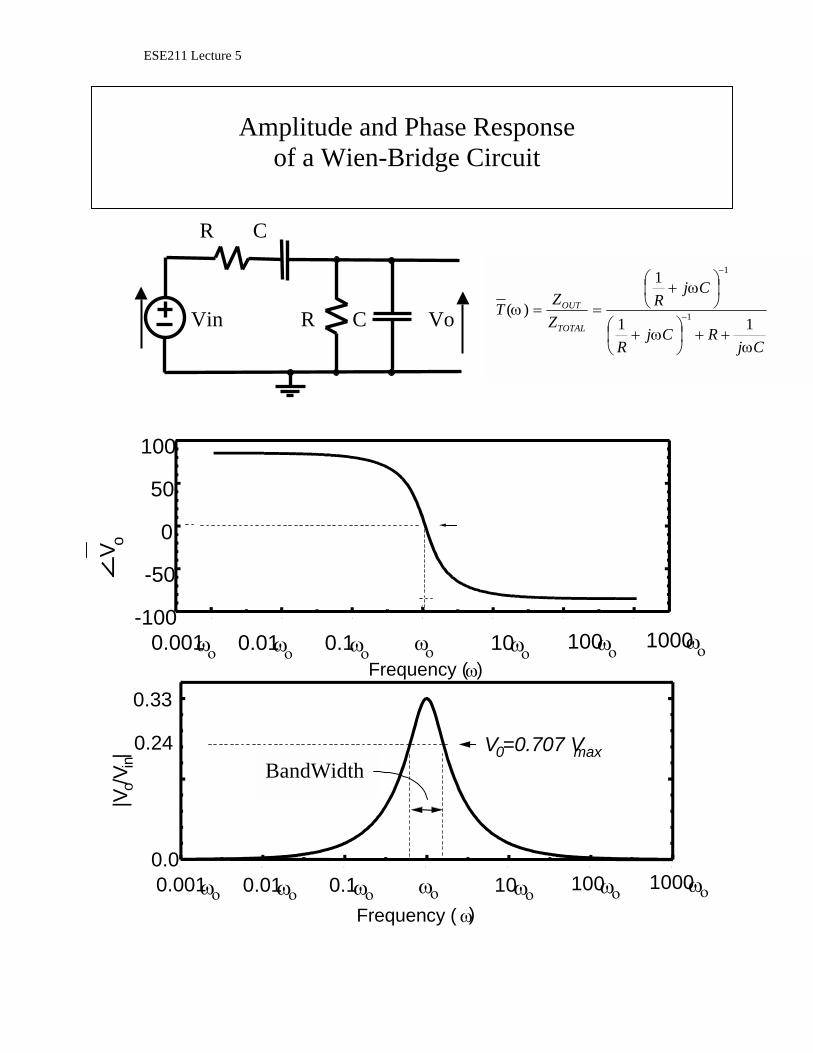
Amplitude and Phase Response of a Wien-Bridge Circuit
R C
BandWidth
-3 -2 -1 0 1 2 30.0
0.33
V0=0.707 Vmax
1000ωο100ωο10ωοωο0.1ωο0.01ωο0.001ωο
|V/V
|
Frequency ( ω)
0.245
o
in
Vin R C Vo Cj
RCjR
CjR
ZZT
TOTAL
OUT
ωω
ωω
11
1
)( 1
1
++
+
+
== −
−
Frequency (
-3 -2 -1 0 1 2 3 -100
0.001 ω ο
-50
0
50
100
V o
1000 ω ο 100 ω ο 0.01 ω ο 0.1 ω ο 10 ω ο ω ο ω )