07 Multivariate models: Granger causality, VARand VECM models

Andrius Buteikis, andrius.buteikis@mif.vu.lthttp://web.vu.lt/mif/a.buteikis/

Introduction

In the present chapter, we discuss methods which involve more than oneequation. To motivate why multiple equation methods are important, webegin by discussing Granger causality. Later, we move to discussing themost popular class of multiple-equation models: so-called VectorAutoregressive (VAR) models. VARs can be used to investigate Grangercausality, but are also useful for many other things in finance.

Time series models for integrated series are usually based on applyingVAR to first differences. However, differencing eliminates valuableinformation about the relationship among integrated series - this is whereVector Error Correction model (VECM) is applicable.

Granger CausalityIn our discussion of regression, we were on a little firmer ground, since weattempted to use common sense in labeling one variable the dependentvariable and the others the explanatory variables. In many cases, becausethe latter ‘explained’ the former it was reasonable to talk about X‘causing’ Y. For instance, the price of the house can be said to be‘caused’ by the characteristics of the house (e.g., number of bedrooms,number of bathrooms, etc.).

However, one can run a regression of Y = stock prices in Country B on X= stock prices in Country A. It is possible that stock price movements inCountry A cause stock markets to change in Country B (i.e., X causes Y). For instance, if Country A is a big country with an important role inthe world economy (e.g., the USA), then a stock market crash in CountryA could also cause panic in Country B. However, if Country A and Bwere neighboring countries (e.g., Thailand and Malaysia) then an eventwhich caused panic in either country could affect both countries.

In other words, the causality could run in either direction - or both!Hence, when using the word ‘cause’ with regression or correlation resultsa great deal of caution has to be taken and common sense has to be used.

However, with time series data we can make slightly stronger statementsabout causality simply by exploiting the fact that time does not runbackward! That is, if event A happens before event B, then it is possiblethat A is causing B. However, it is not possible that B is causing A. Inother words, events in the past can cause events to happen today. Futureevents cannot.

These intuitive ideas can be investigated through regression modelsincorporating the notion of Granger or regressive causality. The basicidea is that a variable X Granger causes Y if past values of X can helpexplain Y.

Of course, if Granger causality holds this does not guarantee that Xcauses Y. This is why we say ‘Granger causality’ rather than just‘causality’. Nevertheless, if past values of X have explanatory power forcurrent values of Y, it at least suggests that X might be causing Y.

Granger causality is only relevant with time series variables.

To illustrate the basic concepts we will consider Granger causalitybetween two variables (X and Y ) which are both stationary. Anonstationary case, where X and Y have unit roots but are cointegrated,will be mentioned below. Since X and Y are both stationary, an ADLmodel is appropriate. Suppose that the following simple ADL (only lagson the right hand side!) model holds:

Yt = α + φYt−1 + β1Xt−1 + εt

This model implies that last period’s value of X has explanatory powerfor the current value of Y . The coefficient β1 is a measure of theinfluence of Xt−1 on Yt . If β1 = 0, then past values of X have no effecton Y and there is no way that X could Granger cause Y.

In other words, if β1 = 0 then X does not Granger cause Y.

Since we know how to estimate the ADL and carry out hypothesis tests,it is simple to test Granger causality or, in other words, to testH0 : β1 = 0: if β1 is statistically significant (i.e. its p − value < 0.05 ),then we conclude that X Granger causes Y. Note that the null hypothesisbeing tested here is hypothesis that Granger causality does not occur.We will refer to this procedure as a Granger causality test.

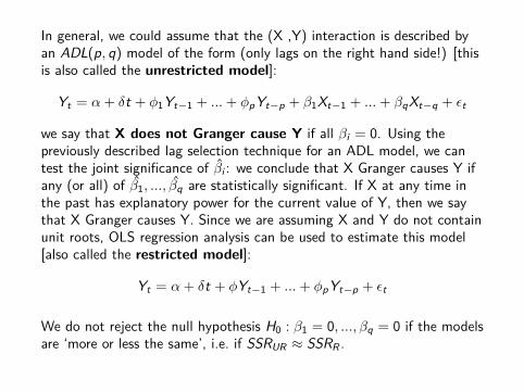
In general, we could assume that the (X ,Y) interaction is described byan ADL(p, q) model of the form (only lags on the right hand side!) [thisis also called the unrestricted model]:

Yt = α + δt + φ1Yt−1 + ...+ φpYt−p + β1Xt−1 + ...+ βqXt−q + εt

we say that X does not Granger cause Y if all βi = 0. Using thepreviously described lag selection technique for an ADL model, we cantest the joint significance of βi : we conclude that X Granger causes Y ifany (or all) of β1, ..., βq are statistically significant. If X at any time inthe past has explanatory power for the current value of Y, then we saythat X Granger causes Y. Since we are assuming X and Y do not containunit roots, OLS regression analysis can be used to estimate this model[also called the restricted model]:

Yt = α + δt + φYt−1 + ...+ φpYt−p + εt

We do not reject the null hypothesis H0 : β1 = 0, ..., βq = 0 if the modelsare ‘more or less the same’, i.e. if SSRUR ≈ SSRR .

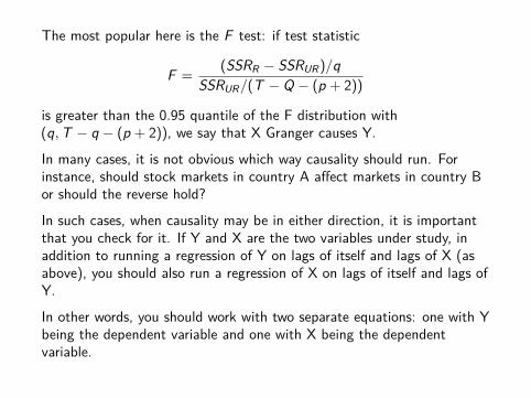
The most popular here is the F test: if test statistic

F = (SSRR − SSRUR)/qSSRUR/(T − Q − (p + 2))

is greater than the 0.95 quantile of the F distribution with(q,T − q − (p + 2)), we say that X Granger causes Y.

In many cases, it is not obvious which way causality should run. Forinstance, should stock markets in country A affect markets in country Bor should the reverse hold?

In such cases, when causality may be in either direction, it is importantthat you check for it. If Y and X are the two variables under study, inaddition to running a regression of Y on lags of itself and lags of X (asabove), you should also run a regression of X on lags of itself and lags ofY.

In other words, you should work with two separate equations: one with Ybeing the dependent variable and one with X being the dependentvariable.

This brief discussion of Granger causality has focused on two variables, Xand Y . However, there is no reason why these basic techniques cannotbe extended to the case of many variables.

For instance, if we had three variables, X , Y and Z , and were interestedin investigating whether X or Z Granger cause Y, we would simply regressY on lags of Y , lags of X and lags of Z .

If, say, the lags of Z were found to be significant and the lags of X not,then we could say that Z Granger causes Y, but X does not.

Testing for Granger causality among cointegrated variables is verysimilar to the method outlined above. Remember that, if variables arefound to be cointegrated (something which should be investigated usingunit root and cointegration tests), then you should work with an errorcorrection model (ECM) involving these variables. In the case where youhave two variables, this is given by:

∆Yt = φ+δt+λet−1+γ1∆Yt−1+...+γp∆Yt−p+ω1∆Xt−1+...+ωq∆Xt−q+εt

This is essentially an ADL model except for the presence of the termλet−1, where et−1 = Yt−1 − α− βXt−1.

X Granger causes Y if past values of X have explanatory power forcurrent values of Y. Applying this intuition to the ECM, we can see thatpast values of X appear in the terms ∆Xt−1, ...,∆Xt−q and et−1. Thisimplies that X does not Granger cause Y if ω1 = ... = ωq = λ = 0.

t-statistics and p-values can be used to test for Granger causality in thesame way as the stationary case. Also, the F - tests can be used to carryout a formal test of H0 : ω1 = ... = ωq = λ = 0

The bottom line - if X Granger-causes Y , this does not mean thatX causes Y , it only means that X improves Y ’s predictability (i.e.,reduces residuals of the model).

VAR: Estimation and forecasting

Our discussion of Granger causality naturally leads us to an interest inmodels with several equations and the topic of Vector Autoregressionsor VARs.

Initially, we will assume that all variables are stationary. If the originalvariables have unit roots, then we assume that differences have beentaken such that the model includes the changes in the original variables(which do not have unit roots). The end of this section will consider theextension of this case to that of cointegration.

When we investigated Granger causality between X and Y, we began withan ADL(p, q) model for Y as the dependent variable. We used it toinvestigate if X Granger caused Y. We then went on to consider causalityin the other direction, which involved switching the roles of X and Y inthe ADL. In particular, X became the dependent variable. We can writethe two equations as follows:

Yt = α1 + δ1t + φ11Yt−1 + ...+ φ1pYt−p + β11Xt−1 + ...+ β1qXt−q + ε1t

Xt = α2 + δ2t + φ21Yt−1 + ...+ φ2pYt−p + β21Xt−1 + ...+ β2qXt−q + ε2t

The first of these equations tests whether X Granger causes Y; thesecond, whether Y Granger causes X. Note that now the coefficients havesubscripts indicating which equation they are in. The errors now havesubscripts to denote the fact that they will be different in the twoequations.

These two equations comprise a VAR. A VAR is the extension of theautoregressive (AR) model to the case in which there is more than onevariable under study. A VAR has more than one dependent variable (e.g.,Y and X ) and, thus, has more than one equation. Each equation uses asits explanatory variables lags of all the variables under study (andpossibly a deterministic trend).

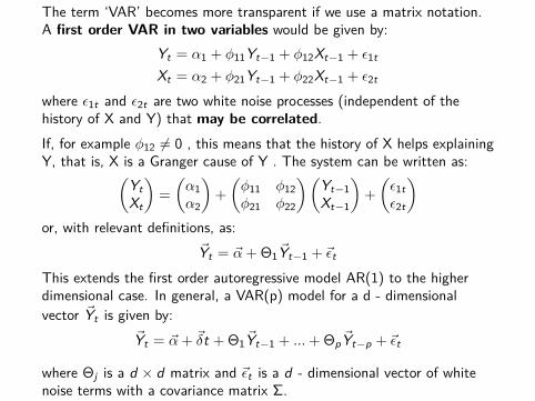
The term ‘VAR’ becomes more transparent if we use a matrix notation.A first order VAR in two variables would be given by:

Yt = α1 + φ11Yt−1 + φ12Xt−1 + ε1t

Xt = α2 + φ21Yt−1 + φ22Xt−1 + ε2t

where ε1t and ε2t are two white noise processes (independent of thehistory of X and Y) that may be correlated.If, for example φ12 6= 0 , this means that the history of X helps explainingY, that is, X is a Granger cause of Y . The system can be written as:(

YtXt

)=(α1α2

)+(φ11 φ12φ21 φ22

)(Yt−1Xt−1

)+(ε1tε2t

)or, with relevant definitions, as:

~Yt = ~α + Θ1~Yt−1 + ~εt

This extends the first order autoregressive model AR(1) to the higherdimensional case. In general, a VAR(p) model for a d - dimensionalvector ~Yt is given by:

~Yt = ~α + ~δt + Θ1~Yt−1 + ...+ Θp ~Yt−p + ~εt

where Θj is a d × d matrix and ~εt is a d - dimensional vector of whitenoise terms with a covariance matrix Σ.

Similarly to one-dimensional case, a VAR(p) is stationary if all the rootsof the equation det(Ik −Θ1z −Θ2z2 − ...−Θpzp) = 0 are outside a unitcomplex circle. The VAR is said to have a single unit root if the aboveequation has exactly one root z = +1, i.e.

det(Ik −Θ1 −Θ2 − ...−Θp) = 0

This will hold, if at least one of the variables in the VAR contains a unitroot.

Why we would want to work with such models? One reason has to beGranger causality testing. That is, VARs provide a framework for testingfor Granger causality between each set of variables.

Determining the lag length p in an empirical application is not alwayseasy and univariate autocorrelation or partial autocorrelation functionswill not help. A reasonable strategy is to estimate a VAR model fordifferent values of p and then select on the basis of the Akaike orSchwarz information criteria.

Once the order p has been established, we have to estimate thecoefficients. It appears that to get BLUE estimators, we can apply OLSto every equation individually (this is what, in R, VAR of the the packagevars or lineVar of the package tsDyn, do).

Below we shall examine forecasting a VAR(2) model, but at first wepresent a brief introduction to some of the practical issues and intuitiveideas relating to forecasting. All our discussion will relate to forecastingwith VARs but it is worth noting that the ideas also relate to forecastingwith univariate time series models. After all, an AR model is just a VARwith only one equation.

ForecastingForecasting is usually done using time series variables. The idea is thatyou use your observed data to predict what you expect to happen in thefuture. In more technical terms, you use data for periods t = 1, ...,T toforecast periods T + 1,T + 2, .... To provide some intuition for howforecasting is done, consider a VAR(1) involving two variables, Y and X:

Yt = α1 + δ1t + φ11Yt−1 + φ12Xt−1 + ε1t

Xt = α2 + δ2t + φ21Yt−1 + φ22Xt−1 + ε2t

You cannot observe YT +1 but you want to make a guess of what it islikely to be. Using the first equation of the VAR and setting t = T + 1,we obtain an expression for YT +1:

YT +1 = α1 + δ1(T + 1) + φ11YT + φ12XT + ε1,T +1

This equation cannot be directly used to obtain YT +1 since we don’tknow what unpredictable shock ε1,T +1 or surprise will hit the economynext period. Furthermore, we do not know what the coefficients are.

However, if we ignore the error term (which cannot be forecast since it isunpredictable) and replace the coefficients by their estimates we obtain aforecast which we denote as YT +1:

YT +1 = α1 + δ1(T + 1) + φ11YT + φ12XT

We can use the same strategy for two periods, provided that we makeone extension - since our data only runs until period T, we do not knowwhat YT +1 and XT +1 are. Consequently, we replace YT +1 and XT +1 byYT +1 and XT +1 (this called a dynamic forecast). The same can be doneto calculate XT +2:

YT +2 = α1 + δ1(T + 2) + φ11YT +1 + φ12XT +1

XT +2 = α2 + δ2(T + 2) + φ21YT +1 + φ22XT +1

We can use the general strategy of ignoring the error, replacingcoefficients by their estimates and replacing lagged values of variablesthat are unobserved by forecasts, to obtain forecasts for any number ofperiods in the future for any VAR(p).

VAR: Summary

Building a VAR model involves three steps:

1. use some information criterion to identify the order,2. estimate the specified model by using the least squares method and,

if necessary, re-estimate the model by removing statisticallyinsignificant parameters

3. use the Portmanteau test statistic of the residuals to check theadequacy of a fitted model (this is a multivariate analogue of theLjung-Box Q-stat in an ARIMA model and is to test forautocorrelation and cross-correlation in residuals). If the fittedmodel is adequate, then it can be used to obtain forecasts.

Example

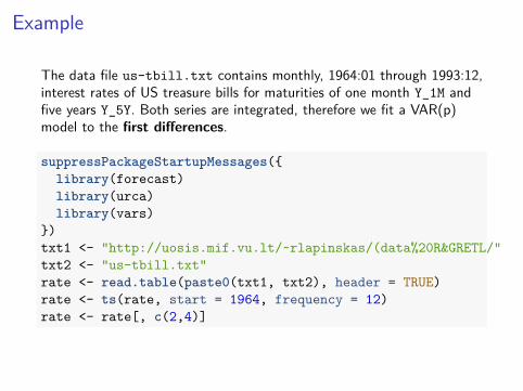
The data file us-tbill.txt contains monthly, 1964:01 through 1993:12,interest rates of US treasure bills for maturities of one month Y_1M andfive years Y_5Y. Both series are integrated, therefore we fit a VAR(p)model to the first differences.

suppressPackageStartupMessages({library(forecast)library(urca)library(vars)

})txt1 <- "http://uosis.mif.vu.lt/~rlapinskas/(data%20R&GRETL/"txt2 <- "us-tbill.txt"rate <- read.table(paste0(txt1, txt2), header = TRUE)rate <- ts(rate, start = 1964, frequency = 12)rate <- rate[, c(2,4)]

plot.ts(rate, main = "Interest rates of 1M & 5Y US T-bills")

24

68

1012

1416

Y_1

M

46

810

1214

1965 1970 1975 1980 1985 1990 1995

Y_5

Y

Time

Interest rates of 1M & 5Y US T−bills

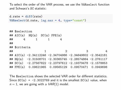
To select the order of the VAR process, we use the VARselect functionand Schwarz’s SC statistic:

d.rate = diff(rate)VARselect(d.rate, lag.max = 4, type="const")

## $selection## AIC(n) HQ(n) SC(n) FPE(n)## 4 1 1 4#### $criteria## 1 2 3 4## AIC(n) -2.34112246 -2.34704986 -2.34649802 -2.3542181## HQ(n) -2.31508701 -2.30365745 -2.28574864 -2.2761117## SC(n) -2.27567822 -2.23797612 -2.19379478 -2.1578853## FPE(n) 0.09621965 0.09565129 0.09570471 0.0949698

The $selection shows the selected VAR order for different statistics.Since SC(n) = -2.3022769 and it is the smallest SC(n) value, whenn = 1, we are going with a VAR(1) model.

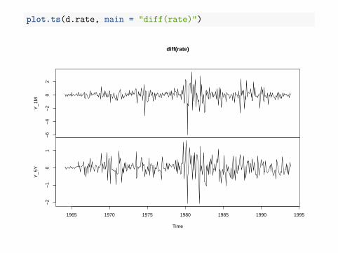
plot.ts(d.rate, main = "diff(rate)")

−6

−4

−2

02

Y_1

M

−2

−1

01

1965 1970 1975 1980 1985 1990 1995

Y_5

Y

Time

diff(rate)

Because d.rate does not have a drift, we will create a VAR modelwithout one:

var.diff = VAR(d.rate, p = 1, type = "none")coefficients(var.diff)

## $Y_1M## Estimate Std. Error t value Pr(>|t|)## Y_1M.l1 -0.2341646 0.05524366 -4.238760 2.867202e-05## Y_5Y.l1 0.6343748 0.10732304 5.910891 7.970641e-09#### $Y_5Y## Estimate Std. Error t value Pr(>|t|)## Y_1M.l1 -0.007842584 0.02987634 -0.2625015 0.7930866## Y_5Y.l1 0.074123953 0.05804140 1.2770876 0.2024036

We note that the estimation results show that Y_5Y is the Granger causeof Y_1M (in the 1st model the p-value of Y_5Y.l1 is < 0.05) but notvice versa (in the 2nd model the p-value of Y_5Y.l1 is > 0.05) (theR-squared is also larger in the 1st equation).

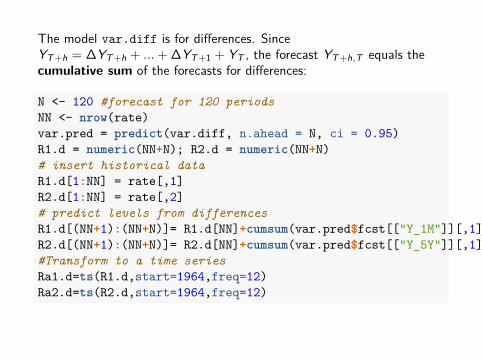
The model var.diff is for differences. SinceYT +h = ∆YT +h + ...+ ∆YT +1 + YT , the forecast YT +h,T equals thecumulative sum of the forecasts for differences:

N <- 120 #forecast for 120 periodsNN <- nrow(rate)var.pred = predict(var.diff, n.ahead = N, ci = 0.95)R1.d = numeric(NN+N); R2.d = numeric(NN+N)# insert historical dataR1.d[1:NN] = rate[,1]R2.d[1:NN] = rate[,2]# predict levels from differencesR1.d[(NN+1):(NN+N)]= R1.d[NN]+cumsum(var.pred$fcst[["Y_1M"]][,1])R2.d[(NN+1):(NN+N)]= R2.d[NN]+cumsum(var.pred$fcst[["Y_5Y"]][,1])#Transform to a time seriesRa1.d=ts(R1.d,start=1964,freq=12)Ra2.d=ts(R2.d,start=1964,freq=12)

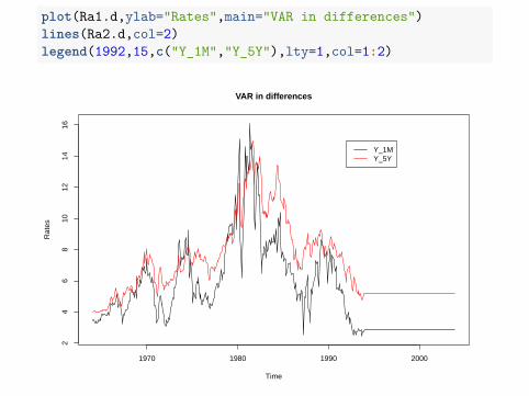
plot(Ra1.d,ylab="Rates",main="VAR in differences")lines(Ra2.d,col=2)legend(1992,15,c("Y_1M","Y_5Y"),lty=1,col=1:2)

VAR in differences

Time

Rat

es

1970 1980 1990 2000

24

68

1012

1416

Y_1MY_5Y

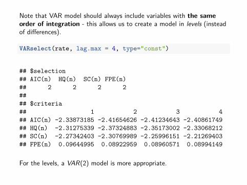
Note that VAR model should always include variables with the sameorder of integration - this allows us to create a model in levels (insteadof differences).

VARselect(rate, lag.max = 4, type="const")

## $selection## AIC(n) HQ(n) SC(n) FPE(n)## 2 2 2 2#### $criteria## 1 2 3 4## AIC(n) -2.33873185 -2.41654626 -2.41234643 -2.40861749## HQ(n) -2.31275339 -2.37324883 -2.35173002 -2.33068212## SC(n) -2.27342403 -2.30769989 -2.25996151 -2.21269403## FPE(n) 0.09644995 0.08922959 0.08960571 0.08994149

For the levels, a VAR(2) model is more appropriate.

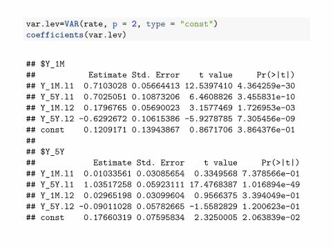
var.lev=VAR(rate, p = 2, type = "const")coefficients(var.lev)

## $Y_1M## Estimate Std. Error t value Pr(>|t|)## Y_1M.l1 0.7103028 0.05664413 12.5397410 4.364259e-30## Y_5Y.l1 0.7025051 0.10873206 6.4608826 3.455831e-10## Y_1M.l2 0.1796765 0.05690023 3.1577469 1.726953e-03## Y_5Y.l2 -0.6292672 0.10615386 -5.9278785 7.305456e-09## const 0.1209171 0.13943867 0.8671706 3.864376e-01#### $Y_5Y## Estimate Std. Error t value Pr(>|t|)## Y_1M.l1 0.01033561 0.03085654 0.3349568 7.378566e-01## Y_5Y.l1 1.03517258 0.05923111 17.4768387 1.016894e-49## Y_1M.l2 0.02965198 0.03099604 0.9566375 3.394049e-01## Y_5Y.l2 -0.09011028 0.05782665 -1.5582829 1.200623e-01## const 0.17660319 0.07595834 2.3250005 2.063839e-02

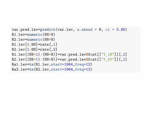
var.pred.lev=predict(var.lev, n.ahead = N, ci = 0.95)R1.lev=numeric(NN+N)R2.lev=numeric(NN+N)R1.lev[1:NN]=rate[,1]R2.lev[1:NN]=rate[,2]R1.lev[(NN+1):(NN+N)]=var.pred.lev$fcst[["Y_1M"]][,1]R2.lev[(NN+1):(NN+N)]=var.pred.lev$fcst[["Y_5Y"]][,1]Ra1.lev=ts(R1.lev,start=1964,freq=12)Ra2.lev=ts(R2.lev,start=1964,freq=12)

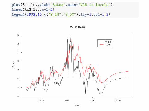
plot(Ra1.lev,ylab="Rates",main="VAR in levels")lines(Ra2.lev,col=2)legend(1992,15,c("Y_1M","Y_5Y"),lty=1,col=1:2)

VAR in levels

Time

Rat

es

1970 1980 1990 2000

24

68

1012

1416

Y_1MY_5Y

VAR in differences

Time

Rat

es

1970 1980 1990 2000

24

68

1012

1416

Y_1MY_5Y

VAR in levels

Time

Rat

es

1970 1980 1990 2000

24

68

1012

1416

Y_1MY_5Y

Both levels revert to (the values close to) their means (i.e. a stationarybehavior) which contradicts the unit root (i.e. non-stationary) behavior ofeach series. The explanation lies in the fact that we estimated anunrestricted VAR model while actually the coefficients should reflectcointegration and obey some constrains (this will be later discussed inthe VECM section).

VAR: Impulse-Response Function

The impulse-response function is yet another device that helps us tolearn about the dynamic properties of vector autoregressions of interestto forecasters. The question of interest is simple and direct: How does aunit innovation to a series affect it, now and in the future?

To clarify the issue, let us start with one-dimensional case. LetY1 = ... = YT−1 = 0, ε1 = ... = εT−1 = 0 and at moment t = T a unitshock comes: εT = σ, εT +1 = ... = 0.

I If Yt = εt , i.e. Yt is a WN, then YT = σ, YT +1 = εT +1 = 0 andYT +h = εT +h = 0 - WN has no memory, no dynamics;

I If Yt = φYt−1 + εt , |φ| < 1, i.e. Yt is an AR(1), thenYT = φ · 0 + σ = σ, YT +1 = φσ + 0 = φσ, …, YT +h = φhσ ash→∞ - the impulse response is dying down.

Now consider again the two-variable, first-order system:

Yt = φ11Yt−1 + φ12Xt−1 + ε1t

Xt = φ21Yt−1 + φ22Xt−1 + ε2t

I A perturbation in ε1t has an immediate one-for-one effect on Yt , butno effect on Xt .

I In period t + 1, that perturbation in Yt affects Yt+1 through the 1stequation, and also affects Xt+1, through the 2nd equation.

I These effects work through to period t + 2 etc.

Thus a perturbation in one innovation in the VAR sets up a chainreaction over time in all variables in the VAR. Impulse response functionscalculate these chain reactions.

Example (continued):The IRF (impulse-response function) can be calculated in R. The reactionto the unit Y_1M impulse:

plot(irf(var.diff, impulse = "Y_1M"))

xy$x

Y_1

M

0.0

0.2

0.4

0.6

0.8

xy$x

Y_5

Y

0.0

0.2

0.4

0.6

0.8

0 1 2 3 4 5 6 7 8 9 10

Orthogonal Impulse Response from Y_1M

95 % Bootstrap CI, 100 runs

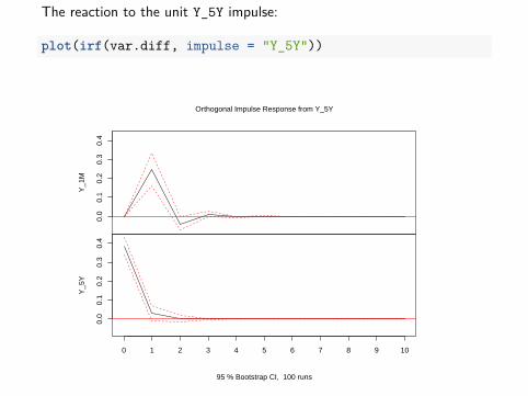
The reaction to the unit Y_5Y impulse:

plot(irf(var.diff, impulse = "Y_5Y"))

xy$x

Y_1

M

0.0

0.1

0.2

0.3

0.4

xy$x

Y_5

Y

0.0

0.1

0.2

0.3

0.4

0 1 2 3 4 5 6 7 8 9 10

Orthogonal Impulse Response from Y_5Y

95 % Bootstrap CI, 100 runs

Example 2Suppose our VAR(1) model is:

(YtXt

)=(

0.4 0.10.2 0.5

)(Yt−1Xt−1

)+(ε1,tε2,t

),

(ε1,tε2,t

)∼ N

((00

),

(16 1414 25

))We can show that this model is stationary:

det([

1 00 1

]−[0.4 0.10.2 0.5

]z)

= det([

1− 0.4z −0.1z−0.2z 1− 0.5z

])= 1− 0.5z − 0.4z + 0.2z2 − 0.02z2 = 0.18z2 − 0.9z + 1

# Find roots of equation: 1 - 0.9 * z + 0.18 * z^2 = 0roots <- polyroot(c(1, -0.9, 0.18))paste0("Absolute: |z_i| = ", round(abs(roots), 4))

## [1] "Absolute: |z_i| = 1.6667" "Absolute: |z_i| = 3.3333"

Because the roots are greater than one in absolute value, the VAR(1)process is stationary.

If we set:(Y0,X0) = (0, 0), ~ε1 = (4, 0)′, ~εj = 0, j > 1

i.e. initialize ~Yt values at zero and set a one-standard-deviationinnovation in the first equation and a zero innovation in the secondequation in period one and assume no further shocks from innovations.

The first few ~Yt values are:(Y1X1

)=(

40

),

(Y2X2

)= Θ1

(Y1X1

)+ ~ε2 =

(1.60.8

),

(Y3X3

)=(

0.720.72

)If we set:

(Y0,X0) = (0, 0), ~ε1 = (0, 5)′, ~εj = 0, j > 1Then:(

Y1X1

)=(

05

),

(Y2X2

)= Θ1

(Y1X1

)+ ~ε2 =

(0.52.5

),

(Y3X3

)=(

0.451.35

)An objection to the procedure just illustrated for the computation irf isthat the innovations in the VAR are, in general, not contemporaneouslyindependent of one another, i.e. the shock covariance matrix Σ is notdiagonal. So cases when one innovation receives a perturbation and theother does not is implausible. Ignoring this gives incorrect irf results!

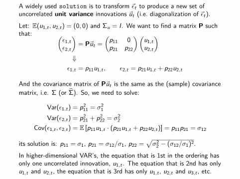
A widely used solution is to transform ~εt to produce a new set ofuncorrelated unit variance innovations ~ut (i.e. diagonalization of ~εt).

Let: E(u1,t , u2,t) = (0, 0) and Σu = I. We want to find a matrix P suchthat: (

ε1,tε2,t

)= P~ut =

(p11 0p21 p22

)(u1,tu2,t

)⇓

ε1,t = p11u1,t , ε2,t = p21u1,t + p22u2,t

And the covariance matrix of P~ut is the same as the (sample) covariancematrix, i.e. Σ (or Σ). So, we need to solve:

Var(ε1,t) = p211 = σ2

1

Var(ε2,t) = p221 + p2

22 = σ22

Cov(ε1,t , ε2,t) = E [p11u1,t · (p21u1,t + p22u2,t)] = p11p21 = σ12

its solution is: p11 = σ1, p21 = σ12/σ1, p22 =√σ2

2 − (σ12/σ1)2.

In higher-dimensional VAR’s, the equation that is 1st in the ordering hasonly one uncorrelated innovation, u1,t . The equation that is 2nd has onlyu1,t and u2,t , the equation that is 3rd has only u1,t , u2,t and u3,t , etc.

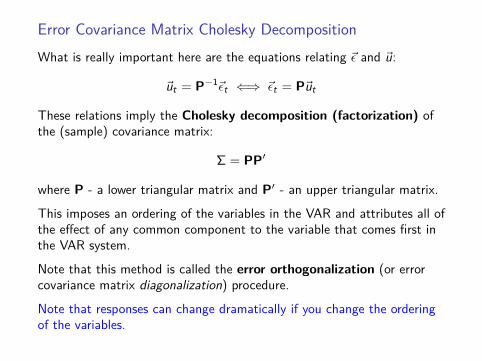
Error Covariance Matrix Cholesky DecompositionWhat is really important here are the equations relating ~ε and ~u:

~ut = P−1~εt ⇐⇒ ~εt = P~ut

These relations imply the Cholesky decomposition (factorization) ofthe (sample) covariance matrix:

Σ = PP′

where P - a lower triangular matrix and P′ - an upper triangular matrix.

This imposes an ordering of the variables in the VAR and attributes all ofthe effect of any common component to the variable that comes first inthe VAR system.

Note that this method is called the error orthogonalization (or errorcovariance matrix diagonalization) procedure.

Note that responses can change dramatically if you change the orderingof the variables.

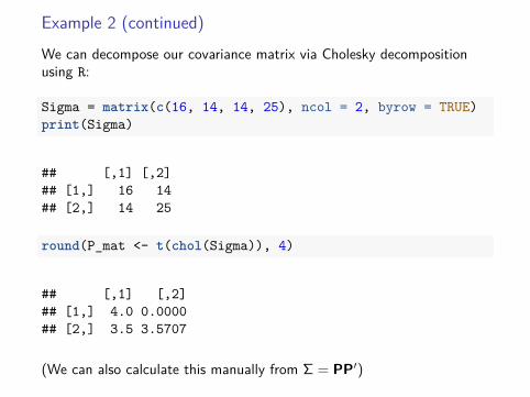
Example 2 (continued)

We can decompose our covariance matrix via Cholesky decompositionusing R:

Sigma = matrix(c(16, 14, 14, 25), ncol = 2, byrow = TRUE)print(Sigma)

## [,1] [,2]## [1,] 16 14## [2,] 14 25

round(P_mat <- t(chol(Sigma)), 4)

## [,1] [,2]## [1,] 4.0 0.0000## [2,] 3.5 3.5707

(We can also calculate this manually from Σ = PP′)

So:P =

(4 0

3.5 3.5707

)Suppose, that we postulate ~u1 = (1, 0)′ and ~uj = (0, 0)′, j > 1. Thisvector gives a one standard deviation perturbation in the first component.This results in:

~ε1 = P~u1 =(

4 03.5 3.5707

)(10

)=(

43.5

)So, the second element in ~ε1 is now non-zero compared to the case,where we ignored the non-diagonal nature of the error covariance matrix.

We can calculate the values ~Y1, ~Y2, ... as we did before.

Theta_1 = matrix(c(0.4, 0.1, 0.2, 0.5), ncol = 2, byrow = TRUE)#Y_1:print(Y_1 <- P_mat %*% c(1, 0))

## [,1]## [1,] 4.0## [2,] 3.5

#Y_2:print(Y_2 <- Theta_1 %*% Y_1)

## [,1]## [1,] 1.95## [2,] 2.55

#Y_3:print(Y_3 <- Theta_1 %*% Y_2)

## [,1]## [1,] 1.035## [2,] 1.665

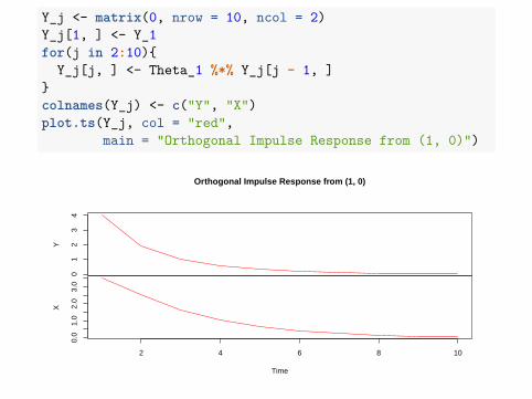
Y_j <- matrix(0, nrow = 10, ncol = 2)Y_j[1, ] <- Y_1for(j in 2:10){

Y_j[j, ] <- Theta_1 %*% Y_j[j - 1, ]}colnames(Y_j) <- c("Y", "X")plot.ts(Y_j, col = "red",

main = "Orthogonal Impulse Response from (1, 0)")

01

23

4

Y

0.0

1.0

2.0

3.0

2 4 6 8 10

X

Time

Orthogonal Impulse Response from (1, 0)

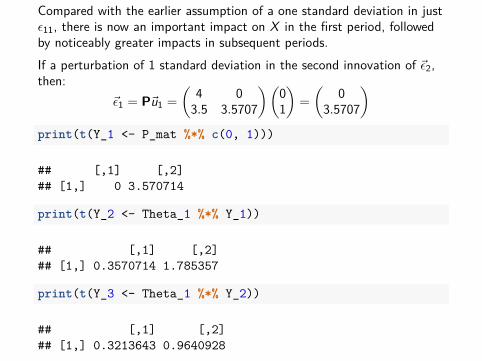
Compared with the earlier assumption of a one standard deviation in justε11, there is now an important impact on X in the first period, followedby noticeably greater impacts in subsequent periods.If a perturbation of 1 standard deviation in the second innovation of ~ε2,then:

~ε1 = P~u1 =(

4 03.5 3.5707

)(01

)=(

03.5707

)print(t(Y_1 <- P_mat %*% c(0, 1)))

## [,1] [,2]## [1,] 0 3.570714

print(t(Y_2 <- Theta_1 %*% Y_1))

## [,1] [,2]## [1,] 0.3570714 1.785357

print(t(Y_3 <- Theta_1 %*% Y_2))

## [,1] [,2]## [1,] 0.3213643 0.9640928

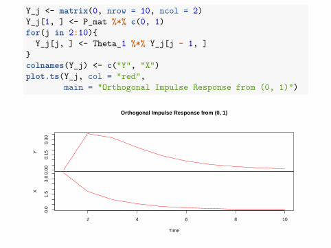
Y_j <- matrix(0, nrow = 10, ncol = 2)Y_j[1, ] <- P_mat %*% c(0, 1)for(j in 2:10){

Y_j[j, ] <- Theta_1 %*% Y_j[j - 1, ]}colnames(Y_j) <- c("Y", "X")plot.ts(Y_j, col = "red",

main = "Orthogonal Impulse Response from (0, 1)")

0.00

0.15

0.30

Y

0.0

1.5

3.0

2 4 6 8 10

X

Time

Orthogonal Impulse Response from (0, 1)

If we switch the variable order, so we have (Xt ,Yt), instead of (Yt ,Xt),then, because P is a lower triangular matrix, the effects also change:

Sigma = matrix(c(25, 14, 14, 16), ncol = 2, byrow = TRUE)round(P_mat <- t(chol(Sigma)), 4)

## [,1] [,2]## [1,] 5.0 0.0000## [2,] 2.8 2.8566

Theta_1 = matrix(c(0.5, 0.2, 0.1, 0.4), ncol = 2, byrow = TRUE)Y_1 <- P_mat %*% c(1, 0); Y_2 <- Theta_1 %*% Y_1Y_3 <- Theta_1 %*% Y_2print(cbind(Y_1, Y_2, Y_3))

## [,1] [,2] [,3]## [1,] 5.0 3.06 1.854## [2,] 2.8 1.62 0.954

Uncorrelated innovations were developed to deal with the problem ofnon-zero correlations between the original innovations.

However, the solution of one problem creates another. The new problemis that the order in which the ~u variables are entered can have dramaticeffects on the numerical results.

The interpretation of impulse response functions is thus a somewhathazardous operation, and there has been intense debate on their possibleeconomic significance.

One way to deal with it (for the case when P is the lower triangularmatrix) is to order with a decreasing order of exogeneity. That is, putfirst the equation with the largest number of exogenous variables, thenthe second, and so on, until you put last the variable, for which all theprevious variables have effect on it (i.e. the last variable has the leastamount of exogeneous variables).

The exogeneity property can also be formulated in terms of economictheory (i.e. which of the variables is the most and the least exogenous).

VECMRecall that the AR(p) process:

Yt = µ+ δt + φ1Yt−1 + φ2Yt−2 + ...+ φpYt−p + εt

can be rearranged into

∆Yt = µ+ δt + ρYt−1 + γ1∆Yt−1 + ...+ γp−1∆Yt−p+1 + εt

the latter form is more convenient for the unit root testing: H0 : ρ = 0implies that Yt has unit root. Similarly, the d - dimensional VAR process:

~Yt = ~µt + Θ1~Yt−1 + ...+ Θp ~Yt−p + ~εt

where ~µt = ~µ or ~µt = ~µ+ ~δt or ~µt = ~µ+ ~δt + ~γt2, can be rewritten inVEC form:

∆~Yt = ~µt + Π~Yt−1 + Γ1∆~Yt−1 + ...+ Γp−1∆~Yt−p+1 + ~εt

where the long-run matrix Π =∑p

i=1 Θi − I and Γi = −∑p

j=i+1 Θj .Note: if rank(Π) = r (i.e. r linearly independent cointegrating relations), it can be written as Πd×d = αd×rβ

Tr×d .

The rows of the matrix βT form a basis for the r cointegrating vectors and the elements of α distribute the impact of the cointegratingvectors to the evolution of ∆Yt (they are usually interpreted as speed of adjustment to equilibrium coefficients).

Multivariate unit root testFor the equation:

∆~Yt = ~µt + Π~Yt−1 + Γ1∆~Yt−1 + ...+ Γp−1∆~Yt−p+1 + ~εt

We shall use the Johansen test to test whether Π equals 0 in somesense: in det(Π) = 0 or in rank(Π) = r < d sense. The test is aimed totest the number r of cointegrating relationships. thus, the Johansenapproach can be interpreted as a multivariate unit root test.

I In the previous discussion of VARs, we assumed that all variableswere stationary.

I If all of the original variables have unit roots and are notcointegrated, then they should be differenced and the resultingstationary variables should be used in the VAR.

I This covers every case except one where the variables have unitroots and are cointegrated. Recall that in this case in thediscussion of Granger causality, we recommended that you workwith an ECM. The same strategy can be employed here. Inparticular, instead of working with a vector autoregression (VAR),you should work with a vector error correction model (VECM).

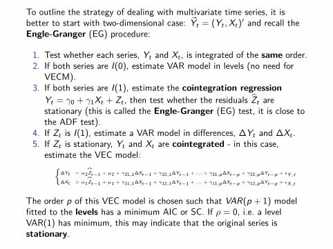
To outline the strategy of dealing with multivariate time series, it isbetter to start with two-dimensional case: ~Yt = (Yt ,Xt)′ and recall theEngle-Granger (EG) procedure:

1. Test whether each series, Yt and Xt , is integrated of the same order.2. If both series are I(0), estimate VAR model in levels (no need for

VECM).3. If both series are I(1), estimate the cointegration regression

Yt = γ0 + γ1Xt + Zt , then test whether the residuals Zt arestationary (this is called the Engle-Granger (EG) test, it is close tothe ADF test).

4. If Zt is I(1), estimate a VAR model in differences, ∆Yt and ∆Xt .5. If Zt is stationary, Yt and Xt are cointegrated - in this case,

estimate the VEC model:{∆Yt = α2 Zt−1 + µ2 + γ21,1∆Xt−1 + γ22,1∆Yt−1 + ... + γ21,p ∆Xt−p + γ22,p ∆Yt−p + εY ,t∆Xt = α1 Zt−1 + µ1 + γ11,1∆Xt−1 + γ12,1∆Yt−1 + ... + γ11,p ∆Xt−p + γ12,p ∆Yt−p + εX,t

The order p of this VEC model is chosen such that VAR(p + 1) modelfitted to the levels has a minimum AIC or SC. If ρ = 0, i.e. a levelVAR(1) has minimum, this may indicate that the original series isstationary.

6. If necessary, use the model obtained to forecast Yt and Xt (this canbe done by rewriting the VEC model as a VAR model). For example,the model:

∆~Yt = αβT ~Yt−1 + Γ1∆~Yt−1 + ~εt

can be expressed as a VAR(2):

~Yt = (I + Γ1 + αβT )~Yt−1 − Γ1~Yt−2 + ~εt

I Thus, in the case where our data consists of two I(1) components,we use the EG test for cointegration.

I In a multidimensional case we use another cointegration test calledthe Johansen test.

The first thing to note is that it is possible for more than onecointegrating relationship to exist if you are working with several timeseries variables (all of which you have tested and found to have unitroots). To be precise, if you are working with d variables, then it ispossible to have up to d − 1 cointegrating relationships (and, thus, up tod − 1 cointegrating residuals included in the VECM).

To begin with, let us return to equation:

∆~Yt = ~µt + αβT ~Yt−1 + Γ1∆~Yt−1 + ...+ Γt−p∆~Yt−p+1 + ~εt

I If rank(β) = 0, then only βT ~Yt−1 = 0 · Y1,t−1 + ...+ 0 · Yd,t−1 = 0is stationary. In other words, ~Yt is not cointegrated and VECMreduces to VAR(p − 1) in differences.

I If 0 < rank(β) = r < d , ~Yt is I(1) with r linearly independentcointegrating vectors and βt ~Yt−1 ∼ I(0).

I If rank(β) = d , then Π has full rank and is invertible, therefore ~Yt−1will be a linear combination of stationary differences, therefore,stationary itself.

Thus, it is often of interest to test, not simply for whether cointegratingis present or not, but also for the number of cointegratingrelationships. Recall that any hypothesis is rejected if the test statisticsexceeds the critical value. However, these critical values depend on thedeterministic components of VECM such as constants and linear trends.

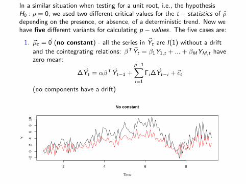
In a similar situation when testing for a unit root, i.e., the hypothesisH0 : ρ = 0, we used two different critical values for the t − statistics of ρdepending on the presence, or absence, of a deterministic trend. Now wehave five different variants for calculating p − values. The five cases are:

1. ~µt = ~0 (no constant) - all the series in ~Yt are I(1) without a driftand the cointegrating relations: βT ~Yt = β1Y1,t + ...+ βMYM,t havezero mean:

∆~Yt = αβT ~Yt−1 +p−1∑i=1

Γi ∆~Yt−i + ~εt

(no components have a drift)

No constant

Time

Y

2 4 6 8

−2

02

46

810

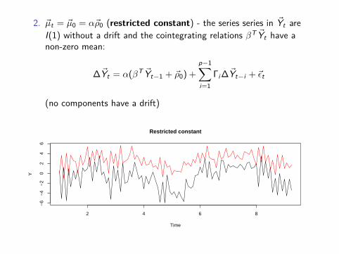
2. ~µt = ~µ0 = α~ρ0 (restricted constant) - the series series in ~Yt areI(1) without a drift and the cointegrating relations βT ~Yt have anon-zero mean:

∆~Yt = α(βT ~Yt−1 + ~ρ0) +p−1∑i=1

Γi ∆~Yt−i + ~εt

(no components have a drift)

Restricted constant

Time

Y

2 4 6 8

−6

−4

−2

02

46

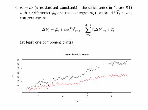
3. ~µt = ~µ0 (unrestricted constant) - the series series in ~Yt are I(1)with a drift vector ~µ0 and the cointegrating relations βT ~Yt have anon-zero mean:

∆~Yt = ~µ0 + αβT ~Yt−1 +p−1∑i=1

Γi ∆~Yt−i + ~εt

(at least one component drifts)

Unrestricted. constant

Time

Y

2 4 6 8

05

1015

2025

3035

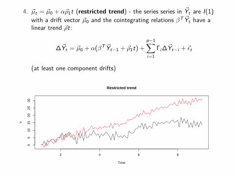
4. ~µt = ~µ0 + α~ρ1t (restricted trend) - the series series in ~Yt are I(1)with a drift vector ~µ0 and the cointegrating relations βT ~Yt have alinear trend ~ρt:

∆~Yt = ~µ0 + α(βT ~Yt−1 + ~ρ1t) +p−1∑i=1

Γi ∆~Yt−i + ~εt

(at least one component drifts)

Restricted trend

Time

Y

2 4 6 8

05

1015

2025

30

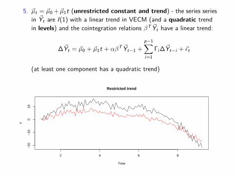
5. ~µt = ~µ0 + ~µ1t (unrestricted constant and trend) - the series seriesin ~Yt are I(1) with a linear trend in VECM (and a quadratic trendin levels) and the cointegration relations βT ~Yt have a linear trend:

∆~Yt = ~µ0 + ~µ1t + αβT ~Yt−1 +p−1∑i=1

Γi ∆~Yt−i + ~εt

(at least one component has a quadratic trend)

Restricted trend

Time

Y

2 4 6 8

−20

−10

010

Note: if no components of ~Yt drift - we use Cases 1 or 2. If at least onecomponent of ~Yt drifts - we use Case or 4. If at least one component of~Yt has a quadratic trend - we use Case 5.

I Case 1 is not really relevant for empirical work.I The restricted constant Case 2 is appropriate for non-trending I(1)

data like interest rates and exchange rates.I The unrestricted constant Case 3 is appropriate for trending I(1)

data like asset prices, macroeconomic aggregates (real GDP,consumption, employment etc).

I The restricted trend case 4 is also appropriate for trending I(1) as inCase 3. However, notice the deterministic trend in the cointegratingresidual in Case 4 as opposed to the stationary residuals in Case 3.

I The unrestricted trend Case 5 is appropriate for I(1) data with aquadratic trend. An example might be nominal price data duringtimes of extreme inflation.

The above-given figures and considerations are important in choosing theright variant to define critical values of the Johansen test. The basicsteps in Johansen’s methodology are (we assume that all the series in ~Ytare I(1)):

1. Choose the right order p for a VAR(p) model for levels.2. Choose the right case out of five ones (use graphs of ~Yt).3. Apply Johansen’s test and find the number of cointegrating relations.4. Create a VECM5. Use it to forecast ~Yt .

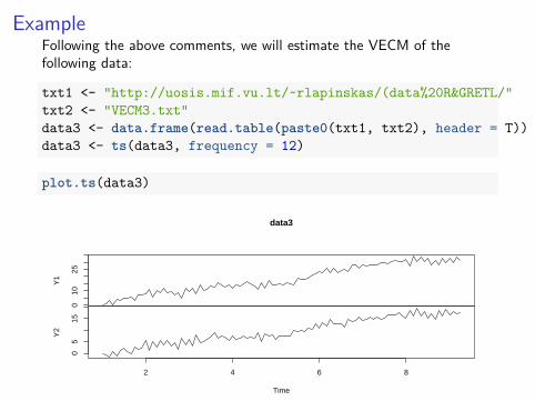
ExampleFollowing the above comments, we will estimate the VECM of thefollowing data:

txt1 <- "http://uosis.mif.vu.lt/~rlapinskas/(data%20R&GRETL/"txt2 <- "VECM3.txt"data3 <- data.frame(read.table(paste0(txt1, txt2), header = T))data3 <- ts(data3, frequency = 12)

plot.ts(data3)

010

25

Y1

05

15

2 4 6 8

Y2

Time

data3

0. Test for a unit root

mdl1 <- dynlm::dynlm(d(Y1) ~ L(Y1) + L(d(Y1), 1) + time(Y1),data = data3)

round(summary(mdl1)$coeff, 4)

## Estimate Std. Error t value Pr(>|t|)## (Intercept) 0.2282 0.4782 0.4772 0.6343## L(Y1) -0.2598 0.0962 -2.6996 0.0082## L(d(Y1), 1) -0.6426 0.0797 -8.0619 0.0000## time(Y1) 0.9663 0.3828 2.5239 0.0133

t-statistic = -2.6996 > 3.45 so we do not reject the nullhypothesis H0 : the process has a unit root .

mdl2 <- dynlm::dynlm(d(Y2) ~ L(Y2) + L(d(Y2), 1) + time(Y2),data = data3)

round(summary(mdl2)$coeff, 4)

## Estimate Std. Error t value Pr(>|t|)## (Intercept) -0.6287 0.4360 -1.4418 0.1527## L(Y2) -0.4141 0.1205 -3.4374 0.0009## L(d(Y2), 1) -0.5792 0.0852 -6.7950 0.0000## time(Y2) 0.9290 0.2823 3.2906 0.0014

t-statistic = -3.4374 > 3.45 so we do not reject the nullhypothesis H0 : the process has a unit root .

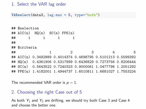
1. Select the VAR lag order

VARselect(data3, lag.max = 5, type="both")

## $selection## AIC(n) HQ(n) SC(n) FPE(n)## 1 1 1 1#### $criteria## 1 2 3 4 5## AIC(n) 0.3492889 0.4014374 0.4698795 0.5101213 0.5599392## HQ(n) 0.4361906 0.5317899 0.6436829 0.7273756 0.8206444## SC(n) 0.5643522 0.7240323 0.9000061 1.0477796 1.2051292## FPE(n) 1.4182001 1.4944737 1.6010811 1.6681027 1.7553224

The recommended VAR order is p = 1.

2. Choosing the right Case out of 5As both Y1 and Y2 are drifting, we should try both Case 3 and Case 4and choose the better one.

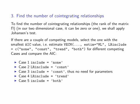
3. Find the number of cointegrating relationshipsTo find the number of cointegrating relationships (the rank of the matrixΠ) (in our two dimensional case, it can be zero or one), we shall applyJohansen’s test.

If there are a couple of competing models, select the one with thesmallest AIC value, i.e. estimate VECM(..., estim="ML", LRinclude= c("none", "const", "trend", "both") for different competingCases and compare the AIC:

I Case 1 include = 'none'I Case 2 LRinclude = 'const'I Case 3 include = 'const', thus no need for parametersI Case 4 LRinclude = 'trend'I Case 5 include = 'both'

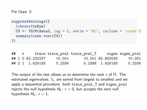
For Case 3:

suppressWarnings({library(tsDyn)C3 <- VECM(data3, lag = 1, estim = "ML", include = 'const')summary(rank.test(C3))

})

## r trace trace_pval trace_pval_T eigen eigen_pval## 1 0 62.222227 <0.001 <0.001 60.802033 <0.001## 2 1 1.420193 0.2334 0.2398 1.420193 0.2334

The output of the test allows us to determine the rank r of Π. Theestimated eigenvalues, λi , are sorted from largest to smallest and weapply a sequential procedure: both trace_pval_T and eigen_pvalrejects the null hypothesis H0 : r = 0, but accepts the next nullhypothesis H0 : r = 1.

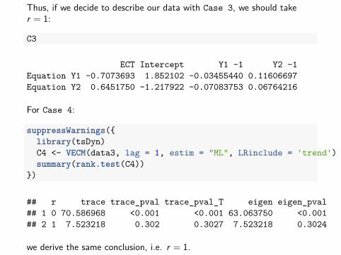
Thus, if we decide to describe our data with Case 3, we should taker = 1:

C3

ECT Intercept Y1 -1 Y2 -1Equation Y1 -0.7073693 1.852102 -0.03455440 0.11606697Equation Y2 0.6451750 -1.217922 -0.07083753 0.06764216

For Case 4:

suppressWarnings({library(tsDyn)C4 <- VECM(data3, lag = 1, estim = "ML", LRinclude = 'trend')summary(rank.test(C4))

})

## r trace trace_pval trace_pval_T eigen eigen_pval## 1 0 70.586968 <0.001 <0.001 63.063750 <0.001## 2 1 7.523218 0.302 0.3027 7.523218 0.3024

we derive the same conclusion, i.e. r = 1.

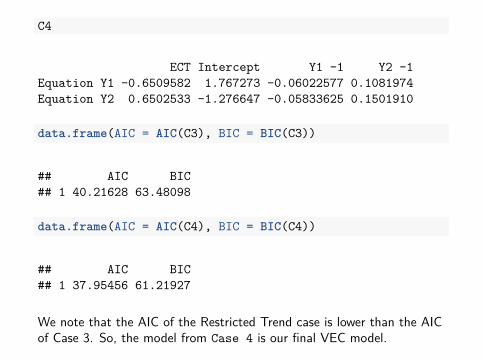
C4

ECT Intercept Y1 -1 Y2 -1Equation Y1 -0.6509582 1.767273 -0.06022577 0.1081974Equation Y2 0.6502533 -1.276647 -0.05833625 0.1501910

data.frame(AIC = AIC(C3), BIC = BIC(C3))

## AIC BIC## 1 40.21628 63.48098

data.frame(AIC = AIC(C4), BIC = BIC(C4))

## AIC BIC## 1 37.95456 61.21927

We note that the AIC of the Restricted Trend case is lower than the AICof Case 3. So, the model from Case 4 is our final VEC model.

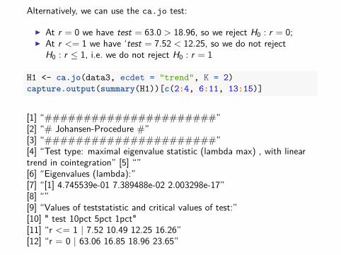
Alternatively, we can use the ca.jo test:

I At r = 0 we have test = 63.0 > 18.96, so we reject H0 : r = 0;I At r <= 1 we have ‘test = 7.52 < 12.25, so we do not reject

H0 : r ≤ 1, i.e. we do not reject H0 : r = 1

H1 <- ca.jo(data3, ecdet = "trend", K = 2)capture.output(summary(H1))[c(2:4, 6:11, 13:15)]

[1] “######################”[2] “# Johansen-Procedure #”[3] “######################”[4] “Test type: maximal eigenvalue statistic (lambda max) , with lineartrend in cointegration” [5] “”[6] “Eigenvalues (lambda):”[7] “[1] 4.745539e-01 7.389488e-02 2.003298e-17”[8] “”[9] “Values of teststatistic and critical values of test:”[10] " test 10pct 5pct 1pct"[11] “r <= 1 | 7.52 10.49 12.25 16.26”[12] “r = 0 | 63.06 16.85 18.96 23.65”

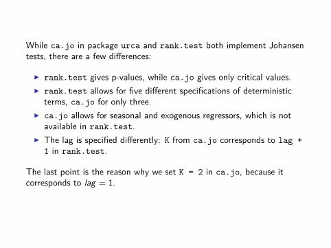
While ca.jo in package urca and rank.test both implement Johansentests, there are a few differences:

I rank.test gives p-values, while ca.jo gives only critical values.I rank.test allows for five different specifications of deterministic

terms, ca.jo for only three.I ca.jo allows for seasonal and exogenous regressors, which is not

available in rank.test.I The lag is specified differently: K from ca.jo corresponds to lag +

1 in rank.test.

The last point is the reason why we set K = 2 in ca.jo, because itcorresponds to lag = 1.

4. Create a VECM

C4$coefficients

## ECT Intercept Y1 -1 Y2 -1## Equation Y1 -0.6509582 1.767273 -0.06022577 0.1081974## Equation Y2 0.6502533 -1.276647 -0.05833625 0.1501910

t(C4$model.specific$beta)

## Y1 Y2 trend## r1 1 -1.883276 0.03712441

{∆Y1,t = 1.767 − 0.65 · (Y1,t−1 − 1.88Y2,t−1 + 0.0371(t − 1))∆Y2,t = −1.277 + 0.65 · (Y2,t−1 − 1.88Y2,t−1 + 0.0371(t − 1))

Coefficient (α =) ECT = 0.65 is called an adjustment coefficient. Itindicates that Y2 will return to equilibrium in 1/0.65 ∼ 2 steps, ceterisparibus.

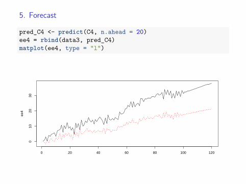
5. Forecast

pred_C4 <- predict(C4, n.ahead = 20)ee4 = rbind(data3, pred_C4)matplot(ee4, type = "l")

0 20 40 60 80 100 120

010

2030

ee4

Remarks

I If we have two variables, both Engle-Granger and Johansen tests areappropriate for cointegration.In a multidimensional case, the EGsuffers from omitted variable bias, so in those cases it is better touse Johansen test.

I The most restricted model (Case 1) is unlikely to find general use,because at least a constant will usually be included in thecointegration equation.

I The least restricted model (Case 5) allows for quadratic trends inthe data which occurs quite rarely.

I The choice between Case 2 and Case 3 rests upon whether there isa need to allow for the possibility of linear trends in the data, apreliminary graphing of the data is often helpful in this respect.

I If Case 3 is preferred to Case 2, only then does Case 4 need to beconsidered since the data has to have a linear trend if we are toconsider allowing a trend in the cointegration equation.

I As a rough guide, use Case 2 if none of the series appear to have atrend.

I For trending series, use Case 3 if you believe all trends arestochastic.

I If you believe some of the series are trend stationary, use Case 4.

However, the simplest way that also allows one to “automate” selectionis to choose the case according to the minimum of AIC of BIC of themodel.

Multivariate VAR is a complicated model. Below we present some usefulfacts without proofs:

I To estimate the coefficients of~Yt = ~α + ~δt + Θ1~Yt−1 + ...+ Θp ~Yt−p + ~εt use the (conditional)maximum likelihood estimation method, assuming tat theinnovations ~εt have a multivariate normal distribution. This isequivalent to OLS method applied to each equation separately.

I Maximum likelihood estimates are consistent even if the trueinnovations are non-Gaussian.

I Standard OLS t and F statistics applied to the coefficients of anysingle equation of the VAR are asymptotically valid.

I The goal of unit root tests is to find a parsimonious representationof the data that gives a reasonable approximation of the trueprocess, as opposed to determining whether or not the true processis literally I(1).

I If ~Yt is cointegrated, a VAR estimated in levels is not misspecifiedbut involves a loss of efficiency.

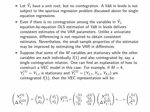
I Let ~Yt have a unit root, but no cointegration. A VAR in levels is notsubject to the spurious regression problem discussed above for singleequation regressions.

I Even if there is no cointegration among the variables in ~Yt ,equation-by-equation OLS estimation of VAR in levels deliversconsistent estimates of the VAR parameters. Unlike a univariateregression, differencing is not required to obtain consistentestimates. Nevertheless, the small sample properties of the estimatormay be improved by estimating the VAR in differences.

I Suppose that some of the M variables are stationary while the othervariables are each individually I(1) and also cointegrated by, say, asingle cointegration relation. One can find an explanation of how toconstruct a VEC model in this case. For example, if M = 4,Y (1)

t = Y1,t is stationary and ~Y (2)t = (Y2,t ,Y3,t ,Y4,t) are

cointegrated I(1), then the VEC representation will be:

(Y (1)

t∆~Y (2)

t

)=(µ1~µ2

)+(~π1~π2

)~Y (2)

t−1 +(γ

(1)11 ~γ

(1)12

γ(1)21 ~γ

(1)22

)(Y (1)

t−1∆~Y (2)

t−1

)+ ...+

(ε

(1)t~ε

(2)t

)