統計模型與 迴歸分析 本章大綱與學習目標 統計模型配適...
TRANSCRIPT

http://www.hmwu.idv.tw http://www.hmwu.idv.tw
吳漢銘國立臺北大學 統計學系
統計模型與迴歸分析
B05
http://www.hmwu.idv.tw
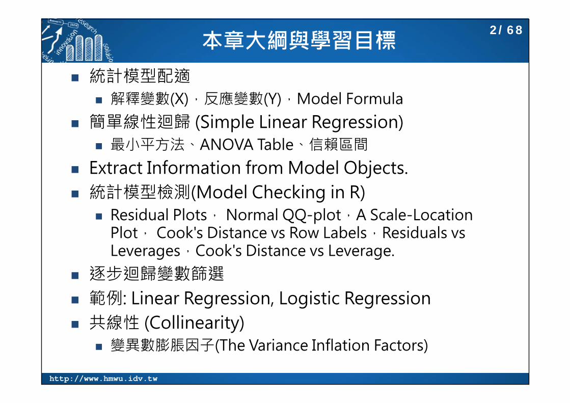
本章大綱與學習目標 統計模型配適
解釋變數(X),反應變數(Y),Model Formula
簡單線性迴歸 (Simple Linear Regression) 最小平方法、ANOVA Table、信賴區間
Extract Information from Model Objects. 統計模型檢測(Model Checking in R)
Residual Plots, Normal QQ-plot,A Scale-Location Plot, Cook's Distance vs Row Labels,Residuals vs Leverages,Cook's Distance vs Leverage.
逐步迴歸變數篩選 範例: Linear Regression, Logistic Regression 共線性 (Collinearity)
變異數膨脹因子(The Variance Inflation Factors)
2/68

http://www.hmwu.idv.tw
統計模型配適 (Statistical Modeling)四個問題:1. Which of your variables is the response variable (反應變數, Y)?
2. Which are the explanatory variable (解釋變數, X)?
3. Are the explanatory variables continuous (連續) or categorical (類別), or a mixture (混合) of both?
4. What kind of response variable do you have: continuousmeasurement, a count, a proportion, a time at death, or category?
配適統計模型的目的 To determine the values of the parameters in a specific model that
lead to the best fit of the model to the data.
3/68

http://www.hmwu.idv.tw
解釋變數, X
The Explanatory Variable (X) All x's are continuous: Regression
All x's are categorical: Analysis of Variance (ANOVA, 變異數分析)
x's are both continuous and categorical: Analysis of Covariance (ANCOVA)
例如:
例如:
例如:
4/68
http://www.hmwu.idv.tw
反應變數, Y (1)
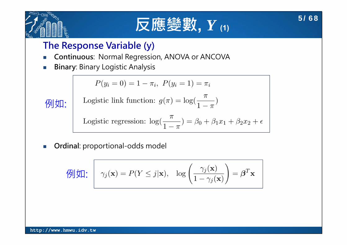
The Response Variable (y) Continuous: Normal Regression, ANOVA or ANCOVA Binary: Binary Logistic Analysis
Ordinal: proportional-odds model
例如:
例如:
5/68

http://www.hmwu.idv.tw
反應變數, Y (2)
Count: Log-Linear Models
Time at death: Survival Analysis
例如:
6/68

http://www.hmwu.idv.tw
模式寫法 (Model Formulae in R) The structure of the model: response.variable ~ explanatory.variables
Example: fm <- formula(y ~ x) Example: lm(fm), lm(y ~ x); aov(y ~ x); glm(y ~ x)
~: "is modelled as a function of" Example: lm(y ~ x)
+ : inclusion of an explanatory variable in the model (not addition); Example: lm(y ~ x1 + x2)
- : deletion of an explanatory variable from the model (not subtraction); Example: lm(y ~ x1 - 1)
* : inclusion of explanatory variables and interactions (not multiplication); Example: lm(y ~ x1 * x2)
/: nesting of explanatory variables in the model (not division); Example: lm(y ~ x1 / x2) # x1因子的各分類下,再細分出x2因子的分類
7/68
http://www.hmwu.idv.tw
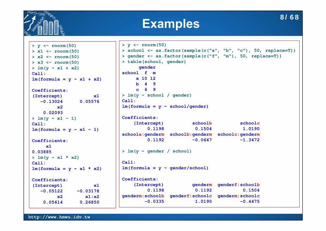
Examples> y <- rnorm(50)> x1 <- rnorm(50)> x2 <- rnorm(50)> x3 <- rnorm(50)> lm(y ~ x1 + x2)Call:lm(formula = y ~ x1 + x2)
Coefficients:(Intercept) x1
-0.13024 0.05576x2
0.02093> lm(y ~ x1 - 1)Call:lm(formula = y ~ x1 - 1)
Coefficients:x1
0.03885 > lm(y ~ x1 * x2)Call:lm(formula = y ~ x1 * x2)
Coefficients:(Intercept) x1
-0.05122 -0.03178x2 x1:x2
0.05614 0.26850
> y <- rnorm(50)> school <- as.factor(sample(c("a", "b", "c"), 50, replace=T))> gender <- as.factor(sample(c("f", "m"), 50, replace=T))> table(school, gender)
genderschool f m
a 10 12b 4 9c 6 9
> lm(y ~ school / gender)Call:lm(formula = y ~ school/gender)
Coefficients:(Intercept) schoolb schoolc
0.1198 0.1504 1.0190 schoola:genderm schoolb:genderm schoolc:genderm
0.1192 -0.0647 -1.3472
> lm(y ~ gender / school)
Call:lm(formula = y ~ gender/school)
Coefficients:(Intercept) genderm genderf:schoolb
0.1198 0.1192 0.1504 genderm:schoolb genderf:schoolc genderm:schoolc
-0.0335 1.0190 -0.4475
8/68

http://www.hmwu.idv.tw
模式寫法 (Model Formulae in R) |: indicates conditioning (not ‘or’), so that y ~ x | z is read as ‘y
as a function of x given z". Example: lm(y ~ x1 | x2)
":" : a colon denotes an interaction A:B means the two-way interaction between A and B N:P:K:Mg means the four-way interaction between N, P, K and Mg.
> lm(y ~ x1 | x2)
Call:lm(formula = y ~ x1 | x2)
Coefficients:(Intercept) x1 | x2TRUE
-0.1216 NA
> lm(y ~ x1:x2:x3)
Call:lm(formula = y ~ x1:x2:x3)
Coefficients:(Intercept) x1:x2:x3
-0.08602 -0.20145
> ##Create a formula for a model with a large number of variables:> xnam <- paste("x", 1:25, sep="")> (fmla <- as.formula(paste("y ~ ", paste(xnam, collapse= "+"))))y ~ x1 + x2 + x3 + x4 + x5 + x6 + x7 + x8 + x9 + x10 + x11 +
x12 + x13 + x14 + x15 + x16 + x17 + x18 + x19 + x20 + x21 + x22 + x23 + x24 + x25
9/68

http://www.hmwu.idv.tw
模式寫法 (Model Formulae in R) A*B*C is the same as A+B+C+A:B+A:C+B:C+A:B:C A/B/C is the same as A+B%in%A+C%in%B%in%A (A+B+C)^3 is the same as A*B*C (A+B+C)^2 is the same as A*B*C – A:B:C
> lm(y ~ A*B*C)
Call:lm(formula = y ~ A * B * C)
Coefficients:(Intercept) A B
0.20776 -0.04336 0.01105 C A:B A:C
-0.06969 0.14857 -0.02269 B:C A:B:C
-0.06689 0.08850
> lm(y ~ A/B/C)
Call:lm(formula = y ~ A/B/C)
Coefficients:(Intercept) A A:B
0.21586 -0.06219 0.12840 A:B:C
0.07229
> y <- rnorm(50)> A <- rnorm(50)> B <- rnorm(50)> C <- rnorm(50)
> lm(y ~ (A+B+C)^3)
Call:lm(formula = y ~ (A + B + C)^3)
Coefficients:(Intercept) A B C
0.20776 -0.04336 0.01105 -0.06969 A:B A:C B:C A:B:C
0.14857 -0.02269 -0.06689 0.08850
> lm(y ~ (A+B+C)^2)
Call:lm(formula = y ~ (A + B + C)^2)
Coefficients:(Intercept) A B C
0.21990 -0.03953 0.02210 -0.05622 A:B A:C B:C
0.15181 -0.05379 -0.03787
10/68
http://www.hmwu.idv.tw
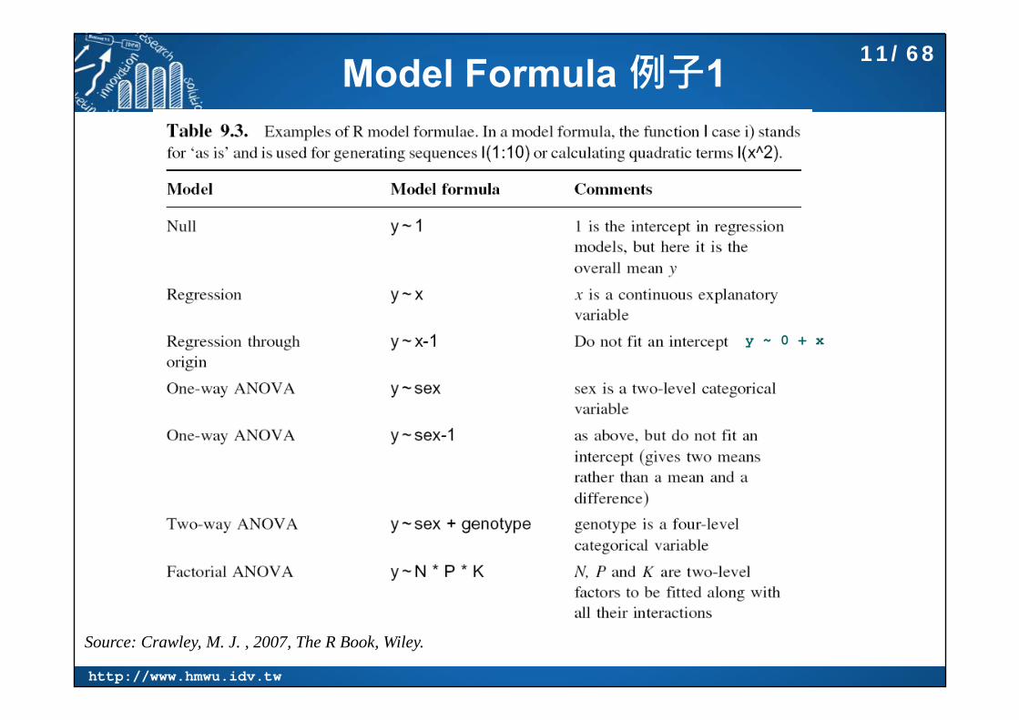
Model Formula 例子1
Source: Crawley, M. J. , 2007, The R Book, Wiley.
y ~ 0 + x
11/68

http://www.hmwu.idv.tw
Model Formula 例子2
Source: Crawley, M. J. , 2007, The R Book, Wiley.
12/68

http://www.hmwu.idv.tw
Model Formula 例子 3
Source: Crawley, M. J. , 2007, The R Book, Wiley.
13/68

http://www.hmwu.idv.tw
Statistical Models in R
Source: Crawley, M. J. , 2007, The R Book, Wiley.
14/68

http://www.hmwu.idv.tw
簡單線性迴歸 (Simple Linear Regression)
beta_0 (intercept), beta_1 (slope): parameters to be estimated from observed data. Random errors (epsilon): mean zero and unknown variance (sigma^2). The variance in y is constant (i.e. the variance does not change as y gets bigger).
> wind <- airquality$Wind> temp <- airquality$Temp> plot(temp, wind, main="scatterplot of wind vs temp")
15/68

http://www.hmwu.idv.tw
參數估計: 最小平方法> y <- airquality$Wind> x <- airquality$Temp> xbar <- mean(x) ; xbar[1] 77.88235> ybar <- mean(y) ; ybar[1] 9.957516
> beta1.num <- sum((x-xbar)*(y-ybar))> beta1.den <- sum((x-xbar)^2)> (beta1.hat <- beta1.num/beta1.den)[1] -0.1704644
> (beta0.hat <- ybar-beta1.hat*xbar) [1] 23.23369> yhat <- beta0.hat + beta1.hat * x
> Sxy <- sum(y*(x-xbar)) ; Sxy[1] -2321.365> Sxx <- sum((x-xbar)^2) ; Sxx[1] 13617.88> Syy <- sum((y-ybar)^2) ; Syy[1] 1886.554> beta1.hat2 <- Sxy/Sxx ; beta1.hat2[1] -0.1704644
16/68

http://www.hmwu.idv.tw
最小平方法
> wind <- airquality$Wind> temp <- airquality$Temp
> n <- length(wind)> index <- sample(1:n, 10)> wind.subset <- wind[index]> temp.subset <- temp[index]
> plot(wind.subset~temp.subset, main="subset of wind vs temp")> subset.lm <- lm(wind.subset~temp.subset)> abline(subset.lm, col="red")> segments(temp.subset, fitted(subset.lm), temp.subset, wind.subset)
和 summary(lm(y~x))比較
17/68

http://www.hmwu.idv.tw
Find the Least Squares Fit> model.fit <- lsfit(temp, wind)> ls.print(model.fit)Residual Standard Error=3.1422R-Square=0.2098F-statistic (df=1, 151)=40.0795p-value=0
Estimate Std.Err t-value Pr(>|t|)Intercept 23.2337 2.1124 10.9987 0X -0.1705 0.0269 -6.3308 0
> plot(temp, wind, main="temp vs wind", pch=20)> abline(model.fit, col="red")> text(80,19, "Regression line:")> text(80,18, "y = 23.2337 - 0.1705 x")
18/68
http://www.hmwu.idv.tw
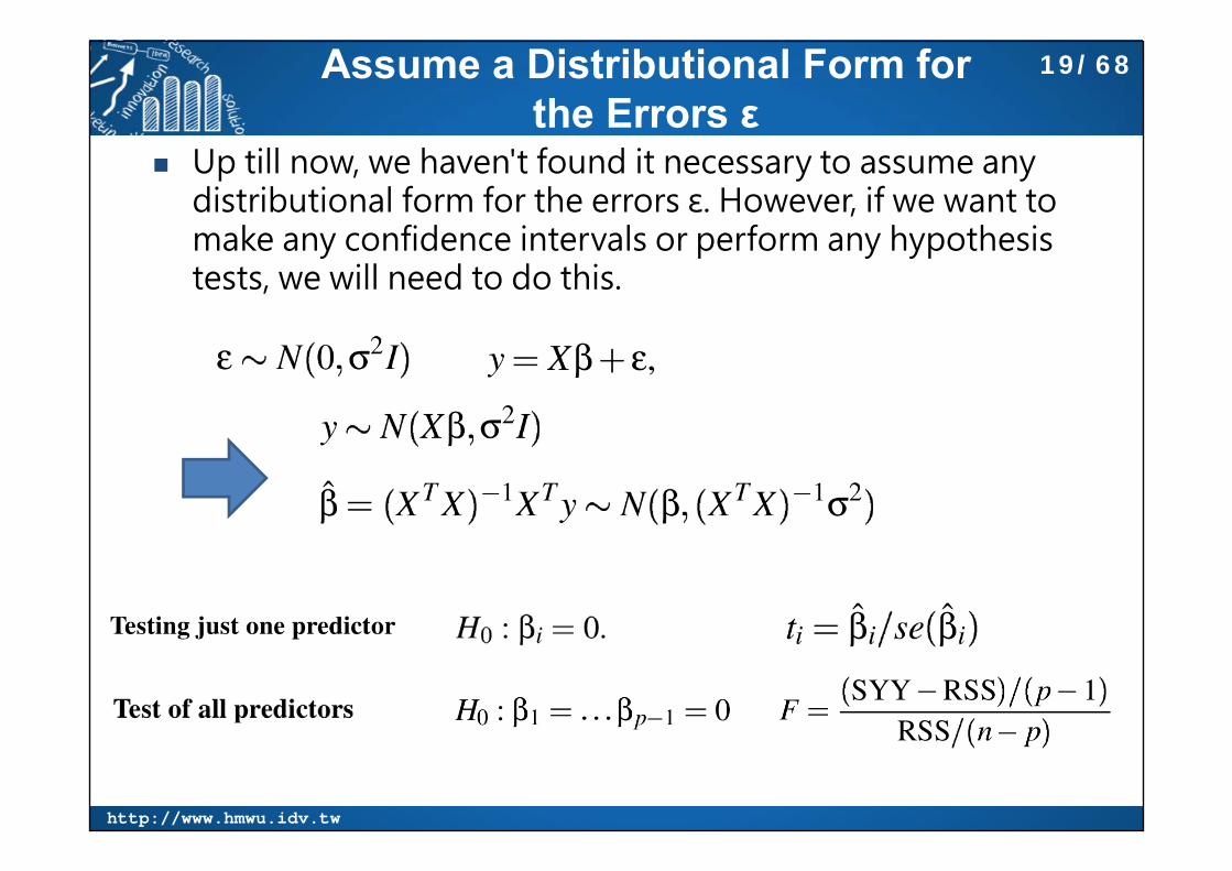
Assume a Distributional Form for the Errors ε
Up till now, we haven't found it necessary to assume any distributional form for the errors ε. However, if we want to make any confidence intervals or perform any hypothesis tests, we will need to do this.
19/68
http://www.hmwu.idv.tw
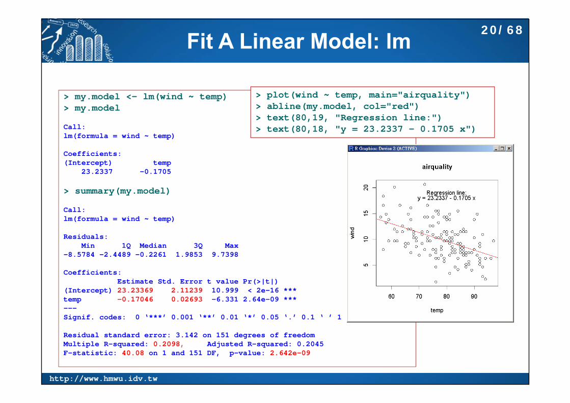
Fit A Linear Model: lm
> my.model <- lm(wind ~ temp)> my.model
Call:lm(formula = wind ~ temp)
Coefficients:(Intercept) temp
23.2337 -0.1705
> summary(my.model)
Call:lm(formula = wind ~ temp)
Residuals:Min 1Q Median 3Q Max
-8.5784 -2.4489 -0.2261 1.9853 9.7398
Coefficients:Estimate Std. Error t value Pr(>|t|)
(Intercept) 23.23369 2.11239 10.999 < 2e-16 ***temp -0.17046 0.02693 -6.331 2.64e-09 ***---Signif. codes: 0 ‘***’ 0.001 ‘**’ 0.01 ‘*’ 0.05 ‘.’ 0.1 ‘ ’ 1
Residual standard error: 3.142 on 151 degrees of freedomMultiple R-squared: 0.2098, Adjusted R-squared: 0.2045 F-statistic: 40.08 on 1 and 151 DF, p-value: 2.642e-09
> plot(wind ~ temp, main="airquality")> abline(my.model, col="red")> text(80,19, "Regression line:")> text(80,18, "y = 23.2337 - 0.1705 x")
20/68
http://www.hmwu.idv.tw
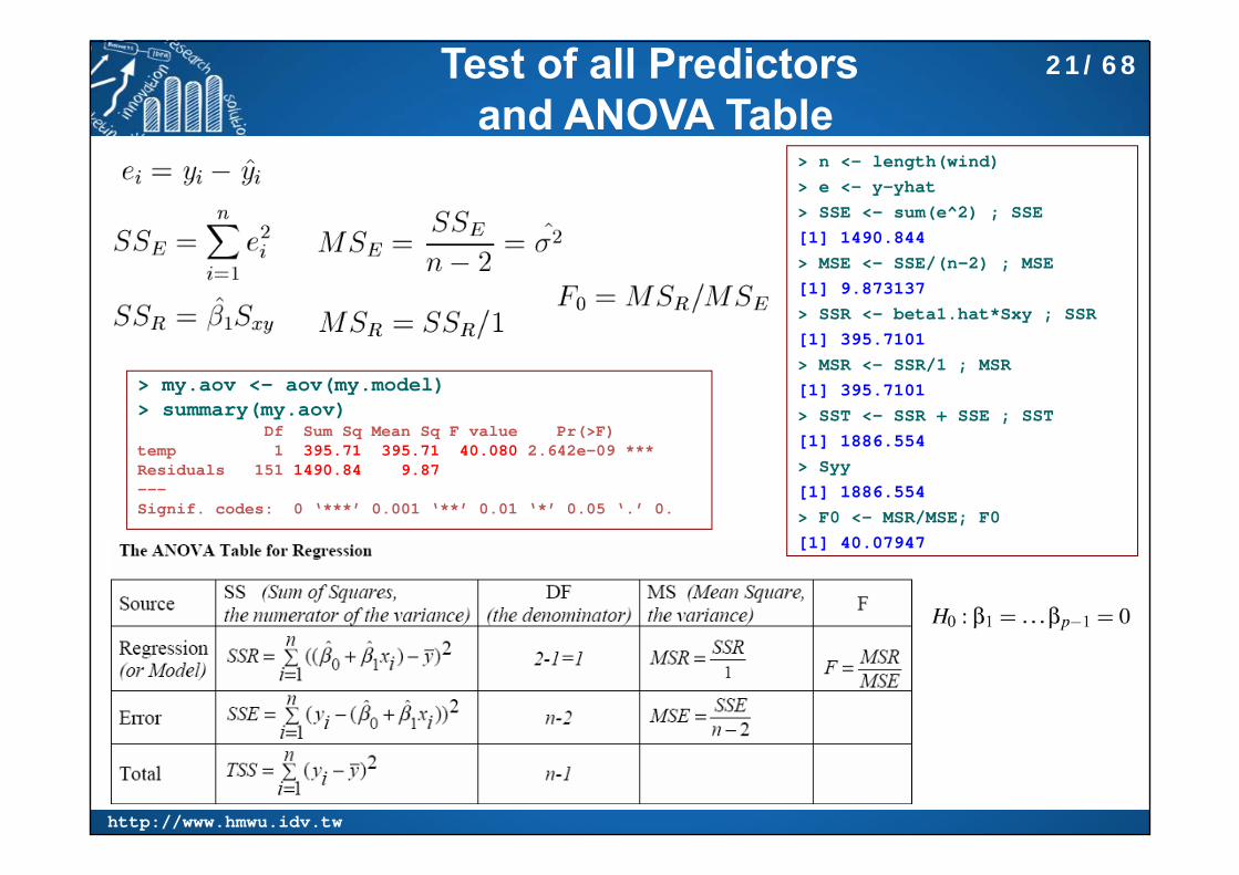
Test of all Predictorsand ANOVA Table
> n <- length(wind)> e <- y-yhat> SSE <- sum(e^2) ; SSE[1] 1490.844> MSE <- SSE/(n-2) ; MSE[1] 9.873137> SSR <- beta1.hat*Sxy ; SSR[1] 395.7101> MSR <- SSR/1 ; MSR[1] 395.7101> SST <- SSR + SSE ; SST[1] 1886.554> Syy[1] 1886.554> F0 <- MSR/MSE; F0[1] 40.07947
> my.aov <- aov(my.model)> summary(my.aov)
Df Sum Sq Mean Sq F value Pr(>F) temp 1 395.71 395.71 40.080 2.642e-09 ***Residuals 151 1490.84 9.87---Signif. codes: 0 ‘***’ 0.001 ‘**’ 0.01 ‘*’ 0.05 ‘.’ 0.
21/68

http://www.hmwu.idv.tw
課堂練習1: 估計量
用R寫出以下估計量,並與上述例子的答案比較。
決定系數 Coefficient of Determination
22/68

http://www.hmwu.idv.tw
參數估計之信賴區間
> alpha <- 0.05> se.beta0 <- sqrt(MSE*(1/n+xbar^2/Sxx)) ; se.beta0[1] 2.112395> tstar <- qt(alpha/2, n-1)* se.beta0 > CI.beta0 <- beta0.hat + c(-tstar*se.beta0, tstar*se.beta0) ; CI.beta0[1] 32.04965 14.41772
> se.beta1 <- sqrt(MSE/Sxx) ; se.beta1[1] 0.02692606> tstar <- qt(alpha/2, n-1)* se.beta1 > CI.beta1 <- beta1.hat + c(-tstar*se.beta0, tstar*se.beta1); CI.beta1[1] -0.0580900 -0.1718968
23/68
http://www.hmwu.idv.tw
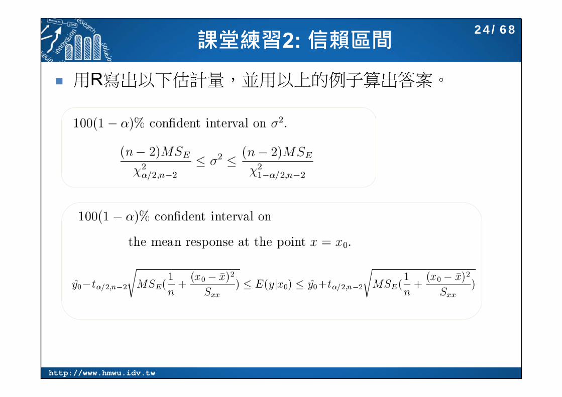
課堂練習2: 信賴區間
用R寫出以下估計量,並用以上的例子算出答案。
24/68

http://www.hmwu.idv.tw
Generic Functions
summary: produces parameter estimates and standard errors from lm, and ANOVA tables from aov.
plot: produces diagnostic plots for model checking, including residuals against fitted values, influence tests, etc.
update: is used to modify the last model fit; it saves both typing effort and computing time.
predict: uses information from the fitted model to produce smooth functions for plotting a line through the scatterplot of your data.
fitted: gives the fitted values, predicted by the model for the values of the explanatory variables included.
resid: gives the residuals.
> my.model <- lm(wind ~ temp)> summary(my.model)
25/68

http://www.hmwu.idv.tw
Extract Information from Model Objects
方法一: by functions> my.model <- lm(wind ~ temp)> summary(my.model)
Call:lm(formula = wind ~ temp)
Residuals:Min 1Q Median 3Q Max
-8.5784 -2.4489 -0.2261 1.9853 9.7398
Coefficients:Estimate Std. Error t value Pr(>|t|)
(Intercept) 23.23369 2.11239 10.999 < 2e-16 ***temp -0.17046 0.02693 -6.331 2.64e-09 ***---Signif. codes: 0 ‘***’ 0.001 ‘**’ 0.01 ‘*’ 0.05 ‘.’ 0.1 ‘ ’ 1
Residual standard error: 3.142 on 151 degrees of freedomMultiple R-squared: 0.2098, Adjusted R-squared: 0.2045 F-statistic: 40.08 on 1 and 151 DF, p-value: 2.642e-09
> coef(my.model)(Intercept) temp 23.2336881 -0.1704644
> vcov(my.model)(Intercept) temp
(Intercept) 4.46221130 -0.0564656925temp -0.05646569 0.0007250127
26/68
http://www.hmwu.idv.tw
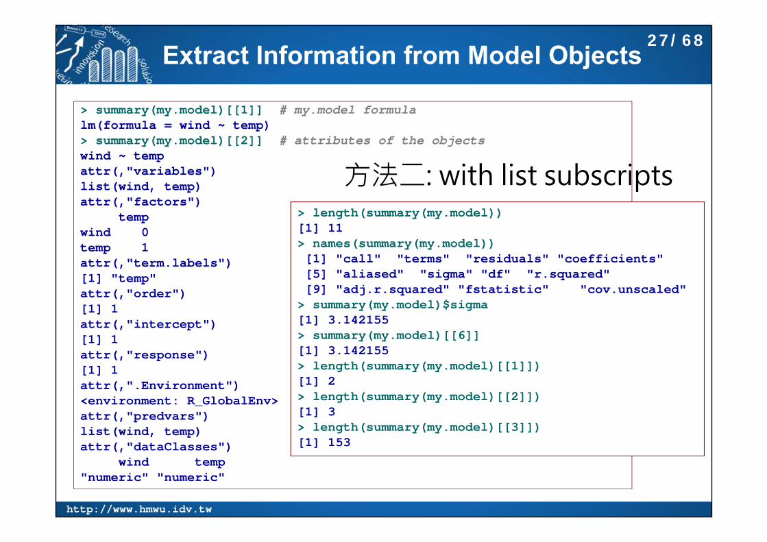
Extract Information from Model Objects
> summary(my.model)[[1]] # my.model formulalm(formula = wind ~ temp)> summary(my.model)[[2]] # attributes of the objectswind ~ tempattr(,"variables")list(wind, temp)attr(,"factors")
tempwind 0temp 1attr(,"term.labels")[1] "temp"attr(,"order")[1] 1attr(,"intercept")[1] 1attr(,"response")[1] 1attr(,".Environment")<environment: R_GlobalEnv>attr(,"predvars")list(wind, temp)attr(,"dataClasses")
wind temp "numeric" "numeric"
方法二: with list subscripts> length(summary(my.model))[1] 11> names(summary(my.model))[1] "call" "terms" "residuals" "coefficients" [5] "aliased" "sigma" "df" "r.squared" [9] "adj.r.squared" "fstatistic" "cov.unscaled"
> summary(my.model)$sigma[1] 3.142155> summary(my.model)[[6]][1] 3.142155> length(summary(my.model)[[1]])[1] 2> length(summary(my.model)[[2]])[1] 3> length(summary(my.model)[[3]])[1] 153
27/68

http://www.hmwu.idv.tw
Extract Information from Model Objects
方法二: with list subscripts> summary(my.model)[[3]] # residuals for data points
1 2 3 4 5 6 -4.41257055 -2.96024835 1.98068054 -1.16489276 0.61232059 2.91696501 ...145 146 147 148 149 150 -1.93071279 0.87393162 -1.17164167 4.10557168 -4.40117723 3.09207386
151 152 153 3.85114498 -2.27839058 -0.14210611
> summary(my.model)[[4]] # parameters tableEstimate Std. Error t value Pr(>|t|)
(Intercept) 23.2336881 2.11239468 10.998744 4.901351e-21temp -0.1704644 0.02692606 -6.330835 2.641597e-09
> summary(my.model)[[4]][[1]] # intercept[1] 23.23369
> summary(my.model)[[4]][[2]] # slope,.... summary(my.model)[[4]][[28]][1] -0.1704644
> str(summary(my.model)[[4]])num [1:2, 1:4] 23.2337 -0.1705 2.1124 0.0269 10.9987 ...- attr(*, "dimnames")=List of 2..$ : chr [1:2] "(Intercept)" "temp"..$ : chr [1:4] "Estimate" "Std. Error" "t value" "Pr(>|t|)"
28/68
http://www.hmwu.idv.tw
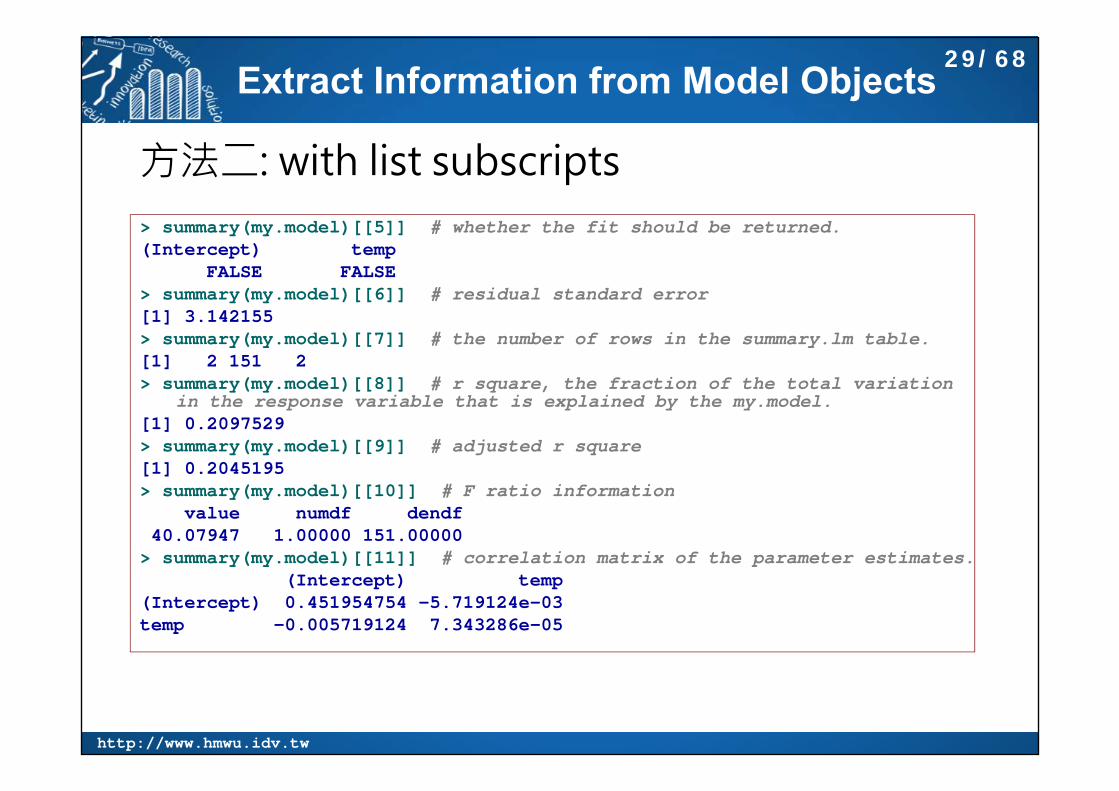
Extract Information from Model Objects
方法二: with list subscripts> summary(my.model)[[5]] # whether the fit should be returned.(Intercept) temp
FALSE FALSE> summary(my.model)[[6]] # residual standard error[1] 3.142155> summary(my.model)[[7]] # the number of rows in the summary.lm table.[1] 2 151 2> summary(my.model)[[8]] # r square, the fraction of the total variation
in the response variable that is explained by the my.model.[1] 0.2097529> summary(my.model)[[9]] # adjusted r square[1] 0.2045195> summary(my.model)[[10]] # F ratio information
value numdf dendf40.07947 1.00000 151.00000
> summary(my.model)[[11]] # correlation matrix of the parameter estimates.(Intercept) temp
(Intercept) 0.451954754 -5.719124e-03temp -0.005719124 7.343286e-05
29/68

http://www.hmwu.idv.tw
Extract Information from Model Objects
> my.model <- lm(wind ~ temp)> names(my.model)[1] "coefficients" "residuals" "effects" "rank" [5] "fitted.values" "assign" "qr" "df.residual" [9] "xlevels" "call" "terms" "model"
> model$coefficients> model$fitted.values> model$residuals
> summary.aov(my.model)> summary.aov(my.model)[[1]][[1]]~> summary.aov(my.model)[[1]][[5]]
方法三: using $
依此類推...
30/68
http://www.hmwu.idv.tw
Extract Information from Model Objects
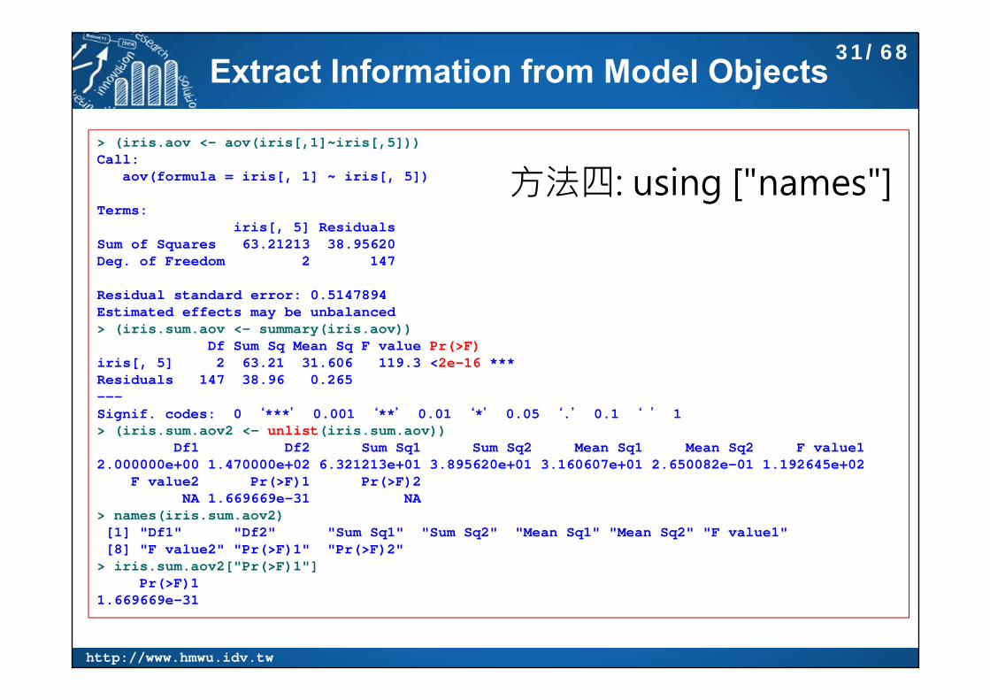
> (iris.aov <- aov(iris[,1]~iris[,5]))Call:
aov(formula = iris[, 1] ~ iris[, 5])
Terms:iris[, 5] Residuals
Sum of Squares 63.21213 38.95620Deg. of Freedom 2 147
Residual standard error: 0.5147894Estimated effects may be unbalanced> (iris.sum.aov <- summary(iris.aov))
Df Sum Sq Mean Sq F value Pr(>F) iris[, 5] 2 63.21 31.606 119.3 <2e-16 ***Residuals 147 38.96 0.265 ---Signif. codes: 0 ‘***’ 0.001 ‘**’ 0.01 ‘*’ 0.05 ‘.’ 0.1 ‘ ’ 1> (iris.sum.aov2 <- unlist(iris.sum.aov))
Df1 Df2 Sum Sq1 Sum Sq2 Mean Sq1 Mean Sq2 F value1 2.000000e+00 1.470000e+02 6.321213e+01 3.895620e+01 3.160607e+01 2.650082e-01 1.192645e+02
F value2 Pr(>F)1 Pr(>F)2 NA 1.669669e-31 NA
> names(iris.sum.aov2)[1] "Df1" "Df2" "Sum Sq1" "Sum Sq2" "Mean Sq1" "Mean Sq2" "F value1"[8] "F value2" "Pr(>F)1" "Pr(>F)2"
> iris.sum.aov2["Pr(>F)1"]Pr(>F)1
1.669669e-31
方法四: using ["names"]
31/68

http://www.hmwu.idv.tw
使用子集合做分析 Investigate how much a influence point affected the parameter estimates and their
standard error. Repeat the statistical modeling but leave out the point in question, using subset.
> new.model <- update(my.model, subset=(temp!=max(temp)))> summary(new.model)
Call:lm(formula = wind ~ temp, subset = (temp != max(temp)))
Residuals:Min 1Q Median 3Q Max
-8.5663 -2.3871 -0.2027 1.9662 9.7344
Coefficients:Estimate Std. Error t value Pr(>|t|)
(Intercept) 23.5529 2.1382 11.015 < 2e-16 ***temp -0.1748 0.0273 -6.403 1.85e-09 ***---Signif. codes: 0 ‘***’ 0.001 ‘**’ 0.01 ‘*’ 0.05 ‘.’ 0.1 ‘ ’ 1
Residual standard error: 3.143 on 150 degrees of freedomMultiple R-squared: 0.2147, Adjusted R-squared: 0.2094 F-statistic: 41 on 1 and 150 DF, p-value: 1.847e-09
課堂練習 : 將要刪除的點在二維散佈圖上標出來。 更新二維散佈圖及Regression Fit。
32/68
http://www.hmwu.idv.tw
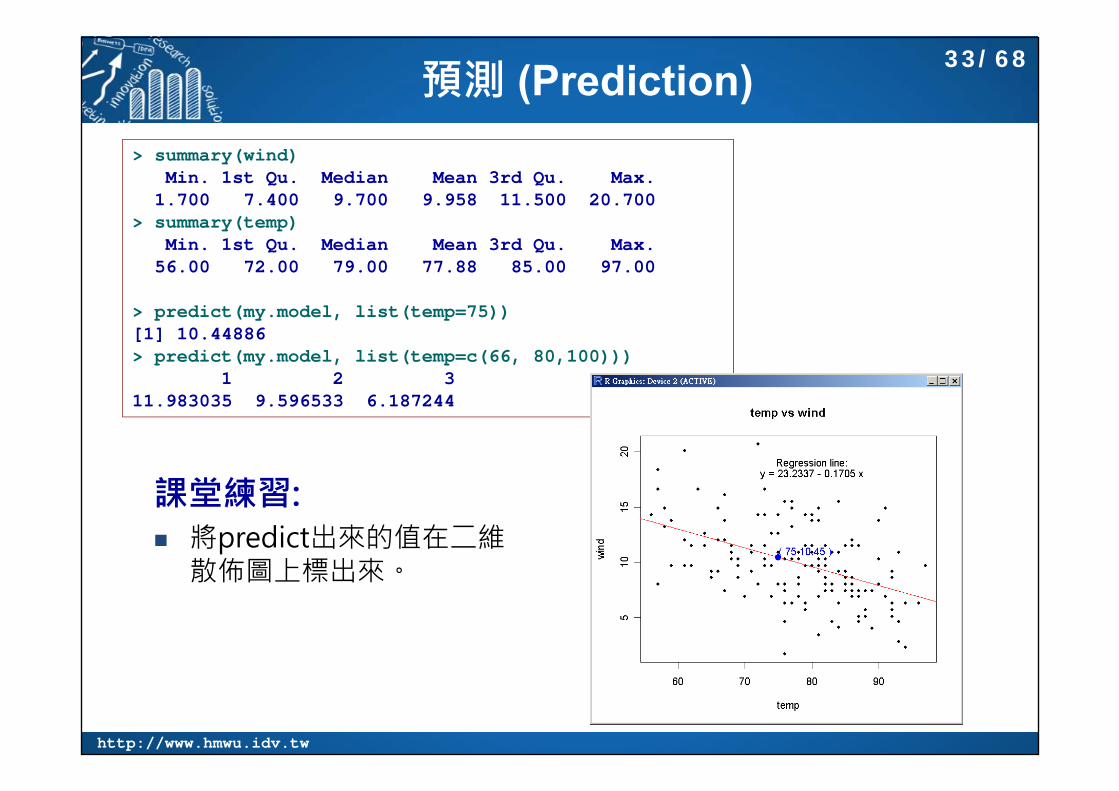
預測 (Prediction)
課堂練習: 將predict出來的值在二維
散佈圖上標出來。
> summary(wind)Min. 1st Qu. Median Mean 3rd Qu. Max. 1.700 7.400 9.700 9.958 11.500 20.700
> summary(temp)Min. 1st Qu. Median Mean 3rd Qu. Max. 56.00 72.00 79.00 77.88 85.00 97.00
> predict(my.model, list(temp=75))[1] 10.44886> predict(my.model, list(temp=c(66, 80,100)))
1 2 3 11.983035 9.596533 6.187244
33/68

http://www.hmwu.idv.tw
統計模型檢測 (Model Checking in R) After fitting a model to data we need to investigate how well the
model describes the data to see if there are any systematic trendsin the goodness of fit.
We hope that ε ~N(0,σ2 I), but Errors may be heterogeneous (unequal variance). Errors may be correlated. Errors may not be normally distributed. (less serious, the βhat's will tend to normality due to
the power of the central limit theorem. With larger datasets, normality of the data is not much of a problem.
“Essentially, all models are wrong, but some are useful”https://en.wikipedia.org/wiki/All_models_are_wrong
Box married Joan Fisher, the second of R.A. Fisher (1890-1962) five daughters.
George Box (1919-2013), Professor Emeritus of Statistics, University of Wisconsin-Madison
34/68
http://www.hmwu.idv.tw
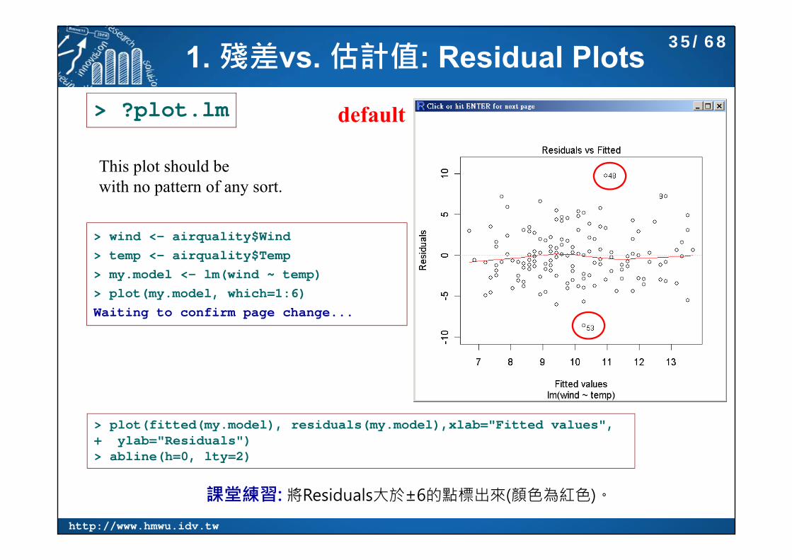
1. 殘差vs. 估計值: Residual Plots
default
> plot(fitted(my.model), residuals(my.model),xlab="Fitted values", + ylab="Residuals")> abline(h=0, lty=2)
This plot should be with no pattern of any sort.
課堂練習: 將Residuals大於±6的點標出來(顏色為紅色)。
> wind <- airquality$Wind> temp <- airquality$Temp> my.model <- lm(wind ~ temp)> plot(my.model, which=1:6)Waiting to confirm page change...
> ?plot.lm
35/68
http://www.hmwu.idv.tw
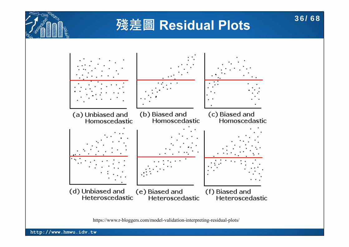
殘差圖 Residual Plots
https://www.r-bloggers.com/model-validation-interpreting-residual-plots/
36/68
http://www.hmwu.idv.tw
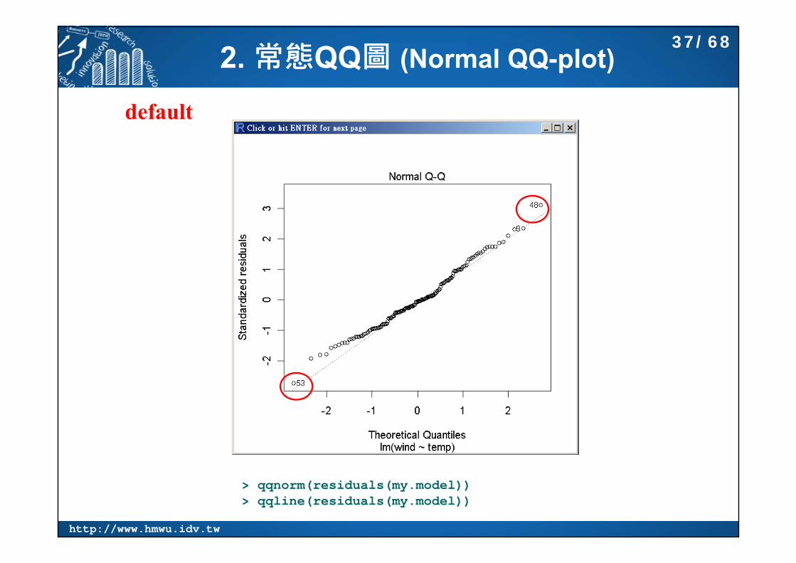
2. 常態QQ圖 (Normal QQ-plot)
default
> qqnorm(residuals(my.model))> qqline(residuals(my.model))
37/68

http://www.hmwu.idv.tw
3. 尺度-位置圖 (A Scale-Location Plot) A scale-loaction plot of sqrt(abs(residuals)) against fitted values. This is like a positive-valued version of the first graph; it is good
for detecting non-constancy of variance (heteroscedasticity).
default
38/68

http://www.hmwu.idv.tw
4. Plot of Cook's Distance vs Row Labels Cook's distance measures the effect of deleting a given observation. Cook's distance is a measure of the squared distance between the least
square estimate based on all n points β and the estimate obtained by deleting the ith points β(i).
Points with a Cook's distance of 1 or more are considered to be influential.
課堂練習: 算出Cook's Distance。 畫出Cook's Distance vs. Row Labels的散
佈圖。 標出前三大Cook's Distance值所在位置。
39/68
2

http://www.hmwu.idv.tw
5. Plot of Residuals vs Leverages Outliers in the response variable are called outliers. Outliers with respect to the predictors are called leverage points. For the regression, it is the points that have large leverage are important. Points that have small leverage “do not count” in the regression – we
could move them or remove them from the data and the regression line does not change very much.
default
課堂練習 : 算出Leverages 。 將Residuals標準化。 畫出Residuals標準化 vs. Leverages
的散佈圖。 標出前三大Leverages值所在位置。
40/68
http://www.hmwu.idv.tw
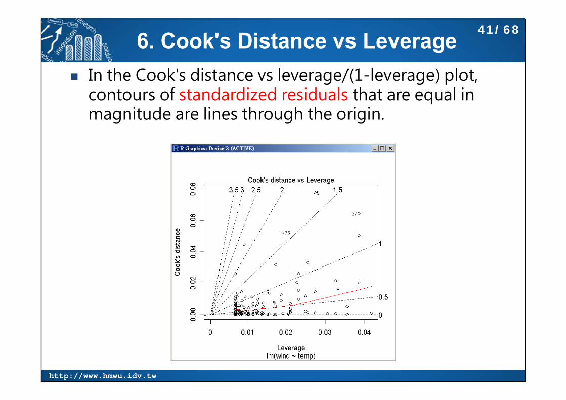
6. Cook's Distance vs Leverage In the Cook's distance vs leverage/(1-leverage) plot,
contours of standardized residuals that are equal in magnitude are lines through the origin.
41/68

http://www.hmwu.idv.tw
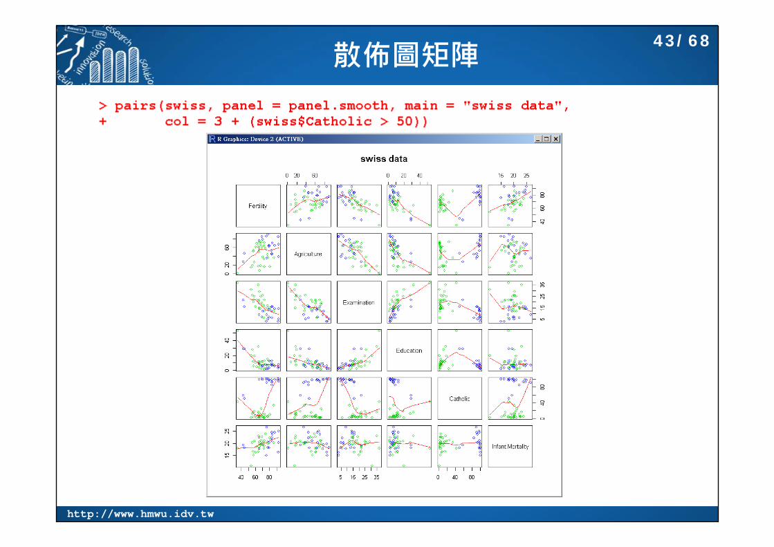
範例: 模型選取/變數選取Swiss Fertility and Socioeconomic Indicators (1888) Data
A data frame with 47 observations on 6 variables, each of which is in percent, i.e., in [0, 100].
[,1] Fertility Ig, ‘common standardized fertility measure’
[,2] Agriculture % of males involved in agriculture as occupation
[,3] Examination % draftees receiving highest mark on army examination
[,4] Education % education beyond primary school for draftees.
[,5] Catholic % ‘catholic’(as opposed to ‘protestant’).
[,6] Infant.Mortality live births who live less than 1 year.
All variables but ‘Fertility’ give proportions of the population.
> head(swiss)Fertility Agriculture Examination Education Catholic Infant.Mortality
Courtelary 80.2 17.0 15 12 9.96 22.2Delemont 83.1 45.1 6 9 84.84 22.2Franches-Mnt 92.5 39.7 5 5 93.40 20.2Moutier 85.8 36.5 12 7 33.77 20.3Neuveville 76.9 43.5 17 15 5.16 20.6Porrentruy 76.1 35.3 9 7 90.57 26.6
42/68
http://www.hmwu.idv.tw
散佈圖矩陣43/68

http://www.hmwu.idv.tw
配適多重迴歸模型: lm 44/68
http://www.hmwu.idv.tw
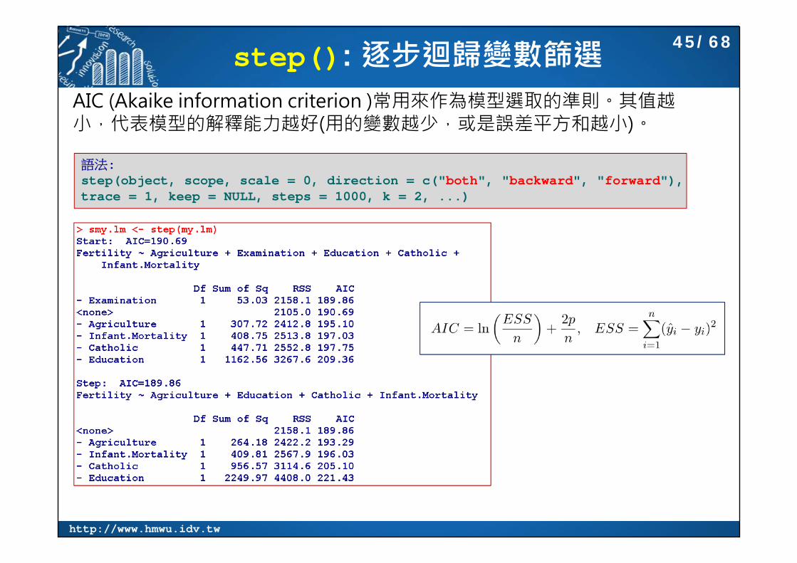
step(): 逐步迴歸變數篩選AIC (Akaike information criterion )常用來作為模型選取的準則。其值越小,代表模型的解釋能力越好(用的變數越少,或是誤差平方和越小)。
語法:step(object, scope, scale = 0, direction = c("both", "backward", "forward"), trace = 1, keep = NULL, steps = 1000, k = 2, ...)
45/68

http://www.hmwu.idv.tw
最後選取的模型46/68

http://www.hmwu.idv.tw
範例: Linear Regression Australian CPI (Consumer Price Index) data, which are quarterly
CPIs from 2008 to 2010. From Australian Bureau of Statistics (http://www.abs.gov.au )
> year <- rep(2008:2010, each=4)> quarter <- rep(1:4, 3)> cpi <- c(162.2, 164.6, 166.5, 166.0,+ 166.2, 167.0, 168.6, 169.5,+ 171.0, 172.1, 173.3, 174.0)> cbind(cpi, year, quarter)
cpi year quarter[1,] 162.2 2008 1[2,] 164.6 2008 2[3,] 166.5 2008 3[4,] 166.0 2008 4[5,] 166.2 2009 1[6,] 167.0 2009 2[7,] 168.6 2009 3[8,] 169.5 2009 4[9,] 171.0 2010 1
[10,] 172.1 2010 2[11,] 173.3 2010 3[12,] 174.0 2010 4> plot(cpi, xaxt="n", ylab="CPI", xlab="")> axis(1, labels=paste(year, quarter, sep="Q"), at=1:12, las=3) # las=3: vertical text.
> cor(year, cpi)[1] 0.9096316> cor(quarter, cpi)[1] 0.3738028
Source: R and Data Mining: Examples and Case Studies, Chapter 5: Regression
47/68
http://www.hmwu.idv.tw
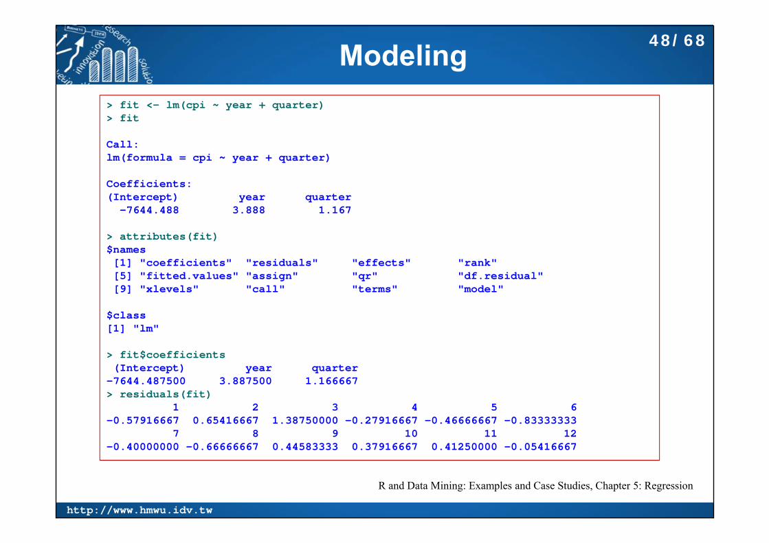
Modeling> fit <- lm(cpi ~ year + quarter)> fit
Call:lm(formula = cpi ~ year + quarter)
Coefficients:(Intercept) year quarter
-7644.488 3.888 1.167
> attributes(fit)$names[1] "coefficients" "residuals" "effects" "rank" [5] "fitted.values" "assign" "qr" "df.residual" [9] "xlevels" "call" "terms" "model"
$class[1] "lm"
> fit$coefficients(Intercept) year quarter
-7644.487500 3.887500 1.166667 > residuals(fit)
1 2 3 4 5 6 -0.57916667 0.65416667 1.38750000 -0.27916667 -0.46666667 -0.83333333
7 8 9 10 11 12 -0.40000000 -0.66666667 0.44583333 0.37916667 0.41250000 -0.05416667
R and Data Mining: Examples and Case Studies, Chapter 5: Regression
48/68
http://www.hmwu.idv.tw
Summary of Fit
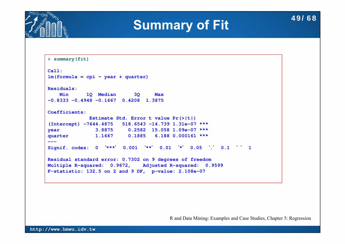
> summary(fit)
Call:lm(formula = cpi ~ year + quarter)
Residuals:Min 1Q Median 3Q Max
-0.8333 -0.4948 -0.1667 0.4208 1.3875
Coefficients:Estimate Std. Error t value Pr(>|t|)
(Intercept) -7644.4875 518.6543 -14.739 1.31e-07 ***year 3.8875 0.2582 15.058 1.09e-07 ***quarter 1.1667 0.1885 6.188 0.000161 ***---Signif. codes: 0 ‘***’ 0.001 ‘**’ 0.01 ‘*’ 0.05 ‘.’ 0.1 ‘ ’ 1
Residual standard error: 0.7302 on 9 degrees of freedomMultiple R-squared: 0.9672, Adjusted R-squared: 0.9599 F-statistic: 132.5 on 2 and 9 DF, p-value: 2.108e-07
R and Data Mining: Examples and Case Studies, Chapter 5: Regression
49/68

http://www.hmwu.idv.tw
Model Diagnostic
R and Data Mining: Examples and Case Studies, Chapter 5: Regression
> plot(fit)
50/68

http://www.hmwu.idv.tw
Plot of Fit> library(scatterplot3d)> s3d <- scatterplot3d(year, quarter, cpi, highlight.3d=T, type="h", lab=c(2,3))> s3d$plane3d(fit)
R and Data Mining: Examples and Case Studies, Chapter 5: Regression
51/68

http://www.hmwu.idv.tw
Prediction> data2011 <- data.frame(year=2011, quarter=1:4)> cpi2011 <- predict(fit, newdata=data2011)> cpi2011
1 2 3 4 174.4417 175.6083 176.7750 177.9417> style <- c(rep(1,12), rep(2,4))> plot(c(cpi, cpi2011), xaxt="n", ylab="CPI", xlab="", pch=style, col=style)> axis(1, at=1:16, las=3, labels=c(paste(year, quarter, sep="Q"), "2011Q1", "2011Q2", "2011Q3", "2011Q4"))
R and Data Mining: Examples and Case Studies, Chapter 5: Regression
52/68
http://www.hmwu.idv.tw
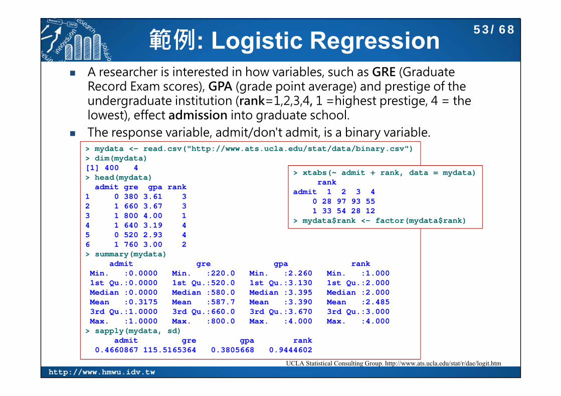
範例: Logistic Regression A researcher is interested in how variables, such as GRE (Graduate
Record Exam scores), GPA (grade point average) and prestige of the undergraduate institution (rank=1,2,3,4, 1 =highest prestige, 4 = the lowest), effect admission into graduate school.
The response variable, admit/don't admit, is a binary variable.
UCLA Statistical Consulting Group. http://www.ats.ucla.edu/stat/r/dae/logit.htm
> mydata <- read.csv("http://www.ats.ucla.edu/stat/data/binary.csv")> dim(mydata)[1] 400 4> head(mydata)
admit gre gpa rank1 0 380 3.61 32 1 660 3.67 33 1 800 4.00 14 1 640 3.19 45 0 520 2.93 46 1 760 3.00 2> summary(mydata)
admit gre gpa rank Min. :0.0000 Min. :220.0 Min. :2.260 Min. :1.000 1st Qu.:0.0000 1st Qu.:520.0 1st Qu.:3.130 1st Qu.:2.000 Median :0.0000 Median :580.0 Median :3.395 Median :2.000 Mean :0.3175 Mean :587.7 Mean :3.390 Mean :2.485 3rd Qu.:1.0000 3rd Qu.:660.0 3rd Qu.:3.670 3rd Qu.:3.000 Max. :1.0000 Max. :800.0 Max. :4.000 Max. :4.000
> sapply(mydata, sd)admit gre gpa rank
0.4660867 115.5165364 0.3805668 0.9444602
> xtabs(~ admit + rank, data = mydata)rank
admit 1 2 3 40 28 97 93 551 33 54 28 12
> mydata$rank <- factor(mydata$rank)
53/68
http://www.hmwu.idv.tw
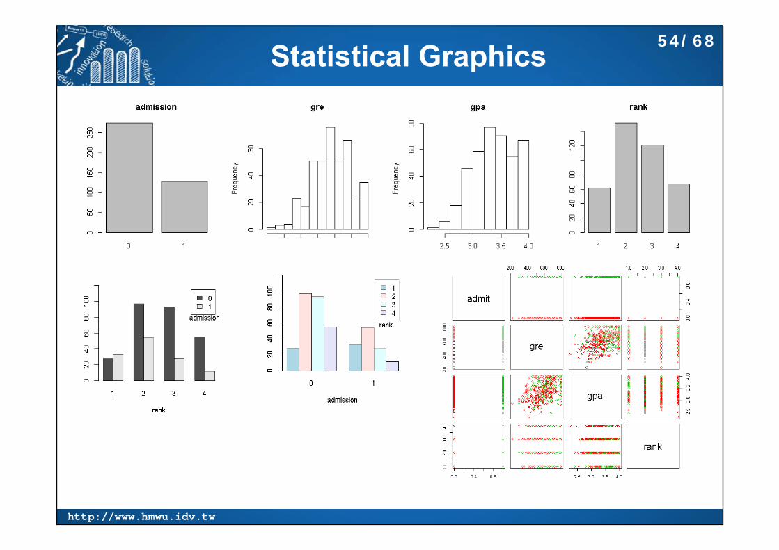
Statistical Graphics 54/68
http://www.hmwu.idv.tw
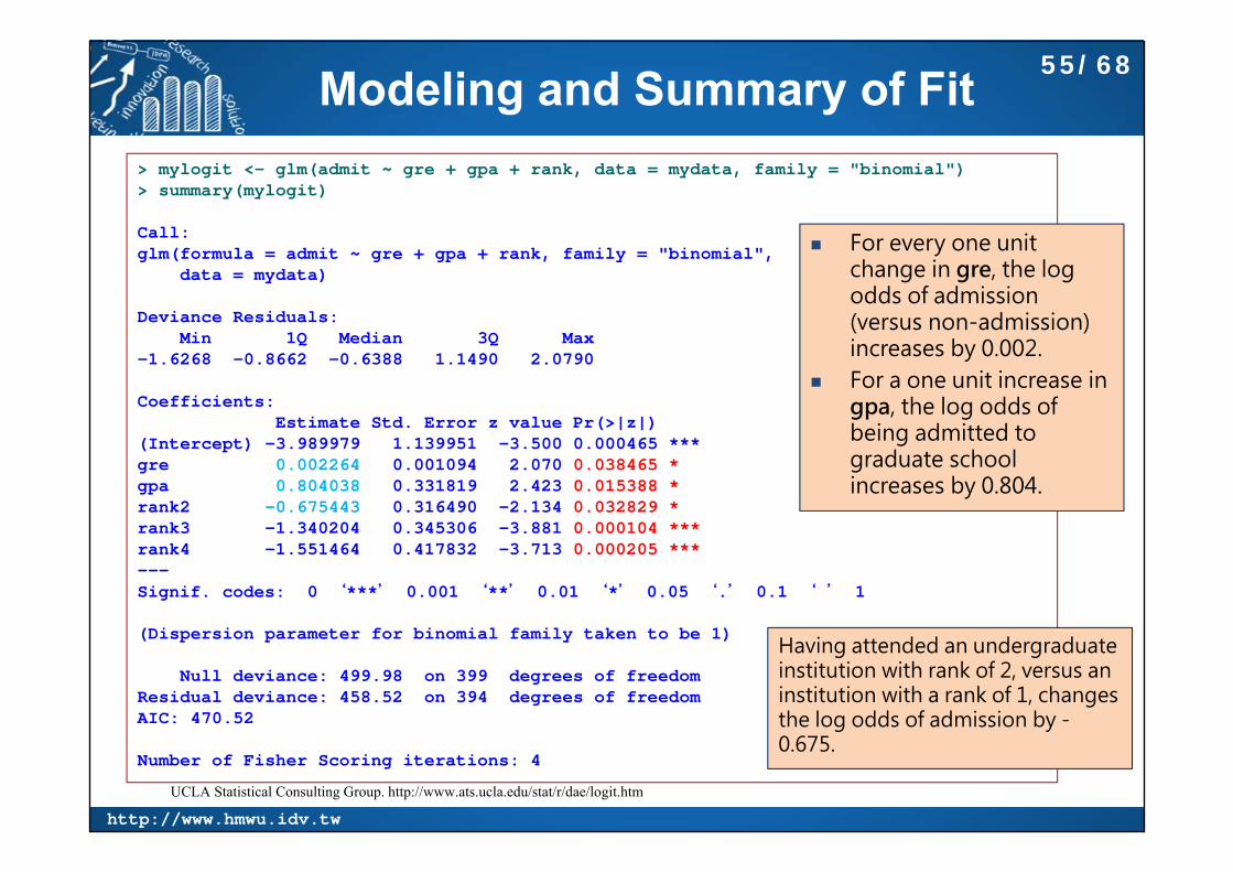
Modeling and Summary of Fit> mylogit <- glm(admit ~ gre + gpa + rank, data = mydata, family = "binomial")> summary(mylogit)
Call:glm(formula = admit ~ gre + gpa + rank, family = "binomial",
data = mydata)
Deviance Residuals: Min 1Q Median 3Q Max
-1.6268 -0.8662 -0.6388 1.1490 2.0790
Coefficients:Estimate Std. Error z value Pr(>|z|)
(Intercept) -3.989979 1.139951 -3.500 0.000465 ***gre 0.002264 0.001094 2.070 0.038465 * gpa 0.804038 0.331819 2.423 0.015388 *rank2 -0.675443 0.316490 -2.134 0.032829 *rank3 -1.340204 0.345306 -3.881 0.000104 ***rank4 -1.551464 0.417832 -3.713 0.000205 ***---Signif. codes: 0 ‘***’ 0.001 ‘**’ 0.01 ‘*’ 0.05 ‘.’ 0.1 ‘ ’ 1
(Dispersion parameter for binomial family taken to be 1)
Null deviance: 499.98 on 399 degrees of freedomResidual deviance: 458.52 on 394 degrees of freedomAIC: 470.52
Number of Fisher Scoring iterations: 4
Having attended an undergraduate institution with rank of 2, versus an institution with a rank of 1, changes the log odds of admission by -0.675.
UCLA Statistical Consulting Group. http://www.ats.ucla.edu/stat/r/dae/logit.htm
55/68
For every one unit change in gre, the log odds of admission (versus non-admission) increases by 0.002.
For a one unit increase in gpa, the log odds of being admitted to graduate school increases by 0.804.

http://www.hmwu.idv.tw
Wald Test for Model Coefficients
Sigma: the variance covariance matrix of the error terms, b: the coefficients, Terms: terms in the model are to be tested, in this case, terms 4, 5, and 6, are the three terms for the levels of rank.
The difference between the coefficient for rank=2 and the coefficient for rank=3 is statistically significant.
> library(aod) #aod: Analysis of Overdispersed Data> wald.test(b = coef(mylogit), Sigma = vcov(mylogit), Terms = 4:6)Wald test:----------
Chi-squared test:X2 = 20.9, df = 3, P(> X2) = 0.00011
> l <- cbind(0,0,0,1,-1,0)> wald.test(b = coef(mylogit), Sigma = vcov(mylogit), L = l)Wald test:----------
Chi-squared test:X2 = 5.5, df = 1, P(> X2) = 0.019
wald.test(Sigma, b, Terms = NULL, L = NULL, H0 = NULL, df = NULL, verbose = FALSE)
To contrast two terms, we multiply one of them by 1, and the other by -1. The other terms in the model are not involved in the test, so they are multiplied by 0. Test the difference (subtraction) of the terms for rank=2 and rank=3 (i.e., the 4th and 5th terms in the model). L=l: base the test on the vector l (rather than using the Terms option).
UCLA Statistical Consulting Group. http://www.ats.ucla.edu/stat/r/dae/logit.htm
56/68

http://www.hmwu.idv.tw
Interpret Coefficients as Odds-ratios
For a one unit increase in gpa, the odds of being admitted to graduate school (versus not being admitted) increase by a factor of 2.23.
For more information on interpreting odds ratios see our FAQ page How do I interpret odds ratios in logistic regression? http://www.ats.ucla.edu/stat/mult_pkg/faq/general/odds_ratio.htm
Note that while R produces it, the odds ratio for the intercept is not generally interpreted.
> exp(cbind(OR = coef(mylogit), confint(mylogit)))Waiting for profiling to be done...
OR 2.5 % 97.5 %(Intercept) 0.0185001 0.001889165 0.1665354gre 1.0022670 1.000137602 1.0044457gpa 2.2345448 1.173858216 4.3238349rank2 0.5089310 0.272289674 0.9448343rank3 0.2617923 0.131641717 0.5115181rank4 0.2119375 0.090715546 0.4706961
http://www.ats.ucla.edu/stat/r/dae/logit.htm
57/68

http://www.hmwu.idv.tw
Predicted Probabilities
The predicted probability of being accepted into a graduate program is 0.52 for students from the highest prestige undergraduate institutions (rank=1), and 0.18 for students from the lowest ranked institutions (rank=4), holding gre and gpa at their means.
> newdata1 <- with(mydata, data.frame(gre = mean(gre), gpa = mean(gpa), rank = factor(1:4)))> newdata1
gre gpa rank1 587.7 3.3899 12 587.7 3.3899 23 587.7 3.3899 34 587.7 3.3899 4> newdata1$rankP <- predict(mylogit, newdata = newdata1, type = "response")> newdata1
gre gpa rank rankP1 587.7 3.3899 1 0.51660162 587.7 3.3899 2 0.35228463 587.7 3.3899 3 0.21861204 587.7 3.3899 4 0.1846684
http://www.ats.ucla.edu/stat/r/dae/logit.htm
Predicted probabilities can be computed for both categorical and continuous predictor variables.
Want to calculate the predicted probability of admission at each value of rank, holding gre and gpa at their means.
58/68

http://www.hmwu.idv.tw
Create a Table of Predicted Probabilities > newdata2 <- with(mydata,+ data.frame(gre = rep(seq(from = 200, to = 800, length.out = 100), 4),+ gpa = mean(gpa), rank = factor(rep(1:4, each = 100))))> dim(newdata2)[1] 400 3> head(newdata2)
gre gpa rank1 200.0000 3.3899 12 206.0606 3.3899 13 212.1212 3.3899 14 218.1818 3.3899 15 224.2424 3.3899 16 230.3030 3.3899 1> > newdata3 <- cbind(newdata2, predict(mylogit, newdata = newdata2, type="link", se=TRUE))> newdata3 <- within(newdata3, {+ PredictedProb <- plogis(fit)+ LL <- plogis(fit - (1.96 * se.fit))+ UL <- plogis(fit + (1.96 * se.fit))+ })> head(newdata3)
gre gpa rank fit se.fit residual.scale UL LL PredictedProb1 200.0000 3.3899 1 -0.8114870 0.5147714 1 0.5492064 0.1393812 0.30757372 206.0606 3.3899 1 -0.7977632 0.5090986 1 0.5498513 0.1423880 0.31050423 212.1212 3.3899 1 -0.7840394 0.5034491 1 0.5505074 0.1454429 0.31344994 218.1818 3.3899 1 -0.7703156 0.4978239 1 0.5511750 0.1485460 0.31641085 224.2424 3.3899 1 -0.7565919 0.4922237 1 0.5518545 0.1516973 0.31938676 230.3030 3.3899 1 -0.7428681 0.4866494 1 0.5525464 0.1548966 0.3223773
Create 100 values of gre between 200 and 800, at each value of rank (i.e., 1, 2, 3, and 4) and plot.
http://www.ats.ucla.edu/stat/r/dae/logit.htm
59/68
http://www.hmwu.idv.tw
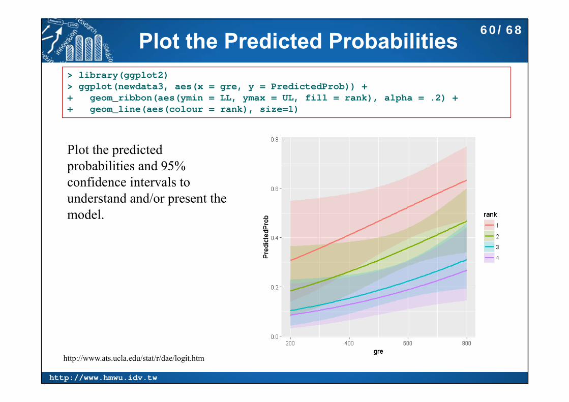
Plot the Predicted Probabilities> library(ggplot2) > ggplot(newdata3, aes(x = gre, y = PredictedProb)) ++ geom_ribbon(aes(ymin = LL, ymax = UL, fill = rank), alpha = .2) ++ geom_line(aes(colour = rank), size=1)
Plot the predicted probabilities and 95% confidence intervals to understand and/or present the model.
http://www.ats.ucla.edu/stat/r/dae/logit.htm
60/68
http://www.hmwu.idv.tw
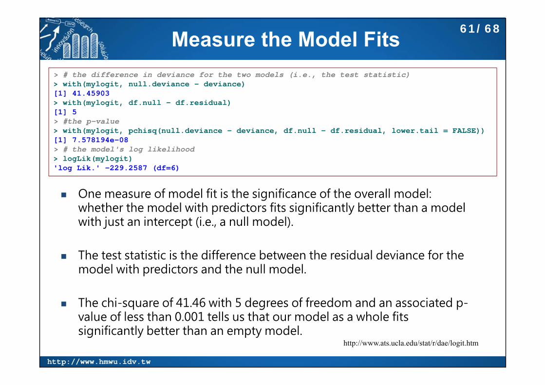
Measure the Model Fits
One measure of model fit is the significance of the overall model: whether the model with predictors fits significantly better than a model with just an intercept (i.e., a null model).
The test statistic is the difference between the residual deviance for the model with predictors and the null model.
The chi-square of 41.46 with 5 degrees of freedom and an associated p-value of less than 0.001 tells us that our model as a whole fits significantly better than an empty model.
> # the difference in deviance for the two models (i.e., the test statistic)> with(mylogit, null.deviance - deviance)[1] 41.45903> with(mylogit, df.null - df.residual)[1] 5> #the p-value> with(mylogit, pchisq(null.deviance - deviance, df.null - df.residual, lower.tail = FALSE))[1] 7.578194e-08> # the model's log likelihood> logLik(mylogit)'log Lik.' -229.2587 (df=6)
http://www.ats.ucla.edu/stat/r/dae/logit.htm
61/68
http://www.hmwu.idv.tw
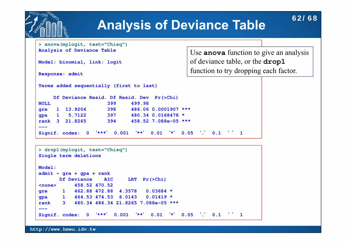
Analysis of Deviance Table> anova(mylogit, test="Chisq")Analysis of Deviance Table
Model: binomial, link: logit
Response: admit
Terms added sequentially (first to last)
Df Deviance Resid. Df Resid. Dev Pr(>Chi) NULL 399 499.98 gre 1 13.9204 398 486.06 0.0001907 ***gpa 1 5.7122 397 480.34 0.0168478 * rank 3 21.8265 394 458.52 7.088e-05 ***---Signif. codes: 0 ‘***’ 0.001 ‘**’ 0.01 ‘*’ 0.05 ‘.’ 0.1 ‘ ’ 1
> drop1(mylogit, test="Chisq")Single term deletions
Model:admit ~ gre + gpa + rank
Df Deviance AIC LRT Pr(>Chi) <none> 458.52 470.52 gre 1 462.88 472.88 4.3578 0.03684 * gpa 1 464.53 474.53 6.0143 0.01419 * rank 3 480.34 486.34 21.8265 7.088e-05 ***---Signif. codes: 0 ‘***’ 0.001 ‘**’ 0.01 ‘*’ 0.05 ‘.’ 0.1 ‘ ’ 1
Use anova function to give an analysis of deviance table, or the drop1function to try dropping each factor.
62/68
http://www.hmwu.idv.tw
Things to Consider Empty cells or small cells: check the crosstab between categorical
predictors and the outcome variable. If a cell has very few cases (a small cell), the model may become unstable or it might not run at all.
Separation or quasi-separation (also called perfect prediction), a condition in which the outcome does not vary at some levels of the independent variables. See http://www.ats.ucla.edu/stat/mult_pkg/faq/general/complete_separation_logit_models.htm
Sample size: Both logit and probit models require more cases than OLS regression because they use maximum likelihood estimation techniques.
Pseudo-R-squared: none of psuedo-R-squared measures can be interpreted exactly as R-squared in OLS regression is interpreted. See http://www.ats.ucla.edu/stat/mult_pkg/faq/general/Psuedo_RSquareds.htm
Diagnostics: The diagnostics for logistic regression are different from those for OLS regression. See Hosmer and Lemeshow (2000, Chapter 5).
http://www.ats.ucla.edu/stat/r/dae/logit.htm
63/68

http://www.hmwu.idv.tw
共線性 (Collinearity) What is the multicollinearity (collinearity)
it is a statistical phenomenon in which two or more predictor variables in a multiple regression model are highly correlated.
one predictor can be linearly predicted from the others with a non-trivial degree of accuracy.
How problematic is multicollinearity? Moderate multicollinearity may not be problematic. Severe multicollinearity can increase the variance of the coefficient
estimates and make the estimates very sensitive to minor changes in the model: the coefficient estimates are unstable (may be to switch signs) and difficult to
interpret, or parameter estimates may include substantial amounts of uncertainty, forward or backward selection of variables could produce inconsistent results, variance partitioning analyses may be unable to identify unique sources of
variation.
64/68

http://www.hmwu.idv.tw
變異數膨脹因子The Variance Inflation Factors
A VIF for a single explanatory variable is obtained using the R-squared value of the regression of that variable Xj against all other explanatory variables.
A VIF measures how much the variance of the estimated regression coefficients are inflated as compared to when the predictor variables are not linearly related.
65/68

http://www.hmwu.idv.tw
vif in R R packages:
vif{faraway}, vif{HH}, vif{car}, VIF{fmsb}, vif{VIF} faraway: Functions and Datasets for Books by Julian Faraway HH: Statistical Analysis and Data Display: Heiberger and Holland car: Companion to Applied Regression fmsb: Functions for Medical Statistics Book with some Demographic Data VIF: A Fast Regression Algorithm For Large Data
> head(airquality)Ozone Solar.R Wind Temp Month Day
1 41 190 7.4 67 5 12 36 118 8.0 72 5 23 12 149 12.6 74 5 34 18 313 11.5 62 5 45 NA NA 14.3 56 5 56 28 NA 14.9 66 5 6> > model0 <- lm(Ozone ~ Wind + Temp + Solar.R, data=airquality)
66/68
http://www.hmwu.idv.tw
An Example
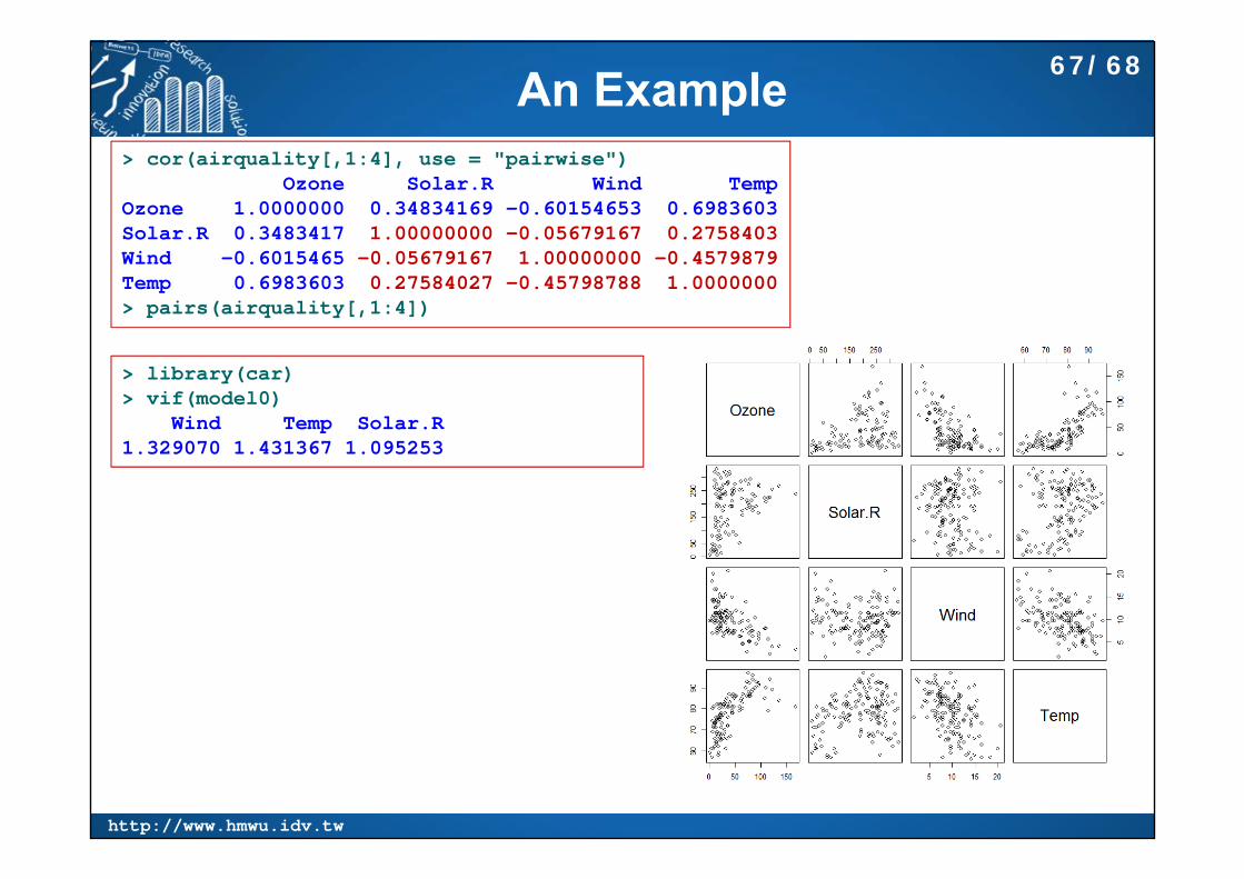
> library(car)> vif(model0)
Wind Temp Solar.R 1.329070 1.431367 1.095253
> cor(airquality[,1:4], use = "pairwise")Ozone Solar.R Wind Temp
Ozone 1.0000000 0.34834169 -0.60154653 0.6983603Solar.R 0.3483417 1.00000000 -0.05679167 0.2758403Wind -0.6015465 -0.05679167 1.00000000 -0.4579879Temp 0.6983603 0.27584027 -0.45798788 1.0000000> pairs(airquality[,1:4])
67/68

http://www.hmwu.idv.tw
The Stepwise VIF Selection> summary(model0)Call:lm(formula = Ozone ~ Wind + Temp + Solar.R, data = airquality)
Residuals:Min 1Q Median 3Q Max
-40.485 -14.219 -3.551 10.097 95.619
Coefficients:Estimate Std. Error t value Pr(>|t|)
(Intercept) -64.34208 23.05472 -2.791 0.00623 ** Wind -3.33359 0.65441 -5.094 1.52e-06 ***Temp 1.65209 0.25353 6.516 2.42e-09 ***Solar.R 0.05982 0.02319 2.580 0.01124 * ---Signif. codes: 0 ‘***’ 0.001 ‘**’ 0.01 ‘*’ 0.05 ‘.’ 0.1 ‘ ’ 1
Residual standard error: 21.18 on 107 degrees of freedom(42 observations deleted due to missingness)
Multiple R-squared: 0.6059, Adjusted R-squared: 0.5948 F-statistic: 54.83 on 3 and 107 DF, p-value: < 2.2e-16
> library(fmsb)> model1 <- lm(Wind ~ Temp + Solar.R, data=airquality)> model2 <- lm(Temp ~ Wind + Solar.R, data=airquality)> model3 <- lm(Solar.R ~ Wind + Temp, data=airquality)> # checking multicolinearity for independent variables.> VIF(model0)[1] 2.537392> sapply(list(model1, model2, model3), VIF)[1] 1.267492 1.367450 1.089300
68/68

http://www.hmwu.idv.tw
69/68
https://www.r-bloggers.com/machine-learning-linear-regression-full-example-boston-housing/?utm_source=feedburner&utm_medium=email&utm_campaign=Feed%3A+RBloggers+%28R+bloggers%29
Machine Learning. Linear Regression Full Example (Boston Housing).