chapter transient response analys es · א ˘ jj jj א ˇ ˆ˙˝א א˛˚˜ eeee٣٥١١...

��א�� א�� א�� א�� J� J� J� Jא��א��א��א�� א��א�� א��א�� א��א�� א��א��

� � ��א�"�!��א�"�! � �&%$��א�"#��א�"�! � �&%$��א�"#��א�"�! � �&%$��א�"#�FFFF��٣٥١١٣٥١١٣٥١١٣٥١١EEEE&%$��א�"#

,,,,�K�K�K�K.�/� 012��3&.�/� 012��3&.�/� 012��3&.�/� 012��3&

1 Dr. AHMED MUSTAFA HUSSEIN

CHAPTER # 6 TRANSIENT RESPONSE ANALYSES

1. Introduction

It was stated previously in lecture #1 that the first step in analyzing a control system

was to derive a mathematical model of the system. Once such a model is obtained,

various methods are available for the analysis of system performance.

Typical Test Signals: The commonly used test input signals are those of step

functions, ramp functions, acceleration functions, impulse functions, sinusoidal

functions, and the like. With these test signals, mathematical and experimental

analyses of control systems can be carried out easily since the signals are very simple

functions of time.

If the inputs to a control system are gradually changing functions of time, then a ramp

function of time may be a good test signal. Similarly, if a system is subjected to

sudden disturbances, a step function of time may be a good test signal; and for a

system subjected to shock inputs, an impulse function may be best. Once a control

system is designed on the basis of test signals, the performance of the system in



,,,,�K�K�K�K.�/� 012��3&.�/� 012��3&.�/� 012��3&.�/� 012��3&


response to actual inputs is generally satisfactory. The use of such test signals enables

one to compare the performance of all systems on the same basis.

The time response of a control system consists of two parts as shown in Fig. 1;

a) Transient response

b) Steady-state response.

Fig. 1, Time response

By transient response, we mean that which goes from the initial state to the final

state.

By steady-state response, we mean the manner in which the system output behaves as

t approaches infinity. Thus the system response C(t) may be written as

where Ctr(t) is the transient response and Css(t) is the steady-state response.

The transient response of a practical control system often exhibits damped

oscillations before reaching a steady state. If the output of a system at steady state

does not exactly agree with the input, the system is said to have steady state error.

This error is indicative of the accuracy of the system. In analyzing a control system,

we must examine transient-response behavior and steady-state behavior.



,,,,�K�K�K�K.�/� 012��3&.�/� 012��3&.�/� 012��3&.�/� 012��3&


2. Transient Response

2.1 First-Order system

Consider the first-order system shown in Fig. 2.

Fig. 2, Block diagram and its simplification

The input-output relationship is given by

For a unit step input whose Laplace transform is 1/S, the output C(S) is given by

Using partial fraction,

Taking the inverse Laplace transform

The above equation indicates that initially (at t = 0) the output c(t) is zero and finally

(at t = ∞) it becomes unity as shown in Fig. 3.

Fig. 3. Time response of a first-order system



,,,,�K�K�K�K.�/� 012��3&.�/� 012��3&.�/� 012��3&.�/� 012��3&


One important characteristic of such an exponential response curve c(t) is that at t = T

the value of c(t) is 0.632, or the response c(t) has reached 63.2% of its final value.

This may be easily seen by substituting t = T in c(t). That is,

By the same way, in two time constants (t = 2T), the response reaches 86.5% of the

final value. At t = 3T, the response reaches 95% of its final value. At t = 4T, the

system response reaches 98.2% of its final value. Finally at t = 5T, the response

reaches 99.3% of the final value. Thus, for t ≥ 4T, the response remains within 2% of

the final value. As seen from the equation of c(t), the steady state value (c(t) = 1) is

reached mathematically only after an infinite time. In practice, however, a reasonable

estimate of the response time is the length of time the response curve needs to reach

and stay within the 2% line of the final value, or four time constants.

2.2 Second-Order Systems

Consider the 2nd

order control system shown in Fig. 4, whose T.F. is given as:

This form is called the standard form of the second-order system, where ζ and ωn are

the damping ratio and undamped natural frequency, respectively.

Fig. 4. Standard form of Second-order control system

For a unit-step input ( R(S) = 1/S ), C(s) can be written

Using partial fraction,



,,,,�K�K�K�K.�/� 012��3&.�/� 012��3&.�/� 012��3&.�/� 012��3&


The frequency ωd, is called the damped natural frequency.

�� = �� 1 −

Taking inverse Laplace for the output C(s),

This result can be obtained directly by using a table of Laplace transforms tables.

If we plot the output C(t) versus time, such kind of plot is dependent on the two

parameters ζ and ωn. A family of curves at different values of ζ is shown in Fig. 5.

Fig. 5. Transient response of 2nd

order system at different ζ.



,,,,�K�K�K�K.�/� 012��3&.�/� 012��3&.�/� 012��3&.�/� 012��3&


The characteristic equation of any 2nd

order system is given by:

Complete square of the above equation we get;

As the parameters ζ changes, the location of the system poles S1 and S2 are change.

Therefore, the dynamic behavior of the second-order system is also changes. The

nature of the roots s1 and s2 of the characteristic equation with varying values of

damping ratio ζ can be shown in the complex plane as shown in Fig. 6.

Fig. 6. Closed loop poles and transient response



,,,,�K�K�K�K.�/� 012��3&.�/� 012��3&.�/� 012��3&.�/� 012��3&


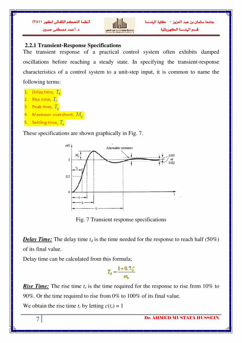
2.2.1 Transient‐‐‐‐Response Specifications

The transient response of a practical control system often exhibits damped

oscillations before reaching a steady state. In specifying the transient‐response

characteristics of a control system to a unit‐step input, it is common to name the

following terms:

These specifications are shown graphically in Fig. 7.

Fig. 7 Transient response specifications

Delay Time: The delay time td is the time needed for the response to reach half (50%)

of its final value.

Delay time can be calculated from this formula;

Rise Time: The rise time tr is the time required for the response to rise from 10% to

90%. Or the time required to rise from 0% to 100% of its final value.

We obtain the rise time tr by letting c(tr) = 1



,,,,�K�K�K�K.�/� 012��3&.�/� 012��3&.�/� 012��3&.�/� 012��3&


Since � � �� ≠ 0, therefore

Where β is defined by Fig. 8, as the angle in radians.

Fig. 8. Definition of angle β

Peak Time: The peak time tp is the time required for the response to reach the first

peak of the overshoot.

We may obtain the peak time by differentiating c(t) with respect to time and letting

this derivative equal zero.

The cosine terms in the above equation cancel each other. Therefore, dc(t)/dt,

evaluated at t = tp, can be simplified to



,,,,�K�K�K�K.�/� 012��3&.�/� 012��3&.�/� 012��3&.�/� 012��3&


This means

Since the peak time corresponds to the first peak overshoot, �� = �

Maximum (percent Overshoot): The maximum percent overshoot Mp is the

maximum peak value of the response curve [the curve of c(t) versus t ], measured

from c (∞) . If c (∞) =1, the maximum percent overshoot is Mp × 100%. If the final

steady state value c (∞) of the response differs from unity, then it is common

practice to use the following definition:

The maximum overshoot occurs at the peak time. Therefore

�� = � � ��

Settling Time: The settling time ts is the time required for the response curve to reach

and stay within ± 2% of the final value. In some cases, 5% instead of 2%, is used as

the percentage of the final value. The settling time is the largest time constant of the

system.

The settling time corresponding to ± 2% or ± 5% tolerance band may be measured in

terms of the time constant {T = l/ (ζ ωn)}



,,,,�K�K�K�K.�/� 012��3&.�/� 012��3&.�/� 012��3&.�/� 012��3&


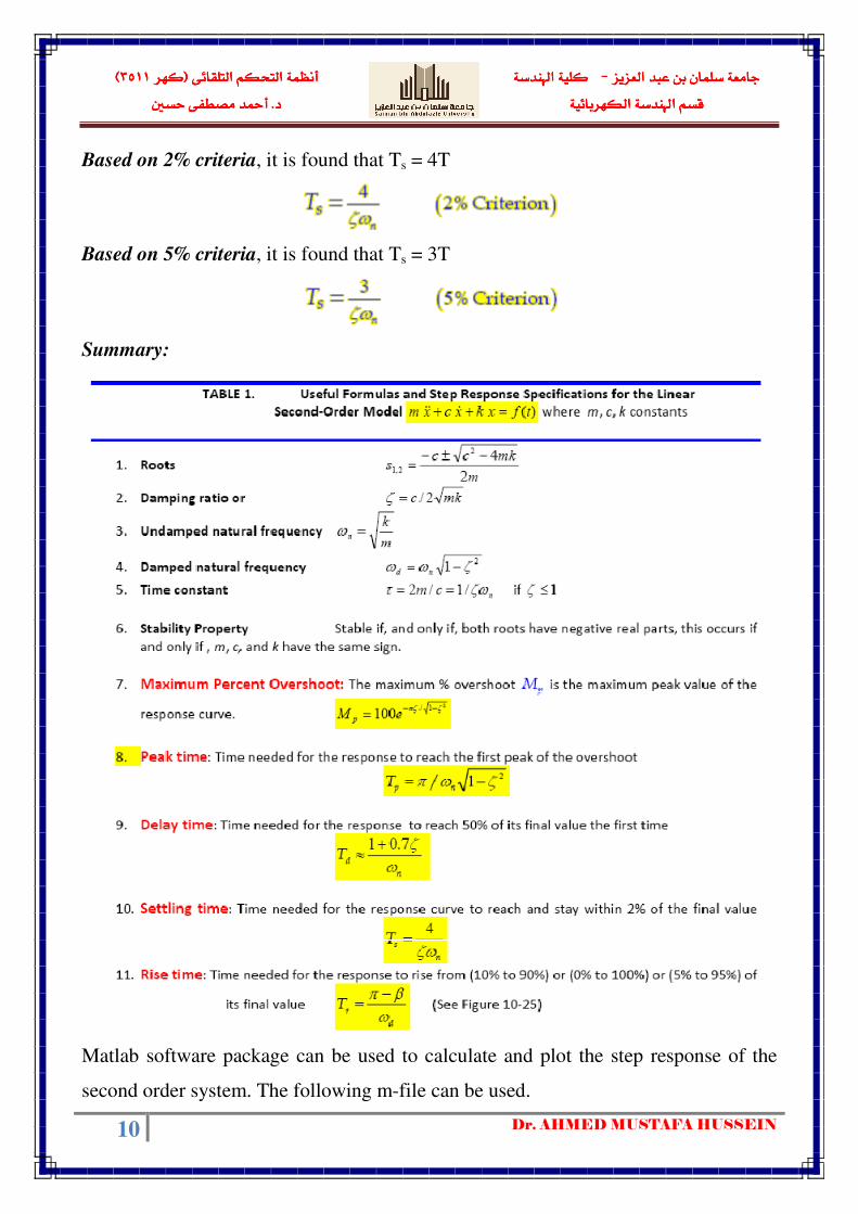
Based on 2% criteria, it is found that Ts = 4T

Based on 5% criteria, it is found that Ts = 3T

Summary:

Matlab software package can be used to calculate and plot the step response of the

second order system. The following m-file can be used.



,,,,�K�K�K�K.�/� 012��3&.�/� 012��3&.�/� 012��3&.�/� 012��3&


Therefore the step response at different value of zeta is given below

In the previous Matlab code we consider some Matlab functions such as tf and step.

What is tf and step? and how can we use them?



,,,,�K�K�K�K.�/� 012��3&.�/� 012��3&.�/� 012��3&.�/� 012��3&


"tf" Specifies a SISO transfer function for model h(s) = n(s)/d(s)

>> h = t f (num, den )

What are num & den?

row vectors listing the coefficients of the polynomials n(s) and d(s) ordered in

descending powers of s

draw the step response of the T.F

�. �. = 100(2� + 1)4� + � + 1

Steady-State Error

The difference between the input and output of a system in the limit as time goes to

infinity, and it will be discussed in more details in next chapter.



,,,,�K�K�K�K.�/� 012��3&.�/� 012��3&.�/� 012��3&.�/� 012��3&


Feedback PID controller – How does it work I?

As shown in the feedback control system given above, the type of controller used is

PID controller. The PID terms are stand for:

P: Proportional,

I: Integral,

D: Derivative



,,,,�K�K�K�K.�/� 012��3&.�/� 012��3&.�/� 012��3&.�/� 012��3&


These correlations may not be exactly accurate, because Kp, Ki, and Kd are

dependent on each other. In fact, changing one of these variables can change the

effect of the other two.

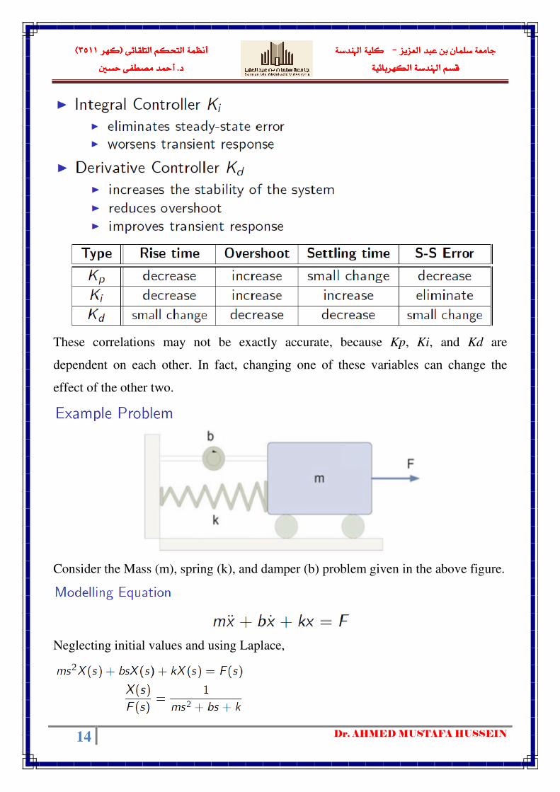
Consider the Mass (m), spring (k), and damper (b) problem given in the above figure.

Neglecting initial values and using Laplace,



,,,,�K�K�K�K.�/� 012��3&.�/� 012��3&.�/� 012��3&.�/� 012��3&


From the system response shown above, the Mass-spring and damper system, is

suffering from the following problems:



,,,,�K�K�K�K.�/� 012��3&.�/� 012��3&.�/� 012��3&.�/� 012��3&


First Trial to solve the system problems is by using Proportional Controller;

Rise time is improved (Tr=0.1) and steady-state error is improved (Ess=0.95) but the

system overshoot is deteriorated (Mp~1.1). Settling time (Ts=1.2)



,,,,�K�K�K�K.�/� 012��3&.�/� 012��3&.�/� 012��3&.�/� 012��3&


Second Trial to solve the system problems is by using Proportional-Derivative

Controller;

Rise time and steady-state error are not affected. But the system overshoot is

improved (Mp~1.05) and settling time is improved (Ts~0.5)



,,,,�K�K�K�K.�/� 012��3&.�/� 012��3&.�/� 012��3&.�/� 012��3&


Third Trial to solve the system problems is by using Proportional-Integral Controller;

It is important to note that: Eliminated steady-state error, decreased over-shoot

But rise and settling times (Tr & Ts) are deteriorated



,,,,�K�K�K�K.�/� 012��3&.�/� 012��3&.�/� 012��3&.�/� 012��3&


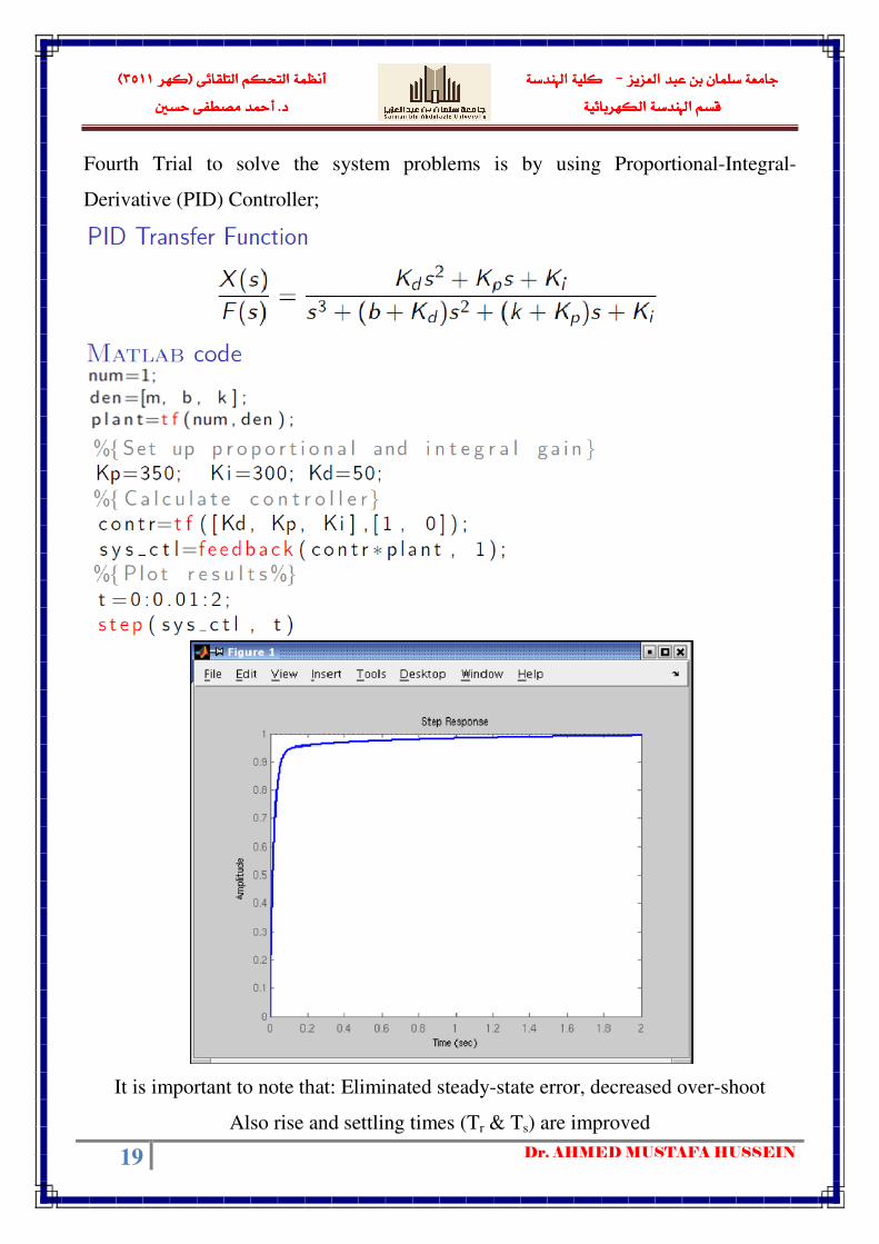
Fourth Trial to solve the system problems is by using Proportional-Integral-

Derivative (PID) Controller;

It is important to note that: Eliminated steady-state error, decreased over-shoot

Also rise and settling times (Tr & Ts) are improved



,,,,�K�K�K�K.�/� 012��3&.�/� 012��3&.�/� 012��3&.�/� 012��3&


Example #1

Consider the system shown in Fig. 9, where ζ = 0.6 and ωn = 5 rad/sec. Let us obtain

the rise time tr, peak time tp, maximum overshoot Mp, and settling time tp when the

system is subjected to a unit-step input.

Fig. 9.



,,,,�K�K�K�K.�/� 012��3&.�/� 012��3&.�/� 012��3&.�/� 012��3&


Example #2

Consider the control system whose closed loop poles are given in Fig. 10.

Fig. 10.

Find

Example #3

Determine the values of Td, Tr, Tp and Ts for the control system shown in Fig. 11.

Fig. 11



,,,,�K�K�K�K.�/� 012��3&.�/� 012��3&.�/� 012��3&.�/� 012��3&


The rise time is given by

So we must calculate the angle β first based on Fig. 12, as follows:

Fig. 12



,,,,�K�K�K�K.�/� 012��3&.�/� 012��3&.�/� 012��3&.�/� 012��3&


Example #4

For the system shown in Fig. 13, determine the values of gain K and velocity

feedback constant Kh so that the maximum overshoot in the unit-step response is 0.2

and the peak time is 1 sec.

With these values of K and Kh, obtain the rise time and settling time. Assume that J =

1 kg-m2 and B = 1 N-m/rad/sec.

Fig. 13, Block diagram of a servo system

The simplified block diagram of the system is:

The overall T.F. is given by:

By comparing, we find that

Since Mp = 0.2;



,,,,�K�K�K�K.�/� 012��3&.�/� 012��3&.�/� 012��3&.�/� 012��3&


Since Peak time = 1, then

Then kh can be determined as:

Therefore the rise time (tr) can be calculated as:

where

Therefore, Tr=0.65 sec.



,,,,�K�K�K�K.�/� 012��3&.�/� 012��3&.�/� 012��3&.�/� 012��3&


Example #5

When the system shown in Fig. 14 (a) is subjected to a unit-step input, the system

output responds as shown in Fig.14 (b). Determine the values of K and T from the

response curve.

Fig. 14, Control system and its step response

From the time response curve we can obtain that:

Mp = 0.254 ζ = 0.4



,,,,�K�K�K�K.�/� 012��3&.�/� 012��3&.�/� 012��3&.�/� 012��3&


Report:

Determine the values, of K and k of the closed-loop system shown in Fig. so that the

maximum overshoot in unit-step response is 25% and the peak time is 2 sec. Assume

that J = 1 kg-m2.

Example #6 The T.F. of a closed-loop, unity feedback control system is

C(S)R(S) = K

S + 2S + K

If the system gain (K) is set at three different values of 10, 36 and 100

- Calculate the rise time, maximum overshoot, and settling time at each value of K,

- At which value of K the system response is superior.

This is a good example for proportional controllers (P-Controllers)

The general form of the second-order system is

C(S)R(S) = ω(

S + 2ξω(S + ω(

By Comparing,

ωn = √K

ξ = 1 / √K

Β = cos-1

(1 / √K)

ωd = ωn √1- ξ2 = √K(1-1/k) = √(K-1)

Based on 2% criteria, it is found that Ts = 4T,



,,,,�K�K�K�K.�/� 012��3&.�/� 012��3&.�/� 012��3&.�/� 012��3&


At K = 10

ωn = √10 = 3.1623

ξ = 1 / √10 = 0.31623

Β = cos-1

(1 / √10) = 71.56505 ̊ = 1.24904577 rad

ωd = √K-1 = 3.0

Rise Time (Tr) = � − 0��

= � − 1.249045773 = 0.63085 7�8

�9:;<=< >?�@7ℎ>>� �B = � �C/�� C� = 0.35085 = 35.085%

FG = 4H ��

= 40.31623 × 3.1623 = 4

At K = 36

ωn = √36 = 6

ξ = 1 / 6 = 0.16667

Β = cos-1

(1 / 6) = 80.40593177 ̊ = 1.4334825 rad

ωd = √35 = 5.9160798


= � − 1.4334825√35 = 0.2938 7�8

�9:;<=< >?�@7ℎ>>� �B = � �C/�� C� = 0.588 = 58.8%

FG = 4H ��

= 40.16667 × 6 = 4 7�8

At K = 100

ωn = √100 = 10

ξ = 1 / 10 = 0.1

Β = cos-1

(0.1) = 84.261 ̊ = 1.47063 rad

ωd = √99 = 9.94987


= � − 1.47063√99 = 0.167938 7�8

�9:;<=< >?�@7ℎ>>� �B = � �C/�� C� = 0.72925 = 72.925%

FG = 4H ��

= 40.1 × 10 = 4 7�8

Rise Time Maximum Overshoot Settling Time

10 0.63085 7�8 35.085% 4 7�8

36 0.2938 7�8 58.8% 4 7�8

100 0.167938 7�8 72.925% 4 7�8



,,,,�K�K�K�K.�/� 012��3&.�/� 012��3&.�/� 012��3&.�/� 012��3&


Based on information given in the table, by increasing the system gain from 10 to 100, the

rise time and steady-state error are decreased (improved) which is V.Good. On the other

hand, the Maximum overshoot is increased (deteriorated).

Example #7 A 3-term (PID) controller is used to control a process with unity feedback as shown

in Fig. 3, where Ti and Td are the integral and derivative time constant, respectively.

For unit step input,

a) If Td = 3.5, and the integral term is ignored, calculate the steady-state error,

b) If Ti = 2.0, and Td as given in (a), calculate the steady-state error,

c) Which steady-state error obtained from (a) and (b) is better. Why?

d) If both derivative and integral terms are ignored, calculate the damping ratio,

maximum overshoot, rise time, peak time and settling time, then draw a free-hand

sketch for the system output c(t).

H(S) = 1,

K(�) =80 L1 + 1FM� + F��N

� + 8� + 80

Since unit step input, we calculate the position error coefficient Kp

a) Ti is set to ∞ to ignore the integral term

Td = 3.5

K(�) = 80(1 + 3.5 �)� + 8� + 80

O� = limQ→S K(�) = 8080 = 1

TGG = 11 + O�

= 11 + 1 = 0.5

PID Controller

20 + 20FM� + 20F��

Process

4� + 8� + 80

+ _

R(S) C(S) E(S)



,,,,�K�K�K�K.�/� 012��3&.�/� 012��3&.�/� 012��3&.�/� 012��3&


b) Ti =2.0 and Td = 3.5

K(�) = 80 L1 + 12� + 3.5 �N� + 8� + 80

O� = limQ→S K(�) = ∞80 = ∞

TGG = 11 + O�

= 11 + ∞ = 0

c) the steady-state error in case (b) is better than that of (a) because the integral term

is employed, therefore the system type is increased by one, so that the error is

reduced to 0.

d) Ti is set to ∞ to ignore the integral term

Td is set to 0 to ignore the derivative term

The overall system is shown in the figure below

V(�)W(�) = 80

� + 8� + 160

The system characteristic equation is

� + 8� + 160 = 0

The standard form of second order system characteristic equation is

� + 2�� + �� = 0

By comparing the coefficients

ωn = √160 = 12.649 rad/sec

2ξ ωn = 8 → ξ = 0.3162

Maximum overshoot = �� = � X Y

Z[\ Y� = 0.35096 = 35.096 %

β = cos-1

0.3162 = 71.5667° = 1.2491 rad

Process

80� + 8� + 80

+ _

R(S) C(S) E(S)



,,,,�K�K�K�K.�/� 012��3&.�/� 012��3&.�/� 012��3&.�/� 012��3&


Rise Time Tr

F] = � − 0��

= � − 1.249112.649√1 − 0.3162 = 0.1577 7�8.

Peak Time Tp

F� = ��

= �12.649√1 − 0.3162 = 0.2618 7�8.

Settling Time Ts

FG = 3 ��

= 30.3162 × 12.649 = 0.75 7�8. (^97�_ >` ± 5% �>b�@9`8�)

FG = 4 ��

= 40.3162 × 12.649 = 1.0 7�8. (^97�_ >` ± 2% �>b�@9`8�)

chapter transient response analys es · א ˘ jj jj א ˇ ˆ˙˝א א˛˚˜ eeee٣٥١١...

Documents