Institute for Economic Studies, Keio University

Keio-IES Discussion Paper Series

日本の母子世帯の子供の空間集積パターン

安部 由起子、河端 瑞貴、柴辻 優樹

2019 年 11 月 18 日 DP2019-021

https://ies.keio.ac.jp/publications/12612/

Institute for Economic Studies, Keio University 2-15-45 Mita, Minato-ku, Tokyo 108-8345, Japan

ies-office@adst.keio.ac.jp 18 November, 2019

日本の母子世帯の子供の空間集積パターン

安部 由起子、河端 瑞貴、柴辻 優樹

IES Keio DP2019-021

2019 年 11 月 18 日

JEL Classification: J13, C21, R23

キーワード: 母子世帯の子供; 空間集積パターン; 空間統計; 空間パネルデータモデル;

日本

【要旨】

本研究では、先進国の中で著しく貧困率の高い日本の母子世帯の子供の空間集積パターンを分

析した。分析には、2000年と2010年の市区町村単位の空間パネルデータを用いた。Global

Moran's IとLocal Moran's I統計量を計算した結果、日本には、母子世帯の子供が集積する空間ク

ラスター（spatial clusters）が多数存在し、その多くは北海道と西日本に見られた。母子世帯の

6歳未満の子供と18歳未満の子供の空間集積パターンを比較すると、18歳未満の方が空間集積

の度合いが大きく、この傾向は2000年から2010年にかけて強まった。空間固定効果モデル

（spatial fixed-effects models）を推定した結果、2000年から2010年にかけて、母子世帯の子供率

は、所得増加が小さく、転出率が高く、保育所供給の遅れている地域で増加したことがわかっ

た。本研究の結果は、貧困対策や母子世帯支援政策を特に必要とする地域の特定に役立つと期

待する。

安部 由起子

北海道大学大学院経済学研究院

〒060-0809

北海道札幌市北区北9条西7丁目

abey@econ.hokudai.ac.jp

河端 瑞貴

慶應義塾大学経済学部

〒108-8345

東京都港区三田2-15-45

mizuki@econ.keio.ac.jp

柴辻 優樹

慶應義塾大学 経済学研究科

〒108-8345

東京都港区三田2-15-45

yuuki.sh.eco@keio.jp

謝辞：本研究は、JSPS科研費科JP16K13363、17K18550、19K01691および慶應義塾大学学事

振興資金（個人研究A）の助成を受けた。心より感謝申し上げる。

1

Spatial Clustering Patterns of Children in Single-Mother Households in Japan*

Yukiko Abe†, Mizuki Kawabata‡, Yuki Shibatsuji§

November 18, 2019

Abstract

We examine spatial clustering patterns of children living in single-mother households in Japan, where

the risk of poverty among these children is extremely high. Our analysis employs spatial panel data at

the municipal level in 2000 and 2010. The Global and Local Moran’s I statistics reveal significant

spatial clustering of children in single-mother households. The spatial clusters of these children are

located mostly in Hokkaido and western Japan. The spatial clustering patterns of children under the

ages of 6 and 18 are similar, but the older children under age 18 are more spatially clustered. Moreover,

from 2000 to 2010, the spatial clustering intensified for children under 18, whereas it weakened for

children under 6. The regression results of spatial fixed-effects models indicate that from 2000 to 2010,

the proportions of children in single-mother households increased in areas with low income growth,

high out-migration rate, and slow growth in the availability of childcare centers. The results of this

study can help identify the areas that need policy attention.

Key words: children in single-mother households, spatial clustering patterns, spatial statistics, spatial

panel data models, Japan

JEL classification: J13, C21, R23

* This research was supported by JSPS KAKENHI Grant Number JP16K13363 and Keio Gijuku Academic Development Funds (Individual Research A). † Faculty of Economics and Business, Hokkaido University. Kita 9, Nishi 7, Kita-ku, Sapporo, Hokkaido, 060-0809, Japan. ‡ Faculty of Economics, Keio University. 2-15-45 Mita, Minato-ku, Tokyo, 108-8345, Japan. § Graduate School of Economics, Keio University. 2-15-45 Mita, Minato-ku, Tokyo, 108-8345, Japan.

2

1 Introduction

Where are children in single-mother households spatially clustered? Many countries have witnessed

an increase in the number of children living in single-mother households. In Japan, the number of

single-mother households increased from 867 thousand in 2000 to 1.082 million in 2010 (SBJ, 2017),

with a notable 25% increase during this 10-year duration.5 Children in single-mother households are

under high risks of poverty (OECD, 2011, 2018b). The alleviation of child poverty is a crucial policy

concern worldwide (Thevenon, 2018; Duncan and Menestrel, 2019). Despite the extensive literature

on concentrated neighborhood poverty among disadvantaged families (e.g., Wilson, 1987; Massey and

Denton, 1993; Jagowsky, 1997; Sampson, 2012; Allard, 2017), the spatial clustering patterns of

children in single-mother households have not been well documented nor have their temporal trends

been well examined.

A large body of literature has addressed issues surrounding the spatial inequality among

children in disadvantaged families. Prior work suggests that living in impoverished neighborhoods

adversely affects socioeconomic outcomes for children (Wilson, 1987; Brooks-Gunn and Duncan,

1997; Cutler and Glaeser, 1997). Although earlier evidence on the neighborhood effects among

families that move is mixed (Katz, et al., 2001; Oreopoulos, 2003; Ludwig et al., 2013), recent

evidence demonstrates that moving from disadvantaged neighborhoods to better ones creates

long-term socioeconomic benefits for children (Chetty, Hendren, and Katz, 2016; Chetty and Hendren,

2018a, 2018b; Chyn, 2018). As suggested by these studies, where one lives matters in the well-being

of children. Single-mother households tend to be concentrated in certain areas—often in low-income

neighborhoods (Winchester, 1990; Jargowsky, 1997; Rowlingson and McKay, 2002). Nonetheless,

our knowledge about the spatial clustering patterns of children in single-mother households is limited.

The purpose of this paper is to shed new light on the spatial inequality by examining the

spatial clustering patterns of children in single-mother households. Specifically, we ask the following

three questions: (1) Are children in single-mother households spatially clustered in particular regions?

(2) Has the spatial clustering intensified or lessened as the number of single-mother households

increased? (3) Are the cross-sectional and temporal differences in the proportions of children in

single-mother households explained by regional characteristics?

We examine these questions in Japan, where the risk of poverty among children in

single-mother households is extremely high. Our analysis employs spatial statistics and spatial panel

data models, by using panel data at the municipal level in 2000 and 2010. The panel covers the two

periods that are 10 years apart, since comparable data are available only for 2000 and 2010.

Single-mother households in our data exclude households with members other than mothers and

5 The figures are from the Census of Japan (SBJ, 2017). These numbers include households where the mother and children reside with other household members such as grandparents.

3

children (e.g., grandparents).

Our contributions to the literature are three-folds. First, we examine spatial clustering

patterns of children in single-mother households at the municipal level in Japan, for two age ranges of

children (younger than 6 and younger than 18). Such an analysis of small geographical units is rare in

the literature. In Japan, a majority of single mothers become single when their youngest children are

under 6 years old (MHLW, 2017a). Among single-mother households, the poverty rate is higher when

children are in the younger age groups than in the older age groups (Tamiya, 2019). The spatial and

time constraints, especially for single parents, are severe when children are very young. Thus, the

spatial clustering patterns may differ by the ages of the children.

Second, we employ spatial statistics and spatial econometrics that take into account spatial

dependency. Our municipal-level data are spatially continuous. The characteristics of neighboring

municipalities are unlikely to be mutually independent. Neighboring municipalities may have

similarly high proportions of children in single-mother households, forming a spatial clustering of

those children. The proportion of children in single-mother households in a municipality may depend

not only on the characteristics of that municipality but also on those in neighboring municipalities,

with near dependency greater than distant dependency. With the increasing availability of spatial data,

applications of spatial statistics and spatial econometrics have received increasing attention (LeSage

and Pace, 2009; Anselin and Rey, 2014; Elhorst, 2014; Fageda and Olivieri 2019; Naranpanawa et al.,

2019). However, we are unaware of any extant study that applies spatial econometrics to examine the

spatial patterns of children in single-mother households. In this study, we use spatial statistics (Global

and Local Moran’s I) to examine the spatial clustering patterns of children in single-mother

households, and employ spatial panel data models (as well as non-spatial panel data models for

comparison) to investigate associations between the proportion of children in single-mother

households and regional characteristics.

For the regional characteristics, we use the local income, divorce rate, out-migration rate, and

availability of childcare centers.6 Single mothers may choose to live in low-income neighborhoods

because of low housing costs, resulting in high concentrations of children in single-mother households

in low-income areas.7 In Japan, divorce is the primary cause of single-parent households. In 2016,

divorce accounts for 79.5% of reasons for single mother status (MHLW, 2017a).8 We expect the

6 We also examined the college graduate rate (the number of college graduates divided by the population aged 25-64) as a local educational measure. However, the college graduate rate is highly correlated with local income and mostly insignificant in our fixed-effect models. Therefore, we did not include the college graduate rate in our analysis. 7 We created panel data on the average residential land price using official land price data available from the National Land Numerical Information download service. However, since the official land prices are based on sample data, a number of municipalities have no locations or few with residential land prices. The residential land prices and local income are highly correlated in our data. Therefore, we use local income (the average annual income per person) instead of the residential land price. 8 Other reasons include unmarried mothers (8.7%), bereavement (8.0%), abandonment (0.5%),

4

higher divorce rate to be associated with a higher proportion of children in single-mother households.

During our study period, the majority of municipalities in Japan experienced excess out migration (the

number of out-migrants exceeding the number of in-migrants). In 2010, those municipalities make up

nearly three-fourths (73.9%) of the municipalities in Japan (MIC, 2011).9 Single-mother households

may be less likely to move away from their neighborhoods due to a lack of resources and the need to

maintain a consistent living environment and local support (including support from relatives and

acquaintances) for their children (Kuzunishi, 2017). An increase in the proportion of the out-migration

rate may increase the proportion of children in single-mother households. We investigate the

availability of childcare centers, given that single-mother households with young children may choose

to live near childcare centers for work purposes. We expect a higher availability of childcare centers to

be associated with a higher proportion of children in single-mother households.

Third, we examine not only cross-sectional spatial patterns but also temporal changes in the

spatial patterns and associations. This study addresses whether the spatial clustering of children in

single-mother households intensified from 2000 to 2010. Japan is suitable for a case study, because the

number of single-mother households has increased. The proportion of single-mother households

among all households with children increased from 5.8% in 2000 to 7.5% in 2010 in Japan (SBJ,

2017).

Our results show significant spatial clustering of children in single-mother households. The

spatial clusters of children in single-mother households are located mostly in Hokkaido and western

Japan. The spatial clustering patterns for children under age 6 and 18 are similar, but the intensity of

spatial clustering is notably greater for children under age 18. Moreover, from 2000 to 2010, the

spatial clustering intensified for children under 18, whereas it weakened for children under 6. The

regression results of the spatial fixed-effects model indicate that from 2000 to 2010, the proportions of

children (both under 6 and 18) in single-mother households increased in areas with low-income

growth, high out-migration, and slow growth in the availability of childcare centers. The spatial

fixed-effects models exhibit the presence of significant indirect effects (spillover effects), suggesting

the importance of addressing spatial dependency.

This article is organized as follows. Section 2 provides background on children and poverty in

single-mother households in Japan. Section 3 describes the study area and data, and Section 4 explains

our methods. Section 5 reports empirical results, and Section 6 concludes.

disappearance (0.4%), other (2.0%), and unknown (0.9%) (MHLW, 2017a). 9 The prefectures that have the highest proportions of municipalities with positive net migration (the number of in-migrants greater than the number of out-migrants) among people aged 15-64 years are Tokyo (59.0%), Kanagawa (54.5%) and Aichi (43.9%), which are all located in metropolitan areas (MIC, 2011).

5

2 Background: children and poverty in single-mother households in Japan

Many children in Japan face a high risk of poverty. According to the Comprehensive Survey of Living

Conditions (CSLS) by the Ministry of Health, Labour and Welfare (MHLW), in 2012, 16.3% of the

children (0-17 years) were living in relative poverty in Japan (MHLW, 2017b). The relative poverty

rate declined to 13.9% in 2015, but it is higher than the OECD average of 13.4% (OECD, 2018b).

Those figures are for children in general. Children in single-mother households, in particular,

witness saliently high poverty risks. In Japan, the relative poverty rate of children under age 20 in

single-parent households was 53.1% in 2012 (Abe, 2019), which equates to more than one out of two

children in poverty. This poverty rate decreased from 57.9% in 2004 and declined to 43.6% in 2015

(Abe, 2019), but it is markedly higher than the OECD average poverty rate for single-parent

households, 31.6% (OECD, 2018b). Moreover, single-parent households are likely to experience

persistent poverty rather than temporal poverty (Ishii and Yamada, 2009). The great majority of

single-parent households are single-mother households. According to the 2015 Census of Japan, 90%

of single-parent households are single-mother households.10

Joblessness is not a major reason for the high poverty rate of single mothers in Japan. The

majority of single mothers are working but are the working poor. According to the 2016 Nationwide

Survey on Single Parent Household, 81.8% of single mothers are employed (MHLW, 2017a). This

employment rate for single mothers is notably higher than the OECD average rate of 64.9% in 2014 or

the latest available OECD data (OECD, 2016). Nonetheless, many single mothers in Japan are

struggling with poverty. Among OECD countries, Japan has the highest poverty rate for one-worker

single-parent households (Watanabe and Sikata, 2018). Using the Employment Status Survey data,

Tamiya (2019) shows that in 2007, the poverty rate among single mothers is 66.8% even when they

have jobs, whereas the poverty rate among two-parent households in which household heads hold jobs

is only 8.1%. The high poverty rate among working single mothers relates partly to the large

proportion of non-regular employees. In 2016, 48.4% of working single mothers hold non-regular jobs,

while 44.2% hold regular jobs (MHLW, 2017a). The 2015 CSLS data indicate that the average

employment income of single-mother households is 2.09 million yen, which is considerably lower

than that of total households (3.73 million yen) (MHLW, 2017b). In fact, among OECD countries,

Japan exhibits the lowest relative disposable income for individuals in one-worker single-parent

households (OECD, 2018a).11

The high poverty rate of single-mother households in Japan is partly the result of scant support

from former spouses or the children’s fathers. Studies find that securing child support from

10 Those single-parent households exclude members other than a parent and children. The figure is 85% if the other members (e.g., grandparents) are included. 11 Relative disposable income is mean disposable (after tax and transfer) equalized income as a proportion of disposable equalized income for individuals in households with two or more adults, a working age head, no children and one worker (OECD, 2018a).

6

nonresident fathers contributes to a reduction in poverty among single-mother households (Skinner et

al., 2007; Bartfeld, 2000; Oishi, 2013). Nonetheless, 76% of the single mothers in Japan do not receive

child support payments from their children’s fathers (MHLW, 2017a), despite the fact that the majority

of divorced fathers have the ability to pay it (Zhou, 2014).

The lack of economic resources adversely affects the socioeconomic well-being of children.

Nonoyama-Tarumi (2017) demonstrates that a lack of economic resources explains more than half of

the educational disadvantage of children in single-mother households in Japan. The college entrance

rate of children in single-parent households is 23.9%, which is considerably lower than the 53.7% for

total households (MHLW, 2015). Single mothers, who have to manage both raising children and

earning income, face not only economic poverty but also time poverty. Compared to married mothers,

single mothers in Japan are more likely to work longer hours and spend less time with their children

(Tamiya and Shikata, 2007; Raymo, et al., 2014).

Many single mothers in Japan become single when their children are very young. According to

the 2016 Nationwide Survey on Single Parent Household, the average age of the youngest children

was 4.4 years old when their mothers became single (MHLW, 2017a). Among single mothers, 38.4%

became single when their youngest children were under three years old; 57.9% became single mothers

when their youngest children were under six years old (MHLW, 2017a). Single mothers with very

young children are likely to be young with insufficient work experience. Infants and toddlers need

great care. Not only is raising very young children as a sole parent difficult, but searching for or

holding down a stable job is difficult as well when children are infants and toddlers. Without sufficient

support, maternal and economic hardships are especially severe for single mothers raising very young

children.

Based on such circumstances, the government of Japan enacted the law to promote measures

against child poverty in 2013. The general principles of the measures consider children in

single-parent households as a group of children who need urgent support, and stress the need for more

research on the actual state of child poverty to promote the measures against child poverty (CAO,

2014). In August 2019, a panel of experts on the policy measures against child poverty recognized the

widening geographical inequality in the anti-child poverty effort and suggested enhancing local

governments’ efforts so that the future of children would not differ based on the region of their birth

(CAO, 2019). Nonetheless, our knowledge about the areas that need more policy support is limited.

By examining the spatial clustering patterns of children in single-mother households, this study helps

identify areas that need particular policy attention.

3 The study area and data

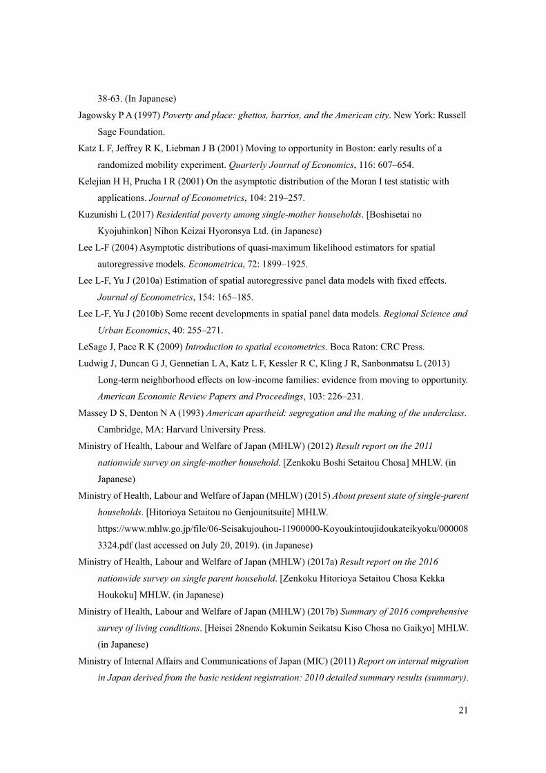
The study area is Japan comprised of 47 prefectures (Figure 1). Those prefectures are broadly

7

categorized into the following nine regions: Hokkaido, Tohoku, Kanto, Chubu, Kansai, Chugoku,

Shikoku, Kyusyu, and Okinawa. The spatial unit of our analysis is a municipality (shi = city; ku =

ward; machi = town; and mura = village), which is the smallest spatial unit with relevant available

data.

In our analysis of children in single-mother households, we use two measures: (1) the

proportion of children under age 6 living in single-mother households and (2) the proportion of

children under age 18 living in single-mother households. Measure (1) is calculated as the number of

children under age 6 in single-mother households divided by the number of children under age 6 in all

households. Similarly, measure (2) is computed as the number of children under age 18 divided by the

number of children under age 18 in all households. We derive these statistics from the published

population data at the municipal level. The number of children in single mother households are

reported for only two age ranges: (1) those less than 6 years old, and (2) those less than 18 years old.

We construct panel data on the two measures at the municipality level. The two measures are

derived from the Population Census of Japan in 2000 and 2010. We use the census, since the

municipal-level analysis requires a sufficient sample size; available survey data have many

municipalities with no observations or only a few. The time for our panel data is limited to two years,

2000 and 2010, since comparable data before 2000 are not available.

Single-mother households in our data are the households that consist of unmarried, widowed,

or divorced mothers and their children and do not include other members such as grandparents. In the

published municipal-level census data of Japan, the numbers of single-mother households that include

members other than mothers and children are available only from 2010. In 2010, the majority (69.9%)

of the single-mother households did not include other members such as grandparents (SBJ, 2017). The

poverty rate of single-mother households without co-residing grandparents is higher than that of

single-mother households with co-residing grandparents (Shirahase and Raymo, 2014; Abe, 2019).12

During 2000–2010, geographic boundaries of some municipalities changed due to municipal

mergers or divisions. In the case of mergers, we aggregated data before mergers into data after

mergers; therefore, the boundaries became those in the latest year, 2010. In the case of divisions, we

aggregate data after divisions into data before division; accordingly, the boundaries are the ones in the

older year, 2000.13 As a result, the total number of municipalities in our sample is 1,852. We created

the municipal boundaries using administrative district data from the National Land Numerical

12 In 2015, the poverty rate of single-mother households without co-residing grandparents is 48.3%, whereas that of single-mother households living with grandparents is 39.8% (Abe, 2019). Shirahase and Raymo (2014) show that the poverty rate of single mothers is reduced if they co-reside with parents. 13 In 2006, Kamikuishiki-mura (a municipality in Yamanashi prefecture) was divided into two already existing different municipalities, a rare style of division. For this particular division, we calculated population-weighted data for each divided portion of the municipality, using the population at the level of blocks (kihontaiku), a spatial unit smaller than municipalities, and then merged the population-weighted data with the data in the existing municipalities.

8

Information download service.

We created panel data on the local income, divorce rate, out-migration rate, and

availability of childcare centers. As a measure of local income, we use average annual income per

person, which we calculate as total taxable annual income divided by the number of taxpayers. The

data are from municipality taxation status and others [Shichoson Kazei Joukyoutou no Shirabe]

available from the Ministry of Internal Affairs and Communications of Japan. For the divorce rate, we

use the refined divorce rate, which is calculated as the number of divorces per 1,000 married women

(England and Kunz, 1975).14 The data on the number of divorces based on the Vital Statistics are from

the Nikkei Electronic Economic Databank System (NIKKEI NEEDS), and the data on the number of

married women come from the Population Census of Japan. The out-migration rate is calculated as the

number of excess out-migration (the number of out-migration subtracted by the number of

in-migration) divided by the population. Data on out-migration, in-migration, and the population

based on the Basic Resident Register are obtained from the NIKKEI NEEDS. The availability of

childcare centers is represented by the ratio of the capacity of licensed childcare centers to the

population of preschool-aged children (under 6 years old). The data are from the Survey of Social

Welfare Institutions and the Population Census. The childcare centers in our data are licensed

childcare centers, which are the major providers of childcare services, offering relatively high quality

and affordable childcare.

4 Methods

4.1 Global and Local Moran’s I

We use Global and Local Moran’s I statistics to examine the spatial clustering patterns of children in

single-mother households. Global Morans I (Moran, 1948, 1950; Cliff and Ord, 1973, 1981) is an

indicator of global spatial autocorrelation. Moran’s I is in essence a cross-product statistic between a

variable and its spatial lag, in which the variable is expressed in deviations from the mean. The Global

Moran’s I value (I) is given by:

I = 𝑛𝑛∑ ∑ 𝑤𝑤𝑖𝑖,𝑗𝑗

𝑛𝑛𝑗𝑗=1

𝑛𝑛𝑖𝑖=1

∑ ∑ 𝑤𝑤𝑖𝑖,𝑗𝑗(𝑦𝑦𝑖𝑖−𝑦𝑦�)(𝑦𝑦𝑗𝑗−𝑦𝑦�)𝑛𝑛𝑗𝑗=1

𝑛𝑛𝑖𝑖=1

∑ (𝑦𝑦𝑖𝑖−𝑦𝑦�)2𝑛𝑛𝑖𝑖=1

, (1)

where n is the number of spatial units (municipalities) indexed by i and j (i ≠j), y is the variable of interest, 𝑦𝑦� is the mean of y, and 𝑤𝑤𝑖𝑖,𝑗𝑗 indicates the spatial weight between i and j. Under the null

hypothesis of no spatial autocorrelation (or spatial randomness), the expected value of Moran’s I and 14 We also experimented with the crude divorce rate (the number of divorces per 1,000 population) and divorce-to-marriage ratio (the number of divorces to the number of marriages). We decided to use the refined divorce rate, which is considered most appropriate among the three measures.

9

the z-score are calculated as follows:

𝐸𝐸[𝐼𝐼] = −1𝑛𝑛−1

, (2)

𝑧𝑧𝐼𝐼 = 𝐼𝐼−𝐸𝐸[𝐼𝐼]�𝑉𝑉[𝐼𝐼]

. (3)

From Eq. (2), we know that the expected value (𝐸𝐸[𝐼𝐼]) is approximately zero when n is large. In this

study, statistical significance is assessed by the pseudo p-value (𝑝𝑝 = 𝑅𝑅+1𝑀𝑀+1

), where R is the number of

times the calculated Moran’s I value from the spatially random data sets (permuted data sets) is equal

to or greater than the observed statistic; M equals the number of permutations (Anselin, 2018). We use

99,999 for the number of permutations. If Moran’s I statistic is significant, a Moran’s I value greater

than 𝐸𝐸[𝐼𝐼] implies spatial clustering (positive spatial autocorrelation, or similar values at neighboring

municipalities), whereas a Moran’s I value less than 𝐸𝐸[𝐼𝐼] indicates spatial dispersion (negative spatial

autocorrelation, or dissimilar values at neighboring municipalities). For the spatial weight matrix, we

use the first-order binary contiguity matrix based on the queen criterion, where two spatial units are

defined as neighbors when they share a common border or vertex. The contiguity matrix is commonly

used for data represented by administrative units that vary in size. We standardize the spatial weight matrix so that each row sums to one. The sum of all the weights (∑ ∑ 𝑤𝑤𝑖𝑖,𝑗𝑗𝑛𝑛

𝑗𝑗=1𝑛𝑛𝑖𝑖=1 ) results in the number

of spatial units (n).

In this study, we present Moran’s I statistics, along with Moran scatter plots (Anselin, 1996,

2018). The Moran scatter plots visualize the original variables on the x-axis, spatially lagged variables

on the y-axis, and the slopes of the linear fit that equal Moran’s I values. The scatter plots are centered

on the mean and comprised four quadrants. The upper-right and lower-left quadrants indicate,

respectively, high-high and low-low spatial autocorrelation (positive spatial autocorrelation). In

contrast, the lower-right and upper-left quadrants denote, respectively, high-low and low-high spatial

autocorrelation (negative spatial autocorrelation). Global Moran’s I statistics and Moran scatter plots

help us detect significant spatial clustering, but they do not identify the locations of significant spatial

clustering within the study area (in Japan).

To discern those locations, we use Local Moran’s I (Anselin, 1995), an indicator of local

spatial autocorrelation. The Local Moran’s I value (𝐼𝐼𝑖𝑖) is computed for each spatial unit i, as follows:

𝐼𝐼𝑖𝑖 = 𝑦𝑦𝑖𝑖−𝑦𝑦�𝑆𝑆𝑖𝑖2 ∑ 𝑤𝑤𝑖𝑖,𝑗𝑗(𝑦𝑦𝑗𝑗 − 𝑦𝑦�)𝑛𝑛

𝑗𝑗=1,j≠i , (4)

where

𝑆𝑆𝑖𝑖2 =∑ (𝑦𝑦𝑗𝑗−𝑦𝑦�)2𝑛𝑛𝑗𝑗=1,𝑗𝑗≠𝑖𝑖

𝑛𝑛−1. (5)

10

The expected value and z-score of Local Moran’s I are computed as:

𝐸𝐸[𝐼𝐼𝑖𝑖] = −∑ 𝑤𝑤𝑖𝑖,𝑗𝑗

𝑛𝑛𝑗𝑗=1,𝑗𝑗≠𝑖𝑖

𝑛𝑛−1, (6)

𝑧𝑧𝐼𝐼𝑖𝑖 = 𝐼𝐼𝑖𝑖−𝐸𝐸[𝐼𝐼𝑖𝑖]�𝑉𝑉[𝐼𝐼𝑖𝑖]

. (7)

As in the case of Global Moran’s I, the queen-based first-order binary contiguity matrix is used

as the spatial weight. A positive 𝐼𝐼𝑖𝑖value indicates that a spatial unit has its neighboring units with

similarly high or low values. In this case, the spatial unit is part of a spatial cluster. A negative 𝐼𝐼𝑖𝑖 value

means that a spatial unit has neighboring units with dissimilar values. In this case, the unit is a spatial

outlier. As in the case of Global Moran’s I, statistical significance is assessed by the pseudo p-value,

which is calculated for each spatial unit, with 99,999 permutations. Based on the 5% significance level

(p < 0.05), we classify significant locations into four types of spatial association: high-high cluster (a

statistically significant spatial cluster of high values), high-low outlier (a statistically significant

spatial outlier with a high value surrounded by low-values), low-high outlier (a statistically significant

spatial outlier with a low value surrounded by high values), and low-low cluster (a statistically

significant spatial cluster of low values). We plot the significant spatial clusters and outliers using

geographic information systems (GIS) to examine their spatial patterns and temporal changes.

4.2 Non-spatial and spatial panel data models

We use panel data models to examine the relationships between the proportions of children in

single-mother households by the age of the children (dependent variables) and local income, the

divorce rates, the out-migration rates, and the availability of childcare centers (explanatory variables).

First, we estimate non-spatial fixed-effects models. The fixed-effects models are selected, since some

omitted municipal characteristics are likely to be correlated with the explanatory variables. Since all of

our explanatory variables are time-variant, their coefficients are identified in the fixed-effects models.

For comparison, we estimate standard models with ordinary least squares (OLS) for pooled data and

non-spatial random-effects models. For an overview of the fixed-effects and random-effects models,

see, for instance, Baltagi (2013) and Wooldridge (2016).

The non-spatial panel data models (for both fixed effects and random effects) are expressed as

follows:

𝑦𝑦𝑖𝑖𝑖𝑖 = α + 𝑋𝑋𝑖𝑖𝑖𝑖𝛽𝛽 + 𝑣𝑣𝑖𝑖 + 𝜖𝜖𝑖𝑖𝑖𝑖 (𝑖𝑖 = 1, … ,𝑁𝑁; 𝑡𝑡 = 1,2, … ,𝑇𝑇), (8)

where i represents units (municipalities), and t indicates time (year). α is a scalar, β is a k × 1 matrix, Xit

11

is a vector of observations for unit i and time t. 𝑣𝑣𝑖𝑖 denotes the unobservable unit-specific error term

that is time-invariant. The fixed-effects models are estimated by using the within regression estimator.

The random-effects models are estimated by using the generalized least squares (GLS) estimator

(producing a matrix-weighted average of the between and within results).

Next, we estimate spatial panel data models, since our municipal-level data are likely to be

spatially autocorrelated. Spatially aggregate units commonly have inherent spatial correlation. The

proportion of children in single-mother households at a location may depend on the proportions at

neighboring locations, and vice versa. The proportions of children in single-mother households may

also depend on the characteristics of neighboring locations. For details on spatial panel data models,

see Baltagi (2013) and Elhorst (2014), among others.

The spatial panel data models are expressed as:

𝑦𝑦𝑛𝑛𝑖𝑖 = λW𝑦𝑦𝑛𝑛𝑖𝑖 + 𝑋𝑋𝑛𝑛𝑖𝑖𝛽𝛽 + 𝑐𝑐𝑛𝑛 + 𝑢𝑢𝑛𝑛𝑖𝑖, (9)

𝑢𝑢𝑛𝑛𝑖𝑖 = 𝜌𝜌M𝑢𝑢𝑛𝑛𝑖𝑖 + v𝑛𝑛𝑖𝑖 (𝑡𝑡 = 1,2, … ,𝑇𝑇),

where ynt = (y1t, y2t,..., ynt)’ represents an n × 1 vector of observations for the dependent variable for

time t with n number of panels; Xnt is an n × k matrix of regressors (including the spatial lags of the

regressors); cn is an n × 1 vector of panel-level effects; unt is an n × 1 vector of the spatially lagged error,

vnt denotes an n × 1 vector of disturbances and is independent and identically distributed (i.i.d.) across

panels and time with variance 𝜎𝜎2 ; and W and M indicate n × n spatial weight matrices. As such, our

spatial models include the spatial lags of the dependent variables, spatially weighted averages of the

regressors, and spatially correlated errors.

Similar to non-spatial panel data models, our preferred specification is the fixed-effects model,

since some omitted municipal characteristics are likely to be correlated with the regressors. The spatial

fixed-effects models are estimated with the quasi-maximum likelihood estimators derived by Lee and

Yu (2010a). For comparison, we estimate spatial random-effects models, in which cn is assumed to be

normal i.i.d. across panels with mean 0 and variance 𝜎𝜎𝑐𝑐2. The random-effects model requires that the

panel-level effects are independent of the observed covariates. The random-effects models are

estimated with the maximum likelihood estimators derived by Lee and Yu (2010b).

For the spatial weight matrices (W and M), we use the first-order binary contiguity matrix

based on the queen criterion, given that characteristics at neighboring municipalities are likely to be

correlated. We experiment with the inverse-distance matrix to investigate whether the results are

sensitive to different weights. The spatial weight matrices are row normalized, so that each row sums

to one.

In both our non-spatial and spatial panel data models, the dependent variable is the proportion

of children in single-mother households by the age of the children. The explanatory variables are the

12

log of average income, or local income (lnINC), the refined divorce rate divided by 100 (RDR/100),

the out-migration rate (OMIGR), and the availability of childcare centers (CHILDC). We divide the

refined divorce rate (RDR) by 100, since the estimated coefficients are too small with the original

RDR. We also include a year dummy (Y2010) and the interactions between the year dummy and the

explanatory variables to examine whether the associations between the proportion of children in

single-mother households and the explanatory variables changed over time.

For each explanatory variable, we present the average marginal effect for the total period

between 2000 and 2010 and each year of 2000 and 2010. In the spatial models, the coefficient

estimates do not represent marginal effects, since the coefficient estimates involve feedback effects

passing through neighboring municipalities and back to the municipalities. Therefore, the average

total, direct, and indirect effects are calculated as the average marginal effects. The total effect is the

sum of the direct and indirect effects (or spillover effect). Each sample excludes municipalities with

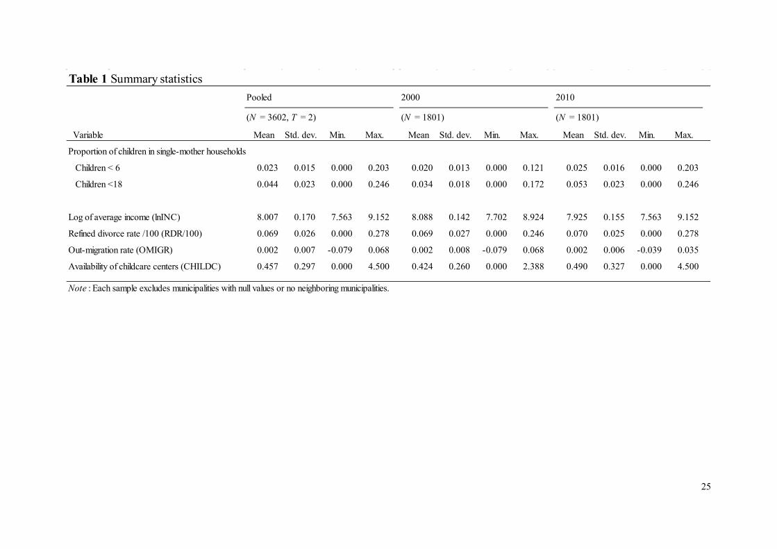
null values or no neighboring municipalities. Our data are balanced panel data. The summary statistics

for the variables in our regression are given in Table 1.

5 Results

5.1 Geographic results

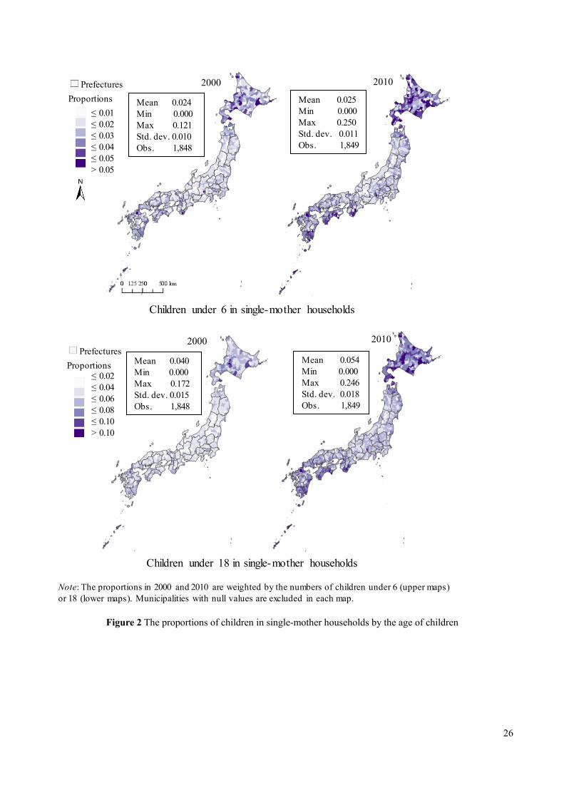
Figure 2 depicts the proportions of children in single-mother households by the age of the children in

2000 and 2010 at the municipal level. Municipalities with null values are excluded in each map. The

summary statistics are presented alongside each map. The choropleth maps reveal three salient

geographic features regarding the children in single-mother households. First, the proportions of

children in single-mother households are not spatially uniform. The average proportion of children

under age 18 in single-mother households was 5.4% in 2010, but there are municipalities where the

value is as low as 0% and as high as 24.6%. Second, the temporal changes in those proportions are also

not spatially uniform. While some municipalities exhibit noticeable increases (particularly in

Hokkaido and western Japan), others show modest decreases or increases (especially in Tohoku and

Chubu regions). Of note, the municipalities with remarkable increases tend to be the municipalities

where the proportions are already high in 2000. Finally, there is spatial clustering; municipalities with

a high proportion of children in single-mother households tend to be geographically close to each

other.

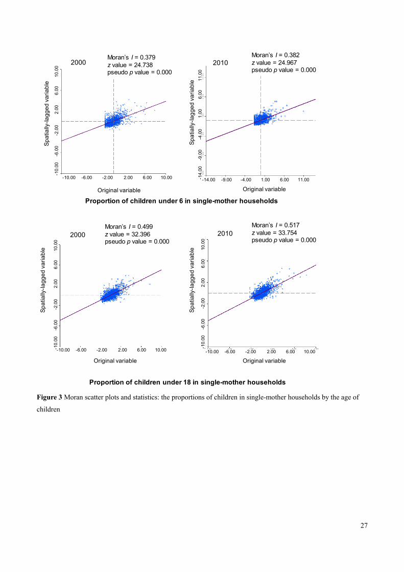
Figure 3 presents the Moran scatter plots of the proportions of children in single-mother

households by the age of the children in 2000 and 2010. The corresponding Global Moran’s I statistics

are shown in the upper center of each scatter plot. The sample excludes municipalities with null values

or no neighboring municipalities (n = 1801). The values in the scatter plots are standardized, and the

units in both axes are in standard deviations (the mean is zero and the standard deviation is one). The

13

scatter plots are presented in square shapes, which is recommended when both axes are measured in

the same units to avoid data distortion (Anselin, 2018). The Moran scatter plots and statistics exhibit

the presence of significant spatial clustering of children in single-mother households. There is a linear relationship between the proportions of children in single-mother households in a

municipality and its neighboring municipalities. The slopes of the fitted lines correspond to Moran’s I

values. Moran’s I values are all highly significant, suggesting a strong rejection of the null hypothesis

(spatial randomness). Positive Moran’s I values indicate that high and low proportions are spatially

clustered, supporting the visualized data in Figure 1.

The Moran scatter plots and statistics reveal two notable trends that are not apparent in the

choropleth maps in Figure 1. First, the intensity of spatial clustering is greater for children under age

18 than for children under age 6. In 2000, the Moran’s I value is 0.499 (z-value = 32.396) for children

under age 18, while it is 0.379 (z-value = 24.738) for children under age 6, suggesting that the older

children are more spatially clustered. Second, from 2000 to 2010, the spatial clustering intensified for

both age groups of children. For children under age 6, the Moran’s I value increases from 0.379

(z-value = 24.738) to 0.382 (z-value = 24.967). For children under age 18, the value grows from 0.499

(z-value=32.396) to 0.517 (z-value = 33.754).15

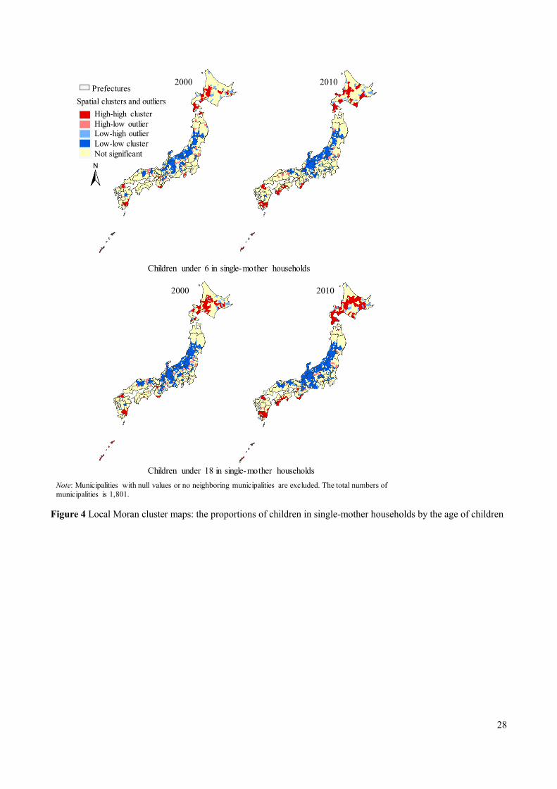
Figure 4 shows the Local Moran cluster maps of the proportions of children in single-mother

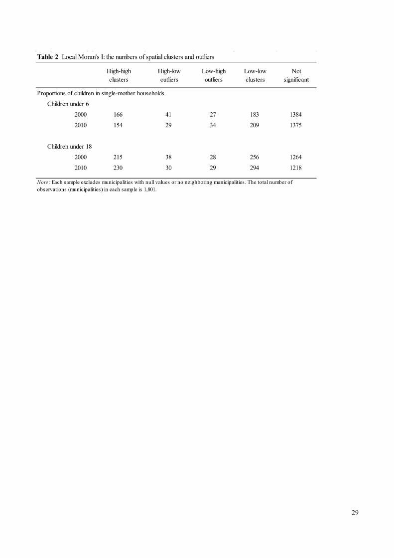
households by the age of the children in 2000 and 2010. Table 2 reports the corresponding numbers of

municipalities that are significant spatial clusters and outliers at the 5% significance level. Each map

excludes municipalities with null values or no neighboring municipalities (n = 1,801). The cluster

maps unveil the presence of a number of spatial clusters and outliers as well as their locations.

High-high clusters represent municipalities with a high proportion of children in single-mother

households surrounded by municipalities with a similarly high proportion. In both 2000 and 2010, the

high-high clusters are located mostly in Hokkaido and western Japan, indicating that children in

single-mother households are spatially clustered in those regions. High-low outliers depict

municipalities with a high proportion of children in single-mother households surrounded by

municipalities with a dissimilarly low proportion. The high-low outliers imply that in these

municipalities, children in single-mother households are concentrated in isolated areas. The numbers

of high-low outliers are relatively small. Most of the high-low outliers are sparsely located in the main

island (Honshu) of Japan.

There are a number of low-low clusters, which depict municipalities with a low proportion

surrounded by municipalities with a similarly low proportion. Many low-low clusters are located in

the Honshu area, indicating that children in single-mother households are relatively rare in those

regions. The numbers of low-high outliers are comparatively small. Notably, low-high outliers are 15 We also calculated differential Moran’s I statistics (Anselin, 2019), or Global Moran’s I statistics for the changes in the proportions of children under ages 6 and 18 in single-mother households from 2000 to 2010. The resultant statistics are significant at the 1% level.

14

located mostly in Hokkaido and western Japan where a number of high-high clusters exist, and many

low-high outliers in those regions are geographically close to the high-high clusters.

The spatial patterns of spatial clusters and outliers for children under age 6 and under age 18

are similar. However, the numbers of spatial clusters are notably greater for children under age 18. In

2010, the number of high-high clusters is 154 for children under age 6, whereas it is 230 for children

under age 18. Similarly, the number of low-low clusters in 2010 is 209 for children under age 6,

whereas it is 294 for children under age 18. The greater numbers of spatial clusters for children under

age 18 align with the larger Global Moran’s I values and their significance for children under age 18

(Figure 2).

The temporal changes from 2000 to 2010 for children under age 6 and those for children under

age 18 show similar spatial patterns. However, the temporal changes in the number of high-high

clusters differ by the age of the children. Whereas the number of high-high clusters decreased for

children under age 6 (from 166 to 154), it increased for children under age 18 (from 215 to 230). This

result suggests that the spatial clustering of children in single-mother households weakened for

children under age 6 but rose for children under age 18. The numbers of low-low clusters, on the other

hand, increased for both age groups, from 183 to 209 for children under age 6 and from 256 to 294 for

children under age 18. Accordingly, the total numbers of high-high and low-low clusters increased for

both age groups, from 349 to 363 for children under age 6 and from 471 to 524 for children under age

18. This result is consistent with the finding from the Global Moran’s I statistics, which indicate the

increased intensity of spatial clustering for both age groups (Figure 2).

For both the children under age 6 and the children under age 18, new high-high clusters tended

to appear in areas geographically close to existing high-high clusters in Hokkaido and western Japan.

In those areas, the high-high clusters extended during the 10-year period. A noticeable number of new

high-high clusters are also found in the Shikoku region, especially in Kochi prefecture (the southern

prefecture in the Shikoku region), in which there were a few high-high clusters in 2000.

5.2 Estimation results

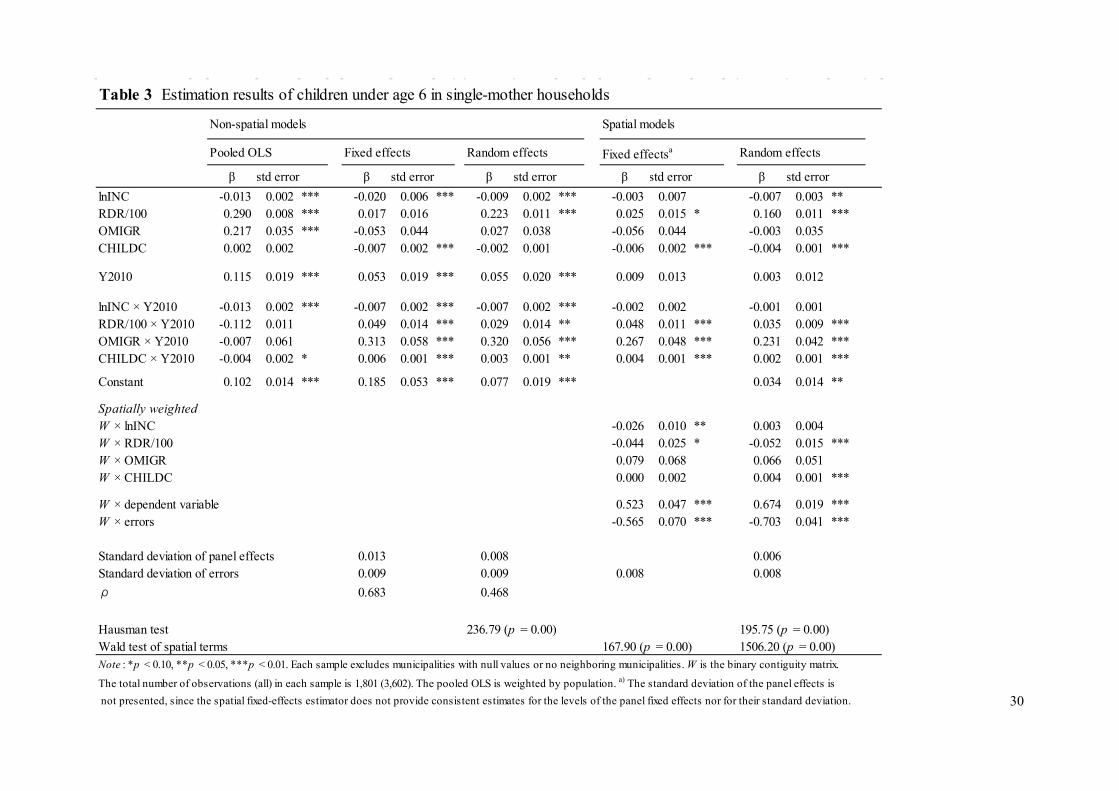
Table 3 shows the estimation results for the proportion of children under age 6 in single-mother

households, from the non-spatial models (pooled OLS, fixed effects, and random effects) and spatial

models (fixed effects and random effects). In both the non-spatial and spatial models, our preferred

specifications are the fixed-effects models. The pooled OLS and random-effects models are presented

for comparison. In both non-spatial and spatial models, the Hausman’s (1978) test statistics are

significant, rejecting the random-effects specifications. The Wald test of the spatial terms indicates

that the additional spatial terms are jointly significant at the 1% level (whether the model is fixed or

random), thereby implying the importance of considering spatial dependency.

Table 4 reports the average marginal effects. The left side shows the average marginal effects

15

of the non-spatial models. We begin by interpreting the results of the non-spatial fixed-effects model

unless otherwise noted. The average marginal effects of local income (lnINC), the refined divorce rate

(RDR/100), the out-migration rate (OMIGR), and the availability of childcare centers (CHILDC) are

all significant. Except for the availability of childcare centers, the signs of the marginal effects are as

we expected and consistent with those in the pooled OLS and random-effects models. The values of

the average marginal effects indicate that a 1% increase in local income is associated with a 0.024

percentage point decrease in the proportion of children under age 6 in single-mother households. An

increase of one divorce per 1,000 married women is associated with a 0.041 percentage point increase

in the proportion of those children. A 1% increase in the out-migration rate is associated with a 0.103

percentage point increase in the proportion of those children. The negative marginal effect of the

availability of childcare centers contradicts our expectation. The results by year show that this

negative marginal effect is significant in 2000 but insignificant in 2010.

The average marginal effects of local income, the divorce rate, and the out-migration rate by

year reveal that their magnitude and significance increased from 2000 to 2010. The magnitude of the

marginal effect of local income increased from -0.020 to -0.027, that of the refined divorce rate

(divided by 100) from 0.017 to 0.066, and that of the out-migration rate from -0.053 to 0.260. In 2010,

the marginal effects of local income, the refined divorce rate, and the out-migration rate are all

significant and their signs agree with our expectations.

Next, we interpret the results based on the spatial fixed-effects model, unless otherwise noted.

The upper part of Table 4 reports the average total, direct, and indirect effects for the period between

2000 and 2010. The total effects of local income, the out-migration rate, and the availability of

childcare centers are significant and greater in magnitude than the average marginal effects in the

non-spatial fixed-effects model. This result suggests that the effects of these variables are larger when

they incorporate both direct and indirect effects (spillover effects). Note that indirect effects are

assumed to be zero in the non-spatial models.

For local income, the direct effect is insignificant, whereas the indirect effect is significant.

The significant and negative indirect effect indicates that, when local income in neighboring

municipalities rises, the proportion of children under age 6 in single-mother households (in their

municipality) falls. The insignificant direct effect is difficult to explain, possibly because the income

level within a municipality is not uniform. Note that the total effect that incorporates both direct and

indirect effects is significant and negative, as expected.

The total effect of the refined divorce rate is insignificant, owing to the insignificant indirect

effect. The direct effect is significant and its value is similar to that in the average marginal effect in the

non-spatial fixed-effects model.16 For the out-migration rate, the total, direct, and indirect effects are

16 The direct effect in the spatial fixed-effects model is 0.00041, and that in the non-spatial fixed-effect model is 0.00047.

16

all significant, and their signs agree with our expectations. The significant and positive direct and

indirect effects suggest that the proportion of children under age 6 in single-mother households

increased in this and neighboring municipalities that experienced a high out-migration rate. For

the availability of childcare centers, the direct effect is significant, whereas the indirect effect is

insignificant. This result suggests that an increase in the proportion of children under age 6 in

single-mother households is significantly associated with a decrease in the availability of childcare

centers in their municipality but is not significantly associated with that in neighboring municipalities.

The lower part of Table 4 presents the total, direct, and indirect effects that are differentiated by

year. One notable change is the out-migration rate. While the total, direct, and indirect effects of the

out-migration rate are insignificant in 2000, they become significant and larger in magnitude in 2010.

In 2010. the total effect of the out-migration rate (0.608) is noticeably greater than the marginal effect

in the non-spatial fixed-effects model (0.260). Given that the direct effect (0.237) has a similar value to

the marginal effect in the non-spatial fixed-effects model (0.260), the larger total effect arises from the

relatively large indirect effect (0.370). Another noteworthy change is that the availability of childcare

centers has significant total and direct effects in 2000, but those effects become insignificant in 2010.

Table 5 reports the estimation results for the proportion of children under age 18 in

single-mother households. In all the non-spatial and spatial models, the coefficients on the year

dummy (Y2010) are positive and significant, suggesting that the proportion of children under age 18

in single-mother households grew from 2000 to 2010, even after controlling for local income, the

refined divorce rate, the out-migration rate, and the availability of childcare centers. The Hausman’s

test statistics are significant in both the non-spatial and spatial models, rejecting the random-effects

specifications. The Wald tests of the spatial terms are highly significant at the 1% level, indicating that

the spatial terms are jointly significant.

Table 6 presents the average marginal effects. We begin with our interpretation of the

non-spatial fixed-effects model. The marginal effects of local income and the out-migration rate are

significant with the expected signs, indicating that a decrease in local income and an increase in the

out-migration rate augments the proportion of children under age 18 in single-mother households.

This result is consistent with that for the pooled OLS and random-effects models. The marginal effect

of the refined divorce rate is insignificant, although it is significant in the pooled OLS and

random-effects models. The availability of childcare centers has a negative and significant marginal

effect, as in the case of the proportion of children under age 6 in single-mother households (Table 4).

The results by year exhibit that the magnitude and significance of the marginal effects of local income,

the refined divorce rate, and the out-migration rate rose from 2000 to 2010. The marginal effect of the

availability of childcare centers lessened its magnitude but continues to be significant. In 2010, all the

marginal effects are significant at the 1% level.

Next, we interpret the results based on the spatial fixed-effects model, unless otherwise noted.

17

The total effects of local income, the refined divorce rate, the out-migration rate, and the availability of

childcare centers are all greater in magnitude than the marginal effects of those variables in the

non-spatial fixed-effect model. This result suggests that the marginal effects are greater when the

model incorporates both direct and indirect effects (spillover effects).

The total effects of local income, the refined divorce rate, the out-migration rate, and the

availability of childcare centers are all significant. The total effect of local income indicates that a 1%

increase in local income is associated with a 0.1 percentage point decrease in the proportion of

children under age 18 in single-mother households. For local income, the direct effect is insignificant,

whereas the indirect effect is significant, as in the case of children under age 6 in single-mother

households (Table 4). The total effect of the refined divorce rate is significant and negative. The direct

effect, however, is positive and significant. The negative total effect, therefore, comes from the

significant and negative indirect effect. This result suggests that an increase in the refined divorce rate

in the municipality augments the proportion of children under age 18 in single-mother households, but

an increase in the refined divorce rate in neighboring municipalities lessens that proportion.

The significant and positive total effect of the out-migration rate implies that a 1% increase in

the out-migration rate is associated with a 0.519 percentage point increase in the proportion of children

under age 18 in single-mother households. For the out-migration rate, the direct and indirect effects are

both significant with expected positive signs. This result suggests that an increase in the out-migration

rate in the municipality as well as in the neighboring municipalities raises the proportion of children

under age 18 in single-mother households. The results by year exhibit that from 2000 to 2010, the

average total, direct, and indirect effects of the out-migration rate all grew in magnitude and

significance, as in the case of the proportion of children under age 6 in single-mother households

(Table 4).

We also estimated the same spatial models using the inverse-distance spatial weight matrix.

The Hausman’s test statistics reject the random-effects specifications, as in the case of the models

using the first-order contiguity matrix. Table A1 summarizes the average total, direct, and indirect

effects in the spatial fixed-effects models. The signs of the significant variables are the same as those

in the models using the first-order contiguity weight. The magnitude of the direct effects is mostly

similar between the two different spatial weights. Notable differences appear in the indirect effects and

resultant total effects. The indirect effects in the models using the inverse-distance spatial weights are

markedly larger in magnitude than those in the models with the first-order contiguity spatial weights.

This result occurs since the inverse-distance weights take into account the effects from not only

neighboring municipalities but also municipalities farther away, although the weights in those distant

municipalities are smaller. Since municipal characteristics are unlikely to be dependent on municipal

characteristics in faraway locations, we prefer the contiguity weights to the inverse-distance weights

in this study. The use of the same contiguity matrix, however, may distort the true spatial relationships,

18

since the spatial relationships are likely to vary by location. The exploration of the appropriate spatial

weights is a topic for future research.

6 Conclusions

Children in single-mother households are not uniformly distributed across municipalities in Japan. As

indicated by Global and Local Moran’s I statistics, there are significant spatial clusters of high

proportions of children in single-mother households (high-high clusters). Those spatial clusters are

located mostly in Hokkaido and western Japan. The spatial clustering patterns for children under age 6

and under age 18 are similar, but the intensity of spatial clustering is notably greater for children under

age 18, with a larger number of high-high clusters. From 2000 to 2010, the number of single-mother

households in Japan increased by 25%. During this 10-year period, the number of high-high clusters

increased for children under age 18 but decreased for children under age 6. These results suggest that

older children in single-mother households are more residentially clustered, and this trend intensified

over the 10-year period.

The total effects in the spatial fixed-effects models indicate that the proportions of children

(both under ages 6 and 18) in single-mother households increased in areas with low income growth,

high out-migration rate, and slow growth in the availability of childcare centers. The negative effect of

local income is in line with the findings that single-mother households are concentrated in low-income

neighborhoods (Winchester, 1990; Jargowsky, 1997). The positive effect of the out-migration rate

suggests that single-mother households might be less likely to move far away from their

neighborhoods. The negative effect of the availability of childcare contradicts our expectation. This

result implies that there is a need for a policy that helps single-mother households access childcare

centers.

The spatial fixed-effects models exhibited the presence of significant indirect effects (spillover

effects). The magnitude of the total effects in the spatial fixed-effects models is greater than that of the

marginal effects in the non-spatial fixed-effects models, suggesting the sizable indirect effects. These

results point to the importance of addressing spatial dependency.

Our findings imply that policies aimed at helping children in single-mother households should

not be uniform across regions. Policy measures to support single-mother households vary by local

government. In Japan, since the enactment of the law to promote measures against child poverty in

2013, various efforts have been made to reduce child poverty. Meanwhile, regional inequality in

anti-child poverty policy efforts has widened in recent years (CAO, 2019). Affluent municipalities

may provide better support, whereas poor municipalities may be unable to provide adequate support.

There may be a geographical mismatch between areas that need more support and areas that offer

better support. Our results can help identify such geographical mismatch as well as critical areas that

19

need further policy attention.

Due to the availability of data, our panel was short—only two years, 2000 and 2010. However,

spatial data are increasingly available. Future research could use spatial panel data that include years

after 2010. In this study, we used the same spatial weights for all municipalities. However, spatial

relationships are likely to differ by location. The exploration of various spatial weights at different

locations is another possibility for further research. Such research using spatial panel data improves

our understanding of the spatial inequality among children in disadvantaged families.

References

Abe A (2019) Trends of child poverty rates: long-term variations from 2012 to 2015. [Kodomo no

Hinkonritsu no Doukou: 2012 kara 2015 to Chokiteki Hendou] Poverty Statistics HP. (in

Japanese)

Allard S W (2017) Places in need: the changing geography of poverty. New York: Russell Sage

Foundation.

Altonji J G, Mansfield R K (2018) Estimating group effects using averages of observables to control

for sorting on unobservables: school and neighborhood effects. American Economic Review, 108

(10): 2902-46.

Anselin L (1995) Local Indicator of Spatial Association-LISA. Geographical Analysis, 6: 93-115.

Anselin L (1996) The Moran scatterplot as an ESDA tool to assess local instability in spatial

association. In Fischer, M., Scholten, H., Unwin, D. (Eds.) Spatial Analytical Perspectives on

GIS (pp. 111–125). London: Taylor & Francis.

Anselin L (2018) Global Spatial Autocorrelation (1): Moran scatter plot and spatial correlogram.

https://geodacenter.github.io/workbook/5a_global_auto/lab5a.html (last accessed Feb. 14,

2019).

Anselin L (2019) Local spatial autocorrelation (2): advanced topics.

https://geodacenter.github.io/workbook/6b_local_adv/lab6b.html (last accessed Feb. 14, 2019).

Anselin L, Rey, S J (2014) Modern spatial econometrics in practice a guide to GeoDa, GeoDaSpace

and PySAL Chikago: GeoDa Press.

Baltagi B H (2013) Econometric analysis of panel data, 5th edition. Chichester, England: John Wiley

& Sons.

Baltagi B H, Liu L (2011) Instrumental variable estimation of a spatial autoregressive panel model

with random effects. Economics Letters, 111: 135–137.

Bartfeld J (2000) Child support and the postdivorce economic well-being of mothers, fathers, and

children. Demography, 37(2): 203-213.

Brooks-Gunn J, Duncan G (1997). The effects of poverty on children. The Future of Children, 7(2),

20

55-71.

Cabinet Office for the Government of Japan (CAO) (2014) General principles regarding measures

against child poverty. [Kodomo no Hinkontaisaku ni Kansuru Taikou ni Tsuite]

https://www8.cao.go.jp/kodomonohinkon/pdf/taikou.pdf (last accessed on July 24, 2019). (in

Japanese).

Cabinet Office for the Government of Japan (CAO) (2019) Suggestions by the panel of experts

regarding policy measures against child poverty (public announcement on august, 2019): about

the ways of future anti-child poverty policy. [Kodomo no Hinkon Taisakuni Kansuru

Yuusikisyakaigi niokeru Teigen (Reiwa Gannen Hachigatsu Kouhyou): Kongo no Kodomo no

Hinkontaisaku no Arikata ni Tsuite]

https://www8.cao.go.jp/kodomonohinkon/yuushikisya/index.html (last accessed on August 9).

(in Japanese).

Chetty R, Hendren N, Katz L F (2016) The effects of exposure to better neighborhoods on children:

new evidence from the moving to opportunity experiment. American Economic Review, 106(4):

855–902.

Chetty R, Hendren N (2018a) The impacts of neighborhoods on intergenerational mobility I:

childhood exposure effects. The Quarterly Journal of Economics, 133: 1107–1162.

Chetty R, Hendren N (2018a) The impacts of neighborhoods on intergenerational mobility II:

county-level estimates. The Quarterly Journal of Economics, 133: 1163–1228.

Chyn E (2018) Moved to opportunity: the long-run effects of public housing demolition on children.

American Economic Review, 108(10): 3028–3056.

Cliff A D, Ord J K (1973) Spatial autocorrelation. London: Pion.

Cliff A D, Ord J K (1981) Spatial processes: models & applications. London: Pion.

Cutler D M, Glaeser E L (1997) Are ghettos good or bad? Quarterly Journal of Economics, 112: 827–

872.

Duncan G, Menestrel S L (eds.) (2019) A roadmap to reducing child poverty. The National Academic

Press.

Elhorst J P (2014) Spatial econometrics: from cross-sectional data to spatial panels. Heidelberg,

Germany: Springer.

England J L, Kunz P R (1975) The application of age-specific rates to divorce. Journal of Marriage

and Family, 37(1): 40-46.

Fageda X, Olivieri C (2019) Transport infrastructure and regional convergence: A spatial panel data

approach. Papers in Regional Science, 98: 1609-1631.

Hausman J A (1978) Specification tests in econometrics. Econometrica, 46: 1251-1271.

Ishii K, Yamada H (2009) Differences in poverty dynamics by age, work and household type in Japan

2005-2007 evidence from Keio household panel survey. Journal of Social Policy Studies, 9:

21

38-63. (In Japanese)

Jagowsky P A (1997) Poverty and place: ghettos, barrios, and the American city. New York: Russell

Sage Foundation.

Katz L F, Jeffrey R K, Liebman J B (2001) Moving to opportunity in Boston: early results of a

randomized mobility experiment. Quarterly Journal of Economics, 116: 607–654.

Kelejian H H, Prucha I R (2001) On the asymptotic distribution of the Moran I test statistic with

applications. Journal of Econometrics, 104: 219–257.

Kuzunishi L (2017) Residential poverty among single-mother households. [Boshisetai no

Kyojuhinkon] Nihon Keizai Hyoronsya Ltd. (in Japanese)

Lee L-F (2004) Asymptotic distributions of quasi-maximum likelihood estimators for spatial

autoregressive models. Econometrica, 72: 1899–1925.

Lee L-F, Yu J (2010a) Estimation of spatial autoregressive panel data models with fixed effects.

Journal of Econometrics, 154: 165–185.

Lee L-F, Yu J (2010b) Some recent developments in spatial panel data models. Regional Science and

Urban Economics, 40: 255–271.

LeSage J, Pace R K (2009) Introduction to spatial econometrics. Boca Raton: CRC Press.

Ludwig J, Duncan G J, Gennetian L A, Katz L F, Kessler R C, Kling J R, Sanbonmatsu L (2013)

Long-term neighborhood effects on low-income families: evidence from moving to opportunity.

American Economic Review Papers and Proceedings, 103: 226–231.

Massey D S, Denton N A (1993) American apartheid: segregation and the making of the underclass.

Cambridge, MA: Harvard University Press.

Ministry of Health, Labour and Welfare of Japan (MHLW) (2012) Result report on the 2011

nationwide survey on single-mother household. [Zenkoku Boshi Setaitou Chosa] MHLW. (in

Japanese)

Ministry of Health, Labour and Welfare of Japan (MHLW) (2015) About present state of single-parent

households. [Hitorioya Setaitou no Genjounitsuite] MHLW.

https://www.mhlw.go.jp/file/06-Seisakujouhou-11900000-Koyoukintoujidoukateikyoku/000008

3324.pdf (last accessed on July 20, 2019). (in Japanese)

Ministry of Health, Labour and Welfare of Japan (MHLW) (2017a) Result report on the 2016

nationwide survey on single parent household. [Zenkoku Hitorioya Setaitou Chosa Kekka

Houkoku] MHLW. (in Japanese)

Ministry of Health, Labour and Welfare of Japan (MHLW) (2017b) Summary of 2016 comprehensive

survey of living conditions. [Heisei 28nendo Kokumin Seikatsu Kiso Chosa no Gaikyo] MHLW.

(in Japanese)

Ministry of Internal Affairs and Communications of Japan (MIC) (2011) Report on internal migration

in Japan derived from the basic resident registration: 2010 detailed summary results (summary).

22

[Juumin Kihon Daicho Jinko Ido Hokoku Heisei 22 Nendo Syousai Syuukei Kekka (Youyaku)]

MIC. https://www.stat.go.jp/data/idou/2010np/shousai/pdf/all.pdf (last accessed on July 20,

2019). (in Japanese)

Moran P A P (1950) Notes on continuous stochastic phenomena. Biometrika, 37(1): 17–23.

Naranpanawa N, Rambaldi A N, Sipe N (2019) Natural amenities and regional tourism employment:

A spatial analysis. Papers in Regional Science, 98: 1731-1757.

Nonoyama-Tarumi Y (2017) Educational achievement of children from single-mother and

single-father families: the case of Japan. Journal of Marriage and Family, 79: 915–931.

Oishi A S (2013) Child support and the poverty of single-mother households in Japan. IPSS

Discussion Paper Series, No.2013-E01.

Oreopoulos P (2003) The long-run consequences of living in a poor neighborhood. Quarterly Journal

of Economics, 118: 1533–1175.

Organisation for Economic Co-operation and Development (OECD) (2011) Doing better for families.

OECD Publishing.

Organisation for Economic Co-operation and Development (OECD) (2016) OECD Family Database:

LMF1.3: Maternal employment by partnership status (updated: 26-09-16).

Organisation for Economic Co-operation and Development (OECD) (2018a) OECD Family Database:

CO2.1: Income inequality and the income position of different household types (updated:

03-01-18).

Organisation for Economic Co-operation and Development (OECD) (2018b) OECD Family

Database: CO2.2: Child poverty (updated: 13-07-18).

Raymo J M, Park H, Iwasawa M, Zhou Y (2014) Single motherhood, living arrangements, and time

with children in Japan. Journal of Marriage and Family, 76: 843–861.

Rowlingson K, McKay S (2002) Lone parent families: gender, class and state. Harlow: Pearson

Education.

Sampson R J (2012) Great American city: Chicago and the enduring neighborhood effect. Chicago:

University of Chicago Press.

Shirahase S, Raymo J M (2014) Single mothers and poverty in Japan: the role of intergenerational

coresidence. Social Forces, 93(2): 545-569.

Skinner C, Bradshaw J, Davidson J (2007) Child support policy: an international perspective.

Research Report No 405, Department for Work and Pensions, University of York.

Statistical Bureau of Japan (SBJ) (2017) 2015 Census: results of basic complete tabulation on

households and families, summary of results. [Heisei 27 Nen Kokusei Chosa: Setai Kouzoutou

Kihon Shukei Kekka, Kekka no Gaiyou] (in Japanese).

Tamiya Y (2019) An analysis of poverty and policy effects towards low wages of single-mother

households. Social Policy, Japan Association for Social Policy Studies, 10(3): 26-38. (in

23

Japanese)

Tamiya Y, Shikata M (2007) Work and childcare in single mother families: a comparative analysis of

mothers time allocation. The Quarterly of Social Security Research, 43(3): 219-231. (in

Japanese)

Thevenon O (2018) Policy brief on child well-being: poor children in rich countries: why we need

policy action. OECD.

Watanabe K, Shikata M (2018) Estimating poverty rates in Japan. [Nihon ni Okeru Hinkonritsu no

Suikei] In Komamura, K. (Ed.) Poverty (pp. 51-62). Minerva Shobo. (in Japanese)

Wilson W J (1987) The truly disadvantaged: the inner city, the underclass, and public policy. Chicago:

The University of Chicago Press.

Winchester H P M (1990) Women and children last: the poverty and marginalization of one-parent

families. Transactions of the Institute of British Geographers, 15(1): 70-86.

Wooldridge J M (2016) Introductory econometrics: a modern approach. 6th edition. Boston:

Cengage.

Zhou Y (2014) Work and life and economic independence of single mothers. [Boshisetai no Work Life

to Keizaitekijiritsu] The Japan Institute for Labour Policy and Training. (in Japanese)

24

Figure 1 Regions, prefectures, and municipalities of Japan

PrefecturesMunicipalities

km

Hokkaido

RegionsPrefectures Tohoku

Kanto

Chubu

KansaiShikoku

Chugoku

Kyushu

Okinawa

Tokyo

Osaka

Hokkaido

Okinawa

25

Table 1 Summary statisticsPooled 2000 2010

(N = 3602, T = 2) (N = 1801) (N = 1801)

Variable Mean Std. dev. Min. Max. Mean Std. dev. Min. Max. Mean Std. dev. Min. Max.

Proportion of children in single-mother households

Children < 6 0.023 0.015 0.000 0.203 0.020 0.013 0.000 0.121 0.025 0.016 0.000 0.203

Children <18 0.044 0.023 0.000 0.246 0.034 0.018 0.000 0.172 0.053 0.023 0.000 0.246

Log of average income (lnINC) 8.007 0.170 7.563 9.152 8.088 0.142 7.702 8.924 7.925 0.155 7.563 9.152

Refined divorce rate /100 (RDR/100) 0.069 0.026 0.000 0.278 0.069 0.027 0.000 0.246 0.070 0.025 0.000 0.278

Out-migration rate (OMIGR) 0.002 0.007 -0.079 0.068 0.002 0.008 -0.079 0.068 0.002 0.006 -0.039 0.035

Availability of childcare centers (CHILDC) 0.457 0.297 0.000 4.500 0.424 0.260 0.000 2.388 0.490 0.327 0.000 4.500

Note : Each sample excludes municipalities with null values or no neighboring municipalities.

26

Figure 2 The proportions of children in single-mother households by the age of children

Children under 18 in single-mother households

PrefecturesProportions

≤ 0.01≤ 0.02≤ 0.03≤ 0.04≤ 0.05> 0.05

Children under 6 in single-mother households

PrefecturesProportions

≤ 0.02≤ 0.04≤ 0.06≤ 0.08≤ 0.10> 0.10

Mean 0.024 Min 0.000Max 0.121Std. dev. 0.010Obs. 1,848

Mean 0.025 Min 0.000Max 0.250Std. dev. 0.011Obs. 1,849

Mean 0.040 Min 0.000Max 0.172Std. dev. 0.015Obs. 1,848

Mean 0.054 Min 0.000Max 0.246Std. dev. 0.018Obs. 1,849

20102000

20102000

Note: The proportions in 2000 and 2010 are weighted by the numbers of children under 6 (upper maps) or 18 (lower maps). Municipalities with null values are excluded in each map.

27

Figure 3 Moran scatter plots and statistics: the proportions of children in single-mother households by the age of

children

Proportion of children under 18 in single-mother households

Proportion of children under 6 in single-mother households

Spat

ially

-lagg

ed v

aria

ble

20102000Moran’s I = 0.517z value = 33.754pseudo p value = 0.000

Moran’s I = 0.499z value = 32.396pseudo p value = 0.000

Moran’s I = 0.382z value = 24.967pseudo p value = 0.000

Original variable

-10.00 -6.00 -2.00 2.00 6.00 10.00 -10.

00

-6.

00

-

2.00

2.

00

6

.00

10.0

0

20102000

-10.00 -6.00 -2.00 2.00 6.00 10.00

-10.

00

-6.

00

-

2.00

2.

00

6

.00

10.0

0

-14.00 -9.00 -4.00 1.00 6.00 11.00 -14.

00

-9.

00

-

4.00

1.

00

6

.00

11.0

0

Moran’s I = 0.379z value = 24.738pseudo p value = 0.000

Spat

ially

-lagg

ed v

aria

ble

Original variable

Spat

ially

-lagg

ed v

aria

ble

Original variable

-10.00 -6.00 -2.00 2.00 6.00 10.00 -10.00 -6.00 -2.00 2.00 6.00 10.00 -10.00 -6.00 -2.00 2.00 6.00 10.00

-10.

00

-6.

00

-

2.00

2.

00

6

.00

10.0

0

Spat

ially

-lagg

ed v

aria

ble

Original variable

28

Figure 4 Local Moran cluster maps: the proportions of children in single-mother households by the age of children

Children under 18 in single-mother households

Children under 6 in single-mother households

PrefecturesSpatial clusters and outliers

20102000

20102000

High-high clusterHigh-low outlierLow-high outlierLow-low clusterNot significant

Note: Municipalities with null values or no neighboring municipalities are excluded. The total numbers of municipalities is 1,801.

29

Table 2 Local Moran's I: the numbers of spatial clusters and outliers

High-highclusters

High-lowoutliers

Low-highoutliers

Low-lowclusters

Notsignificant

Proportions of children in single-mother households

Children under 6

2000 166 41 27 183 1384

2010 154 29 34 209 1375

Children under 18

2000 215 38 28 256 1264

2010 230 30 29 294 1218

Note : Each sample excludes municipalities with null values or no neighboring municipalities. The total number ofobservations (municipalities) in each sample is 1,801.

30

Table 3 Estimation results of children under age 6 in single-mother households

Non-spatial models Spatial models

Pooled OLS Fixed effects Random effects Fixed effectsa Random effects

β std error β std error β std error β std error β std errorlnINC -0.013 0.002 *** -0.020 0.006 *** -0.009 0.002 *** -0.003 0.007 -0.007 0.003 **RDR/100 0.290 0.008 *** 0.017 0.016 0.223 0.011 *** 0.025 0.015 * 0.160 0.011 ***OMIGR 0.217 0.035 *** -0.053 0.044 0.027 0.038 -0.056 0.044 -0.003 0.035CHILDC 0.002 0.002 -0.007 0.002 *** -0.002 0.001 -0.006 0.002 *** -0.004 0.001 ***

Y2010 0.115 0.019 *** 0.053 0.019 *** 0.055 0.020 *** 0.009 0.013 0.003 0.012

lnINC × Y2010 -0.013 0.002 *** -0.007 0.002 *** -0.007 0.002 *** -0.002 0.002 -0.001 0.001RDR/100 × Y2010 -0.112 0.011 0.049 0.014 *** 0.029 0.014 ** 0.048 0.011 *** 0.035 0.009 ***OMIGR × Y2010 -0.007 0.061 0.313 0.058 *** 0.320 0.056 *** 0.267 0.048 *** 0.231 0.042 ***CHILDC × Y2010 -0.004 0.002 * 0.006 0.001 *** 0.003 0.001 ** 0.004 0.001 *** 0.002 0.001 ***

Constant 0.102 0.014 *** 0.185 0.053 *** 0.077 0.019 *** 0.034 0.014 **

Spatially weightedW × lnINC -0.026 0.010 ** 0.003 0.004W × RDR/100 -0.044 0.025 * -0.052 0.015 ***W × OMIGR 0.079 0.068 0.066 0.051W × CHILDC 0.000 0.002 0.004 0.001 ***

W × dependent variable 0.523 0.047 *** 0.674 0.019 ***W × errors -0.565 0.070 *** -0.703 0.041 ***

Standard deviation of panel effects 0.013 0.008 0.006Standard deviation of errors 0.009 0.009 0.008 0.008ρ 0.683 0.468

Hausman test 236.79 (p = 0.00) 195.75 (p = 0.00)Wald test of spatial terms 167.90 (p = 0.00) 1506.20 (p = 0.00)Note : *p < 0.10, **p < 0.05, ***p < 0.01. Each sample excludes municipalities with null values or no neighboring municipalities. W is the binary contiguity matrix.

The total number of observations (all) in each sample is 1,801 (3,602). The pooled OLS is weighted by population. a) The standard deviation of the panel effects is not presented, since the spatial fixed-effects estimator does not provide consistent estimates for the levels of the panel fixed effects nor for their standard deviation.

31

Table 4 Average marginal effects for children under age 6 in single-mother householdsNon-spatial models Spatial models: fixed effects Spatial models: random effects

Pooled OLS Fixed effects Rondom effects Total Direct Indirect Total Direct Indirect

2000-2010lnINC -0.019 *** -0.024 *** -0.012 *** -0.062 *** -0.008 -0.054 *** -0.014 *** -0.008 *** -0.006

(0.001) (0.006) (0.002) (0.013) (0.007) (0.014) (0.005) (0.003) (0.005)RDR/100 0.236 *** 0.041 *** 0.237 *** 0.011 0.047 *** -0.036 0.385 *** 0.192 *** 0.193 ***

(0.006) (0.014) (0.009) (0.044) (0.014) (0.042) (0.032) (0.010) (0.030)OMIGR 0.214 *** 0.103 ** 0.187 *** 0.328 *** 0.094 ** 0.234 ** 0.547 *** 0.144 *** 0.403 ***

(0.030) (0.040) (0.032) (0.124) (0.040) (0.118) (0.126) (0.031) (0.119)CHILDC 0.000 -0.004 *** 0.000 -0.008 * -0.004 *** -0.004 0.004 -0.002 *** 0.006 **

(0.001) (0.001) (0.001) (0.005) (0.001) (0.004) (0.003) (0.001) (0.003)By year

2000lnINC -0.013 *** -0.020 *** -0.009 *** -0.060 *** -0.007 -0.053 *** -0.013 ** -0.008 *** -0.005

(0.002) (0.006) (0.002) (0.013) (0.007) (0.014) (0.005) (0.003) (0.006)RDR/100 0.290 *** 0.017 0.223 *** -0.039 0.021 -0.060 0.332 *** 0.172 *** 0.160 ***

(0.008) (0.016) (0.011) (0.044) (0.015) (0.042) (0.033) (0.011) (0.030)OMIGR 0.217 *** -0.053 0.027 0.048 -0.049 0.097 0.193 0.011 0.182

(0.035) (0.044) (0.038) (0.120) (0.043) (0.115) (0.127) (0.035) (0.118)CHILDC 0.002 -0.007 *** -0.002 -0.012 ** -0.006 *** -0.006 0.000 -0.004 *** 0.004

(0.002) (0.002) (0.001) (0.005) (0.002) (0.004) (0.004) (0.001) (0.003)2010

lnINC -0.026 *** -0.027 *** -0.016 *** -0.065 *** -0.009 -0.055 *** -0.016 *** -0.009 *** -0.007(0.002) (0.006) (0.002) (0.013) (0.007) (0.014) (0.005) (0.003) (0.006)

RDR/100 0.178 *** 0.066 *** 0.252 *** 0.061 0.072 *** -0.012 0.438 *** 0.212 *** 0.226 ***(0.008) (0.016) (0.012) (0.047) (0.015) (0.043) (0.036) (0.011) (0.032)

OMIGR 0.210 *** 0.260 *** 0.347 *** 0.608 *** 0.237 *** 0.370 *** 0.901 *** 0.276 *** 0.625 ***(0.050) (0.054) (0.047) (0.147) (0.051) (0.129) (0.154) (0.043) (0.134)

CHILDC -0.002 -0.001 0.001 -0.003 -0.001 -0.002 0.008 ** -0.001 0.009 ***(0.002) (0.001) (0.001) (0.004) (0.001) (0.004) (0.003) (0.001) (0.003)

Note : Standard errors are in parentheses. *p < 0.10, **p < 0.05, ***p < 0.01.

32

Table 5 Estimation results of children under age 18 in single-mother households

Non-spatial models Spatial models

Pooled OLS Fixed effects Random effects Fixed effectsa Random effects

β std error β std error β std error β std error β std errorlnINC -0.012 0.003 *** -0.020 0.006 *** -0.003 0.003 0.003 0.007 0.006 0.004RDR/100 0.488 0.013 *** -0.042 0.015 *** 0.214 0.013 *** -0.006 0.014 0.158 0.013 ***OMIGR 0.376 0.057 *** -0.001 0.044 0.049 0.043 0.000 0.040 0.043 0.037CHILDC 0.004 0.002 -0.007 0.002 *** -0.004 0.002 *** -0.005 0.002 *** -0.007 0.001 ***

Y2010 0.282 0.031 *** 0.179 0.019 *** 0.167 0.021 *** 0.056 0.013 *** 0.041 0.012 ***

lnINC × Y2010 -0.031 0.004 *** -0.022 0.002 *** -0.020 0.003 *** -0.008 0.002 *** -0.005 0.001 ***RDR/100 × Y2010 -0.161 0.018 *** 0.114 0.014 *** 0.089 0.015 *** 0.074 0.010 *** 0.057 0.009 ***OMIGR × Y2010 0.024 0.099 0.354 0.058 *** 0.405 0.061 *** 0.234 0.044 *** 0.240 0.042 ***CHILDC × Y2010 -0.010 0.003 *** 0.003 0.001 ** 0.000 0.001 0.001 0.001 0.001 0.001

Constant 0.098 0.022 *** 0.202 0.052 *** 0.048 0.025 ** 0.032 0.019 *

Spatially weightedW × lnINC -0.031 0.009 *** -0.009 0.004 **W × RDR/100 -0.063 0.023 *** -0.087 0.018 ***W × OMIGR 0.052 0.063 -0.009 0.055W × CHILDC -0.001 0.002 0.006 0.002 ***

W × dependent variable 0.675 0.030 *** 0.742 0.015 ***W × errors -0.581 0.061 *** -0.668 0.047 ***

Standard deviation of panel effects 0.020 0.013 0.010Standard deviation of errors 0.009 0.009 0.007 0.008ρ 0.840 0.699

Hausman test 1240.12 (p = 0.00) 1057.59 (p = 0.00)Wald test of spatial terms 767.07 (p = 0.00) 2968.49 (p = 0.00)Note : *p < 0.10, **p < 0.05, ***p < 0.01. Each sample excludes municipalities with null values or no neighboring municipalities. W is the binary contiguity matrix.

The total number of observations (all) in each sample is 1,801 (3,602). The pooled OLS is weighted by population. a) The standard deviation of the panel effects is not presented, since the spatial fixed-effects estimator does not provide consistent estimates for the levels of the panel fixed effects nor for their standard deviation.

33

Table 6 Average marginal effects for children under age 18 in single-mother householdsNon-spatial models Spatial models: fixed effects Spatial models: random effects

Pooled OLS Fixed effects Rondom effects Total Direct Indirect Total Direct Indirect

2000-2010lnINC -0.027 *** -0.031 *** -0.013 *** -0.100 *** -0.008 -0.091 *** -0.023 *** 0.001 -0.024 ***

(0.002) (0.006) (0.003) (0.017) (0.006) (0.017) (0.009) (0.004) (0.009)RDR/100 0.411 *** 0.015 0.259 *** -0.098 * 0.022 * -0.120 ** 0.387 *** 0.201 *** 0.186 ***

(0.009) (0.014) (0.012) (0.059) (0.013) (0.055) (0.052) (0.012) (0.048)OMIGR 0.388 *** 0.176 *** 0.252 *** 0.519 *** 0.145 *** 0.373 ** 0.595 *** 0.193 *** 0.402 **

(0.049) (0.040) (0.038) (0.164) (0.038) (0.154) (0.178) (0.035) (0.166)CHILDC -0.001 -0.006 *** -0.005 *** -0.014 ** -0.005 *** -0.009 * -0.004 -0.007 *** 0.003

(0.002) (0.001) (0.001) (0.006) (0.001) (0.006) (0.005) (0.001) (0.005)By year

2000lnINC -0.012 *** -0.020 *** -0.003 -0.088 *** -0.004 -0.084 *** -0.013 0.004 -0.017 *

(0.003) (0.006) (0.003) (0.018) (0.007) (0.018) (0.009) (0.004) (0.009)RDR/100 0.488 *** -0.042 *** 0.214 *** -0.211 *** -0.020 -0.191 *** 0.276 *** 0.166 *** 0.109 **

(0.013) (0.015) (0.013) (0.059) (0.014) (0.055) (0.053) (0.013) (0.048)OMIGR 0.376 *** -0.001 0.049 0.159 0.011 0.148 0.131 0.049 0.082

(0.057) (0.044) (0.043) (0.160) (0.040) (0.149) (0.177) (0.038) (0.164)CHILDC 0.004 -0.007 *** -0.004 *** -0.016 ** -0.006 *** -0.011 * -0.005 -0.007 *** 0.002

(0.002) (0.002) (0.002) (0.006) (0.002) (0.006) (0.006) (0.001) (0.005)2010

lnINC -0.044 *** -0.042 *** -0.023 *** -0.111 *** -0.013 ** -0.099 *** -0.033 *** -0.002 -0.031 ***(0.003) (0.006) (0.003) (0.017) (0.006) (0.017) (0.009) (0.004) (0.009)

RDR/100 0.326 *** 0.072 *** 0.303 *** 0.015 0.064 *** -0.049 0.497 *** 0.235 *** 0.262 ***(0.013) (0.016) (0.014) (0.062) (0.015) (0.057) (0.057) (0.014) (0.051)

OMIGR 0.401 *** 0.353 *** 0.454 *** 0.878 *** 0.280 *** 0.599 *** 1.060 *** 0.337 *** 0.722 ***(0.081) (0.054) (0.054) (0.195) (0.049) (0.171) (0.214) (0.047) (0.187)

CHILDC -0.006 ** -0.004 *** -0.005 *** -0.012 ** -0.004 *** -0.008 -0.003 -0.006 *** 0.004(0.002) (0.001) (0.001) (0.006) (0.001) (0.006) (0.005) (0.001) (0.005)

Note : Standard errors are in parentheses. *p < 0.10, **p < 0.05, ***p < 0.01.

34

Table A1 Average marginal effects for children under ages 6 and 18 in single-mother households: spatial fixed-effects models

Children under age 6 Children under age 18

Total Direct Indirect Total Direct Indirect

2000-2010lnINC -0.553 ** -0.010 -0.544 ** -0.772 *** -0.010 -0.761 ***

(0.252) (0.007) (0.253) (0.272) (0.006) (0.272)RDR/100 -0.874 0.047 *** -0.921 -1.056 0.021 -1.076

(0.668) (0.014) (0.667) (0.775) (0.013) (0.773)OMIGR 3.765 0.081 ** 3.683 3.216 0.131 *** 3.085

(2.323) (0.040) (2.321) (2.047) (0.037) (2.040)CHILDC -0.033 -0.004 ** -0.030 0.033 -0.003 ** 0.036

(0.057) (0.001) (0.057) (0.091) (0.001) (0.090)By year

2000lnINC -0.551 ** -0.008 -0.542 ** -0.755 *** -0.002 -0.753 ***

(0.252) (0.007) (0.252) (0.268) (0.007) (0.267)RDR/100 -0.923 0.021 -0.944 -1.157 -0.032 ** -1.125

(0.683) (0.0157) (0.683) (0.794) (0.015) (0.792)OMIGR 3.519 -0.049 3.567 3.090 0.066 3.024

(2.224) (0.044) (2.223) (2.017) (0.042) (2.012)CHILDC -0.039 -0.007 *** -0.032 0.032 -0.004 ** 0.036

(0.057) (0.002) (0.057) (0.091) (0.002) (0.090)2010

lnINC -0.556 ** -0.011 * -0.545 ** -0.788 *** -0.019 *** -0.769 ***(0.253) (0.007) (0.253) (0.277) (0.006) (0.277)

RDR/100 -0.825 0.072 *** -0.898 -0.954 0.073 *** -1.027(0.654) (0.016) (0.652) (0.759) (0.015) (0.755)

OMIGR 4.011 * 0.211 *** 3.800 3.342 0.196 *** 3.146(2.426) (0.054) (2.422) (2.079) (0.052) (2.069)

CHILDC -0.028 -0.001 -0.027 0.034 -0.003 ** 0.037(0.057) (0.001) (0.057) (0.091) (0.001) (0.091)

Note : Standard errors are in parentheses. *p < 0.10, **p < 0.05, ***p < 0.01.