Nonlinear Finite Element Method

04/10/2004

Nonlinear Finite Element Method

• Lectures include discussion of the nonlinear finite element method.• It is preferable to have completed “Introduction to Nonlinear Finite Element Analysis”

available in summer session.• If not, students are required to study on their own before participating this course.

Reference:Toshiaki.,Kubo. “Introduction: Tensor Analysis For Nonlinear Finite Element Method” (Hisennkei Yugen Yoso no tameno Tensor Kaiseki no Kiso),Maruzen.

• Lecture references are available and downloadable athttp://www.sml.k.utokyo.ac.jp/members/nabe/lecture2004 They should be put up on the website by the day before scheduled meeting day, and each students are expected to come in with a copy of the reference.

•Lecture notes from previous year are available and downloadable, also at http://www.sml.k.u.tokyo.ac.jp/members/nabe/lecture2003 You may find the course title, ”Advanced Finite Element Method” but the contents covered are almost the same I will cover this year.

• I will assign the exercises from this year, and expect the students to hand them in during the following lecture. They are not the requirements and they will not be graded, however it is important to actually practice calculate in deeper understanding the finite element method.

• For any questions, contact me at nabe@sml.k.u-tokyo.ac.jp

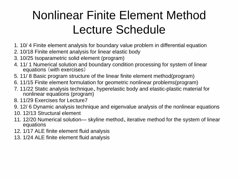
Nonlinear Finite Element Method Lecture Schedule

1. 10/ 4 Finite element analysis for boundary value problem in differential equation2. 10/18 Finite element analysis for linear elastic body3. 10/25 Isoparametric solid element (program)4. 11/ 1 Numerical solution and boundary condition processing for system of linear

equations （with exercises）5. 11/ 8 Basic program structure of the linear finite element method(program)6. 11/15 Finite element formulation for geometric nonlinear problems(program)7. 11/22 Static analysis technique、hyperelastic body and elastic-plastic material for

nonlinear equations (program)8. 11/29 Exercises for Lecture79. 12/ 6 Dynamic analysis technique and eigenvalue analysis of the nonlinear equations10. 12/13 Structural element11. 12/20 Numerical solution— skyline method、iterative method for the system of linear

equations12. 1/17 ALE finite element fluid analysis13. 1/24 ALE finite element fluid analysis

Review on the Finite Element Method— For Typical Numerical Solutions

• In physics, various phenomenon are interpreted in mathematical representations (differential equations, for example, are used in Newtonian mechanics).

• Finite element analysis is an approximate analysis for differential equations

• Finite difference calculus:– Directly discretize the governing equations, and is theoretically simple,

and it is easy to program.– Which is met for Euler representation, however, not suitable for

Lagrange representation.• Finite element method:– Discretize the governing equation in weak formulation– Common analysis for solid・structural problems and fluid– Programming is complicated

Boundary Value Problems in Differential Equations

• Consider the boundary value problems in differential equations.Obtain u that satisfies the conditions for [B]

•If f(x) is concerned with the problems that are analytically integrable, the solution u can be obtained by direct integration.

• Finite element method involves with approximate analysis of the weak form of the differential equations. The processes of obtaining the approximate solution are:

– Weak formulation of the differential equations.– Eliminate the finite element interpolation function to substitute the continuous

functions into the discrete nodal point value.– Based on the above, construct the system of linear equations to obtain the

approximate solution.

Strong Form and Weak Form

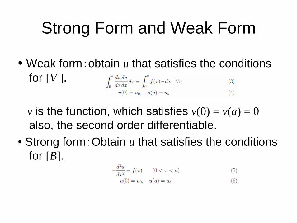
• Weak form：obtain u that satisfies the conditions for [V ].

v is the function, which satisfies v(0) = v(a) = 0also, the second order differentiable.

• Strong form：Obtain u that satisfies the conditions for [B].

Deriving the Weak Formulation of the Differential Equations 1

• Given the differential equation:

Multiply the the second-order differentiable function v, which satisfies the condition v(0) = v(a) = 0, on both sides then conduct integration of domain(0to a).

• Integrate the left hand side equation in the above by parts.

So,

Given that,

Deriving the Weak Formulation of the Differential Equations 2

• Given, v(0) = v(a) = 0 the second term in the left hand side becomes 0

• Thus

• By satisfying the boundary condition v(0) = v(a) = 0, we can also establish for the arbitrary v. Hence, [V ] is proofed from [B].

Deriving the Weak Formulation of the Differential Equations 3

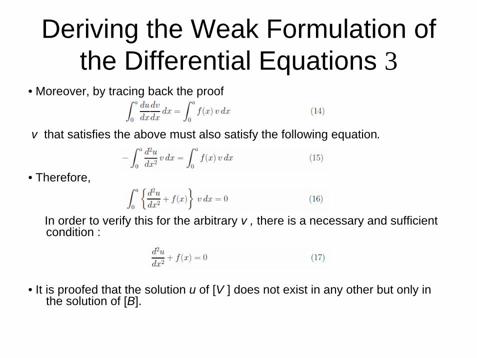
• Moreover, by tracing back the proof

v that satisfies the above must also satisfy the following equation.

• Therefore,

In order to verify this for the arbitrary v , there is a necessary and sufficient condition :

• It is proofed that the solution u of [V ] does not exist in any other but only in the solution of [B].

Strong Form and Weak Form

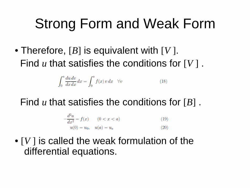
• Therefore, [B] is equivalent with [V ].Find u that satisfies the conditions for [V ] .

Find u that satisfies the conditions for [B] .

• [V ] is called the weak formulation of the differential equations.

Weak Form and the Minimization Problems 1

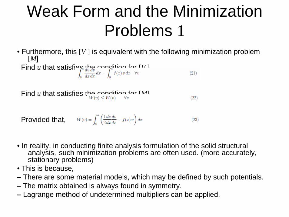
• Furthermore, this [V ] is equivalent with the following minimization problem [M]

Find u that satisfies the condition for [V ].

Find u that satisfies the condition for [M]

Provided that,

• In reality, in conducting finite analysis formulation of the solid structural analysis，such minimization problems are often used. (more accurately, stationary problems)

• This is because,– There are some material models, which may be defined by such potentials.– The matrix obtained is always found in symmetry.– Lagrange method of undetermined multipliers can be applied.

Weak Form and the Minimization Problems 2

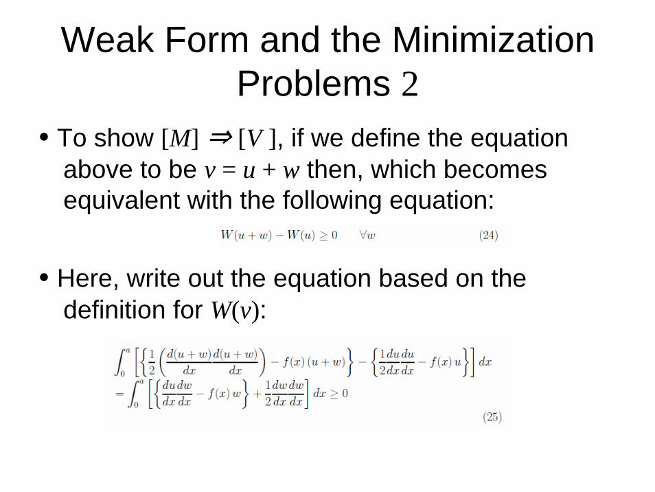
• To show [M] ⇒ [V ], if we define the equation above to be v = u + w then, which becomes equivalent with the following equation:

• Here, write out the equation based on the definition for W(v):

Weak Form and the Minimization Problems 3

• This equation must be also established for the arbitrary w, thus we define α as the arbitrary scalar to substituteαw into w. To put it in order:

•Where ,the left hand side becomes 0 thus it is established.

•Where ,we consider it as the quadratic equations of α．

• Therefore,

Weak Form and the Minimization Problems 4

• A necessary and sufficient condition for y ≥ 0 is where a >0 and b2− 4ac ≤ 0 (discriminant),however in this case the condition may be b = 0

•In other words，

•Thus, [V ] should be proofed by [M].• For [V ] ⇒ [M], we can make a proof by having a

definition W(u+w)−W(u) to calculate then gain the following:

Approximate Solutions for Weak Form—Dividing the Interval of Integrations

• Obtain the approximate solution for the weak form by the finite element method.

• First, divide the domain [0, a] of u into the n intervals of [xi, xi+1] (i = 1～n) where there is no overlapping of u.

• This xi (i = 1 ～ n + 1) is called a nodal point.• Now the integration of can be reformed as the

following.

• We assume the approximate solution to take the value ui (i = 1 ～ n + 1) in the nodal point xi (i = 1 ～ n + 1), and where in between the nodal points xi and xi+1, we assume the solution takes changes linearly. In this case, we use the similar functions of v.

Finite Element Method Interpolation1

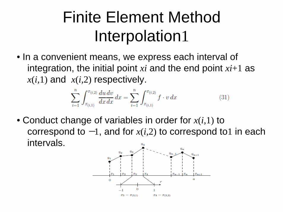
• In a convenient means, we express each interval of integration, the initial point xi and the end point xi+1 as x(i,1) and x(i,2) respectively.

• Conduct change of variables in order for x(i,1) to correspond to −1, and for x(i,2) to correspond to1 in each intervals.

Finite Element Method Interpolation2

• Now,using the parameter r (−1 ≤ r ≤ 1), x found in [x(i,1),x(i,2)] can be expressed in the following form.

• N(i) is called the finite element method interpolation function, or simply the interpolation function.

Finite Element Method Interpolation3

• Likewise, for , using the parameter r (−1 ≤ r ≤ 1) to express in the following form.

Only where,

Discrete Value Expression of Differentiation

• Substitute the weak form into the approximate solution to obtain the following:

In the left hand side, the derivative of the function x of in the integrand can be obtained by using the chain rule.

•For appears in the equation above, the inverse numbers may be obtained. In actual programming,

We obtain in the beginning then substitute it into the above equation to follow the calculations shows in below:

Element Matrix1

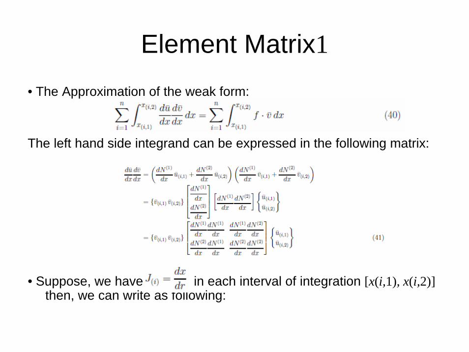
• The Approximation of the weak form:

The left hand side integrand can be expressed in the following matrix:

• Suppose, we have in each interval of integration [x(i,1), x(i,2)]then, we can write as following:

• The following equation may be obtained with this tedious work of writing out the matrix. It is important to realize dx/dr and dr/dx are used in a different meaning.

Element Matrix 2• are the values in the nodal points，and remain constant in terms

of r, the variable of integration, therefore we may leave them out of the integrals.

• [K(i)], which defines {F(i)} in the following equation, is called the element matrix.

Compound Matrix1

• Write out the both sides of the equation without using Σ.

• Therefore,

Compound Matrix2

• Whereas, we can force to write in the matrix representation shows in the following:

• The second matrix may be written as:

Compound Matrix3

• In the same way, for the ith matrix, we can generalize to write as the following:

• Based on the above，

Compound Matrix4• The n + 1 × n + 1 dimensional matrix [K] made by superposition of the element matrix is

called the compound matrix.

• The component of {F} can be written as.

• Using this matrix notation in the above, the following equation (56)can be written as (57)

.

Compound Matrix5• The following condition is required for the arbitrary v

However, the condition above is established only when,

• Hence the approximate solution is required for the weak form of the differential equations as the system of linear equations shows in the following,

• These are the basic procedures of the finite element method.

Discretization Error of the Finite Element Method

• Finite element method is the approximate solution of the differential equations.

• While the solutions of the differential equations are continuous, the solutions of the finite element method are found within the range of unknown numbers.

• Essentially, involves the errors• Which is called the discretization error• Does error decrease in accordance with the finite

element partitions becoming smaller?

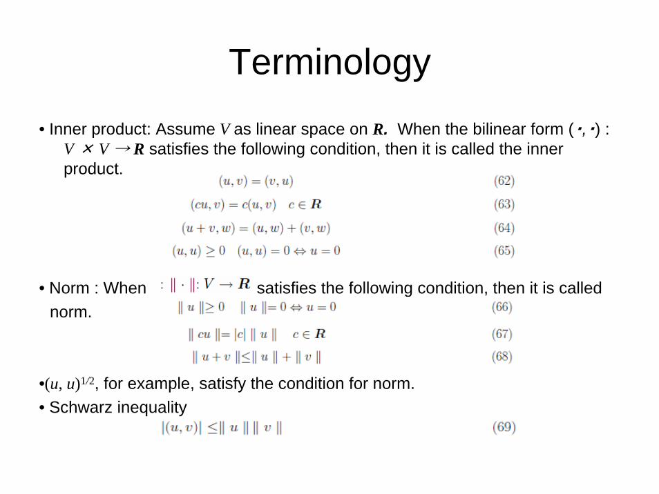
Terminology• Inner product: Assume V as linear space on R. When the bilinear form (・,・) :

V × V → R satisfies the following condition, then it is called the inner product.

• Norm : When satisfies the following condition, then it is called norm.

•(u, u)1/2, for example, satisfy the condition for norm.• Schwarz inequality

Principle of Minimum Error 1• Organizing the symbols

• Weak form

• Discretization of the weak form

Principle of Minimum Error 2• We can take as v in (∗1)

• Thus

•From (∗2) and (∗3),

• For the discretized solution candidate , we can take as in (∗2).(becomes 0 at both extremes) According to(∗4),

Principle of Minimum Error 3

• Using Schwarz inequality to the right hand side,

• So,

• The norm for are consisted of an approximate solution, a correct solution, and some kind of error.

• may take the arbitrary solutions of all candidates.• is the closest correct solution among all approximate

solution candidates.• This is called the principle of minimum error.

Order of Magnitude Estimate and The Estimate of The Function Itself

• By taking the maximum length of the element h, we can make a proof for the following relation, and this is called the order of the magnitude estimate.

• For the error of the function itself we can proof the following relation:

• For further discussion, refer :Kikuchi.,Fumio.“YugenYosoho Gaisetsu”

Weak Form With More Common Boundary Condition

• Boundary value problems of the differential equations

• Suppose ˇu satisfies the following.（Not necessarily(0) = α ）

• In respect, multiply v that satisfies v(0) = α, then integrate.

• Here, using the integration by parts to reform the equation above.

• Substitute the solution u as . v is decomposed in,

Here v(0) = u(0) = α is given,

In addition，if u is substituted for v,

Take the difference from each side,

Then we obtain the following weak form,

Method of Weighted Residuals• In a further discussion, we cover the method of weighted residuals

• Given the governing equation in the following.

• Suppose the approximate solution to be = Mr=1 Crφr , then the residuals R = Q( ) − P( ) can be obtained as R=0 when = u. Now, obtain the function f(R)with its minimum value when wf(R) (f(R) = 0 when R=0)

• Define the linear independent funcitonψq with orthogonal polynomials M, then orthogonalize the function with the residuals R.

•Galerkin method is a method of using φ instead of ψ.

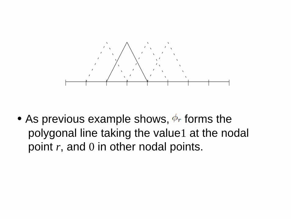
• As previous example shows, forms the polygonal line taking the value1 at the nodal point r, and 0 in other nodal points.

2004 Advanced Nonlinear Finite Element Method: Exercises1

• Verify [V ] from [B].(check the equations in the notes)• Eq.(24) sets v = u + w, explain the reason why we can have such

definition.• Using Eq.(47), express the Eq.(47) (check the equations in the notes)• With the region 0 < x < 1, and the number of partition n = 4, obtain the

element matrix as well as the compound matrix. In obtaining theelement matrix, remember to write out every matrix. Do not only write the last matrix obtained.

• Using Eq.(77), express the Eq.(97) (check the equation in the notes)• On the nodal point r, φr takes the value 1, but for the other nodal

points, φr takes the value 0, thus forms the polygonal line. Using φr, examine the polygonal line can be expressed in the form , as well as in the form , 1(r = s, r = s).