数値相対論の展開���Progress & Status of Numerical Relativity

Masaru ShibataYukawa Institute for Theoretical Physics

Kyoto University

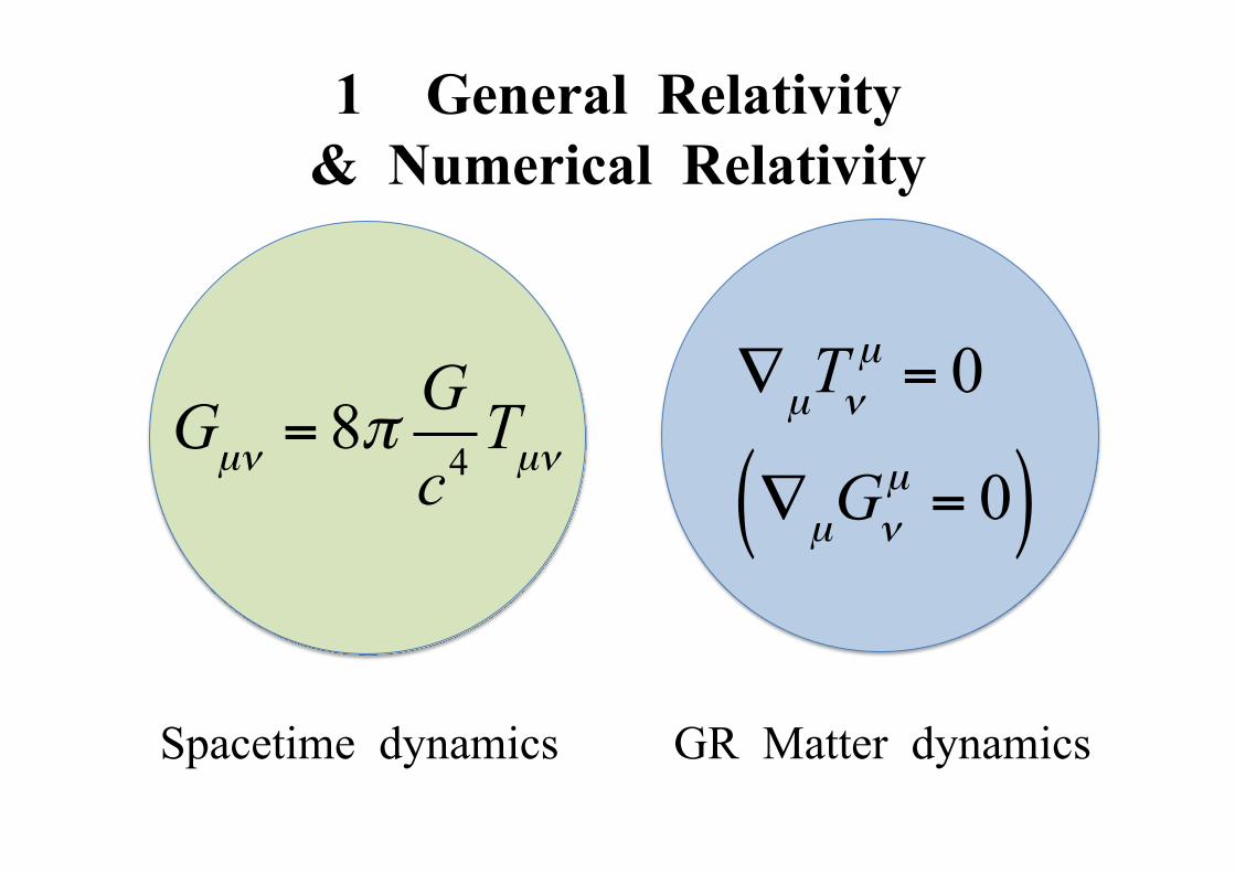
1 General Relativity & Numerical Relativity

Gµν = 8πGc4Tµν

∇µTνµ = 0

∇µGνµ = 0( )

Spacetime dynamics GR Matter dynamics

3

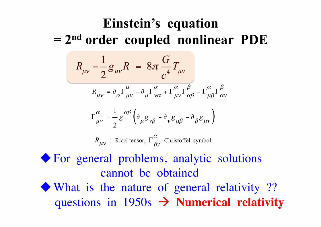
Einstein’s equation = 2nd order coupled nonlinear PDE

Rµν −12gµνR = 8π G

c4Tµν

Rµν

= ∂αΓµνα

− ∂µΓναα

+ ΓµναΓαββ

− ΓµβαΓανβ

Γµνα

=1

2gαβ

∂µgνβ

+ ∂νgµβ

− ∂βgµν( )

Rµν : Ricci tensor, Γβγα

: Christoffel symbol

u For general problems, analytic solutions cannot be obtainedu What is the nature of general relativity ?? questions in 1950s à Numerical relativity

4

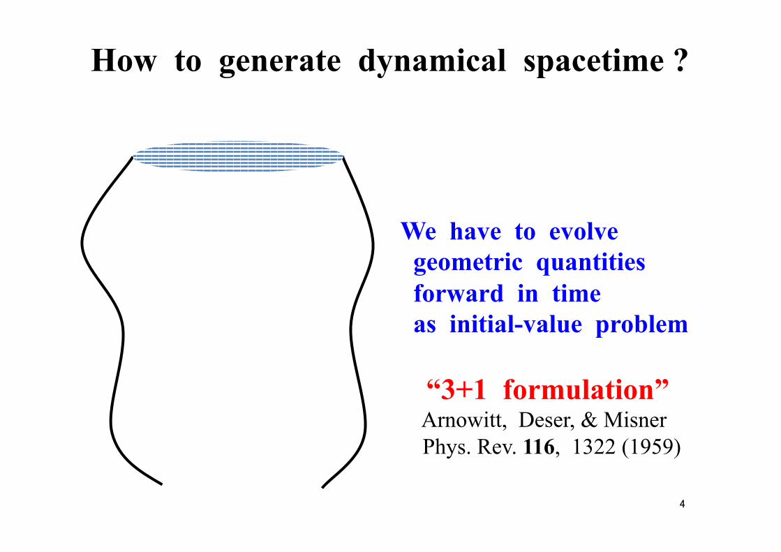
How to generate dynamical spacetime ?

We have to evolve geometric quantities forward in time as initial-value problem “3+1 formulation” Arnowitt, Deser, & Misner Phys. Rev. 116, 1322 (1959)

Time Unknown manifold

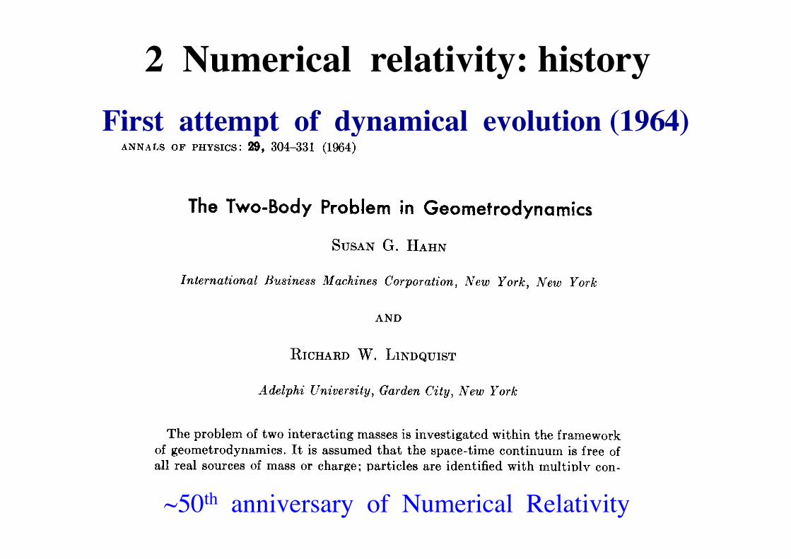
First attempt of dynamical evolution (1964) ANNALS OF PHYSICS: f8, 304-331 (1964)

The Two-Body Problem in Geometrodynamics

SUSAN G. HAHN

International Business Machines Corporation, New York, New York

AND

RICHARD W. LINDQUIST

Adelphi University, Garden City, New York

The problem of two interacting masses is investigated within the framework of geometrodynamics. It is assumed that the space-time continuum is free of all real sources of mass or charge; particles are identified with multiply con- nected regions of empty space. Particular attention is focused on an asymp- totically flat space containing a “handle” or “wormhole.” When the two “mouths” of the wormhole are well separated, they seem to appear as two cen- ters of gravitational attraction of equal mass. To simplify the problem, it is assumed that the metric is invariant under rotations about the axis of sym- metry, and symmetric with respect to the time t = 0 of maximum separation of the two mouths. Analytic initial value data for this case have been ob- tained by Misner; these contain two arbitrary parameters, which are uniquely determined when the mass of the two mouths and their initial separation have been specified. We treat a particular case in which the ratio of mass to initial separation is approximately one-half. To determine a unique solution of the remaining (dynamic) field equations, the coordinate conditions go- = -& are imposed; then the set of second order equations is transformed into a quasi- linear first order system and the difference scheme of Friedrichs used to ob- tain a numerical solution. Its behavior agrees qualitatively with that of the one-body problem, and can be interpreted as a mutual attraction and pinching- off of the two mouths of the wormhole.

I. INTRODUCTION

Wheeler (1, 2) has used the term “geometrodynamics” to characterize those solutions of the field equations for gravitation and electromagnetism’

41 = R,v - ?4 g& = 2(F,,FP - Pi gj,.F,sF=B) (l.la)

FPu;v = 0 (l.lb)

1 Throughout this paper Greek subscripts and superscripts range from 0 to 3 and Latin ones from 1 to 3. Also, units are chosen so that G (universal gravitation constant) = c = 1.

304

~50th anniversary of Numerical Relativity

2 Numerical relativity: history

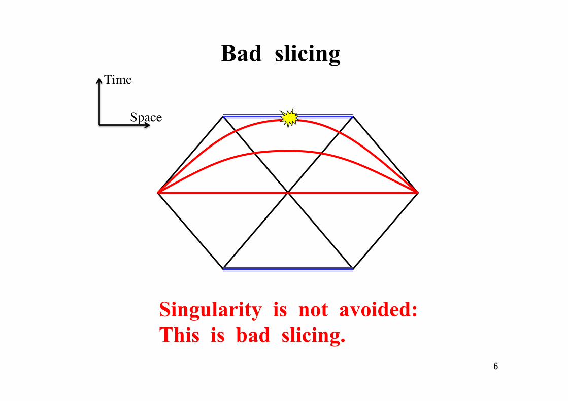
Bad slicing

Singularity is not avoided: This is bad slicing.

6

Time

Space

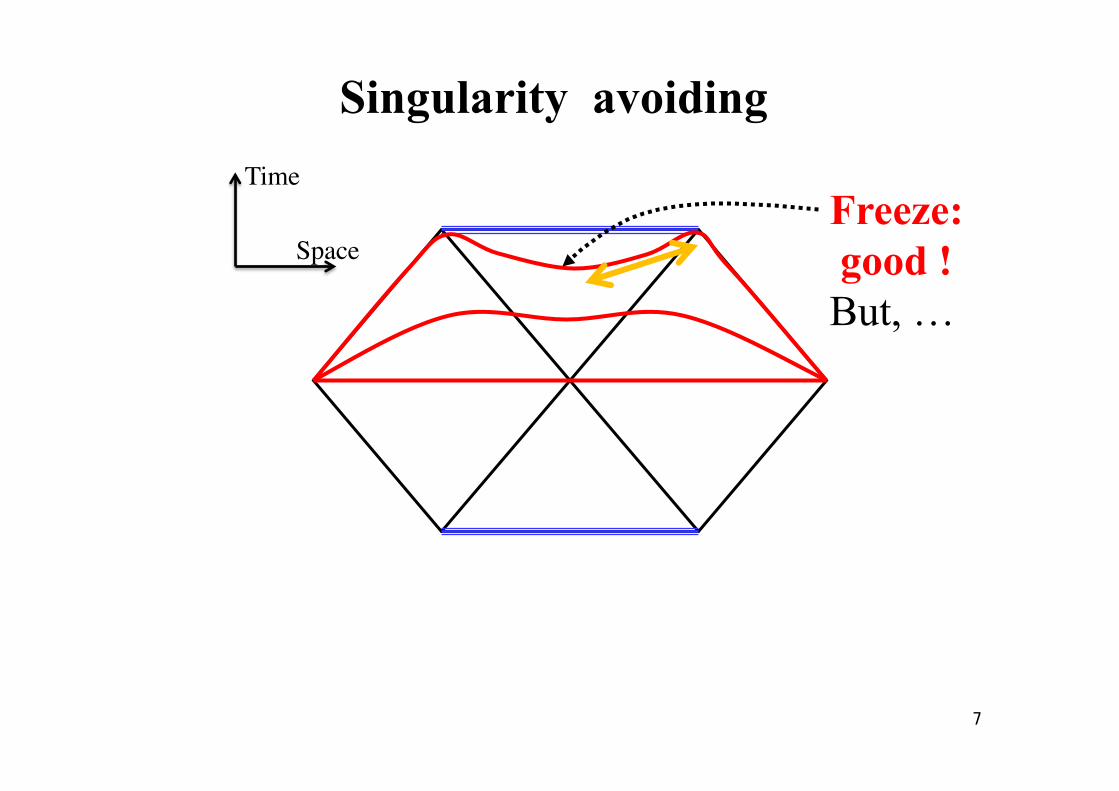
Singularity avoiding

7

Freeze: good ! But, …

Time

Space

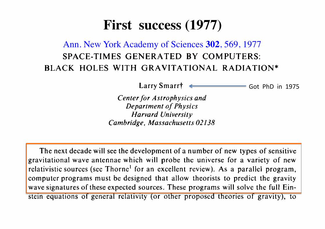
First success (1977)

SPACE-TIMES GENERATED BY COMPUTERS: BLACK HOLES WITH GRAVITATIONAL RADIATION*

Larry Smarr t Center for Astrophysics and

Department of Physics Harvard University

Cambridge, Massachusetts 02138

The next decade will see the development of a number of new types of sensitive gravitational wave antennae which will probe the universe for a variety of new relativistic sources (see Thorne’ for an excellent review). As a parallel program, computer programs must be designed that allow theorists to predict the gravity wave signatures of these expected sources. These programs will solve the full Ein- stein equations of general relativity (or other proposed theories of gravity), to build space-times containing colliding black holes or collapsing nonspherical stars.

Over the years a number of approaches have been devised to investigate por- tions of these spacetimes. The beautiful analytic work of Hawking,’ Carter,’ Robinson3 and others has led to the result that the final stationary state of collapse or collision to form a black hole is a Kerr-Newman black hole. The early stages of the complicated nonspherical magnetohydrodynamical collapse with fully rela- tivistic equations (assuming only a slowly time-varying gravitational field) has been computer coded by W i l ~ o n . ~ The late stages of gyrations around a black hole or neutron star have been worked out extensively using linear perturbation equa- tions off the fully relativistic background.’

The only piece left is the fully relativistic, highly dynamic, nonperturbative, strong field interaction region in which most of the processes of interest to gravity wave astronomy lie ( ix . , here is where the gravitational field comes into its own right as the primary dynamical entity.) One would like to be able to use computers to follow this region in detail the way other classical field theories do, e.g., hydro- dynamics, electrodynamics, aerodynamics, etc. Kenneth Eppley and I have written such a program for the axisymmetric vacuum Einstein equations. We, as well as others, are currently extending this to cases of matter coupling and fully four dimensional space-times (i.e., no spatial symmetry). This article will attempt to give an overview of what goes into and what comes out of such an endeavor.

SPACE-TIME KINEMATICS

When no strong gravitational fields are present, physics can be described by special relativity. Here the space-time metric has no dynamical freedom but is given by the globally Poincari-invariant Minkowski space-time. Because of the time and space translational invariance, there exist preferred time and space coordinates. I f one defines a set of Eulerian observers as those timelike worldlines

*This work was supported in part by the National Science Foundation. ?Junior Fellow, Harvard Society of Fellows.

569

Ann. New York Academy of Sciences 302, 569, 1977

Got    PhD    in    1975

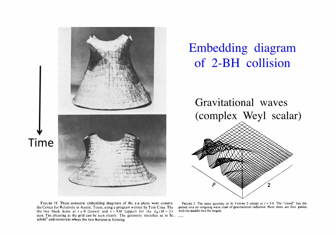
Embedding diagram of 2-BH collision

Srnarr: Cornputer-Generated Space-Times

using ZFL for hyperbolic head on c ~ l l i s i o n s : ~ ~

597

Evaluation of this formula (see FIGURE 20) shows that t drops below 1% by the time v , <, 0.5. For lower values of v, , the ZFL underestimates the actual effi-

F I G U R E 19. These isometric embedding diagrams of the z-p plane were constructed at the Center for Relativity in Austin, Texas, using a program written by Tom Criss. They show the two black holes at i = 0 (lower) and t = 9 M (upper) [or the L o / M = 3.9 colli- sion. The shearing at the grid can be seen clearly. The geometry stretches as in Schwarz- schild’ and constricts where the new horizon is forming.

FIGURE 3 . The same quantity as in FIGURE 2 except at f = 5.4. The “cloud” has dis- persed into an outgoing wave train of gravitational radiation. Note there are four pulses, with the middle two the largest.

FIGURE 4. A contour plot or r2f as shown in FIGURE 3. This clearly shows the quadrupolar nature of the radiation, which should have angular dependence -sin4@, where 0 = 0 on the z-axis.

582

Time

Gravitational waves (complex Weyl scalar)

1876

Progress of Theoretical Physics, Vol. 65, No.6, June 1981

General Relativistic Collapse of Axially Symmetric Stars Leading

to the Formation of Rotating Black Holes

Takashi NAKAMURA

Research Institute for Fundamental Physics Kyoto University, Kyoto 606

(Received November 1, 1980)

Numerical calculations have been made for the formation process of axisymmetric, rotating black holes of 10M0. The initial density of a star is about 3x 1013 g/ cm'. Numerical results are classified mainly by q which corresponds to lal/M in a Kerr black hole. For q:S0.3, the effect of rotation to the gravitational collapse is only to make the shape of matter oblate. For 0.3:SqS:;0.95, although the distribution of matter is disk·like, a ring-like peak of proper density appears. This ring is inside the apparent horizon, which is always formed in the case q:S 0.95. For q<:0.95, no apparent horizon is formed. The distribution of matter shows a central disk plus an expanding ring. It is found that electromagnetic-like field in the [(2+1)+1]-formalism plays an important role in a formation of a rotating black hole. Local conservation of angular momentum is checked. Accuracy of constraint equations is also shown to see the truncation error in the numerical calculations.

§ 1. Introduction

Stationary solutions to Einstein's vacuum field equations have been studied very well. On the assumption that all singularities in space-time are hidden behind the non-singular event horizon, the Israel-Carterl),Z) theorem tells us that solutions form discrete continuous families each depending on, at most, two parameters. Robinson3

) proved that the Kerr family with lal < M is the unique one of the Israel-Carter theorem. On the other hand if the above assumption is not adopted many other stationary solutions4

) have been obtained. In the realistic gravitational collapse a star collapses from the region of slow

motion and weak gravity to that of fast motion and strong gravity. The struc-ture of the latter region will depend on the initial conditions. Therefore neither the assumption on this structure nor the special stationary solution but the dynamical process does determine the ultimate fate of the gravitational collapse. For a spherically symmetric case, Yodzis et al. 5) showed a possibility of the existence of a naked singularity. For a non-spherical case, Nakamura et al. 6

)

suggested that a naked singularity may appear in a prolate collapse if the initial quadrupole moment is large enough. These results tell us that naked singularity may appear in the realistic collapse of a star under a certain initial condition.

To know the dynamical process of collapse of a star, it is necessary to inte-

at Library of Research R

eactor Institute, Kyoto U

niversity on September 6, 2015

http://ptp.oxfordjournals.org/D

ownloaded from

First multi-D non-vacuum &

dynamical solution

Born    in      09/18/1950

General Relativistic Collapse 0/ Axially Symmetric Stars 1885

A.C.Eq. should be zero if we can solve the basic equations exactly. In numerical calculation, A.C.Eq. tells us the effect of the truncation error and the viscosity terms to the true solution quantitatively. A.C.Eq.'s for M64 are shown in Fig. 2. For simplicity the time variation of A.C.Eq.'s at the center is shown. We can see the accuracy of momentum constraint equations (Eq. (2·6)) is worse than that of the Hamiltonian (Eq. (2·5)) and the angular momentum constraint equations (Eq. (2·9)). As XAB is determined by the second and the first derivative of the metric tensor, the accuracy of the momentum constraint equations is essentially that of the third derivative of the metric tensors. On the other hand the accuracy of the Hamiltonian constraint equation is essentially that of the second derivative of the metric tensors and the accuracy of the angular momentum constraint equation is essentially that of the first derivative of EA. Figure 2 shows A. C. Eq.'s are 20% or so at the time when an apparent horizon is formed. Therefore it can be said that the accuracy of our numerical calculation is good enough.

The numerical results are summarized as follows. For slowly rotating models, for example M32, the distribution of p and Qb becomes oblate shape as the collapse proceeds. An apparent horizon is formed and matter is swallowed into the black hole completely. In this case the effect of rotation is only to deform the matter distribution. For rather rapidly rotating models, for example M80, the shape of Qb is disk-like (Fig. 3 (a)) but there appears a ring-like peak of p which is inside the apparent horizon (Fig. 3 (b)). At this peak EAEA is very large (Fig. 3 (b)) and m takes a minimum value (Table I). The reason for this behavior can be interpreted as the general relativistic effect of rotation. Taking a trace of Eq. (2'2), we have

TlME=1.20E.01 0.452E-01

j 5 6 R

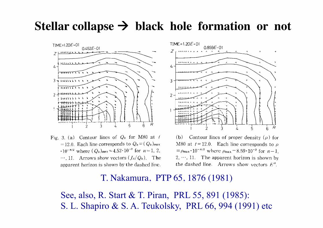
Fig. 3. (a) Contour Jines of Qb for M80 at = 12.0. Each line corresponds to Qb = (Qb )max '1O- n /2 where (Qb)max=4.52·10- 2 for n=l, 2, "',11. Arrows show vectors (fA/Qb). The apparent horizon is shown by the dashed line.

TIME= 1.20E .01 0.859E-01

Z ••• " •••••

4

3

2

(b) Contour lines of proper density (p) for M80 at 1=12.0. Each line corresponds to p

=Pmax'10- n/2 where Pmax=8.59·10- 2 for n=l,

2, "', 11. The apparent horizon is shown by the dashed line. Arrows show vectors EA

at Library of Research R

eactor Institute, Kyoto U

niversity on September 6, 2015

http://ptp.oxfordjournals.org/D

ownloaded from

T. Nakamura, PTP 65, 1876 (1981)

Stellar collapse à black hole formation or not

See, also, R. Start & T. Piran, PRL 55, 891 (1985): S. L. Shapiro & S. A. Teukolsky, PRL 66, 994 (1991) etc

Progress in the last quarter of century���(1990s ~)

Two major motivations: •  Gravitational-wave detection has become a

realistic (not joking) project since early 1990: GWs exist (Hulse-Taylor pulsar) and have to be detected

•  High-energy phenomena have been discovered: e.g., gamma-ray bursts ~ dynamical BH + torus

Accurate & physical simulations are required for solid obs. projects: excellent driving force !

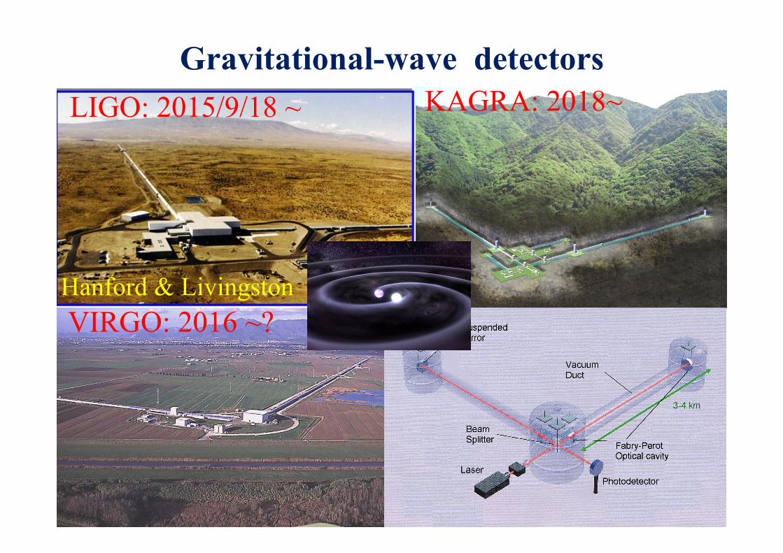
Gravitational-wave detectors LIGO: 2015/9/18 ~

VIRGO: 2016 ~?

KAGRA: 2018~

Hanford & Livingston

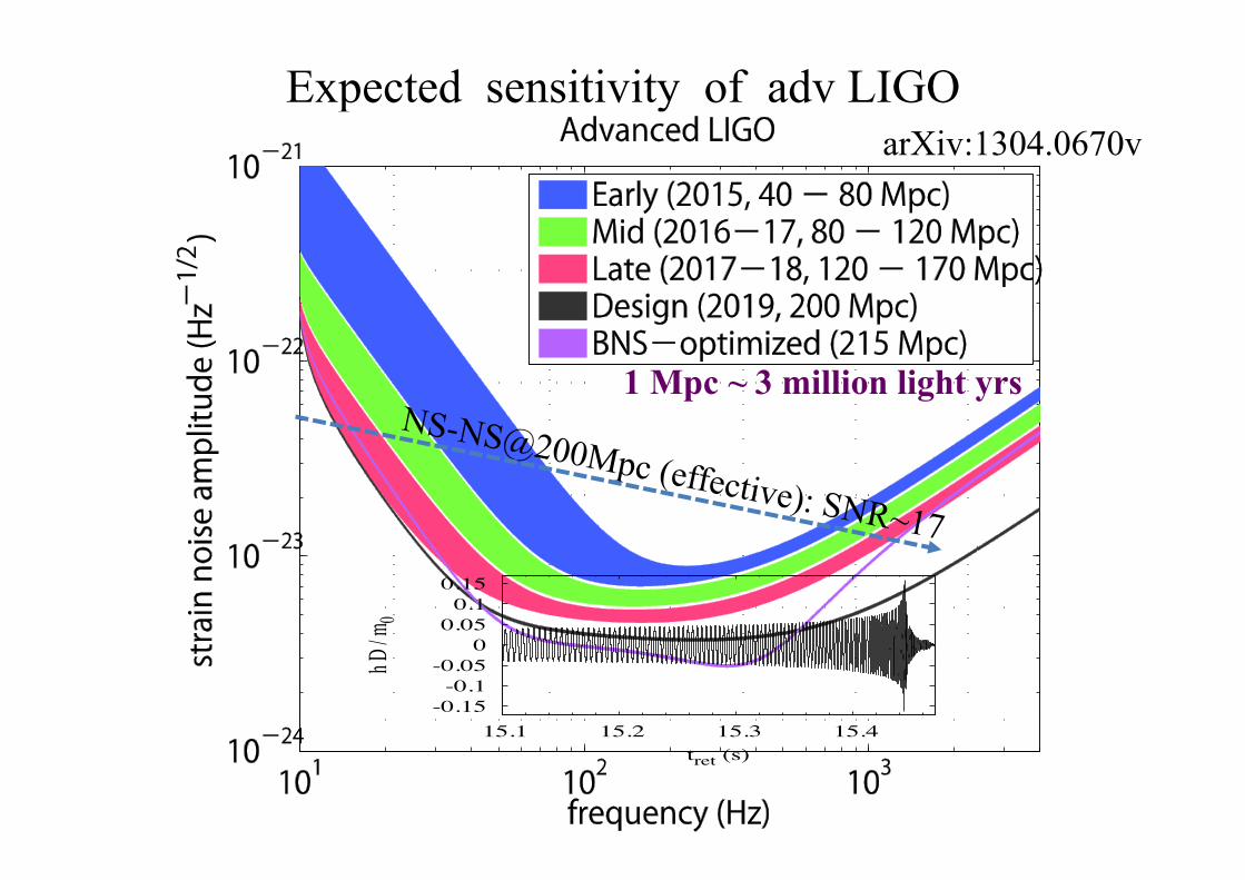
Expected sensitivity of adv LIGO

NS-NS@200Mpc (effective): SNR~17

arXiv:1304.0670v

1 Mpc ~ 3 million light yrs

-0.15-0.1

-0.05 0

0.05 0.1

0.15

15.1 15.2 15.3 15.4

h D / m

0

tret (s)

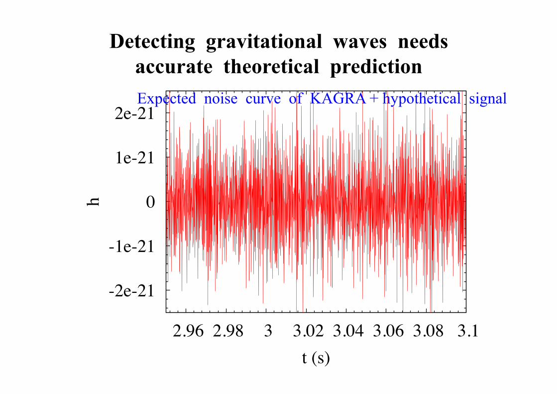
Detecting gravitational waves needs accurate theoretical prediction

-2e-21

-1e-21

0

1e-21

2e-21

2.96 2.98 3 3.02 3.04 3.06 3.08 3.1

h

t (s)

Expected noise curve of KAGRA + hypothetical signal

Detecting gravitational waves needs accurate theoretical prediction

-2e-21

-1e-21

0

1e-21

2e-21

2.96 2.98 3 3.02 3.04 3.06 3.08 3.1

h

t (s)

SNR~10 event

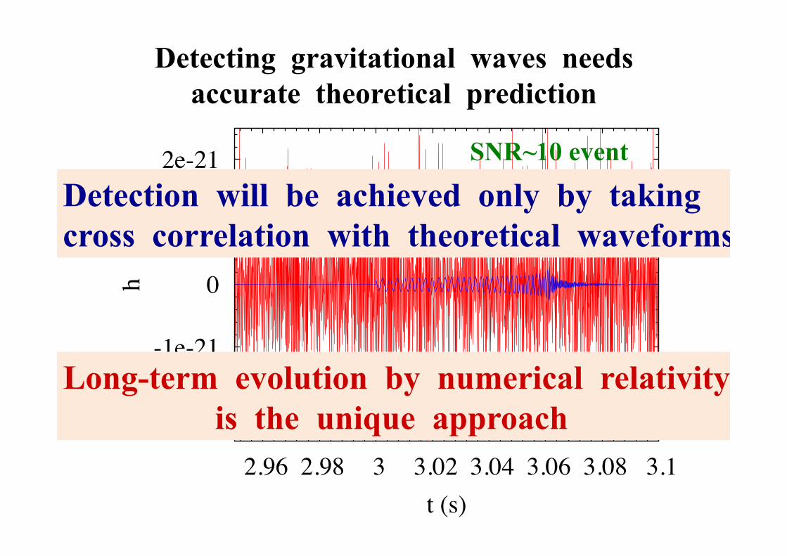
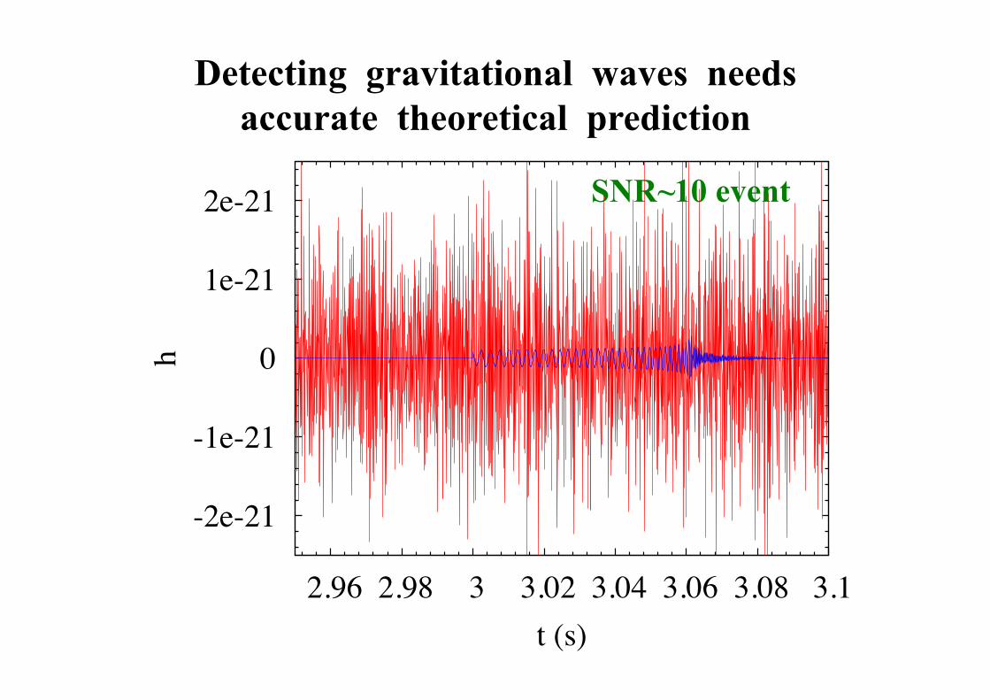
Detecting gravitational waves needs accurate theoretical prediction

-2e-21

-1e-21

0

1e-21

2e-21

2.96 2.98 3 3.02 3.04 3.06 3.08 3.1

h

t (s)

SNR~10 event

Detection will be achieved only by taking cross correlation with theoretical waveforms

Long-term evolution by numerical relativity is the unique approach

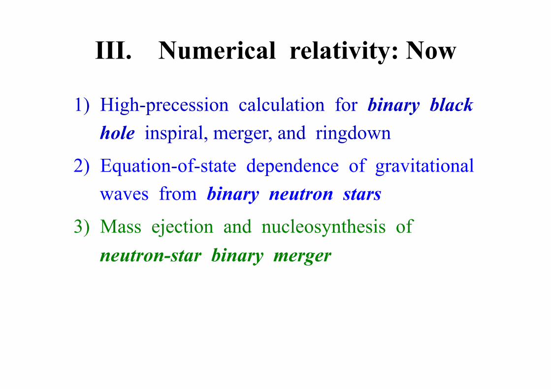
III. Numerical relativity: Now

1)  High-precession calculation for binary black hole inspiral, merger, and ringdown

2)  Equation-of-state dependence of gravitational waves from binary neutron stars

3)  Mass ejection and nucleosynthesis of neutron-star binary merger

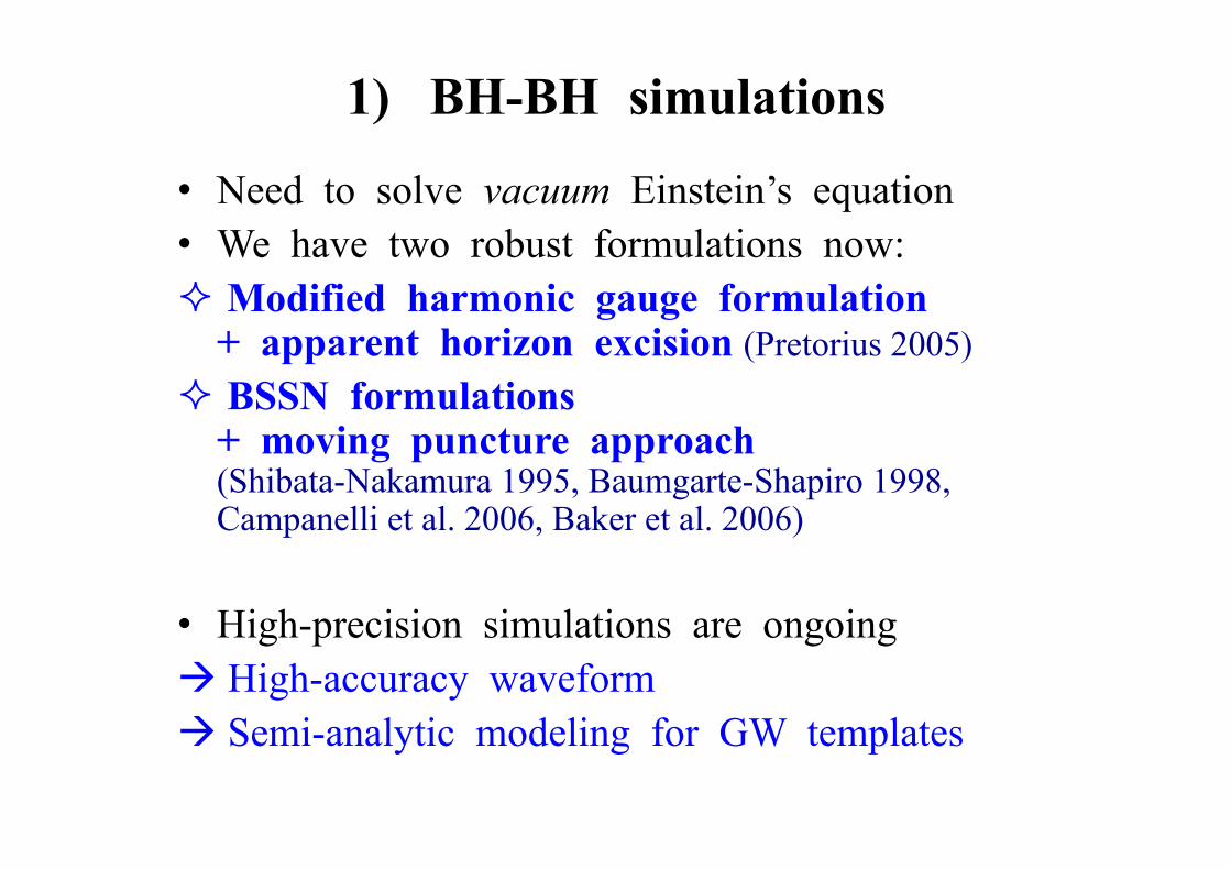
1) BH-BH simulations

•  Need to solve vacuum Einstein’s equation •  We have two robust formulations now: ²  Modified harmonic gauge formulation

+ apparent horizon excision (Pretorius 2005) ²  BSSN formulations

+ moving puncture approach (Shibata-Nakamura 1995, Baumgarte-Shapiro 1998, Campanelli et al. 2006, Baker et al. 2006)

•  High-precision simulations are ongoing à  High-accuracy waveform à  Semi-analytic modeling for GW templates

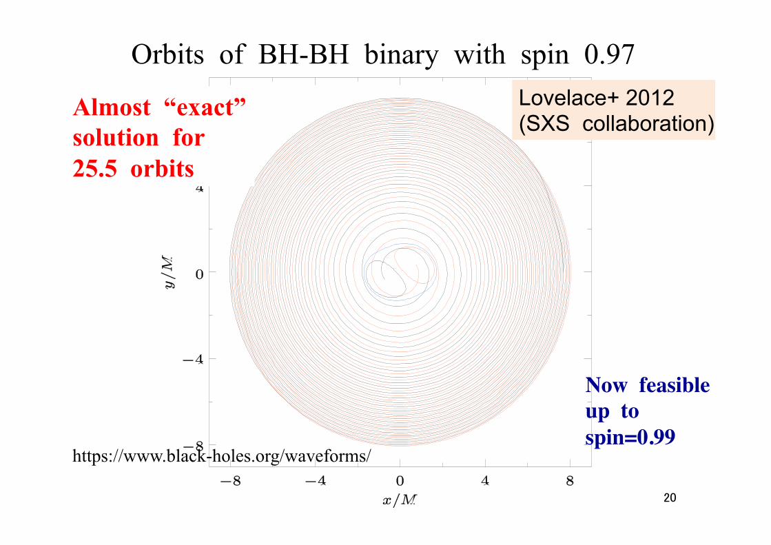
Orbits of BH-BH binary with spin 0.97

20

Lovelace+ 2012 (SXS collaboration)

Almost “exact” solution for 25.5 orbits

Now feasible up tospin=0.99

https://www.black-holes.org/waveforms/

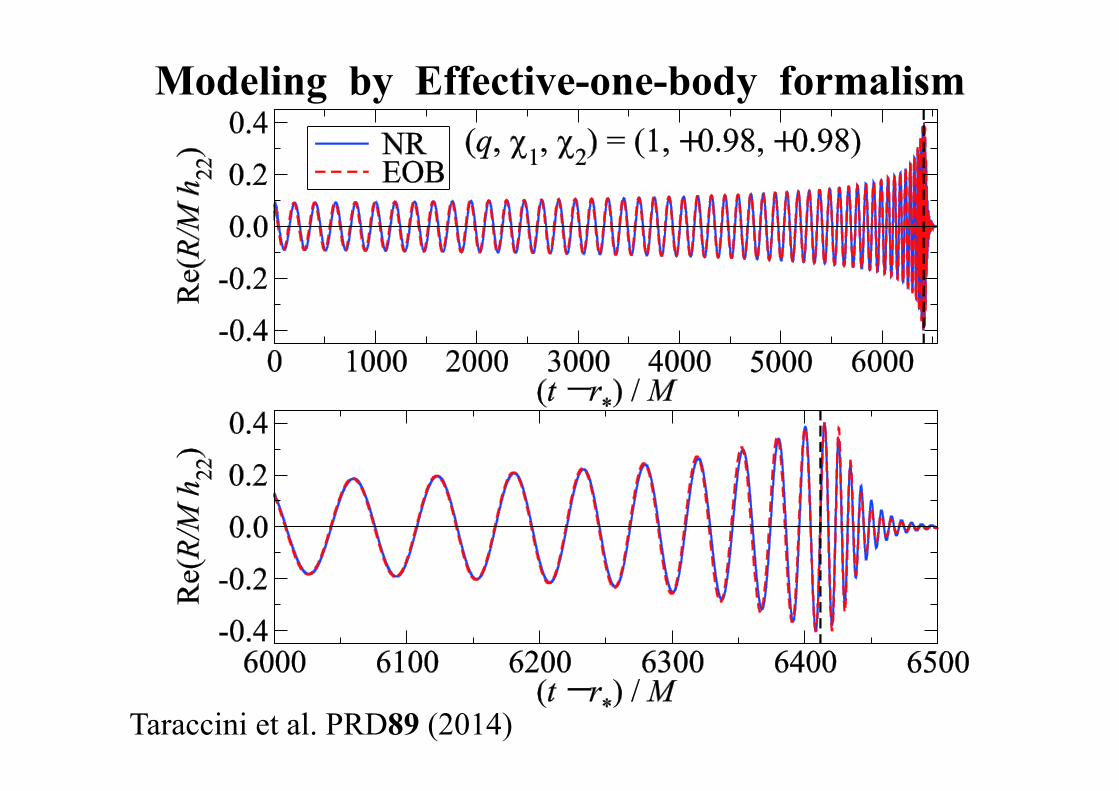
Modeling by Effective-one-body formalism

Taraccini et al. PRD89 (2014)

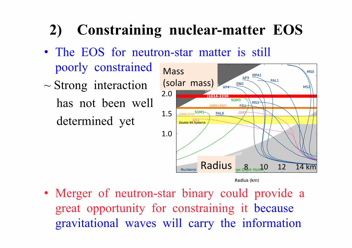
2) Constraining nuclear-matter EOS

•  The EOS for neutron-star matter is still poorly constrained

~ Strong interaction has not been well determined yet

•  Merger of neutron-star binary could provide a

great opportunity for constraining it because gravitational waves will carry the information

2.0    1.5    1.0

   8            10          12          14  km Radius

Mass  (solar    mass)

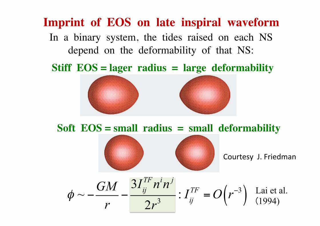
Imprint of EOS on late inspiral waveform In a binary system, the tides raised on each NS depend on the deformability of that NS:

Courtesy    J.  Friedman

Stiff EOS = lager radius = large deformability

Soft EOS = small radius = small deformability

φ ~ −GMr

−3Iij

TFnin j

2r3: Iij

TF =O r−3( ) Lai et al. (1994)

-0.15-0.1

-0.05 0

0.05 0.1

0.15

0 10 20 30 40 50 60 70

h D

/ m

0

tret (ms)

APR4ALF2

H4

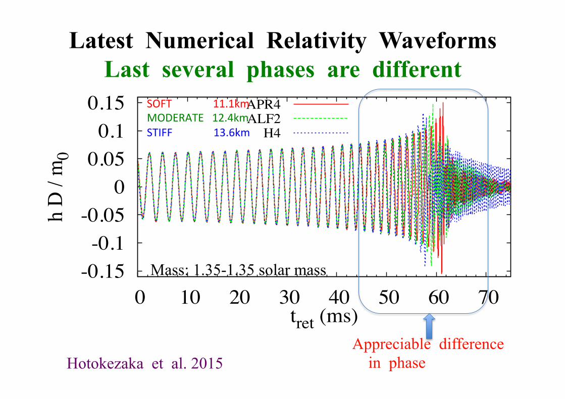
Latest Numerical Relativity Waveforms Last several phases are different

Hotokezaka et al. 2015

Mass: 1.35-1.35 solar mass

SOFT                              11.1km  MODERATE      12.4km  STIFF                              13.6km

Appreciable difference in phase

10-23

10-22

0.2 0.3 0.5 0.8 1 2 3 4

2|h(

f)| (D

eff=

100

Mpc

)

f (kHz)

APR4SFHoDD2

TMA TM1 BBH

aLIGO

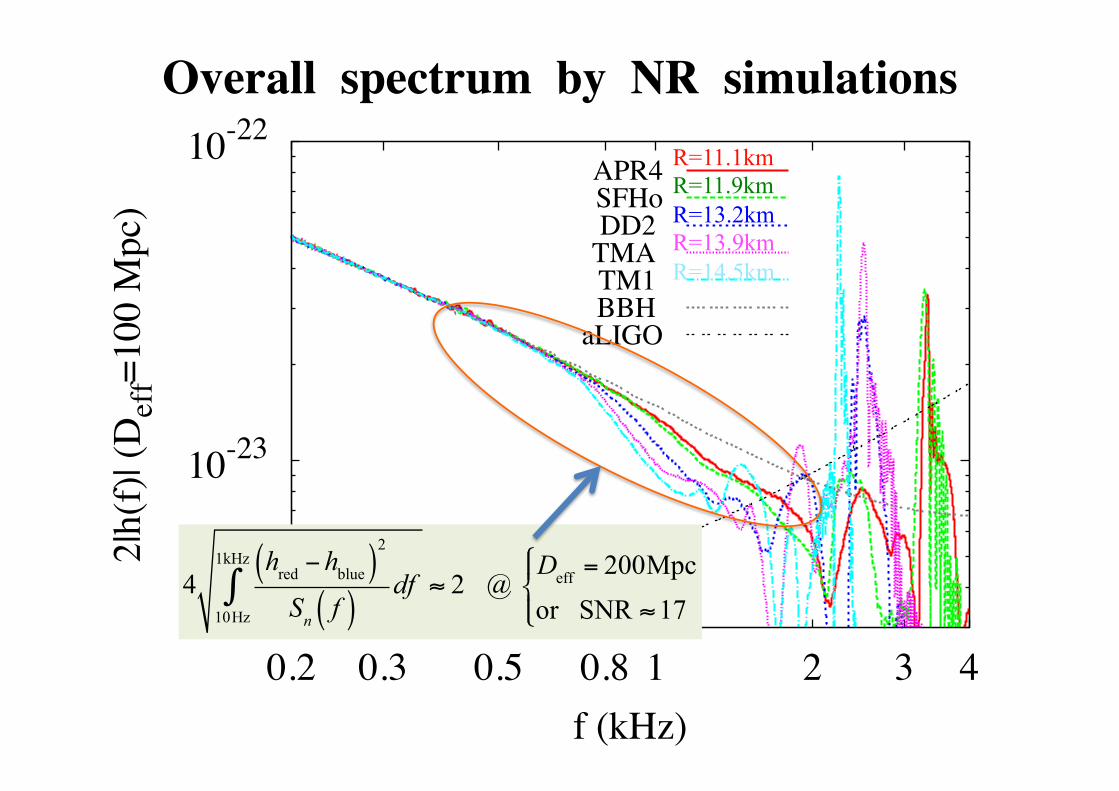
Overall spectrum by NR simulations

4hred − hblue( )

2

Sn f( )df

10Hz

1kHz

∫ ≈ 2 @ Deff = 200Mpc

or SNR ≈17

$%&

'&

R=11.1km R=11.9km R=13.2km R=13.9km R=14.5km

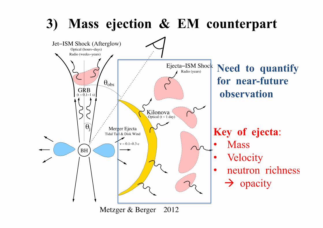
3) Mass ejection & EM counterpart

BH

θobs

θjTidal Tail & Disk Wind

Ejecta−ISM Shock

Merger Ejecta

v ~ 0.1−0.3 c

Optical (hours−days)

KilonovaOptical (t ~ 1 day)

Jet−ISM Shock (Afterglow)

GRB(t ~ 0.1−1 s)

Radio (weeks−years)

Radio (years)

Metzger & Berger 2012

Key of ejecta: •  Mass •  Velocity •  neutron richness à opacity

Need to quantify for near-future observation

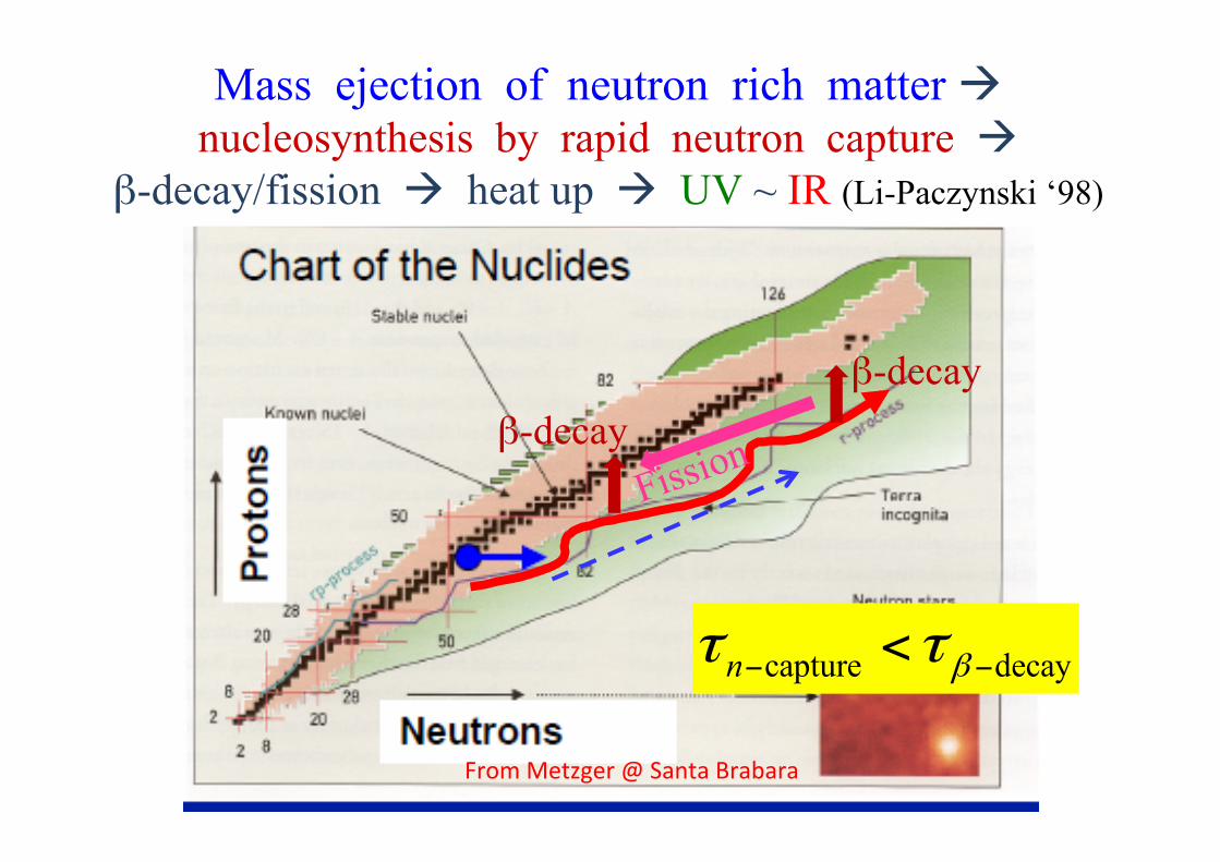
β-decay

From  Metzger  @  Santa  Brabara

Mass ejection of neutron rich matter à nucleosynthesis by rapid neutron capture à　

β-decay/fission à heat up à UV ~ IR (Li-Paczynski ‘98)

capture decayn βτ τ− −<

β-decay

28

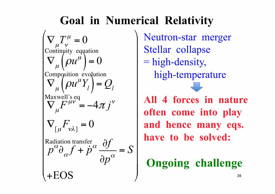
Goal in Numerical Relativity ∇µTν

µ = 0

∇µ ρuµ( ) = 0∇µ ρuµYl( ) =Ql∇µF

µν = −4π jν

∇[µFνλ ] = 0

pα∂α f + !pα ∂f∂pα

= S

+EOS

$

%

&&&&&&&&&&&&&

'

(

)))))))))))))

Neutron-star merger Stellar collapse = high-density, high-temperature All 4 forces in nature often come into play and hence many eqs. have to be solved: Ongoing challenge

Composition evolution

Maxwell’s eq

Radiation transfer

Continuity equation

29

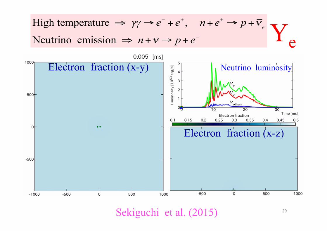
Electron fraction (x-y)

Electron fraction (x-z)

νeνeνothers

High temperature ⇒ γγ→ e− + e+ , n+ e+ → p+νeNeutrino emission ⇒ n+ν→ p+ e−

Sekiguchi et al. (2015)

Ye

Neutrino luminosity

Simulation results for different EOSs

This-time case

A broad distribution of Ye is likely

Sekiguchi et al. 2015

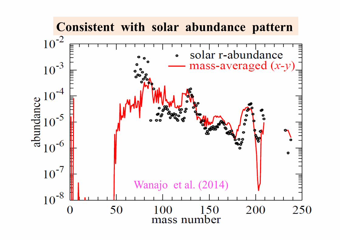
Consistent with solar abundance pattern

Wanajo et al. (2014)

Summary

•  After long-term (~50 years) efforts, numerical relativity has become a mature field

•  Many “observationally-motivated” simulations are ongoing à Templates of gravitational waves & prediction for EM counterparts

•  Numerical relativity will contribute to solving unsolved issues in GW physics, astronomy/astrophysics & nuclear physics in the next decade

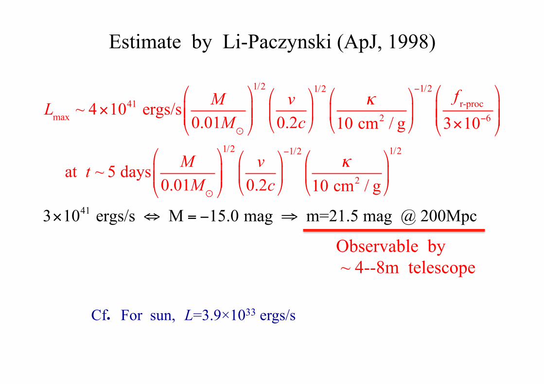
Estimate by Li-Paczynski (ApJ, 1998)

Lmax ~ 4×1041 ergs/s M0.01M⊙

"

#$$

%

&''

1/2v

0.2c"

#$

%

&'

1/2κ

10 cm2 / g

"

#$

%

&'

−1/2 f r-proc

3×10−6

"

#$$

%

&''

at t ~ 5 days M0.01M⊙

"

#$$

%

&''

1/2v

0.2c"

#$

%

&'

−1/2κ

10 cm2 / g

"

#$

%

&'

1/2

3×1041 ergs/s ⇔ M = −15.0 mag ⇒ m=21.5 mag @ 200Mpc

Observable by ~ 4--8m telescope

Cf.    For sun,  L=3.9×1033 ergs/s