t-tests. interval estimation and the t distribution
TRANSCRIPT

t-Tests

Interval Estimation and the t Distribution

PSYC 6130, PROF. J. ELDER 3
Large Sample z-Test
• Sometimes we have reason to test hypotheses involving specific values for the mean.– Example 1. Claim: On average, people sleep less than the often
recommended eight hours per night.
– Example 2. Claim: On average, people drink more than the recommended 2 drinks per day.
– Example 3. Claim: On average, women take more than 4 hours to run the marathon.
• However, it is rare that we have a specific hypothesis about the standard deviation of the population under study.
• For these situations, we can use the sample standard deviation s as an estimator for the population standard deviation .
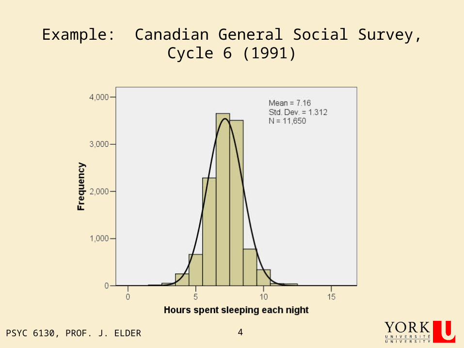
• If the sample size is pretty big (e.g., >100), then this estimate is pretty good, and we can just use the standard z test.
PSYC 6130, PROF. J. ELDER 4
Example: Canadian General Social Survey, Cycle 6 (1991)
PSYC 6130, PROF. J. ELDER 5
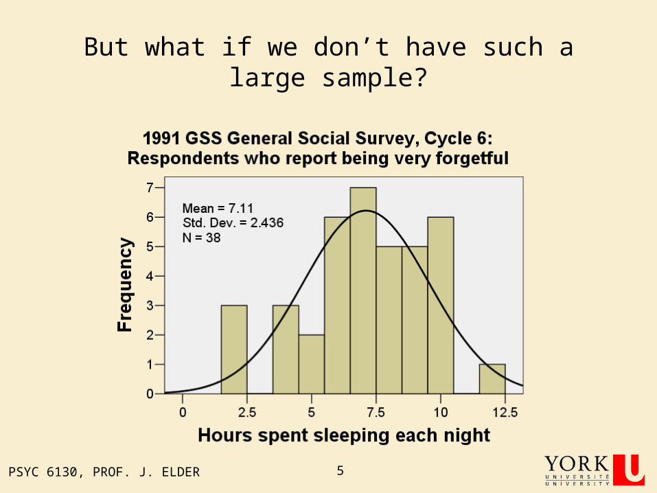
But what if we don’t have such a large sample?

PSYC 6130, PROF. J. ELDER 6
Student’s t Distribution
• Problem: for small n, s is not a very accurate estimator of .
• The result is that the computed z-score will not follow a standard normal distribution.
• Instead, the standardized score will follow what has become known as the Student’s t distribution.
-
X
Xt
swhere
X
ss
n
PSYC 6130, PROF. J. ELDER 7
Student’s t Distribution
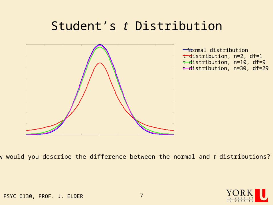
Normal distributiont distribution, n=2, df=1t distribution, n=10, df=9t distribution, n=30, df=29
How would you describe the difference between the normal and t distributions?
PSYC 6130, PROF. J. ELDER 8
Student’s t distribution
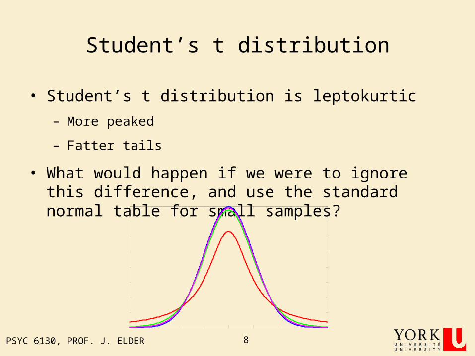
• Student’s t distribution is leptokurtic
– More peaked
– Fatter tails
• What would happen if we were to ignore this difference, and use the standard normal table for small samples?

PSYC 6130, PROF. J. ELDER 9
Student’s t Distribution
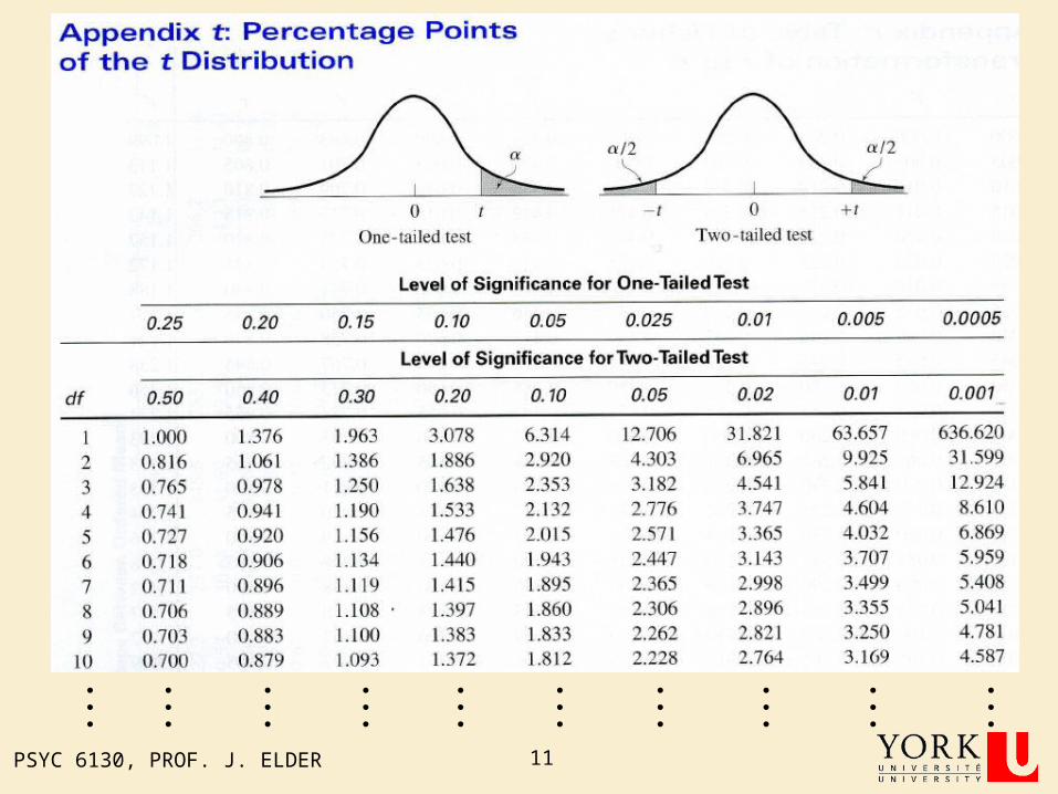
• Critical t values decrease as df increases
• As df infinity, critical t values critical z values
• Using the standard normal table for small samples would result in an inflated rate of Type I errors.
PSYC 6130, PROF. J. ELDER 10
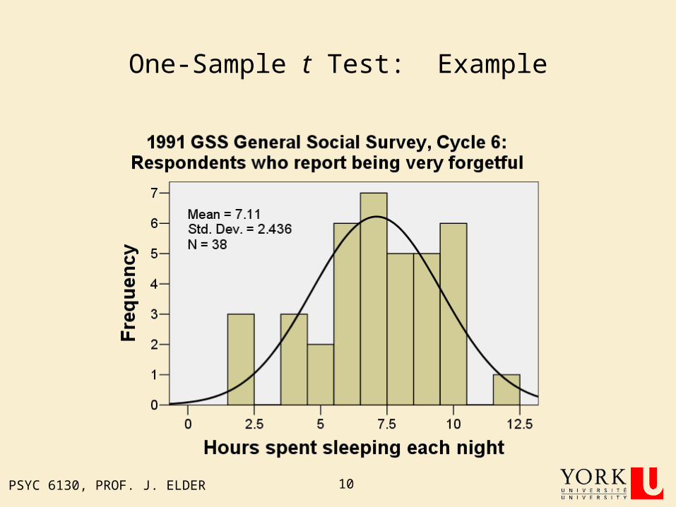
One-Sample t Test: Example
PSYC 6130, PROF. J. ELDER 11

PSYC 6130, PROF. J. ELDER 12
Reporting Results
• Respondents who report being very forgetful sleep, on average, 7.11 hours/night, significantly less than the recommended 8 hours/night, t(37)=2.25, p<.05, two-tailed.

PSYC 6130, PROF. J. ELDER 13
Confidence Intervals
• NHT allows us to test specific hypotheses about the mean.
– e.g., is < 8 hours?
• Sometimes it is just as valuable, or more valuable, to know the range of plausible values.
• This range of plausible values is called a confidence interval.
PSYC 6130, PROF. J. ELDER 14
Confidence Intervals
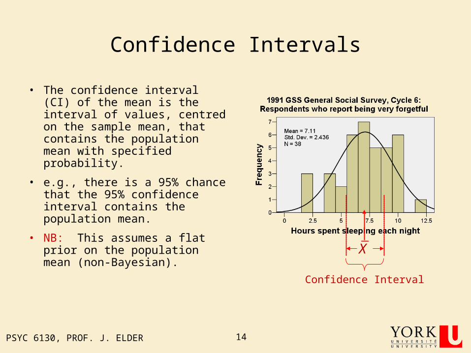
• The confidence interval (CI) of the mean is the interval of values, centred on the sample mean, that contains the population mean with specified probability.
• e.g., there is a 95% chance that the 95% confidence interval contains the population mean.
• NB: This assumes a flat prior on the population mean (non-Bayesian).
X
Confidence Interval

PSYC 6130, PROF. J. ELDER 15
Confidence Intervals
( )p
X
Xs
.025p .025p95% Confidence Interval

PSYC 6130, PROF. J. ELDER 16
Basic Procedure for Confidence Interval Estimation
1. Select the sample size (e.g., n = 38)
2. Select the level of confidence (e.g., 95%)
3. Select the sample and collect the data (Random sampling!)
4. Calculate the limits of the interval
XX
Xt X s t
s
/ 2XX s t
/ 2XX s t
End of Lecture 4
Oct 8, 2008
PSYC 6130, PROF. J. ELDER 18
Selecting Sample Size
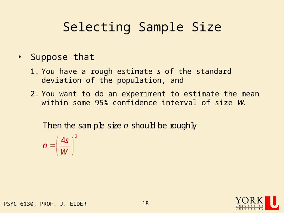
• Suppose that
1. You have a rough estimate s of the standard deviation of the population, and
2. You want to do an experiment to estimate the mean within some 95% confidence interval of size W.
2
Then the sample size should be r y
4
oughl
sn
W
n

PSYC 6130, PROF. J. ELDER 19
Assumptions Underlying Use of the t Distribution for NHT and Interval Estimation
• Same as for z test:
– Random sampling
– Variable is normal
• CLT: Deviations from normality ok as long as sample is large.
– Dispersion of sampled population is the same as for the comparison population

Sampling Distribution of the Variance
PSYC 6130, PROF. J. ELDER 21
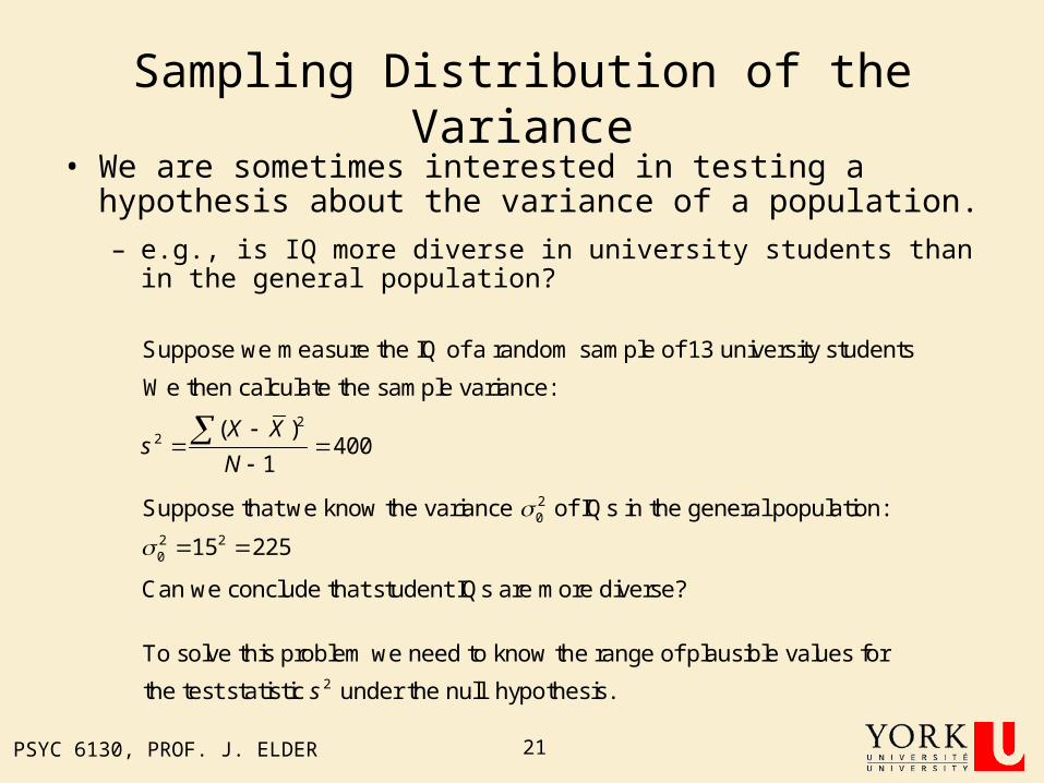
Sampling Distribution of the Variance• We are sometimes interested in testing a hypothesis
about the variance of a population.
– e.g., is IQ more diverse in university students than in the general population?
Suppose we measure the IQ of a random sample of 13 university students
We then calculate the sample variance:2
2 ( )400
1
X Xs
N
20
2 20
Suppose that we know the variance of IQs in the general population:
15 225
Can we conclude that student IQs are more diverse?
2
To solve this problem we need to know the range of plausible values for
the test statistic under the null hypothesis.s
PSYC 6130, PROF. J. ELDER 22
Sampling Distribution of the Variance
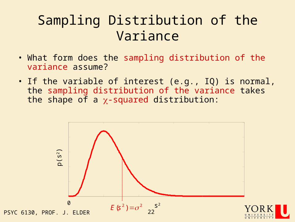
• What form does the sampling distribution of the variance assume?
• If the variable of interest (e.g., IQ) is normal, the sampling distribution of the variance takes the shape of a -squared distribution:
0
p(s2 )
s22 2( )E s
PSYC 6130, PROF. J. ELDER 23
Sample Variances and the -Square Distribution
2
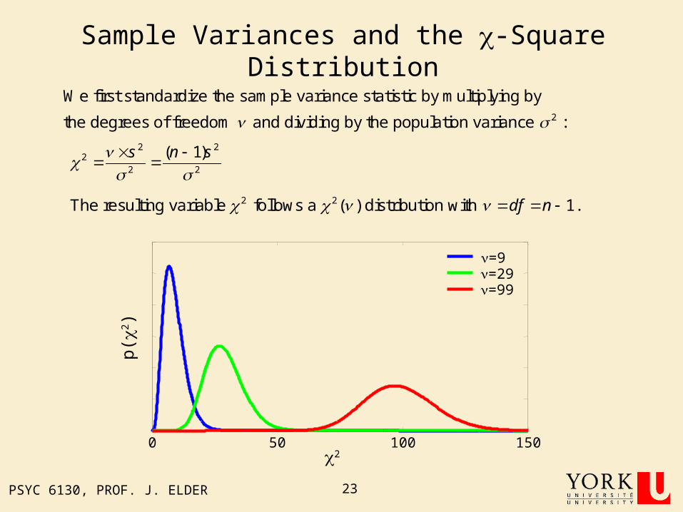
We first standardize the sample variance statistic by multiplying by
the degrees of freedom and dividing by the population variance :
2 2
22 2
( 1)s n s
2 2The resulting variable follows a ( ) distribution with 1.df n
0 50 100 150
=9=29=99
p(2 )
2
PSYC 6130, PROF. J. ELDER 24
Sample Variances and the -Square Distribution
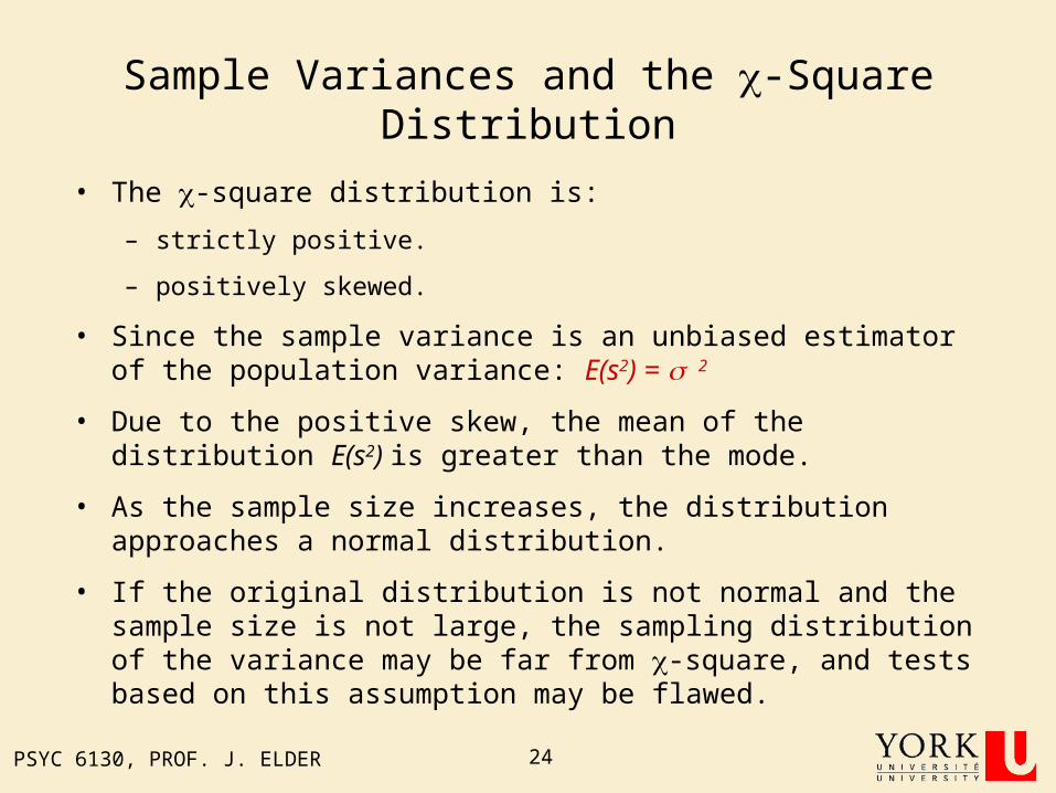
• The -square distribution is:
– strictly positive.
– positively skewed.
• Since the sample variance is an unbiased estimator of the population variance: E(s2) = 2
• Due to the positive skew, the mean of the distribution E(s2) is greater than the mode.
• As the sample size increases, the distribution approaches a normal distribution.
• If the original distribution is not normal and the sample size is not large, the sampling distribution of the variance may be far from -square, and tests based on this assumption may be flawed.
PSYC 6130, PROF. J. ELDER 25
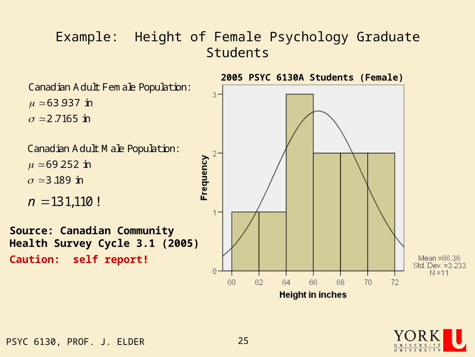
Example: Height of Female Psychology Graduate Students
Canadian Adult Female Population:
63.937 in
2.7165 in
Canadian Adult Male Population:
69.252 in
3.189 in
Source: Canadian Community Health Survey Cycle 3.1 (2005)
131,110!n
Caution: self report!
2005 PSYC 6130A Students (Female)
PSYC 6130, PROF. J. ELDER 26
Properties of Estimators
• We have now met two statistical estimators:
is an estimator for .X 2 2 is an estimator for .s
Both of these estimator
Unbiased
s are:
, i.e.,
( )= E X 2 2( )= E s
Consistent, i.e.,
the quality of the estimate improves as the sample size increases.
Efficient, i.e.,
given a fixed sample size, the accuracy of these estimators is better than
competing estimators.
NHT for Two Independent Sample Means

PSYC 6130, PROF. J. ELDER 28
Conditions of Applicability
• Comparing two samples (treated differently)
• Don’t know means of either population
• Don’t know variances of either population
• Samples are independent of each other
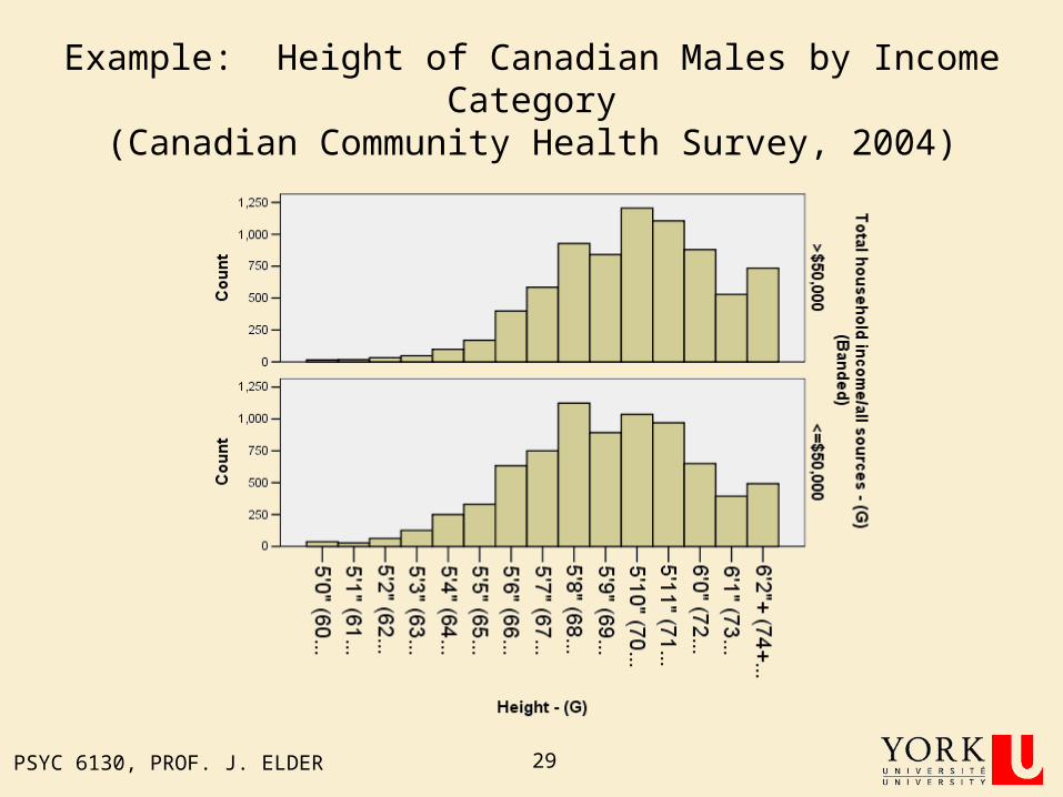
PSYC 6130, PROF. J. ELDER 29
Example: Height of Canadian Males by Income Category(Canadian Community Health Survey, 2004)
PSYC 6130, PROF. J. ELDER 30
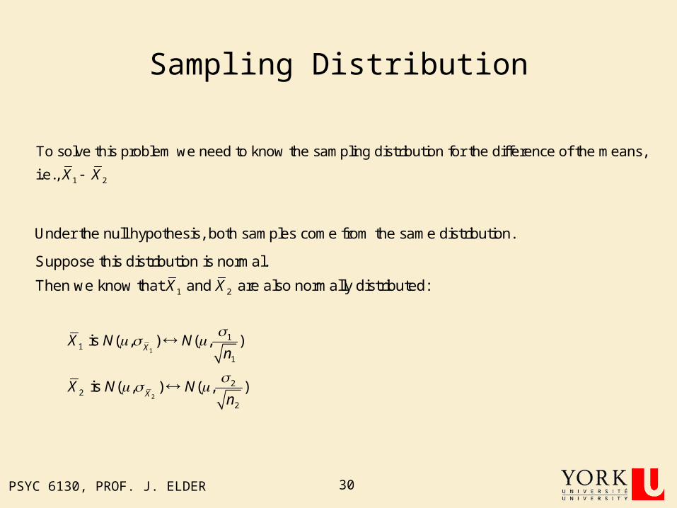
Sampling Distribution
1 2
To solve this problem we need to know the sampling distribution for the difference of the means,
i.e., X X
Under the null hypothesis, both samples come from the same distribution.
1 2
Suppose this distribution is normal.
Then we know that and are also normally distributed:X X
1
2
11
1
22
2
is ( , ) ( , )
is ( , ) ( , )
X
X
X N Nn
X N Nn
PSYC 6130, PROF. J. ELDER 31
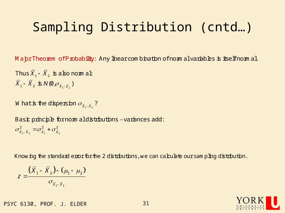
Sampling Distribution (cntd…)
Any linear combination of normalMajor Theorem variables is o if Pr tselobab f noi rlity: mal.
1 2
1 2
1 2
Thus is also normal:
is (0, )X X
X X
X X N
1 2What is the dispersion ?
X X
1 2 1 2
2 2 2
Basic principle for normal distributions - variances add:
X X X X
Knowing the standard error for the 2 distributions, we can calculate our sampling distribution.
1 2
1 2 1 2
X X
X Xz

PSYC 6130, PROF. J. ELDER 32
NHT for Two Large Samples
1 1
2 2
2 2
2 2
If sample is large (e.g., 100), can approximate population variance by sample vR ariancec eal :l:
X X
X X
n
s
s
1 2 1 2
2 2 2And thus we can estimate X X X X
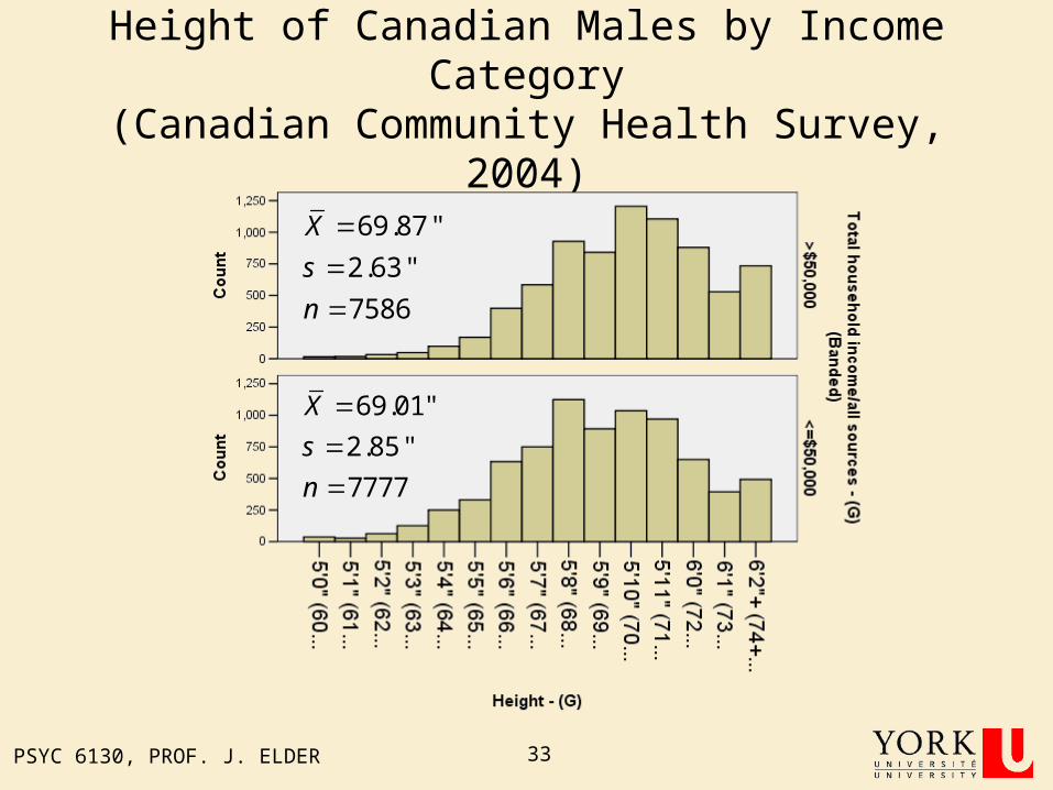
PSYC 6130, PROF. J. ELDER 33
Height of Canadian Males by Income Category(Canadian Community Health Survey, 2004)
69.01"
2.85"
7777
X
s
n
69.87"
2.63"
7586
X
s
n
NHT for Two Small Samples
PSYC 6130, PROF. J. ELDER 35
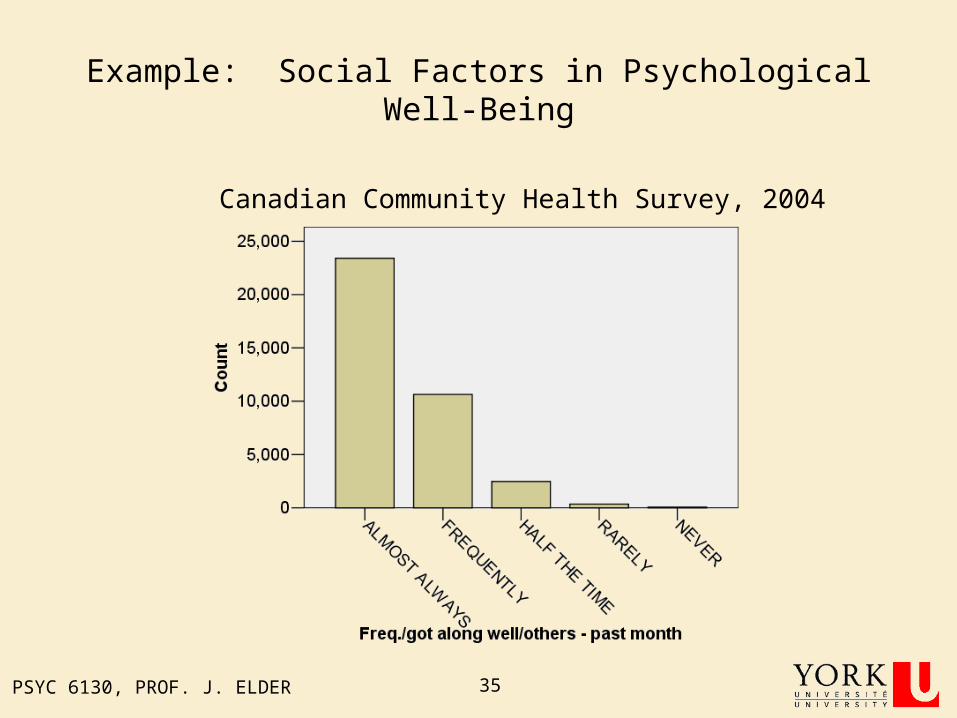
Example: Social Factors in Psychological Well-Being
Canadian Community Health Survey, 2004
PSYC 6130, PROF. J. ELDER 36
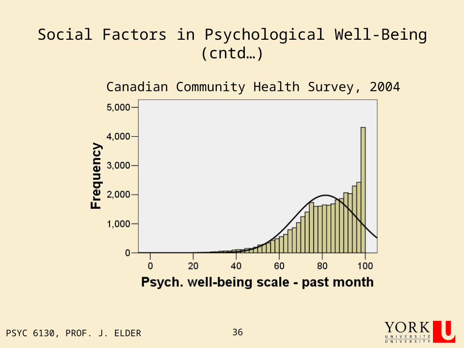
Social Factors in Psychological Well-Being (cntd…)
Canadian Community Health Survey, 2004

PSYC 6130, PROF. J. ELDER 37
Social Factors in Psychological Well-Being (cntd…)
Canadian Community Health Survey, 2004:Respondents who report never getting along with others
PSYC 6130, PROF. J. ELDER 38
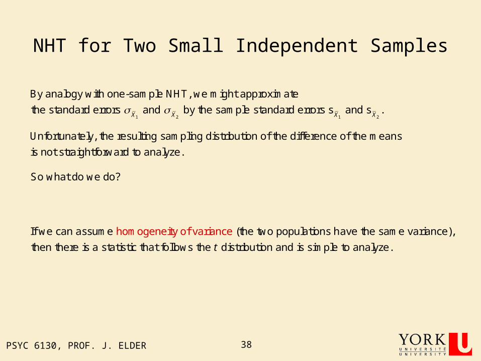
NHT for Two Small Independent Samples
1 2 1 2
By analogy with one-sample NHT, we might approximate
the standard errors and by the sample standard errors s and s .X X X X
Unfortunately, the resulting sampling distribution of the difference of the means
is not straightforward to analyze.
So what do we do?
If we can assume (the two populations have the same variance),
then there is a statistic that follows the distribution an
homogeneit
d is simpl
y of
e to
var
ana
ia
l
nce
yze.t

PSYC 6130, PROF. J. ELDER 39
NHT for Two Small Independent Samples (cntd…)
If both populations have the same variance, we want to use both samples simultaneously
to get the best possible estimate of this variance.
2In general, recall that 1
SSs
n
2 2
1 1 2 22 1 2
1 2 1 2
pooled varia1 1
Thus our formula for the is 1 1 1
nce1p
n s n sSS SSs
n n n n
1 2
2 22
1 2
And the sample standard error is p p
X X
s ss
n n
1 2
1 2 1 2
1 2and follows a distribution with 2 degrees of freedom.X X
X Xt t n n
s
PSYC 6130, PROF. J. ELDER 40
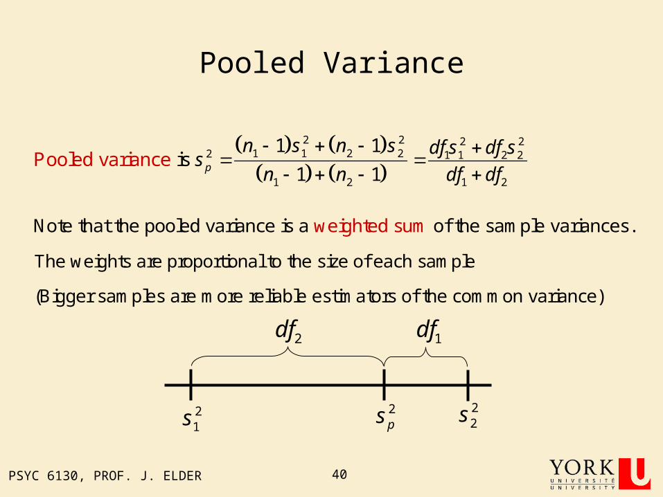
Pooled Variance
2 2 2 21 1 2 22 1 1 2 2
1 2 1 2
1 1ooled variance is
1P
1p
n s n s df s df ss
n n df df
weiNot ghte that ed sum the pooled variance is a of the sample varian ces.
The weights are proportional to the size of each sample
(Bigger samples are more reliable estimators of the common variance)
21s
22s2
ps
1df2df

PSYC 6130, PROF. J. ELDER 41
Social Factors in Psychological Well-Being (cntd…)
Canadian Community Health Survey, 2004:Respondents who report never getting along with others
41.84
23.87
25
X
s
n
36.59
22.40
37
X
s
n
PSYC 6130, PROF. J. ELDER 42
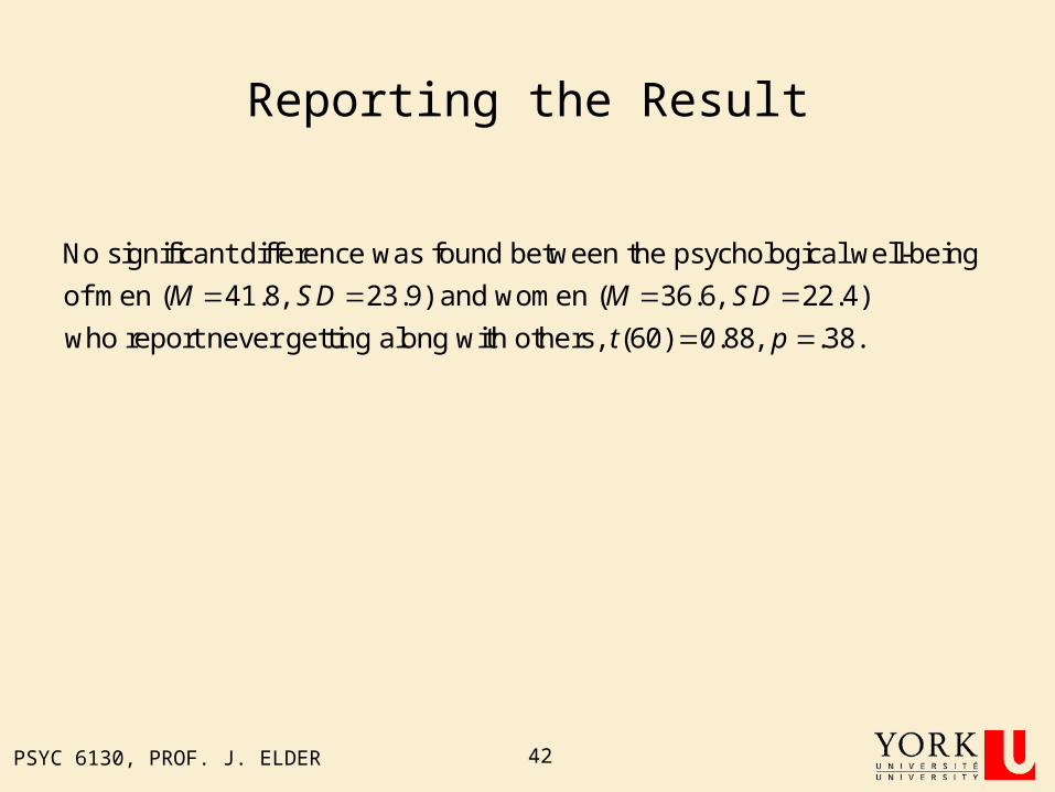
Reporting the Result
No significant difference was found between the psychological well-being
of men ( 41.8, 23.9) and women ( 36.6, 22.4)
who report never getting along with others, (60) 0.88, .38.
M SD M SD
t p

PSYC 6130, PROF. J. ELDER 43
Confidence Intervals for the Difference Between Two Means
1 2
1 2
1 2 1 2
1 2 1 2 X X
X X
X Xt X X ts
s
1 21 2 1 2 crit X XX X t s
1 2( )p
1 2X X
1 2X Xs
.025p .025p95% Confidence Interval
.025t .025t

PSYC 6130, PROF. J. ELDER 44
Underlying Assumptions
• Dependent variable measured on interval or ratio scale.
• Independent random sampling
– (independence within and between samples)
– In experimental work, often make do with random assignment.
• Normal distributions
– Moderate deviations ok due to CLT.
• Homogeneity of Variance
– Only critical when sample sizes are small and different.

End of Lecture 5
Oct 15, 2008
PSYC 6130, PROF. J. ELDER 46
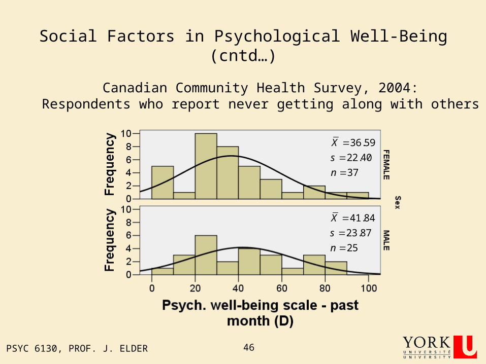
Social Factors in Psychological Well-Being (cntd…)
Canadian Community Health Survey, 2004:Respondents who report never getting along with others
41.84
23.87
25
X
s
n
36.59
22.40
37
X
s
n
PSYC 6130, PROF. J. ELDER 47
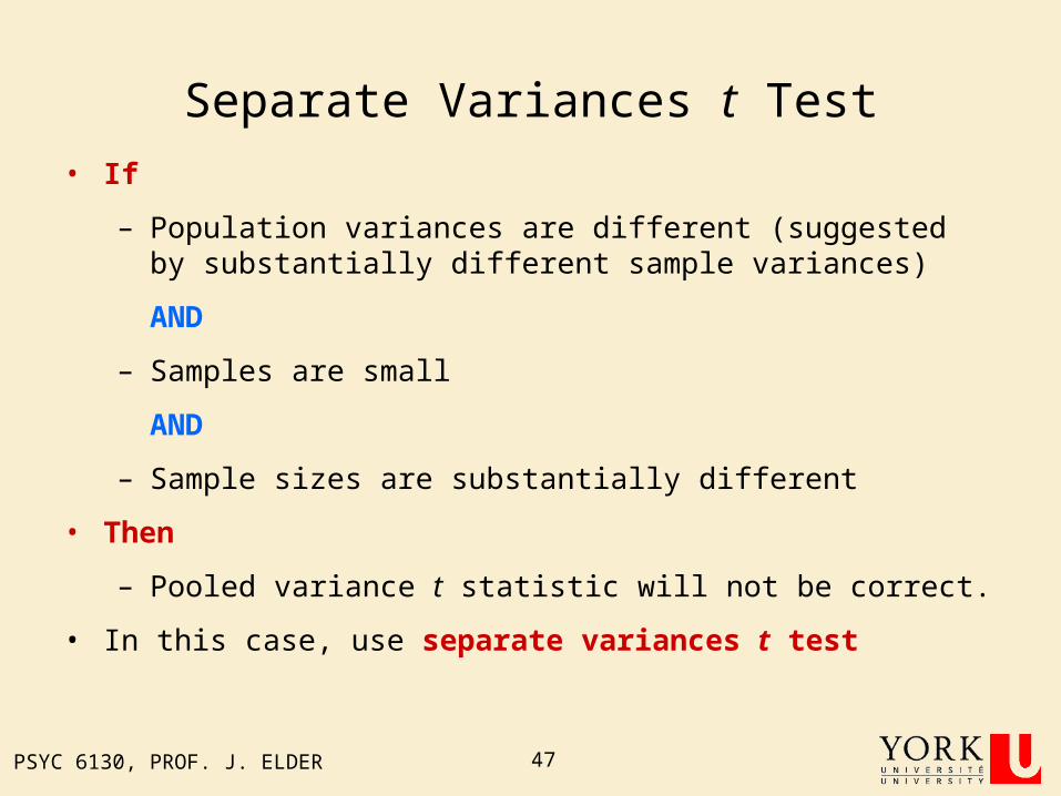
Separate Variances t Test• If
– Population variances are different (suggested by substantially different sample variances)
AND
– Samples are small
AND
– Sample sizes are substantially different
• Then
– Pooled variance t statistic will not be correct.
• In this case, use separate variances t test
PSYC 6130, PROF. J. ELDER 48
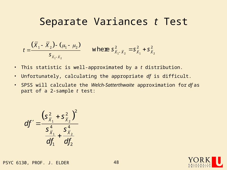
Separate Variances t Test
1 2 1 2
2 2 2where X X X X
s s s 1 2
1 2 1 2
X X
X Xt
s
• This statistic is well-approximated by a t distribution.
• Unfortunately, calculating the appropriate df is difficult.
• SPSS will calculate the Welch-Satterthwaite approximation for df as part of a 2-sample t test:
1 2
1 2
22 2
4 4
1 2
X X
X X
s sdf
s s
df df

PSYC 6130, PROF. J. ELDER 49
Social Factors in Psychological Well-Being (cntd…)
Canadian Community Health Survey, 2004:Respondents who report never getting along with others
41.84
23.87
25
X
s
n
36.59
22.40
37
X
s
n
PSYC 6130, PROF. J. ELDER 50
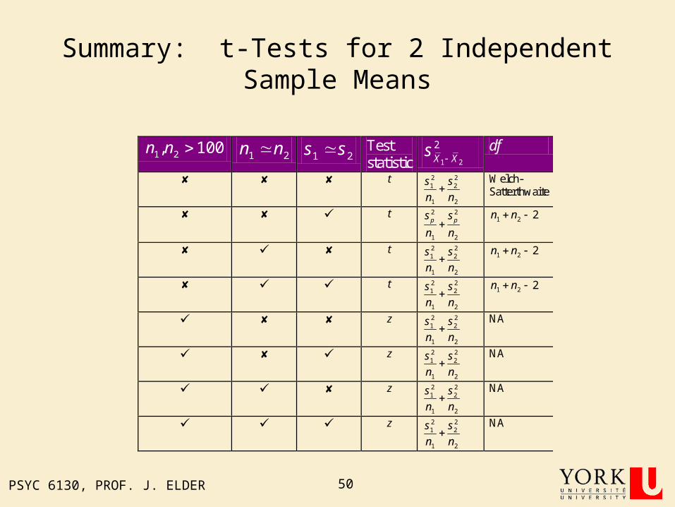
Summary: t-Tests for 2 Independent Sample Means
1 2, 100n n 1 2n n 1 2s s Test statistic 1 2
2X X
s df
t 2 21 2
1 2
s s
n n
Welch-Satterthwaite
t 2 2
1 2
p ps s
n n
1 2 2n n
t 2 21 2
1 2
s s
n n 1 2 2n n
t 2 21 2
1 2
s s
n n 1 2 2n n
z 2 21 2
1 2
s s
n n
NA
z 2 21 2
1 2
s s
n n
NA
z 2 21 2
1 2
s s
n n
NA
z 2 21 2
1 2
s s
n n
NA

PSYC 6130, PROF. J. ELDER 51
More on Homogeneity of Variance• How do we decide if two sample variances are different enough to
suggest different population variances?
• Need NHT for homogeneity of variance.
– F-test
• Straightforward
• Sensitive to deviations from normality
– Levene’s test
• More robust to deviations from normality
• Computed by SPSS

PSYC 6130, PROF. J. ELDER 52
Levene’s Test: Basic Idea
1 21. Replace each score , with its absolute deviation from the sample mean:i iX X
1 1 1
2 2 2
| |
| |
i i
i i
d X X
d X X
1 22. Now run an independent samples t-test on and :i id d
1 2
1 2
d d
d dt
s
SPSS reports an F-statistic for Levene’s test
• Allows the homogeneity of variance for two or more variables to be tested.
• We will introduce the F distribution later in the term.
The Matched t Test

PSYC 6130, PROF. J. ELDER 54
Independent or Matched?
• Application of the Independent-Groups t test depended on independence both within and between groups.
• There are many cases where it is wise, convenient or necessary to use a matched design, in which there is a 1:1 correspondence between scores in the two samples.
• In this case, you cannot assume independence between samples!
• Examples:
– Repeated-subject designs (same subjects in both samples).
– Matched-pairs designs (attempt to match possibly important attributes of subjects in two samples)

PSYC 6130, PROF. J. ELDER 55
Example: Assignment Marks
A3 A472 8070 8069 9383 8888 9388 9387 8888 9385 10085 10070 8072 9060 8083 7581 8368 7536 9380 10065 8365 8341 7573 8868 75
Mean 73 86SD 14 8n 23 23
These scores are not independent!
40
50
60
70
80
90
100
40 60 80 100
Assignment 1 Mark (%)
Ass
ignm
ent
2 M
ark
(%)
PSYC 6130, PROF. J. ELDER 56
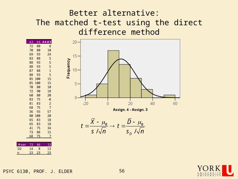
Better alternative: The matched t-test using the direct difference method
A3 A4 A4-A3
72 80 870 80 1069 93 2483 88 588 93 588 93 587 88 188 93 585 100 1585 100 1570 80 1072 90 1860 80 2083 75 -881 83 268 75 736 93 5780 100 2065 83 1865 83 1841 75 3473 88 1568 75 7
Mean 73 86 13SD 14 8 13n 23 23 23
0 0
/ /D
X Dt t
s n s n

PSYC 6130, PROF. J. ELDER 57
Matched vs Independent t-test
• Why does a matched t-test yield a higher t-score than an independent t-test in this example?
– The t-score is determined by the ratio of the difference between the groups and the variance within the groups.
– The matched t-test factors out the portion of the within-group variance due to differences between individuals.
PSYC 6130, PROF. J. ELDER 58
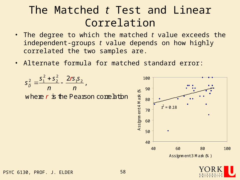
The Matched t Test and Linear Correlation
• The degree to which the matched t value exceeds the independent-groups t value depends on how highly correlated the two samples are.
• Alternate formula for matched standard error:
2 22 1 2 1 22
,
where is the Pearson correlation
D
r
r
s s s ss
n n
r2 = 0.18
40
50
60
70
80
90
100
40 60 80 100
Assignment 3 Mark (%)
Ass
ign
me
nt
4 M
ark
(%
)

PSYC 6130, PROF. J. ELDER 59
Case 1: r = 0
• Independent t-test • Matched t-test
2 22 1 2 1 2
2 21 2
2
1
D
s s s ss
n n
sn
r
s
1 2
2 2 21 2
1X X
s s sn
Thus the t-score will be the same.
2( 1)df n 1df n
Thus the critical t-values will be larger for the matched test.
But note that
PSYC 6130, PROF. J. ELDER 60
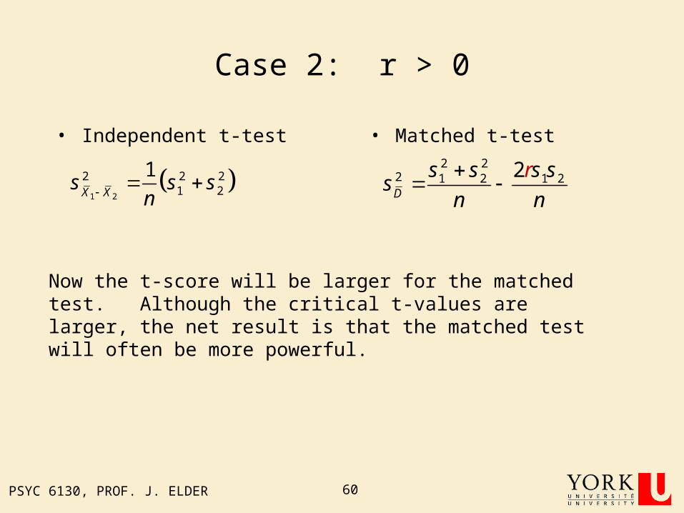
Case 2: r > 0
• Independent t-test • Matched t-test2 2
2 1 2 1 22D
s s s ss
n
r
n
1 2
2 2 21 2
1X X
s s sn
Now the t-score will be larger for the matched test. Although the critical t-values are larger, the net result is that the matched test will often be more powerful.
PSYC 6130, PROF. J. ELDER 61
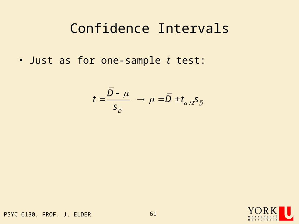
Confidence Intervals
• Just as for one-sample t test:
/ 2 D
D
Dt D t s
s

PSYC 6130, PROF. J. ELDER 62
Repeated Measures Designs
• Many matched sample designs involve repeated measures of the same individuals.
• This can result in carry-over effects, including learning and fatigue.
• These effects can be minimized by counter-balancing the ordering of conditions across participants.

PSYC 6130, PROF. J. ELDER 63
Assumptions of the Matched t Test
• Normality
• Independent random sampling (within samples)