tawit chitsomboon - eng.sut.ac.th
TRANSCRIPT


Editor
Tawit Chitsomboon
International Advisory Board
Adrian Bejan, Duke University, USA Chairman
Jens N. Sørensen, Technical University of Denmark, Denmark Member
Withaya Yongchareon, Chulalongkorn University, Thailand Member
Sylvie Lorente, National Institute of Applied Sciences, France Member
Editorial Board
Mongkol Mongkolwongrojn
Phadungsak Rattanadecho
Pongjate Promwong
Somchai Wongwises
Somnuek Theerakoolphisoot
Sujin Bureerat
Sumrerng Jugjai
Tanongkiat Kiatsiriroat
Worawut Wisutmethangoon
Assistants to the Editor
Atit Koonsrisuk
Chalothorn Thumthae
Published in Thailand by
Journal of Research and Applications in Mechanical Office
School of Mechanical Engineering, Institute of Engineering
Suranaree University of Technology,
111 University Avenue, Nakhon Ratchasima 30000, Thailand
Tel. 66-44-224410, Fax. 66-44-224613
E-mail : [email protected] Website : http://eng.sut.ac.th/me/JRME
ISSN 2229-2152

Letter from the Editor
Dear Fellow Mechanical Engineers,
The academic conferences under the auspice of the Conference of the Mechanical Engineering
Network of Thailand (ME-NETT) have been evolving over the past 25 years with constant progress. I
have observed this progress with impression and admiration; so much so that I had proposed at
several occasions to the Chairs of the various annual Conferences that it is about time that we
establish an academic journal to contribute our academic success to the international community.
In 2009, Dr. Worawut Wisutmethangoon who was the first chairman of TSME (Thai Society of
Mechanical Engineers) gave me the green light to go ahead with the journal. I must accept the guilt
for not being able to push the journal out during that period. Dr. Withaya Yongchareon, the 2nd
Chair
of TSME, continued to urge me to carry on the task that I had proposed. This time around the stress of
the accumulated guilt was beyond a critical limit which made me yield.
The Board of TSME, per my consultation, unanimously agreed that JRAME be an “international” journal publishable in both Thai and English. But for a Thai-language contribution, an English-
language abstract is required.
In addition to our formal aims and scope as indicated on the back page of this publication, we would
very much like to be an alternative force in driving ME-science toward a noble goal. Therefore, we
intend to be very flexible in both coverage and forms. We also intend to be a journal that is “author
friendly.”
Contributing authors to JRAME may choose a referencing format of their choice (either Harvard style
or numbering style or any other style). A paper that is valuable to ME-science will not be denied on
the grounds of its format or its referencing style.
Outcomes of research, applications as well as well thought out “concepts” relating to ME-science in
all perspectives are solicited while subject to the consideration of the editorial board and peer reviews
before they are accepted for publication in JRAME.
In this inaugurating publication, the contributing papers came from two sources as suggested by
TSME board: the best papers awarded in the 24th ME-NETT meeting (marked by asterisks) and the
papers from the 1st International Conference on Mechanical Engineering (ICoME) which were
deemed as appropriate by the Editorial Board. All papers were subject to the authors’ consents as well
as peer reviews.
Like a small gear in an auxiliary equipment, I hope that JRAME will do its part to help drive a very
complicated ME mechanism toward a desirable goal that enriches ourselves, Thailand and the
international community as a whole.
Sincerely,
Tawit Chitsomboon
N.B. We suggest that JRAME be pronounced easily as J-Ra-Me.

Letter of Congratulation
On the occasion of the birth of the Journal of Research and Applications in Mechanical Engineering, I
offer my sincere wishes of success to the editors and all my colleagues in the international research
community who will contribute to this journal.
I am sure that the vibrant scientific life of Thai universities will contribute greatly to its success. In
turn, this new journal will enhance the scientific life and reputation of Thai academia.
Sincerely,
Adrian Bejan
J. A. Jones Distinguished Professor
of Mechanical Engineering, Duke University, USA
Chairman of International Advisory Board, JRAME
*Corresponding Author: E-mail: [email protected]
Vol. 1 No.1 TSME | Journal of Research and Applications in Mechanical Engineering
Enhancement of Thermal Conductivity with Al2O3 for Nanofluids
Apichai Jomphoak1, 2,*, Thitima Maturos1, Tawee Pogfay1, Chanpen Karuwan1, Adisorn Tuantranont1
and Thawatchai Onjun2
1National Electronics and Computer Technology Center (NECTEC), 112 Thailand Science Park, Pathumthani 12120 2Sirindhorn International Institute of Technology, Thammasat University, Pathumthani 12120
Abstract
The enhancement of the thermal conductivity of water in the presence of Alumina (Al2O3) using the employed surfactant,
as the dispersant, is presented in this study. The volume concentration of Alumina–water nanofluids is below 0.2 vol.%. With the
addition of dispersant and surfactant, the thermal conductivity of the produced nanofluids reveals a time-dependent characteristic.
The thermal conductivity, considerably steady at the starting point of measurement, increases gradually with elapsed time. The
results indicate that Alumina–water nanofluids with low concentration of nanoparticles have noticeably higher thermal
conductivities than the water-base fluid without Alumina. For Al2O3 nanoparticles at a volume fraction of 0.001 (0.1 vol.%),
thermal conductivity was enhanced by up to 18.4%.
Keywords: Alumina, Nanofluids, Thermal Conductivity, TPS, Sensor
1. Introduction
The thermal conductivity of thermofluid plays a
significant role in the development of energy-efficient
heat transfer equipment. Passive enhancement methods
are commonly utilized in the electronics, HVAC&R, and
transportation devices. However, the thermal
conductivities of the working fluids such as ethylene
glycol, water, and engine oil are relatively lower than
those of solid particles. In this regard, the development of
advanced heat transfer fluids with higher thermal
conductivity is thus in a strong demand. Nanoparticle
technology is of considerable interest for a large number
of practical applications. A new approach to
nanoparticles in nanofluid was proposed by Dr. Choi at
the USAs Argonne National Laboratory in 1995 [1]. A
number of research works and development focusing on
nanofluids have been recently conducted [2–6]. More
recently, the chemical approach using wet chemistry has
emerged as a powerful method for growing
nanostructures of metals, inorganic semiconductors,
organic materials, and organic–inorganic hybrid systems.
The advantage offered by nanochemistry is that surface
functionalized nanoparticles of metals or dispersible in a
variety of media such as water can be readily prepared.
Furthermore, nanochemistry also lends itself to a precise
control of conditions to produce monodispersed
nanostructures [12].
Alumina nanoparticles are of great interest because
of their use as coolant and application in heat exchanger.
The synthesis methods for Al2O3 nanomaterials include
physical method and chemical method. The physical
method used for Al2O3 nanofluids has been reported
[2,3]. Nanofluids consisting of Al2O3 nanoparticles
directly dispersed in water have been observed to exhibit
significantly improved thermal conductivity
enhancements when compared with nonparticle-
containing fluids or nanofluids containing oxide particles
[3]. Many studies on the thermal conductivities of
nanofluids focused on the nanofluids synthesized via
two-step method. Recently, our study has also
investigated the results of Al2O3–water nanofluids based
on this method [6], and the thermal conductivities of the
Al2O3 suspensions are measured by a transient planar
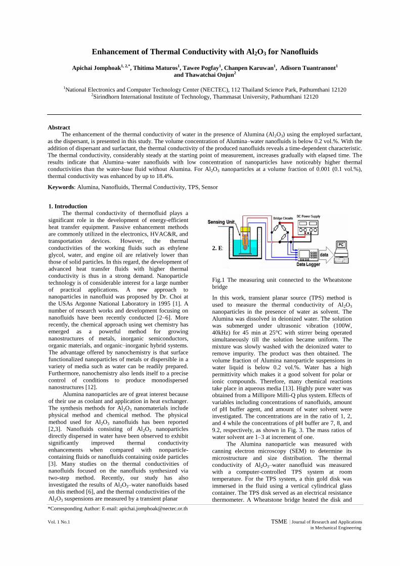
2. Experiments
Fig.1 The measuring unit connected to the Wheatstone
bridge
In this work, transient planar source (TPS) method is
used to measure the thermal conductivity of Al2O3
nanoparticles in the presence of water as solvent. The
Alumina was dissolved in deionized water. The solution
was submerged under ultrasonic vibration (100W,
40kHz) for 45 min at 25°C with stirrer being operated
simultaneously till the solution became uniform. The
mixture was slowly washed with the deionized water to
remove impurity. The product was then obtained. The
volume fraction of Alumina nanoparticle suspensions in
water liquid is below 0.2 vol.%. Water has a high
permittivity which makes it a good solvent for polar or
ionic compounds. Therefore, many chemical reactions
take place in aqueous media [13]. Highly pure water was
obtained from a Millipore Milli-Q plus system. Effects of
variables including concentrations of nanofluids, amount
of pH buffer agent, and amount of water solvent were
investigated. The concentrations are in the ratio of 1, 2,
and 4 while the concentrations of pH buffer are 7, 8, and
9.2, respectively, as shown in Fig. 3. The mass ratios of
water solvent are 1–3 at increment of one.
The Alumina nanoparticle was measured with
canning electron microscopy (SEM) to determine its
microstructure and size distribution. The thermal
conductivity of Al2O3–water nanofluid was measured
with a computer-controlled TPS system at room
temperature. For the TPS system, a thin gold disk was
immersed in the fluid using a vertical cylindrical glass
container. The TPS disk served as an electrical resistance
thermometer. A Wheatstone bridge heated the disk and
JRAME Enhancement of Thermal Conductivity with Al2O3 for Nanofluids
4
simultaneously measured its resistance. The electrical
resistance of the gold disk varies in proportion to changes
in temperature as shown in Fig. 1. The thermal
conductivity was then estimated from Fourier’s law. The
transient TPS system was calibrated with the deionized
water at room temperature. The Al2O3–water nanofluids
were filled into the glass container to measure the
thermal conductivity. The inner diameter and length of
long glass container are 19 mm and 240 mm,
respectively. A time sequence of thermal conductivity
measurement of the Alumina nanofluids was conducted
at intervals of 1–5 min. The measurement ended up at 30
min when there was no apparent change in the thermal
conductivity. The time profile of the thermal conductivity
distribution of the Alumina nanofluids then can be
examined.
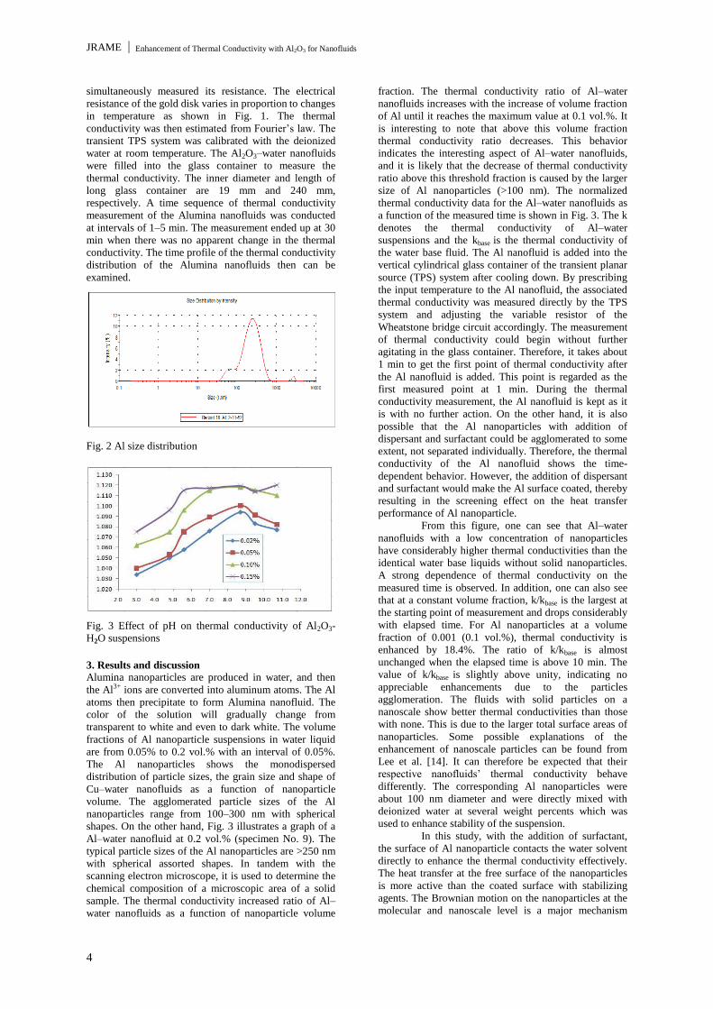
Fig. 2 Al size distribution
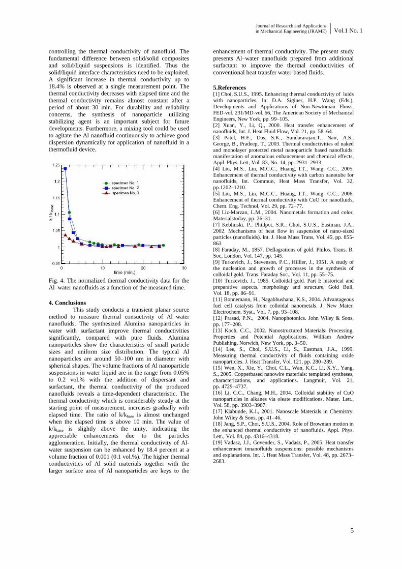
Fig. 3 Effect of pH on thermal conductivity of Al2O3-
H2O suspensions
3. Results and discussion
Alumina nanoparticles are produced in water, and then
the Al3+ ions are converted into aluminum atoms. The Al
atoms then precipitate to form Alumina nanofluid. The
color of the solution will gradually change from
transparent to white and even to dark white. The volume
fractions of Al nanoparticle suspensions in water liquid
are from 0.05% to 0.2 vol.% with an interval of 0.05%.
The Al nanoparticles shows the monodispersed
distribution of particle sizes, the grain size and shape of
Cu–water nanofluids as a function of nanoparticle
volume. The agglomerated particle sizes of the Al
nanoparticles range from 100–300 nm with spherical
shapes. On the other hand, Fig. 3 illustrates a graph of a
Al–water nanofluid at 0.2 vol.% (specimen No. 9). The
typical particle sizes of the Al nanoparticles are >250 nm
with spherical assorted shapes. In tandem with the
scanning electron microscope, it is used to determine the
chemical composition of a microscopic area of a solid
sample. The thermal conductivity increased ratio of Al–
water nanofluids as a function of nanoparticle volume
fraction. The thermal conductivity ratio of Al–water
nanofluids increases with the increase of volume fraction
of Al until it reaches the maximum value at 0.1 vol.%. It
is interesting to note that above this volume fraction
thermal conductivity ratio decreases. This behavior
indicates the interesting aspect of Al–water nanofluids,
and it is likely that the decrease of thermal conductivity
ratio above this threshold fraction is caused by the larger
size of Al nanoparticles (>100 nm). The normalized
thermal conductivity data for the Al–water nanofluids as
a function of the measured time is shown in Fig. 3. The k
denotes the thermal conductivity of Al–water
suspensions and the kbase is the thermal conductivity of
the water base fluid. The Al nanofluid is added into the
vertical cylindrical glass container of the transient planar
source (TPS) system after cooling down. By prescribing
the input temperature to the Al nanofluid, the associated
thermal conductivity was measured directly by the TPS
system and adjusting the variable resistor of the
Wheatstone bridge circuit accordingly. The measurement
of thermal conductivity could begin without further
agitating in the glass container. Therefore, it takes about
1 min to get the first point of thermal conductivity after
the Al nanofluid is added. This point is regarded as the
first measured point at 1 min. During the thermal
conductivity measurement, the Al nanofluid is kept as it
is with no further action. On the other hand, it is also
possible that the Al nanoparticles with addition of
dispersant and surfactant could be agglomerated to some
extent, not separated individually. Therefore, the thermal
conductivity of the Al nanofluid shows the time-
dependent behavior. However, the addition of dispersant
and surfactant would make the Al surface coated, thereby
resulting in the screening effect on the heat transfer
performance of Al nanoparticle.
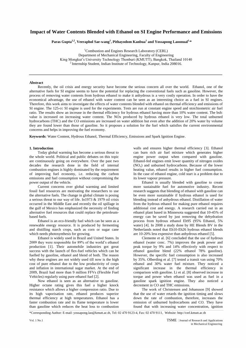
From this figure, one can see that Al–water
nanofluids with a low concentration of nanoparticles
have considerably higher thermal conductivities than the
identical water base liquids without solid nanoparticles.
A strong dependence of thermal conductivity on the
measured time is observed. In addition, one can also see
that at a constant volume fraction, k/kbase is the largest at
the starting point of measurement and drops considerably
with elapsed time. For Al nanoparticles at a volume
fraction of 0.001 (0.1 vol.%), thermal conductivity is
enhanced by 18.4%. The ratio of k/kbase is almost
unchanged when the elapsed time is above 10 min. The
value of k/kbase is slightly above unity, indicating no
appreciable enhancements due to the particles
agglomeration. The fluids with solid particles on a
nanoscale show better thermal conductivities than those
with none. This is due to the larger total surface areas of
nanoparticles. Some possible explanations of the
enhancement of nanoscale particles can be found from
Lee et al. [14]. It can therefore be expected that their
respective nanofluids’ thermal conductivity behave
differently. The corresponding Al nanoparticles were
about 100 nm diameter and were directly mixed with
deionized water at several weight percents which was
used to enhance stability of the suspension.
In this study, with the addition of surfactant,
the surface of Al nanoparticle contacts the water solvent
directly to enhance the thermal conductivity effectively.
The heat transfer at the free surface of the nanoparticles
is more active than the coated surface with stabilizing
agents. The Brownian motion on the nanoparticles at the
molecular and nanoscale level is a major mechanism
Journal of Research and Applications
in Mechanical Engineering (JRAME) Vol.1 No. 1
5
controlling the thermal conductivity of nanofluid. The
fundamental difference between solid/solid composites
and solid/liquid suspensions is identified. Thus the
solid/liquid interface characteristics need to be exploited.
A significant increase in thermal conductivity up to
18.4% is observed at a single measurement point. The
thermal conductivity decreases with elapsed time and the
thermal conductivity remains almost constant after a
period of about 30 min. For durability and reliability
concerns, the synthesis of nanoparticle utilizing
stabilizing agent is an important subject for future
developments. Furthermore, a mixing tool could be used
to agitate the Al nanofluid continuously to achieve good
dispersion dynamically for application of nanofluid in a
thermofluid device.
Fig. 4. The normalized thermal conductivity data for the
Al–water nanofluids as a function of the measured time.
4. Conclusions
This study conducts a transient planar source
method to measure thermal consuctivity of Al–water
nanofluids. The synthesized Alumina nanoparticles in
water with surfactant improve thermal conductivities
significantly, compared with pure fluids. Alumina
nanoparticles show the characteristics of small particle
sizes and uniform size distribution. The typical Al
nanoparticles are around 50–100 nm in diameter with
spherical shapes. The volume fractions of Al nanoparticle
suspensions in water liquid are in the range from 0.05%
to 0.2 vol.% with the addition of dispersant and
surfactant, the thermal conductivity of the produced
nanofluids reveals a time-dependent characteristic. The
thermal conductivity which is considerably steady at the
starting point of measurement, increases gradually with
elapsed time. The ratio of k/kbase is almost unchanged
when the elapsed time is above 10 min. The value of
k/kbase is slightly above the unity, indicating the
appreciable enhancements due to the particles
agglomeration. Initially, the thermal conductivity of Al-
water suspension can be enhanced by 18.4 percent at a
volume fraction of 0.001 (0.1 vol.%). The higher thermal
conductivities of Al solid materials together with the
larger surface area of Al nanoparticles are keys to the
enhancement of thermal conductivity. The present study
presents Al–water nanofluids prepared from additional
surfactant to improve the thermal conductivities of
conventional heat transfer water-based fluids.
5.References [1] Choi, S.U.S., 1995. Enhancing thermal conductivity of luids
with nanoparticles. In: D.A. Siginer, H.P. Wang (Eds.),
Developments and Applications of Non-Newtonian Flows, FED-vol. 231/MD-vol. 66, The American Society of Mechanical
Engineers, New York, pp. 99–105.
[2] Xuan, Y., Li, Q., 2000. Heat transfer enhancement of nanofluids, Int. J. Heat Fluid Flow, Vol. 21, pp. 58–64.
[3] Patel, H.E., Das, S.K., Sundararajan,T., Nair, A.S., George, B., Pradeep, T., 2003. Thermal conductivities of naked
and monolayer protected metal nanoparticle based nanofluids:
manifestation of anomalous enhancement and chemical effects, Appl. Phys. Lett, Vol. 83, No. 14, pp. 2931–2933.
[4] Liu, M.S., Lin, M.C.C., Huang, I.T., Wang, C.C., 2005.
Enhancement of thermal conductivity with carbon nanotube for nanofluids, Int. Commun, Heat Mass Transfer, Vol. 32,
pp.1202–1210.
[5] Liu, M.S., Lin, M.C.C., Huang, I.T., Wang, C.C., 2006. Enhancement of thermal conductivity with CuO for nanofluids,
Chem. Eng. Technol, Vol. 29, pp. 72–77.
[6] Liz-Marzan, L.M., 2004. Nanometals formation and color, Materialstoday, pp. 26–31.
[7] Keblinski, P., Phillpot, S.R., Choi, S.U.S., Eastman, J.A.,
2002. Mechanisms of heat flow in suspension of nano-sized particles (nanofluids). Int. J. Heat Mass Trans, Vol. 45, pp. 855-
863
[8] Faraday, M., 1857. Deflagrations of gold. Philos. Trans. R. Soc, London, Vol. 147, pp. 145.
[9] Turkevich, J., Stevenson, P.C., Hillier, J., 1951. A study of
the nucleation and growth of processes in the synthesis of colloidal gold. Trans. Faraday Soc., Vol. 11, pp. 55–75.
[10] Turkevich, J., 1985. Colloidal gold. Part I: historical and
preparative aspects, morphology and structure, Gold Bull, Vol. 18, pp. 86–91.
[11] Bonnemann, H., Nagabhushana, K.S., 2004. Advantageous
fuel cell catalysts from colloidal nanometals. J. New Mater. Electrochem. Syst., Vol. 7, pp. 93–108.
[12] Prasad, P.N., 2004. Nanophotonics. John Wiley & Sons,
pp. 177–208. [13] Koch, C.C., 2002. Nanostructured Materials: Processing,
Properties and Potential Applications. William Andrew
Publishing, Norwich, New York, pp. 3–50. [14] Lee, S., Choi, S.U.S., Li, S., Eastman, J.A., 1999.
Measuring thermal conductivity of fluids containing oxide
nanoparticles. J. Heat Transfer, Vol. 121, pp. 280–289. [15] Wen, X., Xie, Y., Choi, C.L., Wan, K.C., Li, X.Y., Yang,
S., 2005. Copperbased nanowire materials: templated syntheses,
characterizations, and applications. Langmuir, Vol. 21, pp. 4729–4737.
[16] Li, C.C., Chang, M.H., 2004. Colloidal stability of CuO
nanoparticles in alkanes via oleate modifications. Mater. Lett., Vol. 58, pp. 3903–3907.
[17] Klabunde, K.J., 2001. Nanoscale Materials in Chemistry.
John Wiley & Sons, pp. 41–46. [18] Jang, S.P., Choi, S.U.S., 2004. Role of Brownian motion in
the enhanced thermal conductivity of nanofluids. Appl. Phys.
Lett., Vol. 84, pp. 4316–4318. [19] Vadasz, J.J., Govender, S., Vadasz, P., 2005. Heat transfer
enhancement innanofluids suspensions: possible mechanisms
and explanations. Int. J. Heat Mass Transfer, Vol. 48, pp. 2673–2683.
*Corresponding Author: E-mail: [email protected], Tel: 02 470 9123-4, Fax: 02 470 9111, Website: http://cerl.kmutt.ac.th
Vol. 1 No.1 TSME | Journal of Research and Applications in Mechanical Engineering
Impact of Water Contents Blended with Ethanol on SI Engine Performance and Emissions
Paras Gupta1,2, Veeraphol Sae-wang1, Pithayodom Kanbua1 and Yossapong Laoonual1,*
1Combustion and Engines Research Laboratory (CERL)
Department of Mechanical Engineering, Faculty of Engineering
King Mongkut’s University Technology Thonburi (KMUTT), Bangkok, Thailand 10140 2 Internship Student, Indian Institute of Technology, Kanpur, India 208016.
Abstract
Recently, the oil crisis and energy security have become the serious concern all over the world. Ethanol, one of the
alternative fuels for SI engine seems to have the potential for replacing the conventional fuels such as gasoline. However, the
process of removing water contents from hydrous ethanol to make it anhydrous is a very costly operation. In order to have the
economical advantage, the use of ethanol with water content can be seen as an interesting choice as a fuel in SI engines.
Therefore, this work aims to investigate the effects of water contents blended with ethanol on thermal efficiency and emissions of
SI engine. The 125-cc SI engine is used for the experiments. Tests are run at constant engine speed and stoichiometric air fuel
ratio. The results show an increase in the thermal efficiency for hydrous ethanol having more than 10% water content. The bsfc
value is increased on increasing water content. The NOx produced by hydrous ethanol is very low. The total unburned
hydrocarbons (THC) and the CO emissions are increased on water addition but even after the addition of 20% water by volume
they are found lower than those of gasoline. So it proposes a solution for the fuel which satisfies the current environmental
concerns and helps in improving the fuel economy.
Keywords: Water Content, Hydrous Ethanol, Thermal Efficiency, Emissions and Spark Ignition Engine.
1. Introduction
Today global warming has become a serious threat to
the whole world. Political and public debates on this topic
are continuously going on everywhere. Over the past two
decades the research done in the field of internal
combustion engines is highly dominated by the requirement
of improving fuel economy, i.e. reducing the carbon
emissions and fuel consumption without compromising the
power output of the vehicle.
Current concerns over global warming and limited
fossil fuel resources are motivating the researchers to use
the alternative fuels. The change in global climate is posing
a serious threat to our way of life. In1973 & 1979 oil crisis
occurred in the Middle East and recently the oil spillage in
the gulf of Mexico has emphasized the necessity of finding
alternative fuel resources that could replace the petroleum-
based fuels.
Ethanol is an eco-friendly fuel which can be seen as a
renewable energy resource. It is produced by fermenting
and distilling starch crops, such as corn or sugar cane
which needs photosynthesis for growing.
Ethanol is widely used in Brazil and United States. In
2009 they were responsible for 89% of the world’s ethanol
production [1]. Their automobile industries got great
success with the launch of flex-fuel vehicles which can be
fuelled by gasoline, ethanol and blend of both. The reason
why these engines are not widely used till now is the high
cost of pure ethanol due to the low productivity of corps
and inflation in international sugar market. At the end of
2009, Brazil had more than 9 million FFVs (Flexible Fuel
Vehicles) regularly using pure ethanol fuel [2].
Now ethanol is seen as an alternative to gasoline.
Higher octane rating gives this fuel a higher knock
resistance which allows a higher compression ratio. Due to
its high vaporisation rate, ethanol produces superior
thermal efficiency at high temperatures. Ethanol has a
faster combustion rate and its flame temperature is lower
than gasoline which reduces the heat loss to combustion
walls and ensures higher thermal efficiency [3]. Ethanol
can burn rich air fuel mixture which generates higher
engine power output when compared with gasoline.
Ethanol-fed engines emit lower quantity of nitrogen oxides
(NOx) and unburned hydrocarbons. Because of the lower
heating value, ethanol results in higher fuel consumption.
In the case of ethanol engine, cold start is a problem due to
its lower vapour pressure.
Ethanol is usually blended with gasoline to create
more sustainable fuel for automotive industry. Recent
research suggests that blending of ethanol with gasoline can
be even more sustainable if hydrous ethanol is used for
blending instead of anhydrous ethanol. Distillation of water
from the hydrous ethanol for making pure ethanol requires
additional cost and energy. A research carried out in an
ethanol plant based in Minnesota suggested that 10-45% of
energy can be saved by just removing the dehydration
process from hydrous ethanol Eh95 (95% Ethanol, 5%
water) [4]. In 2008 a study done by HE Blends BV in the
Netherlands noted that Eh10-Eh26 hydrous ethanol blends
are 10-20% less expensive than anhydrous ethanol [5].
Clemente et al. [6] concluded that the use of hydrous
ethanol (water conc. 7%) improves the peak power and
peak torque by 9% and 14% effectively with respect to
ethanol gasoline blend (22% ethanol 78% gasoline).
However, the specific fuel consumption is also increased
by 35%. Olberding et al. [7] tested a transit van using 70%
ethanol and 30% water fuel mixture. They noticed a
significant increase in the thermal efficiency in
comparison with gasoline. Li et al. [8] observed increase in
torque and power when ethanol was used as fuel in a
gasoline spark ignition engine. They also noticed a
decrement in CO and THC emissions.
The work of Christensen and Johansson [9] showed
that the use of water retards the ignition timing and slows
down the rate of combustion, therefore, increases the
emission of unburned hydrocarbons and CO. They have
found that with increasing water concentration, ignition

JRAME Impact of Water Contents Blended with Ethanol on Sl Engine Performance and Emissions
8
timing should be advanced to ensure the sufficient
evaporation of water. They observed low NOx emissions
with high water contents because higher latent heat of
vaporization of water causes the reduction in peak cylinder
temperature.
A number of research works have been carried out to
investigate water tolerances of ethanol/gasoline blends and
preventing the phase separation between gasoline and
water(in low ethanol blends) to avoid the corrosion
problem [10] but currently the researchers believe that they
have overlooked the great possibility of using hydrous
ethanol as fuel which is environment friendly as well as
economical.
The aim of the present research is therefore to
investigate the effects of water contents in ethanol on the
performance of a spark ignition engine and compare them
with the gasohol as a fuel. Emissions characteristics are
also compared. Tests are conducted on a one cylinder,
small SI engine with few modifications. This would
determine the possibility of using hydrous ethanol as fuel in
the near future.
2. Experimental Section
2.1 Experiment set up
The experimental work was carried on a Honda
Model Wave-125i engine which was a one cylinder, four
stroke SI engine whose technical specifications are
mentioned in Table
1. The engine was originally designed for gasoline but it
was modified for using hydrous ethanol. The injector size
was increased and fuel injection and ignition timing were
controlled by commercial electronic control unit (ECU).
ECU optimizes the fuel injection period and spark timing to
maintain a constant air fuel ratio and engine revolution
speed. After these modifications, the engine was installed
on an Eddy Current Dynamometer for measuring and
controlling the torque produced by the engine.
Table1. Engine Specifications
Model HONDA WAVE 125i
Engine type 4-stroke single cylinder
Displacement Volume 124.8 cm3
Bore x Stroke 52.4 x 57.9 mm
Compression ratio 9.3:1
Engine speed 1,000-10,000 rpm
Cooling system Forced air
Fuel supply Electrical fuel injection
For measuring the variation of cylinder pressure with crank
angle, a pressure sensor with compatible charge amplifier
and crank shaft angle encoder was used with a high speed
data acquisition system designed on Indiwin software. The
complete data of in-cylinder pressure will not be analysed
here.
In the exhaust stream oxygen sensor was installed
for measuring the equivalence ratio from the exhaust of the
engine. Exhaust system (MRU Model SWG 200-1)
measures and analyzes the exhaust temperature with the
contribution of O2, CO2, CO, NO, NO2, NOx and unburned
hydrocarbons in the exhaust stream. Fuel consumption and
laminar air flow was measured manually using a weight
measuring machine and a U- tube manometer respectively.
The equivalence ratio obtained from the oxygen sensor was
compared with the value calculated from exhaust gas
composition results and intake laminar flow. The schematic
diagram of the experiment is shown in Fig. 1.
Fig. 1 Experimental set up
2.2. Experiment Procedure
Four fuels were considered for the analysis: Gasohol
Octane 91 (E10), Pure Ethanol (E100), Ethanol with 10%
water by volume (Eh90) and Ethanol with 20% water
content (Eh80). The physical and chemical properties of
these fuels are mentioned in Table 2. Ignition timing was
optimized for the maximum torque in each condition. The
test conditions are shown in Table 3.
Table 2. Physical – Chemical properties of the fuels experimented
Parameter Gasohol E10 E100 Eh90 Eh80
Composition(by volume) 90% Gasoline
10% Ethanol
100% Ethanol 90% Ethanol
10% Water
80% Ethanol
20% Water
Density (g/cc) 0.7650 0.7921 0.8291 0.8492
Lower Heating Value(MJ/kg) 41.087 28.865 25.318 24.936
Stoichiometric A/F 14.421 8.953 7.853 7.734
Chemical Structure* C6.66H15.33O0.22 C2H5OH C1.47H4.94O C1.42H4.85O
Carbon Mass(%) 80.89 52.17 45.76 45.07
Hydrogen mass(%) 15.51 13.04 12.80 12.78
Oxygen mass(%) 3.60 34.79 41.44 42.14
*calculated for 1 mole of fuel from the given volume ratio of contents (using measured value of densities and standard
value of molecular weight)

Journal of Research and Applications
in Mechanical Engineering (JRAME) Vol.1 No. 1
9
Table 3. Test Conditions
No. Fuel Load (%) Engine Speed
(rpm) λ
1 E10
25,50,100
5000
1
2 E100
3 Eh90
4 Eh80
Throughout the experiment, the air fuel ratio was kept
constant at its stoichiometric value and engine crank shaft
revolution was maintained at 5000 rpm. The engine load
was varied by the position of throttle. For each test
condition, brake power, indicated power, thermal
efficiency, brake specific fuel consumption and regulated
exhaust emissions were reported. Three load conditions
were tested for each fuel to make the comparison more
reliable. To enhance the accuracy of results and to avoid
the fluctuations in the measured values every test was
carried out until it reached its steady state and the final
value was averaged out over this period.
3. Results and Discussion
The present motive is to observe the changes in brake
power, thermal efficiency, bsfc and regulated emissions
with increasing water content in ethanol and to compare it
with the corresponding gasohol (E10).
3.1. Brake Power
As we can see in Fig. 2, when we switch the fuel
from gasohol to pure ethanol, an increment in brake power
of 12.53%, 4.30% and 4.95% is observed for 25%, 50%
and 100% load respectively. The brake power is directly
proportional to the torque output of crank shaft at constant
engine speed. It is found that the laminar flame speed is
higher in case of ethanol than gasoline [11]. As the engine
speed increases, there is less time available for the
complete combustion, so a higher flame speed is required.
This makes hydrous ethanol produce more torque when
compared with gasoline. This change is enhanced in case
of higher engine speed and reversed in case of lower engine
speed due to the high heating value of gasoline [3]. From
Table 2, it can be observed that gasoline has a higher
heating value than ethanol and it decreases with increasing
water content. It causes a reduction in the brake power with
increasing water contents. 20% water content by volume in
ethanol reduces the brake power 21.74%, 2.55% and 6.42%
from E100 for 25%, 50% and 100% load conditions
respectively.
Fig. 2 Brake Power in case of Gasohol(E10) and ethanol
with 0, 10 and 20% water contents at 5000 rpm and
stoichiometric A/F(λ=1) for 25%, 50% and 100% load
conditions
3.2 Brake specific fuel consumption ( bsfc )
The brake specific fuel consumption is increased
with water content as it can be observed from Fig. 3. All
the tests are operated on stoichiometric condition. The
stoichiometric A/F for gasohol is 14.421 which is
calculated by using the given volume ratio and measured
density values. It is much higher than stoichiometric A/F
for pure ethanol and found decreased as water is added in
the fuel (see Table 2). Therefore, the bsfc value of ethanol
is observed 11.76 %, 39.67 % and 41.90 % higher than that
of gasohol for 25%, 50% and 100% load conditions
respectively. Another reason supporting this trend is the
lower heating value of ethanol with respect to gasoline. As
we mix water in the alcohol, the lower heating value is
decreased; therefore, bsfc value is increased. For Eh80 it
reached 47.88 % of its E100 value at 25% throttle opening.
Therefore hydrous ethanol can improve fuel economy when
compared with gasoline only with proper engine hardware
modifications. This result is consistent with the previous
research done on the similar topics [6&12].
Fig. 3 BSFC in case of Gasohol(E10) and ethanol with 0,
10 and 20% water contents (E100-Eh80) at 5000 rpm and
stoichiometric A/F(λ=1) for 25%, 50% and 100% load
conditions
3.3 Thermal Efficiency
The thermal efficiency in case of ethanol is higher
than that of gasoline. This could be explained by less heat
loss through cylinder walls because of higher laminar flame
speed in case of ethanol. For 25%, 50% and 100% load,
thermal efficiency of E100 is 27.36%, 1.91% and 12.04%
higher than that of gasoline respectively.
It is observed that the efficiency is decreased with
increasing water contents after a small primary stage. It is
expected that during the combustion process water takes
the significant amount of energy, when it converts from
liquid to vapour state which causes the thermal cooling of
charge inside the cylinder. The efficiency in case of Eh80 is
21.75%, 7.22% and 12.82% lower than that in case of E100
for 25%, 50% and 100% load conditions respectively. The
difference between the brake thermal efficiency obtained in
case of gasohol and Eh80 is very low as it can be seen in
Fig. 4. It favours the use of hydrous ethanol containing
more than 10% water instead of gasohol without
compromising the thermal efficiency of engine.

JRAME Impact of Water Contents Blended with Ethanol on Sl Engine Performance and Emissions
10
Fig. 4 Thermal Efficiency in case of Gasohol(E10) and
ethanol with 0, 10 and 20% water contents at 5000 rpm and
stoichiometric A/F(λ=1) for 25%, 50% and 100% load
conditions
3.4 Emissions
3.4 Emissions
Ethanol shows a significant reduction in CO
emissions when compared with gasoline. Due to the
oxygen presence in ethanol, there is a noticeable
conversion of CO into CO2 which causes a decline of
76.24%, 46.09% and 56.20% in CO emissions for 25%,
50% and 100% load respectively when we switch the fuel
from gasohol to pure ethanol. Water content in ethanol
slows down the combustion rate. Therefore, as shown in
Fig. 5(a), it increases the CO emissions from the pure
ethanol values. The CO emission observed in case of Eh 80
is 2.06%, 36.78% and 30.81% higher than that of E100 for
25%, 50% and 100 % throttle opening respectively. From
this result hydrous ethanol comes out as a better
environment friendly fuel considering the adverse effects
caused by CO as pollutants.
NOx emissions highly depend upon the in-cylinder
temperature. These are found decreased linearly with water
addition. The peak pressure inside the cylinder which is
measured by pressure transducer is found to be decreased
with increasing water contents. Because of that, a decrease
in cylinder peak temperature is expected. NOx emissions in
case of Eh80 are 79.18%, 65.25%, 49.04% lower than those
in case of gasohol for 25%, 50% and 100% load conditions
respectively. The linear slow down in NOx can be observed
in Fig. 5(b).
Hydrous ethanol seemed to be a better alternative as
shown by Fig. 5(c) in terms of THC emissions. Using pure
ethanol (E100) a decrement of 56.75%, 50.24% and
58.87% in THC emissions is observed from the gasohol
values for 25%, 50% and 100% load conditions
respectively. One reason is because of the polar character
of ethanol which prevents it from bonding with non-polar
engine oil at surface of cylinder wall [13]. Water content
causes the incomplete combustion responsible for higher
THC values. Eh80 produces higher hydrocarbons than pure
ethanol for all loads.
4. Conclusion
From the results, it can be concluded that the impact
of water content blended with ethanol on the thermal
efficiency of engine limits the amount of water which can
be tolerated with ethanol. The addition of more than 20%
water in ethanol might result in a major loss of efficiency.
The bsfc in case of ethanol is 41.9% higher than that of
gasohol at 100% load. The bsfc is also increased on
increasing water content because of that it produces the
brake power about the same range that can be achieved
using gasohol. The measured brake power is always higher
in case of ethanol when compared with gasohol. The CO
emissions are reduced when ethanol is used in place of
gasohol. CO emissions then increase with increasing water
content at all loads (throttle positions). A significant
reduction in NOx emissions is achieved by blending it with
water. THC emissions increase with water content forcing a
tolerance limit of water in ethanol. Therefore, we can
conclude that using hydrous ethanol definitely has an
economical advantage. The addition of water less than 20%
by volume makes compromise with the engine efficiency
and the emissions produced are still lower than those in
case of gasohol, the commonly used motor fuel in
Thailand.
(a) Carbonmonoxide (CO) emissions
(b) Nitric oxide (NOx) emissions
(c) Total Unburned Hydrocarbon (THC) emissions
Fig. 5 CO, NOX and THC emissions from Gasohol (E10)
and ethanol 0, 10 and 20% water contents at 5000 rpm and
stoichiometric A/F for 25%, 50% and 100% load
conditions.
5. Acknowledgements
The authors would like to thank, Junior Science
Talent Project (JSTP), National Science and Technology
Department Agency (NSTDA), Thailand for providing
financial supports of Veeraphol’s research project. Special
thanks also go to all CERL members who gave us
assistance many occasions.
6. References [1] Renewable Fuels Association. 2010. 2010 Ethanol Industry Outlook, Climate of Opportunity. (cited 12 Sep 2010). Available
from : URL: http://www.ethanolrfa.org/page/objects/pdf/outlook-
/RFAoutlook2010_fin.pdf?nocdn=1. [2] Associação Nacional dos Fabricantesmde Veículos
Automotores- ANFAVEA. 2009. Brazilian Automotive Industry
Yearbook 2009, Chapter 2 Vehicles-production, domestic sales and exports. (cited 12 Sep 2010). Available from : URL:
http://www.anfavea.com.br/anuario2009/-capitulo2a.pdf.

Journal of Research and Applications
in Mechanical Engineering (JRAME) Vol.1 No. 1
11
[3] Costa, R.C., Sodre, J.R., 2009. Hydrous ethanol vs. gasoline-ethanol blend: Engine performance and emissions. Fuel, Vol. 89,
No. 2, pp. 287-293.
[4] Kortba, R., 2008. Testing the Water. Ethanol Producer Magazine. (cited 12 Sep 2010). Available from : URL:
http://www.ethanolproducer.com/article.jsp?article_id=3981&q=&
page=1. [5] Jager, D.E., Visser R., 2007. Hydrous Ethanol: Cheap and
Sustainable. In: Proceedings of the Connecting Clean Mobility
Conference, Amhem, Netherlands. [6] Clemente, R.C., Werninghaus, E., Coelho, E.P.D., Ferraz,
L.A.S., 2001. Development of an internal combustion alcohol
fueled engine. SAE Paper No 2001-01-3917. [7] Olberding, J., Beyerlein, D.C.S., Steciak, J., Cherry, M., 2005.
Dynamometer testing of an ethanol–water fueled transit van. SAE
Paper No 2005-01-3706. [8] Li, L., Liu, Z., Wang, H., Deng, B., Xiao, Z., Wang, Z., Gong,
C., Su, Y., 2003. Combustion and emission of ethanol fuel (E100)
in small SI engine. SAE Paper No. 2003-01-3262. [9] Christensen, M., Johansson, B., 1999. Homogenous charge
compression ignition with water injection. SAE Paper No. 1999-
01-0182.
[10] Amaral, R.A., 2000. Influence of engine geometric and
operating parameters on aldehyde emissions from an ethanol
fuelled vehicle. M.Sc. dissertation, Brazil, Pontifical Catholic University of Minas Gerais.
[11] Takashi, H., Kimitoshi, T., 2006. Laminar flame speed of
ethanol, n-heptane, iso-octane fuel mixtures. In: Proceedings of the FISITA 2006 Student Congress, Yokohama, Japan.
[12] Kremer, F.G., Fachetti, A., 2000. Alcohol as automotive fuel
– Brazilian experience. SAE Paper No. 2000-01-1965. [13] Park, C., Choi, Y., Kim, C., Oh, S., Lim, G. Moriyoshi, Y.,
2010. Performance and exhaust emission characteristics of a spark
ignition engine using ethanol and ethanol-reformed gas. Fuel, Vol. 89, No. 8, pp. 2118–2125.
*Corresponding Author: E-mail: [email protected], Tel: 02 5643001-9 Ext.3050, Fax: 02 902 3948
Vol. 1 No.1 TSME | Journal of Research and Applications in Mechanical Engineering
Optimal Placement of Wind Farm on the Power System Topology
Nopporn Leeprechanon* and Prakornchai Phonrattanasak
Department of Electrical and Computer Engineering, Thammasat University, Pathumthani, Thailand 12120
Abstract
Wind farms can be used in domestic, community and smaller wind energy projects and these can be either stand-alone
or grid-connected systems. The stand-alone systems are used to generate electricity for charging batteries to run small electrical
applications, often in remote locations where connection to a main power supply is expensive or not physically possible. With
grid-connected turbines, the output from the wind turbine is directly connected to the existing main electricity supply. This type
of system can be used both for individual wind turbines and for wind farms exporting electricity to the electricity network. A
grid-connected wind turbine can be a good proposition if consumption of electricity is high. In this paper, we formulated a wind
farm in form of doubly-fed induction generator penetrating into an existing power system. An optimal placement of a wind farm
on the power system topology is proposed aiming to minimize fuel and emission costs of the overall system. The multiobjective
particle swarm optimization (MPSO) is used to minimize simultaneously fuel cost and emission of existing thermal units by
changing location and varying sizes of new wind farm candidate. We employ IEEE 30-bus system to verify the proposed
technique. The results show that the proposed method found the optimal position of the wind farm with minimum cost of fuel and
environmental pollution.
Keywords: Wind Farm, Power System, Multiobjective Particle Swarm Optimization (MPSO).
1. Introduction
Wind turbines produce electricity by using the natural
power of the wind to drive a generator. The wind is a clean
and sustainable fuel source which does not create emissions
or will never run out as it is constantly replenished by
energy from nature.
A wind farm or wind park is considered as a cluster
of wind turbines that acts and is connected to the power
system as a single power producer. Generally, a wind farm
consists of more than three wind turbines. Modern wind
farms are installed offshore as well as on land. The size of a
wind turbine is selected to produce electricity energy
followed by demand and wind power density. Recently, the
largest wind turbine could provide electric power up to 6
MW. Modern wind farms are generally connected to the
high voltage transmission system, in contrast to the early
application of wind energy for electricity production in
which wind turbines individually connected to the low and
medium voltage distribution system [1].
Major advantages of wind power include practical
operation and friendly to the environment. Statistically
worldwide, the total kinetic energy contained in wind
turbine is more than 80 times of human energy
consumption. Further, it saves fuel with competitive
operation and maintenance cost. When a wind farm is
installed, it is expected to produce continually electricity
injecting into a power system with a small number of
interruptions. Moreover, wind energy system operations do
not generate air or water emissions or produce hazardous
waste. They do not deplete natural resources such as coal,
oil, or gas, or require significant amounts of water during
an operation. Wind's pollution-free electricity can help to
reduce the environmental damage caused by conventional
power generation installed around the globe [2,3].
Recently, the Artificial Neural Network (ANN) for
multi-objective optimal reactive compensation of a power
system with wind generators has been proposed by Krichen
et.al. [4] to find a tradeoff between economic and loss in
power system. However, the optimal tradeoff of economic
and environment is still under development, and the
problem caused by the high population of wind farms on
the power system is still mysterious.
The purpose of this paper is to propose a
methodology to find the best location and size of wind
farms in the existing power system topology with minimum
fuel cost and emission of the existing thermal units. The
multiobjective particle swarm is developed to find
minimum fuel cost and emission when the wind farm varies
in its position and size. The IEEE 30-bus is selected to test
the proposed technique. The results show the best location
and size of wind farm with optimal fuel cost and emission
in the overall system.
2. Problem Formulation
The objective of the environmental/economic power
dispatch with varying positions and size of wind farm
generators is to minimize the fuel costs and environmental
pollutions in generating electric power while satisfying
various system constrains.
2.1 Objectives
Objective1: Minimization of generator cost
The total fuel cost f(PG)of the overall power system in
US$/h can be expressed as
2
1
( , )N
Gi w i i Gi i Gi i w
i
f P P a b P c P d P
(1)
where , ,i i ia b c and id are the cost coefficients of the
thi existing thermal units with wind farm included. GiP and
wP are the real power output of the thi thermal units and
wind farm generator connected at bus w respectively. N
is the number of thermal units. The set of real power
output can be defined as
1 2
[ , , , , ]N
T
Gi G G G WP P P P P (2)
Objective2: Minimization of environmental emission

JRAME Effect of Swirl Secondary Air Injection on Rice Husk combustion in a Short-
Combustion-Chamber Fluidized Bed Combustor Using Nozzle-Type Air Distributor
14
The total ton/h emission E(PG) of atmospheric pollutants
such as sulfur oxides SOX and nitrogen oxides NOX caused
by fossil-fueled thermal units can be expressed as
2 2
1
( , ) 10 ( ) exp( )N
Gi W i i Gi i Gi i i Gi W
i
e P P P P P P
(3)
where , , , ,i i i i i and are coefficients of the thi
emission characteristics of thermal units and wind farm .
2.2 Constraints
Generation capacity constraints: For stable operation,
real power output of each generator is restricted by lower
and upper limits as follows:
min max , 1,...,Gi Gi GiP P P i N (4)
min max , 1w w w BP P P w N (5)
where NB is the number of buses.
Power balance constraints: Power balance is an
equality constraint. The total power generation must cover
the total demand PD. Hence,
1
0N
Gi W D L
i
P P P P
(6)
Then, power loss in transmission lines can be calculated as
2 2
1
2 cos( )LN
loss k i j i j i j
k
P g V V VV
(7)
where iV and jV are the voltage magnitudes at bus i and
j . i and j are the voltage angles at bus i and j . kg is
the transmission line conductance. LN is the number of
transmission lines.
Line loading constraints: for securing the operation of
the system can be expressed as follows:
max ,Li Li LS S i N (8)
where LiS and LN are transmission line loading and the
number of transmission lines.
2.3 Formulation of multiobjective optimization
Aggregating the objectives and constraints, the
problem can be mathematically formulated as a nonlinear
constraint multiobjective optimization problem as follows
[5].
Minimize ),(),,( uxeuxf (9)
Subject to:
0),( uxg (10)
0),( uxh (11)
where ),( uxg is the equality constraints, ),( uxh is the
system inequality constraints.
3. Multiobjective optimization principles
For a multiobjective optimization problem, any
two solutions 1x and 2x can have one or two possibilities:
One dominates the other or neither dominates each other. In
a minimization problem, without loss of generality, a
solution 1x dominates 2x if the following two conditions
are satisfied [6]:
1. )()(:,.....,2,1 21 xfxfNi iiobj (12)
2. )()(:,.....,2,1 21 xfxfNi jjobj (13)
If any of the above condition is violated, the
solution 1x does not dominate the solution 2x . If 1x
dominates the solution 2x , 1x is called the nondominated
solution. The solutions that are nondominated within the
entire search space are denoted as Pareto-optimal and
constitute Pareto-optimal set. This set is also known as
Pareto-optimal front.
4. THE PROPOSED MPSO TECHNIQUE
4.1 OVERVIEW OF PSO METHOD
The Particle Swarm Optimization (PSO) method is an
optimization technique [7,8] which is motivated by social
behaviors of organisms such as fish schooling and bird
flocking. PSO provides a population-based search
procedure in which individuals called “particles” change
their positions (states) with time. In a PSO system, particles
fly around in a multidimensional search space. During the
flight, each particle adjusts its position according to its own
experience, and the experience of neighboring particles,
making use of the best position encountered by itself and its
neighbors. The swarm direction of a particle is defined by
the set of particles neighboring the particle and its history
experience.
4.2 Proposed MPSO and Computational process
This section describes the computational process
of the proposed multiobjective particle swam optimization
(MPSO). Let x and v denote a particle coordinates
(position) and its corresponding flight speed (velocity) in a
search space, respectively. Therefore, the i-th particle is
represented as 1 2 3 4 5 6, , , , , ,i G G G G G G wx P P P P P P P .
The best previous position of the i-th particle is
recorded and represented as
idiii pbestpbestpbestpbest ,,, 21 . The index of the
best particle among all the particles in the group is
represented by the dgbest . The rate of the velocity for
particle i is represented as idiii vvvv ,,, 21 . The
computation flow of the proposed MPSO technique is
briefly stated and defined as follows:
Step 1: Set iteration ( 1t ). Generate randomly the
initial particle coordinates. These initial
populations must be feasible candidate
solutions that satisfy the constraints.
Step 2: Run Newton power flow. Evaluate the fuel
cost and emission fitness value of the initial
populations.
Step 3: Search for the nondominated solutions from
the initial solution by using the nondominated
function in order to get the Pareto set.
Step 4: The inertia weight is calculated according to the
following equation:
iteriter
wwww
max
minmaxmax (14)
where maxiter is the maximum number of
iterations and iter is the current number of
iterations.
Journal of Research and Applications
in Mechanical Engineering (JRAME) Vol.1 No. 1
15
Step 5: The modified velocity of each particle can be
calculated using the current velocity and the
distance from idpbest to idgbest as shown in
the following formulas:
t
idd
tidid
tid
tid
xgbestrandc
xpbestrandcvwv
)(
)(
2
11
(15)
where n is number of particles in a group;
m is number of members in a particle;
t is pointer of iterations (generations);
w is inertia weight factor;
21,cc are acceleration constants;
)(rand is uniform random value in the range
[0,1];
tiv is velocity of particle i at iteration t ,
maxmind
tidd VvV ;
Step 6: The new position of particle as
11 t
idtid
tid vxx , ni ,,2,1 , (16)
where tix is current position of particle at
iteration t .
Step 7: Run Newton power flow. Evaluate the fuel cost
and emission fitness value of the new position.
Step 8: Search for the nondominated solutions from all
solutions by using the nondominated function in
order to get the Pareto set. If the nondominated
solution is over the limit, then use Fuzzy C-Mean
(FCM) method proposed in [10]. It will reduce
the number of solutions to limit.
Step 9: Check the stopping criterion. If satisfied,
terminate the search, or else 1t t . Go to
Step 2.
Upon the Pareto-optimal set of the nondominated
solution, fuzzy-based mechanism is imposed to extract the
best compromised outcome.
4.3 Best compromised solution After obtaining the Pareto-optimal solution, the
decision-maker may need to choose one best compromised
solution according to the specific preference for different
applications. However, due to the inaccurate nature of
human judgment, it is very often not possible to explicitly
define what is really needed. Thus, fuzzy set [5] is
introduced here to handle the dilemma. Here a linear
membership function iu is defined for each of the objective
functions iF :
(17)
In the above definition, max
iF and min
iF is the value
of the maximum and minimum in the objective
functions,respectively. It is evident that this membership
function indicates the degree of achievement of the
objective functions. For every nondominated solution k ,
the membership function can be normalized as follows:
O
i
ik
S
k
O
i
ik
k
u
u
u
11
1 (18)
where O and S are the number of objective
functions and the number of non-dominated solutions,
respectively. The solution with the maximum membership ku can be seen as the best compromised solution.
4.4 Implementation
The proposed MPSO technique has been
developed in order to make it suitable for solving a
nonlinear constraints optimization problem. A computation
process will check the feasibility of the candidate solution
in all stages of the search process. This ensures the
feasibility of the nondominated solution.
The parameter of MPSO can be set as follows. The
acceleration constants 1c and 2c were set to be 2.0
according to past experiences. The weight w decreases
linearly from about 0.9 to 0.4 during an execution.
Maximum iteration = 100, then the maximum size of the
Pareto-optimal set was selected as 100 solutions. The
MPSO is tested to 100 runs to obtain the best solution.
4.4.1 IEEE 30-bus test system
The proposed MPSO technique was tested on
IEEE 30-bus 6-generator test system. The detail data of the
test system can be found in [9]. The values of fuel cost and
emission coefficients are given in Table 1. The MPSO is
computed by Pentium core 2 duo 2.2 GHz processor 2 GB
ram under Matlab program.
Table 1. Thermal unit fuel cost and emission coefficients.
Unit G1 G2 G3 G4 G5 G6
Pmin
(MW) 50 20 15 10 10 12
Pmax
(MW) 200 80 50 35 30 40
Cost
a 0 0 0 0 0 0
b 2 1.75 1 1.25 3 3
c 0.003
75
0.001
75
0.006
25
0.00
834
0.02
500
0.025
00
Emissio
n
4.091 2.543 4.258 5.32
6
4.25
8 6.131
-
5.554
-
6.047
-
5.094
-
3.55
0
-
0.50
94
-
5.555
6.490 5.638 4.586 3.38
0
4.58
6 5.151
i 2.0E-
4
5.0E-
4
1.0E-
6
2.0E-
3
1.0E-
6
1.0E-
5
i 2.857 3.333 8.000 2.00
0
8.00
0 6.667
4.4.2 Wind farm
A wind farm consists of a number of wind
turbines connected through a power transformer to a bus
(substation) of a power system. Wind turbines use a
doubly-fed induction generator (DFIG) consisting of a
wound rotor induction generator and an AC/DC/AC IGBT-
based PWM converter. The stator winding is connected
directly to the grid while the rotor is fed at various
frequencies through the AC/DC/AC converter. The DFIG
technology allows extracting maximum energy from the
wind for low wind speeds by optimizing the turbine speed,
while minimizing mechanical stresses on the turbine during
gusts of wind. The optimum turbine speed producing
maximum mechanical energy for a given wind speed is
md ,,2,1
max
min
minmax
minmax
max
0
1
ii
ii
iii
ii
ii
i
FF
FF
FFFFF
FF
u
JRAME Effect of Swirl Secondary Air Injection on Rice Husk combustion in a Short-
Combustion-Chamber Fluidized Bed Combustor Using Nozzle-Type Air Distributor
16
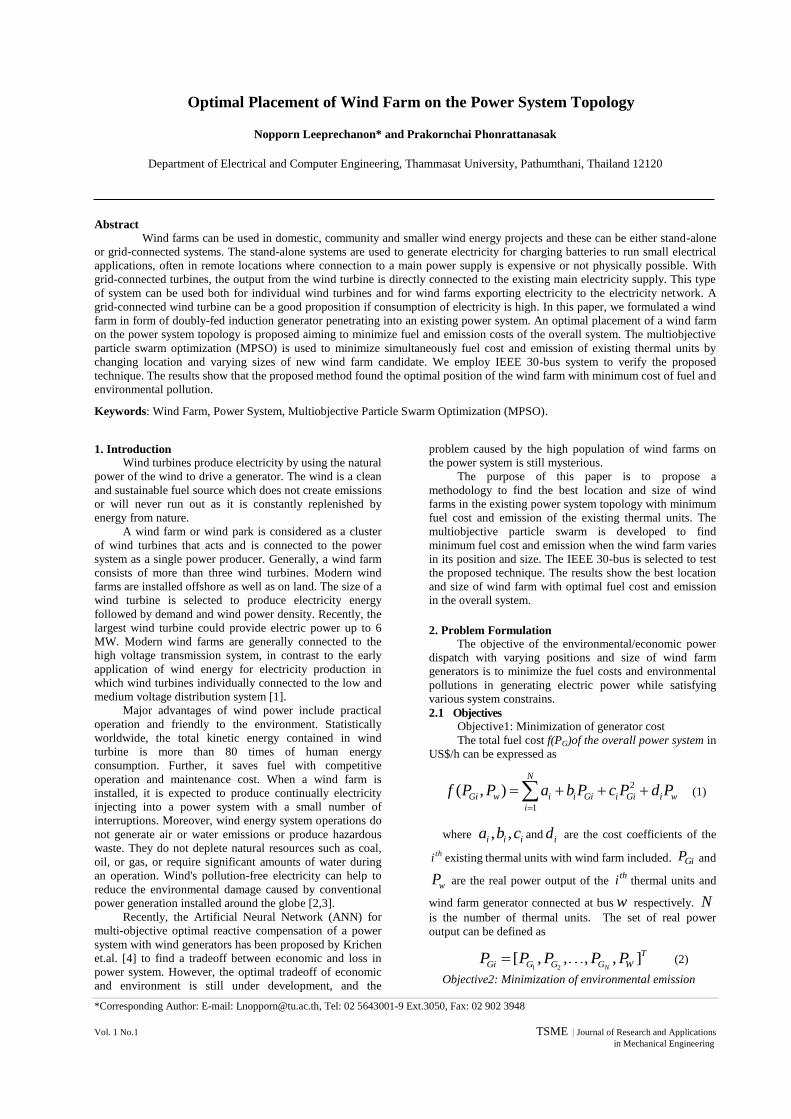
proportional to the wind speed. The example of a wind
farm is shown in Fig.1
Fig.1. A wind farm with many wind turbines connected to a
power system
In this paper, the cost and emission coefficients
of wind farms are zero. A large wind turbine is selected to
produce electric power up to 1.5 MW. The minimum
capacity of a wind farm is set as 4.5 MW or 3 wind turbines
and the maximum capacity of wind farm is set as 105 MW
or 70 wind turbines. These wind turbines run at speed of
wind as 12 m/s.
5. RESULTS AND DISCUSSION
Case 1: best fuel cost and emission of power system
without wind farm
Fuel cost and emission objective are optimized to find
the best solution by using MPSO Algorithm when the wind
farm is not penetrated into the power system network. Its
result is shown in Table 2.
Table 2. Best solution of the proposed approach without
wind farm
Unit (MW) Best solution
PG1 114.165
PG2 63.942
PG3 20.289
PG4 30.381
PG5 28.192
PG6 33.782
Total of thermal units (MW) 290.751
Fuel Cost($/h) 847.430
Emission(ton/hr) 0.245
Case 2: best fuel cost and emission of power system with
wind farm penetration
Table 3. Results of best solution of the proposed approach
with wind farm on IEEE 30-bus test system
Unit (MW) Best solution with
wind farm
PG1 48.454
PG2 34.443
PG3 30.439
PG4 29.079
PG5 16.122
PG6 28.612
Total of thermal units (MW) 187.149
Fuel Cost($/h) 541.52
Emission(ton/hr) 0.209
Wind farm
Location (Bus) 7
Size (MW) 99.73
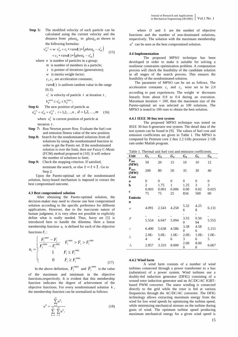
The wind farm is penetrated into the IEEE 30- bus
test system. Its result can be shown in Table 3 and Fig 2.
Table 3 shows the power generation and wind
farm position optimized by the MPSO technique. The result
in this case produces lower cost and emission than the
previous case. The wind farm which is penetrated into the
IEEE 30-bus test system can reduce fuel cost and emission
of pollution as 305.91 $/h and 0.036 ton/h respectively.
A wind farm is connected to the power system at bus 7
in Fig 2. The capacity of wind farm is 99.73 MW or
approximately 66 wind turbines. The result shows a high
penetration of wind farm on the test system.
Fig.2 Optimal position of wind farm on a power system
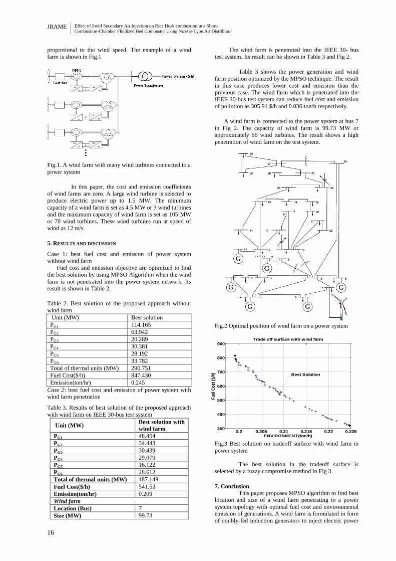
Fig.3 Best solution on tradeoff surface with wind farm in
power system
The best solution in the tradeoff surface is
selected by a fuzzy compromise method in Fig 3.
7. Conclusion
This paper proposes MPSO algorithm to find best
location and size of a wind farm penetrating to a power
system topology with optimal fuel cost and environmental
emission of generations. A wind farm is formulated in form
of doubly-fed induction generators to inject electric power
0.2 0.205 0.21 0.215 0.22 0.225300
400
500
600
700
800
900
ENVIRONMENT(ton/h)
Fu
el C
ost
($/
h)
Trade off surface with wind farm
Best Solution

Journal of Research and Applications
in Mechanical Engineering (JRAME) Vol.1 No. 1
17
into the power system. The simulation results demonstrate
that a wind farm with optimum size and location can reduce
fuel cost and emission pollutant of generators. In addition,
the results confirm that the MPSO algorithm has
effectiveness to search optimum position and size of wind
farm on a power system topology.
8. Reference [1] Chen, Z., Blaabjerg, F., 2009. Wind farm-A power source in future power systems. Renewable and Sustainable Energy
Reviews, Vol. 13, No. 6-7, pp.1288-1300.
[2] Lin, C.J., Yu, O.S., Chang, C.L., Liu, Y.H., Chuang, Y.F., Lin, Y.L., 2007. Challenges of wind farms connection to future
power systems in Taiwan. Renewable Energy, Vol. 34, No. 8. [3] Saidur, R., Islam, M.R., Rahim, N.A., Solangi, K.H., 2010.
A review on global wind energy policy. Renewable and
Sustainable Energy Reviews, Vol. 14, No. 7 pp. 1744-1762. [4] Krichen, L., Aribia, H.B., Abdallah, H.H., Ouali, A., 2008.
ANN for multi-objective optimal reactive compensation of a power
system with wind generators. Electric Power Systems Research, Vol. 78, No. 9, pp. 1511-1519.
[5] Abido, M.A., 2009. Multiobjective particle swarm optimization
for environmental/economic dispatch problem. Electric Power Systems Research, Vol. 79, No. 7, pp. 1105-1113.
[6] Sag, T., Cunkas, M., 2009. A tool for multiobjective
evolutionary algorithms. Advances in Engineering Software, Vol. 40, No. 9, pp. 902-912.
[7] Kennedy, J., Eberhart, R., 1995. Particle swarm optimization.
In: Proceeding of the 4th IEEE International Conference on Neural Networks, pp. 1942-1948.
[8] Abido, M.A., 2002. Optimal power flow using particle swarm
optimization. International Journal of Electrical Power & Energy Systems, Vol. 24, No. 7, pp. 563-571.
[9] Alsac, O., Stott, B., 1974. Optimal Load Flow with Steady-
State Security. Power Apparatus and Systems, IEEE Transactions on , Vol. PAS-93, No. 3, pp.745-751.
[10] Mendoza, F., Bernal-Agustin, J.L., Dominguez-Navarro, J.A.,
2006. NSGA and SPEA Applied to Multiobjective Design of Power Distribution Systems. Power Systems, IEEE Transactions
on, Vol. 21, No. 4, pp.1938-1945.

*Corresponding Author: E-mail: [email protected]
Vol. 1 No.1 TSME | Journal of Research and Applications in Mechanical Engineering
Passive vibration control of an automotive component using evolutionary optimisation
Nantiwat Pholdee1 and Sujin Bureerat*2
1,2Department of Mechanical Engineering, Faculty of Engineering, Khon Kaen University,
Khon Kaen, Thailand 40002
Abstract
In this paper, the use of multiobjective evolutionary optimisers for passive vibration suppression of an automotive
component is demonstrated. The component is used to connect a car engine to some point of a car body between the front seats.
Under such a circumstance, the structure is subject to several mechanical phenomena e.g. stress failure, fatigue, vibration
resonance, and vibration transmissibility. The optimisation problem is posed to find structural shape and size such that
maximising structural natural frequency and simultaneously minimising structural mass while constraints include stress failure
and displacement. The multiobjective optimiser employed is the multiobjective version of Population-Based Incremental
Learning (PBIL) with and without using a surrogate model. The optimum results obtained are illustrated and discussed. It is
found that the proposed design scheme is effective and efficient for an automotive component design.
Keywords: multiobjective evolutionary algorithm; shape optimisation; Pareto optimal front; automotive component; Vibration
suppression
1. Introduction
Due to highly increasing competitiveness in
automotive industry, many car manufacturers require to
develop new products to offer to customers. Therefore,
automotive components are always improved by means of
design optimisation [1-2].
Practical engineering design problems are usually
assigned to find the best solutions of design variables that
lead to optimised design objectives whilst fulfilling all the
predefined constraints. Often, the design problem has more
than one objective which is called multiobjective
optimisation. The most popular method used for the
multiobjective optimisation is Evolutionary Algorithms
(EAs) [3-6]. The method can explore a Pareto optimum
front within a single run and without requiring function
derivatives. However, a lack of search consistency and low
convergence rate are the inevitable drawbacks of the
multiobjective evolutionary algorithms (MOEAs) [5]. For
this reason, the hybridisation of a surrogate model method
and multiobjective optimisers has been invented and this
approach is found to be very powerful and effective [6].
This paper presents the multiobjective
evolutionary optimisation of an automotive component.
The component is used to connect a car engine to some
point of the body between the front seats. The structure is
subject to several mechanical phenomena such as stress
failure, fatigue, vibration resonance, and vibration
transmissibility. The design problem is posed to find
structural shape and size such that maximising structural
dynamic stiffness while, at the same run, minimising
structural mass. Design constraints include stress and
displacement. Three dimensional finite element analysis
(FEA) is employed to evaluate the objective and constrain
function values. The optimum solutions called Pareto
solutions are explored by using PBIL incorporating with a
Gaussian process surrogate model and a Latin Hypercube
Sampling technique. The proposed design approach is
found to be numerically powerful and effective.
2. Surrogate model method
The term‟ surrogate model‟ used in an optimisation
process is an approximate model which is used to
approximate the objective and constrain functions in
optimisation problems [7]. Such a design strategy is useful
when dealing with optimisation problems with expensive
function evaluation, limited function values available, and
problems that need to perform an experiment to evaluate
their function values. The hybrid of the surrogate model
with an optimiser can be achieved in several ways. One of
the commonly used strategies is that, during the main
optimisation process, some design solutions have been
evaluated. Those solutions and their corresponding
objective and constraint values are used to build a surrogate
model. This model is then used as an approximate function
evaluation. The optimisation with the surrogate model is
performed with significantly less running time when
compared with using the actual function evaluation. The
obtained optimum solution of this design phase is brought
to the main optimisation process where its actual function
value is determined. With a highly accurate surrogate
model, this design strategy is far superior to purely using an
evolutionary algorithm. The computational steps are
repeated until the termination conditions are fulfilled. The
commonly used surrogate models for optimisation are
Kriging model [8], radial basis interpolation [6],
polynomial interpolation [9] and neural network [10]. In
this paper, only the Kriging model is employed.
2.1. Kriging Model
A Kriging model (also known as a Gaussian
process model) used herein is the famous MATLAB
toolbox named Design and Analysis of Computer
Experiments (DACE) [8]. The estimation of function can
be thought of as the combination of global and local
approximation models i.e.

JRAME Passive vibration control of an automotive component using evolutionary optimisation
20
)()()( xxx Zfy (1)
where
)(xf is a global regression model, )(xZ is a
stochastic Gaussian process with zero mean and non-zero
covariance representing a localised deviation, and x is a
design variables vector. In this work, a linear function is
use for a global model, which can be expressed as:
fβ
T
n
1iii0 xββf (2)
where β = [β0, …, βn]T, f = f(x) = [1, x1, x2, …, xn]
T. The
covariance of Z(x) is expressed as:
)],([))(),(( 2 qpqp RZZCov xxRxx (3)
for p, q = 1, …, N where R is the correlation function
between any two of the N design points, and R is the
symmetric correlation matrix size NN with the unity
diagonal [8]. The correlation function used in this paper is
))()(exp(),( qpTqpqpR xxθxxxx
(4)
where i are the unknown correlation parameters to be
determined by means of the maximum likelihood method.
Having found and , the Kriging predictor can be
achieved as
) ()()( 1FβyRxrβxf TTy (5)
Where = [f(x1), f(x2), …, f(xn)]T and ( ) ( ) ( ) ( ) . For more details, see [8].
3. Multiobjective Population-Based Incremental
Learning (MOPBIL)
PBIL algorithm is an evolutionary optimiser based
upon binary searching space. The PBIL approach evolves its
population based upon the so-called probability vector, the
probability of having „1‟ elements on each column of a
binary population. The example of how the probability
vector works is shown in Fig.1 which implies that one
probability vector can produce a variety of binary
populations.
In the multiobjective optimisation, more probability
vectors should be used in order to obtain a more diverse
population; therefore, it is called a probability matrix.
Starting with an initial probability matrix that have all
elements as “0.5”, and an initial Pareto archive, the binary
population according to the initial probability matrix is then
created. The binary population is decoded and objective
values are evaluated. The best binary solutions, whether it is
based on minimisation or maximisation, is chosen to update
the probability vector newjiP , for the next iteration using the
relation
RjRoldji
newji LLPP b)1(,, (6)
where LR is called the learning rate, a value between 0 and
1, to be defined and bi is the mean value of the jth column of
the randomly selected non-dominated binary solutions. For
this study, LR is set as:
)1.0or 1.0(5.0 randLR (7)
where rand [0,1] is a uniform random number. Mutation
on the thi row of the probability matrix is allowed to take
place by a predefined probability and it can be expressed
as: ss
oldji
newji )mrandmPP 1or 0()1(,, (8)
where s
m is the amount of shift used in the mutation.
Fig.1 Probability vector and their corresponding
populations
The updating process is completed when all rows of
the probability matrix are changed. The probability matrix
is updated and the external Pareto archive is improved
iteratively until convergence is achieved.
In cases where the total number of the non-dominated
solutions is greater than the archive size, the archiving
operator called the normal line method [4] is activated to
remove some solutions from the archive. The archiving
technique is used to prevent excessive use of computer
memory during an optimisation process. The basic idea of
the normal line technique is used to remove some non-
dominated design solutions while maintaining population
diversity in the archive. For more details of multiobjective
PBIL, see [11].
4. Design Problem
This paper presents a multiobjective optimisation
design problem for an automotive part as shown in Fig. 2.
The component is used to connect the car engine with the
car body. Under the working conditions, this structure is
subject to several mechanical phenomena e.g. stress,
fatigues, vibration resonance, and dynamic force
transmissibility. Also, the structural displacement due to a
number of loading conditions should not exceed the
predefined limit.
Fig. 2 Automotive part
Fig. 3 a. Sizing variables
Part to be designed
population 1 population 2 population 3
0 0 1 1 0 1 1 0 0 1 0 1
1 1 0 0 1 1 0 0 1 0 0 1
0 0 1 1 1 0 1 0 0 0 0 1
1 1 0 0 0 0 0 1 0 1 0 0
Probability Vectors
[0.5,0.5,0.5,0.5] [0.5,0.5,0.5] [0.25,0.5,0,0.75]

Journal of Research and Applications
in Mechanical Engineering (JRAME) Vol.1 No. 1
21
Fig. 3 b. Shape variables
The multiobjective optimisation problem is posed to
find structural shape and size such that maximising
structural natural frequencies and minimising mass whereas
constraint include stress failure and displacement, which
can be expressed as
Min: )](),([ 21 xxf ff (9)
Subject to
allowablemax
0.005maxu
0.01x0.005
0.01x0.01
0.03z0
0.005z0.01
0.005z0.01
0.0028z0.0025
0.01z0.003
0.015t0.0025
0.01t0.0015
0.0115t0.0015
0.0115t0.0015
2
1
5
4
3
2
1
4
3
2
1
where x is a design variable vector (all variables are
displayed in Fig. 3). 1f is a function of mass. 2f is a
function of dynamic stiffness (or natural frequencies). x ,
1f and 2f can be express as :
T,x,x,z,z,z,z,z,t,t,tt }{ 21543214321x
and massf 1 (10)
and
54321
2
1
f . (11)
The other parameters are defined as follows:
maxσ = Maximum von Misses stress
allowableσ = Allowable stress
ti =Shape thickness
zi=Position of the key points in z-axis direction
xi= Position of key point in x-axis direction
i = mode ith natural frequency of a structure
Figs. 3a. & 3b. display all of the sizing and shape
design variables. The thicknesses (ti in Fig. 3 a.) are the
thickness of the sub-regions of the automotive component
as shown. The zi parameters determine the key points in
vertical direction as located in Fig. 3 b. These key points
are used to generated a spline curve so as to define the
shape of the part. The xi parameters define the horizontal
position of the key points on the component.
The structure is acted upon by three load cases
(bending, twisting and swaying loads) at the right-hand
cylinder part. The objective and constraint function values
are evaluated by using FEA. The evaluation process is
carried out in such a way that, with the given input design
variables as defined, the shape and dimensions of the
structure are created. The finite element analysis is then
performed. Finally the computational results can be
obtained. Function evaluation is somewhat time-
consuming, which means it is difficult to apply a common
evolutionary algorithm to solve the optimisation problem
(9). As a result, the surrogate-assisted evolutionary
algorithm is developed to deal with such a difficulty.
To tackle multiobjective optimisation as defined
in (9), the MOPBIL algorithm and the surrogate-assist
MOPBIL (MOPBIL-SM) are used to find Pareto optimal
solutions. MOPBIL-SM is a design strategy that exploits
the surrogate model to create an initial Pareto archive rather
than starting with a randomly generated population as with
the traditional multiobjective PBIL.
The computational steps for generating an initial
Pareto archive by using the surrogate model are as follows:
I. Sample a set of design variable vectors from
design experiment by using the LHS technique.
II. Evaluate design functions by FEA.
III. Constructing a surrogate model by using the
Kriging technique.
IV. Use MOPBIL find Pareto optimal set based on
the surrogate model.
V. Find the real function values of the Pareto
optimal front obtained from optimising the
approximate Kriging model (step IV).
VI. Use a non-dominated sorting technique to find
the initial Pareto archive
The LHS is used to sample 100 design solutions
for constructing a surrogate optimisation model.
Subsequently, with this initial Pareto archive, the common
MOPBIL is operated where the population size is 30, the
number of iterations is 10, and archive size is set as 30.
5. Results and Discussion
The progress of Pareto optimal solutions of the
optimisation design problem by using the hybridisation of a
surrogate model method and the MOPBIL is displayed in
Fig. 4. It can be seen that the Pareto front from iteration 1
to iteration 10 has slight improvement. This means that the
initial front generated by means of a surrogate-assisted
approach is very powerful.
Fig.4 Pareto front of the MOPBIL-SM
In order to verify the effectiveness of the hybrid
approach, the original MOPBIL without the use of a
surrogate approach is performed with the same population
and archive sizes while the total generation number is set to
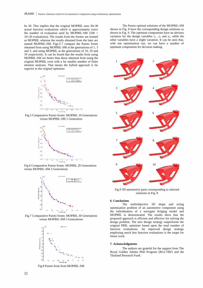
JRAME Passive vibration control of an automotive component using evolutionary optimisation
22
be 30. This implies that the original MOPBIL uses 3030
actual function evaluations which is approximately twice
the number of evaluation used by MOPBIL-SM (100 +
1030 evaluations). The results from the former are termed
as MOPBIL whereas the results obtained from the later are
named MOPBIL-SM. Figs.5-7 compare the Pareto fronts
obtained from using MOPBIL-SM at the generations of 1, 3
and 5, and using MOPBIL at the generations of 10, 20 and
30 respectively. It can be found that the results from using
MOPBIL-SM are better than those obtained from using the
original MOPBIL even with a far smaller number of finite
element analyses. That means the hybrid approach is far
superior to the original optimiser.
Fig.5 Comparative Pareto fronts: MOPBIL 10 Generations
versus MOPBIL-SM 1 Generation
Fig.6 Comparative Pareto fronts: MOPBIL 20 Generations
versus MOPBIL-SM 3 Generations
Fig.7 Comparative Pareto fronts: MOPBIL 30 Generations
versus MOPBIL-SM 5 Generations
Fig.8 Pareto front from MOPBIL-SM
The Pareto optimal solutions of the MOPBIL-SM
shown in Fig. 8 have the corresponding design solutions as
shown in Fig. 9. The optimum components have an obvious
variation for the design variables t2 , z3 and z5, while the
other variables have a slight variation. It can be seen that,
with one optimisation run, we can have a number of
optimum components for decision making.
Fig.9 3D automotive parts corresponding to selected
solutions in Fig. 8
6. Conclusions
The multiobjective 3D shape and sizing
optimisation problem of an automotive component using
the hybridisation of a surrogate Kriging model and
MOPBIL is demonstrated. The results show that the
proposed approach is efficient and effective for solving the
design problem. The new design strategy outperforms the
original PBIL optimiser based upon the total number of
function evaluations. An improved design strategy
employing much less function evaluations is the target for
future work.
7. Acknowledgments
The authors are grateful for the support from The
Royal Golden Jubilee PhD Program (RGJ-TRF) and the
Thailand Research Fund.
1 2
3 4
5 6
7 8
9 10

Journal of Research and Applications
in Mechanical Engineering (JRAME) Vol.1 No. 1
23
8. References
[1] Kaya, N., Karen, I., Öztürk, F., 2010. Re-design of a failed
clutch fork using topology and shape optimisation by the response
surface method. Materials and Design, Vol. 31, pp. 3008-3014. [2] Torstenfelt, B., Klarbring, A., 2007. Conceptual optimal design
of modular car product families using simultaneous size. shape and
topology optimization, Finite Elements in Analysis and Design, Vol. 43, pp. 1050-1061.
[3] Bureerat, S., Sriworamas, K., 2007. Population-Based
Incremental Learning for Multiobjective Optimisation, Advance in Soft Computing, Vol. 9, pp. 223-231.
[4] Kanyakam, S., Bureerat, S., 2007. Passive Vibration
Suppression of a Walking Heat and Mass Tractor Handlebar Structure Using Multiobjective PBIL. In: Proceedings of the 2007
IEEE Congress on Evolutionary Computation, Singapore.
[5] Kanyakam, S., Srisomporn, S., Bureerat, S., 2009. Optimal Geometrical Design of Multiple Heights Pin-Fin Heat Sink Using
MOPBIL. In: Proceedings of the 23rd Conference of the
Mechanical Engineering Network of Thailand, Chiang Mai, Thailand.
[6] S., Srisomporn, S., Bureerat, 2008. Geometrical Design of
Plate-Fin Heat Sinks Using Hybridization of MOEA and RSM, IEEE TRANSACTIONS ON COMPONENTS AND
PACKAGING TECHNOLOGIES, Vol. 31, pp. 351-360.
[7] Liao, X., Li, Q., Yang, X., Zhang, W., Li, W., (2008). Multiobjective optimization for crash safety design of vehicles
using stepwise regression model. Struct Multidisc Optim, Vol. 35,
pp. 561–569. [8] Lophaven, SN., Neilson, HB., Sondergaard, J., DACE a
MATLAB Kriging Toolbox. Technical report IMM-TR-2002-12,
Technical University of Denmark. [9] Zhou, Z., Ong, YS., Lim, MH., 2007. Memetic algorithm using
multi-surrogates for computationally expensive optimization
problems. Soft Computing, Vol. 11, pp. 957-971. [10] Farina, M., Amato, P., 2005. Linked interpolation-
optimization strategies for multicriteria optimization problems.
Soft computing, Vol. 9, pp. 54-65. [11] Bureerat, S., Srisomporn, S., 2010. Optimum plate-fin heat
sinks by using a multi-objective evolutionary algorithm.
Engineering Optimization, Vol. 42, pp. 305-343.

*Corresponding Author: E-mail: [email protected], Tel: 02 218 6610, Fax: 02 252 2889
Vol. 1 No.1 TSME | Journal of Research and Applications in Mechanical Engineering
The Effect of Interference Fit on Vibration Transmission from Stator Coil to Base of
a Spindle Motor in a Hard Disk Drive
Nopdanai Ajavakom1,* and Apirat Sillapapinij1
1 Department of Mechanical Engineering, Faculty of Engineering, Chulalongkorn University, Bangkok, Thailand 10330
Abstract
The hard disk drive spindle motor is the primary source of vibrations that cause acoustic noise in the hard disk drive
(HDD). The electromagnetic forces on the stator coil and the rotor, which are inherent to the operation of motors, are responsible
for the deformation causing vibration of the motor’s interior structure. This vibration is transmitted to the motor exterior
especially the motor base through the fit between the stator coil and the motor base. This article proposes an approach to reduce
the acoustic noise of the HDD is hence by reducing the transmitted vibrational energy from the stator coil to the base by
optimizing the interference fit between these two components. The effect of the fit on the transmitted vibrational energy through
both the vibrational energy analysis through a friction model featuring micro-slip and the experimental investigations is studied.
The vibrational energy analysis is applied on a hollow cylinder installed on a shaft as a simplified model of the stator coil and the
base. The analysis shows that the transmitted torsional vibrational energy is proportional to the pressure due to the interference
fit. Hence, it suggests that the reduction of the vibration transmission from the stator coil to the base can be done by decreasing
the interference fit. In addition, the experimental investigations performed on three simple models of stator and base with
different interference fits and also two groups of spindle motor samples with different fits agree well with the analysis.
Keywords: Interference fit, spindle motor, vibration transmission, statistical energy analysis
1. Introduction
A hard disk drive (HDD) is an important component
in a personal computer to store the data. In need of higher
performance HDDs including higher capacity, faster data
read/write time, quieter operation while maintaining or
even reducing the HDD physical size, the spindle motors
are required to spin faster and smoother. Thus, the vibration
transmitting from the interior to the exterior of the spindle
motor, which may finally cause the data read/write errors
and the emission the acoustic noise, has to be looked into.
The primary source of vibration inside the motor is the
electromagnetic (EM) sources, not the mechanical
unbalance of the moving parts [1,2]. The EM sources are
originated from the physical and the electromagnetic
designs of the permanent magnet ring and the stator teeth of
the motor as well as the characteristics of the input power
from the motor inverter. The designs contribute the
unbalance radial, tangential, and axial forces on the
permanent magnet ring and the stator teeth deforming the
interior structure of the motor. The deformations of the
stator teeth, especially from varying tangential forces
(torque ripple), are transmitted to the base bracket via the
cylindrical-shell sleeve causing transverse vibration of the
base plate [3]. Moreover, the deformations of the ring
propagate into rotor hub as transverse and radial vibrations
[3]. The vibrations of the motor exterior are responsible for
the acoustic noise emitted from the motor. The approaches
to decrease the vibrations and the acoustic noise from the
motor include the elimination of EM sources, modification
of the motor physical design to minimize the sound
radiation, and reduction of the vibration transmission from
the motor interior to the exterior, for example, by
optimizing the interference fit between the stator coil and
the base bracket. See Fig.1.
This article focuses on the effect of interference
fit between the stator coil and the base of the spindle motor
on the torsional vibrational energy transmission from the
stator coil to the base plate aiming to reduce the transmitted
energy capable of the motor’s exterior vibrations and the
emitted acoustic noise. The article presents both vibration
energy transmission analysis and two experimental
investigations.
Fig. 1 Cross-section view of a spindle motor showing the
fit between the stator coil and the base bracket
2. Vibrational Energy Transmission Analysis
The analysis of vibrational energy transmission
between the stator coil and the base of the motor involves a
friction model and vibration transmission mechanism of the
two surfaces in contact with the clamping pressure.
Jintanawan et al. [4] study a simple dynamic model of the
stator coil and the base of a spindle motor featuring the
two-degree of freedom lumped mass model attached to a
fixed foundation via a torsional spring. The Dahl’s model is
used to analyze the relative angular displacement between
the two components due to the applied impulsive torque at
the stator coil. The study shows that the more the
interference fit is, the more the vibrational energy is
transmitted to the base and vice versa.
Nevertheless, for the continuous and more
complex system, such as the spindle motor, the analysis
that considers the internal forces on the surfaces, the micro-
slip, the pre-sliding behavior, and the force’s loading-
unloading-reloading stages is more suitable. Such an
analysis by Metherell and Diller [5] is modified to work on
a stator-base model of a spindle motor. It will be shown
from the hysteresis diagram of the torque versus the

JRAME The Effect of Interference Fit on Vibration Transmission from Stator Coil to Base of a Spindle Motor in a Hard Disk Drive
26
relative angular displacement that the vibrational energy
loss is lower (the energy transmission is higher) as the
interference fit is more.
Fig. 2 Simple model of stator and base bracket
Fig. 3 Dynamic model of stator and base
Consider the simplified stator-base model shown
in Fig. 2 where the stator is a ring press-fit into the base
bracket via a sleeve. To simplify the analysis, the sleeve is
assumed to be a solid shaft of radius R and the ring is
assumed to be a hollow cylinder of length l shown in the
dynamic model in Fig. 3. Torques are applied to the left
side of the cylinder and the right side of the shaft. They are
opposite with the equal magnitude of M , where
10 , preventing any angular displacement of the
whole assembly. The micro-slip is taken into account and
the concept of Coulomb friction is used, the torsional
friction per unit length of the cylinder on the contact
surfaces is then 22 PRm , (1)
where m is the torsional friction per unit length (N-m/m),
is coefficient of friction,
P is the pressure between the cylinder and the shaft
due to the fit (Pa),
R is the radius of the shaft (m). In our case,
according to Eq. (1), the torsional friction per unit length is,
in general, constant over the length of the cylinder due to
the constant interference fit pressure, coefficient of friction
and radius of the shaft. In one cycle of the varying applied
torque, the torque is exerted to the model in three non-stop
consecutive stages: loading, unloading, and reloading.
In the loading stage, the applied torque on the
cylinder increases from 0 to M , that is M , where
increases from 0 to 1. At the same time, the resisting torque
at the shaft increases to balance out the applied torque
creating friction on the contact surfaces. The diagrams of
the torsional friction per unit length, the internal torsion on
the cylinder surface, and the internal torsion on the shaft
surface are shown in Fig. 4. The torsional friction per unit
length is m with the exception of being zero in the
middleregion of the length of the cylinder where there is no
slipping. The slipping and the torsional friction occur at the
left and right edge of the contact surfaces with length on
each side equals 1a
( 2/0 1 la ), where 1a depends on the magnitude of the
applied torque. The internal torsion on the cylinder surface
is M at the left edge and it decreases with the slope m
as it goes to the right. Likewise, the internal torsion at the
shaft surface is M at the right edge and decrease with the
slope m as it goes to the left. In addition, the summation
of internal torsions at the cylinder and the shaft surfaces
must be equal to M along the length of the cylinder.
In the unloading stage, being reverse to the
loading stage, the applied torque M on the cylinder now
decreases from M to rM as decreases from 1 to r ,
where r is constant and 10 r . Since the applied torque
decreases, the torsional friction per unit length is now m
making the internal torsion on the cylinder surface
increases with the slope m as it goes to the left. The
phenomenon is called “counter slip.” The counter slip
occurs for the length of 2a . The further inside region of the
cylinder and the shaft still experiences the torsional friction
m remaining from the loading stage. The diagrams of the
torsional friction per unit length, the internal torsion on the
cylinder surface, and the internal torsion on the shaft
surface for the unloading stage are shown in Fig. 5.
In the reloading stage, quite similar to the loading
stage and reverse to the unloading stage, the applied torque
M on the cylinder increases back from rM to M as
increases from r to 1, where 10 r . The torsional
friction per unit length currently returns to m at the left
and right sides of the cylinder. The diagrams of the
torsional friction per unit length, the internal torsion on the
cylinder surface, and the internal torsion on the shaft
surface of the reloading stage are shown in Fig. 6.
Fig. 4 Loading stage diagram

Journal of Research and Applications
in Mechanical Engineering (JRAME) Vol.1 No. 1
27
Fig. 5 Unloading stage diagram
Fig. 6 Reloading stage diagram
The relative angular displacement of each stage
can be determined from the torsional friction per unit
length, the internal torsions on the surfaces, the shaft’s and
the cylinder’s material properties, and other previously
introduced constants:
kImG
Mkk
IG
Mlk
ssss
12
331 222
1
, 10 (2)
kImG
kkM
IG
Mlk
ssss
14
331 21 222
2
,
10 r (3)
ss IG
Mlk 3
kImG
kkrrM
ss
14
331 221 222 ,
10 r (4)
ccss
ss
IGIG
IGk
(5)
where 1 , 2 , 3 are the relative angular displacements
for the loading, unloading, and reloading stages,
respectively, cc IG and ss IG are the torsional stiffness of
the cylinder and the shaft, respectively, and k is the
combined torsional stiffness of the cylinder and the shaft.
The angular displacements can be plotted against to
form a hysteresis loop depicted in Fig. 7.
The transmission energy loss due to the friction
of the fit can be obtained from the area enclosed by the
relative angular displacements under the three stages over
one cycle,
kImG
kkM
ss
a
13
3312 23
(6)
where is the energy loss due to friction (J) and
rMMa 12
1 , 10 r (7)
According to Eqs. (6) and (7), the transmission energy loss
depends on the cube of the applied torque and inversely
depends on the torsional friction per unit length given that
the other parameters are constant. Focusing on the effect of
the interference fit, the equations indicate that the energy
loss is less when the torsional friction is larger because of
the more pressure from the tighter interference fit, Eq. (1).
That is, the transmitted vibrational energy from the stator to
the base would be more if the interference fit increases.
This statement can also be testified by the experimental
investigations in the next section.
Fig. 7 Hysteresis loop of the dynamic model
3. Experimental Investigations
The experimental investigations are performed to
testify the analytical results in the previous section. Sets of
simple models of stator coil and base and 3.5-inch HDD
spindle motor samples with various fits are made and tested
in Sections 3.1 and 3.2, respectively. The tests were done
on the simple models first and on the motor samples later.
3.1 Simple models of stator coil and base
Three sets of 1.5x-size model of stator coil and
base (see Fig. 8) with three interference fits, 0.0083 mm
(minimum fit), 0.0169 mm (medium fit) and 0.0304 mm
(maximum fit), are tested for the energy transmitted from
the stator to the base. The transmission of energy between
two systems, stator (system 1) and base (system 2), is
analyzed by using Statistical Energy Analysis (SEA) [6, 7].
The power flow diagram is shown in Fig. 9. The input
power 1P from the impact force exerted by the impact
hammer at the stator model will go to raise the stator model
internal energy 1W , which is related to the power loss to

JRAME The Effect of Interference Fit on Vibration Transmission from Stator Coil to Base of a Spindle Motor in a Hard Disk Drive
28
the environment 11P and the power transmitted to the base
model 12P . The power loss 11P is
11 11 WP , (8)
where is the frequency and 1 is the intrinsic loss
factor. The transmitted power 12P is
112 12 WP , (9)
where 12 is the coupling loss factor from stator to base.
The power equation of the stator model is then
2112111 PPPP , (10)
where 21P is the power received from the base. This power
also depends on the base model internal energy 2W and
221 21 WP , (11)
where 21 is the coupling loss factor from base to stator.
Applying the same concept to base model where there is no
direct input power from the impact hammer, the power
equation of the base model is thus
1221220 PPP , (12)
where 22P is the power loss to the environment and
22 22 WP , (13)
where 2 is the intrinsic loss factor of system 2.
The approach to determine the transmitted power
12P starts with tests to find the intrinsic loss factor of either
of the two systems. The test is performed on either system
separately, i.e. the stator model has not yet fit into the base
model, where 12P and 21P are non-existent and
11 111 WPP . (14)
The stator is then press-fit into the base. In order to
simplify the testing for the power transmission, the base is
damped out by attaching it to the large mass for minimizing
2W and thus 21P is near zero according to Eq. (11). With
the known input power 1P , the intrinsic loss factors
1 , 2 , the coupling loss factor 12 as well as the
transmitted power 12P can be calculated. With the roughly
equal input power 1P of approximately 41011.1 W, the
transmitted power 12P over the 20-kHz span for all three
sets with three different interference fits is shown in Fig. 10
and summarized in Table 1 with three equal ranges of
frequencies. It can be observed that by roughly looking at
the graph in Fig. 10 the system with the maximum
interference fit has the largest transmitted power among the
three systems at the frequency above 12 kHz. At the
frequency below 12 kHz, the lines, however, are not
smooth, which is suspected to be from some human
uncertainties in the experiment, e.g. from the uneven
impact force from the hammer. The numerical results for
each set in the frequency ranges listed in Table 1 also
indicate the similar trend. For the medium and high
frequency ranges, the maximum fit set has more
transmitted power than the other two sets. The medium fit
set has more transmitted power than the minimum fit set. In
short, generally speaking, the system with less fit possesses
less transmitted power. This is consistent with the
analytical results in Section 2.
Fig. 8 Assembled simple stator-base model
Fig. 9 Power transmission diagram of two systems
Fig. 10 Transmitted power from stator to base for three
interference fits
Table 1 Power transmitted to the base with different
interference fits (simple models)
Frequency
range/Model
fit
Transmitted power (W)
Min
(8.3 µm)
Med
(16.9 µm)
Max
(30.4 µm)
Low
(0-6.6 kHz)
1.45 1.69 1.12
Medium
(6.7-13.3
kHz)
1.40 1.34 2.44
High
(13.4-20 kHz)
2.05 2.09 3.26
Overall
(0-20 kHz)
4.90 5.12 6.82
Stator W1
P11
Base W2
P22
P12
P21
P1

Journal of Research and Applications
in Mechanical Engineering (JRAME) Vol.1 No. 1
29
3.2 3.5-inch hard disk drive spindle motors
Two groups of 3.5-inch HDD spindle motors,
3-phase permanent magnet synchronous motors (PMSMs),
with different interference fits; Group A with 0.016-and
0.018-mm fits (low fit) and Group B with 0.034-mm fit
(high fit), are tested to investigate the effects of stator-base
interference fit on the transmitted energy. The varying
frequency sinusoidal current is fed into only one phase
winding of the spindle motor to excite the stator coil and
the rotor structures without spinning the rotor. Particularly,
the induced vibration of the stator coil is transmitted to the
base plate where the transverse vibrations of 10 various
points are measured for calculating the vibrational energy
of the base. The transmitted vibrational energy is
determined from the spatial average square velocity from
the measure points and shown in joules per kg of mass per
ampere of the current input in Fig. 11 over a 20-kHz span.
Fig. 11 Vibrational energy of spindle motors with different
interference fits
The transmitted vibrational energies are also listed in Table
2 for three equal ranges of frequencies. The results indicate
that the vibrational energy over the low, the medium, the
high, and the overall frequency ranges of the motors with
less fit (Group A) is much lower than that of the motors
with more fit (Group B) especially at the low frequency
range. The motors with less interference fit between the
stator and the base has less transmitted vibrational energy
from the stator to the base than those with more
interference fit. These experimental results are consistent
with those from Section 3.1 and the analytical ones in
Section 2.
Table 2 Vibrational energy transmitted to the base with
different interference fits (HDD spindle motors)
Frequency
range/Motor group
Vibrational energy (µJ/kg/A)
A (16-18 µm) B (34 µm)
Low
(0-6.6 kHz)
1.164 6.067
Medium
(6.7-13.3 kHz)
4.063 7.263
High
(13.4-20 kHz)
0.938 1.004
Overall
(0-20 kHz)
6.164 14.33
4. Conclusion
The effect of interference fit on vibration
transmission from stator coil to base of a spindle motor in a
hard disk drive has been studied both analytically and
experimentally. The analysis of transmission energy loss
reveals that the energy loss inversely depends on the
pressure from the interference fit. Less energy loss and thus
more transmitted energy from the stator to the base are the
results of the more interference fit. The experimental
investigations on both assembled models of the stator and
the base and the spindle motor samples with various fits are
carried out and their results agree well with the analysis.
Hence, reducing the interference fit at the stator-base
assembly in the spindle motor is a promising approach to
reduce the transmitted vibrational energy to the base
bracket, and the acoustic noises emitting from the motor
should be lower.
5. References [1] Ajavakom, A., Jintanawan, T., Singhatanagid, P., Sripakagorn, P., 2007. On investigation of vibro-acoustics of FDB spindle
motors for hard disk drives, Microsystem Technologies, Vol. 13, No. 8-10, pp. 1281-1287.
[2] Lin, S., Jiang, Q., Mamun, A.A., Bi, C., 2003. Effects of drive
modes on the acoustic noise of fluid dynamic bearing spindle motors. IEEE Transactions on Magnetics, Vol. 39, pp. 3277-3279.
[3] Jintanawan, T., Sillapapinij, A., Ajavakom, N., 2009. Effects of
tolerance design on suppression of electromagnetic-induced acoustic noises and vibration transmission in hard disk drive
spindle motors. IEEE Transactions on Magnetics, Vol. 45, No. 11,
pp. 5129-5134. [4] Jintanawan, T., Chungphaisan, K., Liwcharoenchai, K.,
Junkaew, P., Singhatanagid, P., 2007. Role of stator-base
interference fit on vibration transmission and acoustic noise in FDB spindle motors for HDD. In: Proceedings of the Information
Storage Processing System Conference.
[5] Metherell, A.F., Diller, S.V., 1968. Instantaneous energy dissipation rate in a lap joint. Journal of Applied Mechanics, Vol.
35, pp. 123-128.
[6] Lyon, R.H., 1975. Statistical Energy Analysis of Dynamical Systems: Theory and Applications. The MIT Press Cambridge,
Massachusetts and London, England.
[7] Sarradj, E., 2004. Energy – based Vibroacoustics: SEA and Beyond. Gesellschaft für Akustikforschung Dresden mbH,
D-01099 Dresden, Germany.
Spatial avera
ged m
ean s
quare
velo
city

Vol. 1 No.1 TSME | Journal of Research and Applications in Mechanical Engineering
Transient Thermal Elastohydrodynamic of Rough Surfaces under Line Contact with Non-
Newtonian Solid-Liquid Lubricants
Chatchai Aiumpronsin1 and Mongkol Mongkolwongrojn 2
1 Mechatronics and Robotics Engineering Department, Faculty of Engineering, South-East Asia University, Bangkok, 10160. 2 Mechanical Engineering Department, Faculty of Engineering, King Mongkut’s Institute of Technology Ladkrabang,
Bangkok, 10520
Abstract
The thermal compressible elastohydrodynamic lubrication of rough surfaces under line contact with non-Newtonian solid-
liquid lubricants was investigated in transient operating conditions. Properties of non-Newtonian solid-liquid fluids have been
obtained experimentally using solid particles namely, Molybdenum disulfide. The newly derived time-dependent modified
Reynolds equation and the adiabatic energy equation have been formulated using a non-Newtonian power law viscosity model.
The simultaneous systems consisting of the modified Reynolds equation, elasticity equation and energy equation with initial
conditions were solved numerically using the multigrid multilevel method with a full approximation technique. The dynamic
characteristics of the two infinitely long cylindrical rough surfaces in line contact under thermoelastohydrodynamic lubrication
were presented with varying dimensionless time and with varying particle concentration for the pressure, temperature and oil film
thickness profiles. The results of rough surfaces thermoelastohydrohynamic lubrication with non-Newtonian solid-liquid
lubricants are compared with the case of smooth surfaces.
Keywords: Thermal elastohydrodynamic lubrication, Non-Newtonian solid liquid lubricants, Power law model, Modified
Reynolds equation.
1. Introduction
When lubricated contacts in machine element
applications are operated in severe conditions, the nominal
film thickness in the contacts can be decreased to a level where
surface roughness becomes significant. The lubricant film on
the solid surfaces of the machine components become very
thin. Therefore, the lubricant containing solid particles has
greatly improved the lubrication characteristics in order to
protect the contact surfaces. Many numerical solutions of
elastohydrodynamic lubrication (EHL) for smooth surfaces
and for rough surfaces problems were solved in the area
ranging from transient elastohydrodynamic to thermal
elastohydrodynamic using Newton-Raphson method and
multigrid multilevel with full approximate scheme techniques
[1-2]. In 1990, Khonsari, et al [3] showed that solid lubricant
additives have significant effects in raising the film thickness,
load capacity and friction coefficient in the full EHL regime.
Mongkolwongrojn [4] investigated the transient thermoelasto-
hydrodynamic lubrication with non-Newtonian liquid-solid
lubricants in line contact with smooth surfaces under a sudden
load change. The solid particles were found to have a
significant effect on the TEHL characteristics. In 2010,
Mongkolwongrojn [5] showed that the journal bearing with
transverse surface roughness pattern in the bearing liner
exhibit better stability.
In this research work, the integrated effect of moving
surface roughness and sudden loading on pressure profile, film
thickness profile and temperature profile is investigated
numerically in a TEHL line contact with non-Newtonian
liquid-solid lubricant using a power law model. Finite
difference multi-grid multi-level with full approximation
scheme techniques and Newton’s method were implemented to
examine the transient thermal elastohydrodynamic lubrication
with non-Newtonian liquid-solid lubricants under the action of
a sudden load change.
2. Governing Equations
2.1 Constitutive Equation
The governing modified Reynolds, elasticity, energy and
load equilibrium equations were analyzed to obtain transient
thermoelastohydrodynamic lubrication characteristics of two
rough surfaces in line contact under a sudden load change. The
relationship between shear stress and shear rate of the non-
Newtonian lubricant in this work can be approximated using a
power-law model as
*
xy u y (1)
where the equivalent viscosity is
1
2* 2
0
n
m u y
(2)
2.2 Modified Reynolds Equation
In this study, the flow can be approximated as a single-
phase flow. Integrating the momentum and continuity
equations, the time dependent modified Reynolds equation
with non-Newtonian lubricant for infinitely long cylindrical
roller can be obtained as.
3 0 0
2
2 1 1
11 2
2
e e
e e e
P SH K H K H K H
X X X X t
(3)
where 2 2
0
3 216H
u R UK
b P W
1
0*
,
1dY
Y j
je

JRAME Transient Thermal Elastohydrodynamic of Rough Surfaces under Line Contact with Non-Newtonian Solid-Liquid Lubricants
32
The boundary conditions are
0 ; PXX inlet and ;exitXX 0dX
dPP (4)
The apparent viscosity in the power-law model needs to be
included as a correction factor in the viscosity-temperature-
pressure relationship; the correction factor needs to be
modified for solid particles in the lubricant can be written as
1
11 ** 0 0
0 0
9 *
0 0
1 2.58 1
exp ln 9.67 1 1 5.1 10 1
nn
p
z
H
m u u
RWH Y
x P P T T
(5)
The dimensionless density of the liquid–solid lubricant varying
with pressure, temperature and mass concentration of particles
can be written as
p
H
H TTPPx
PPx
0
*09
9
11
11107.11
106.01
(6)
2.3 Elasticity Equation
The film thickness for an infinitely long line contact,
including the deformation of the surfaces and harmonic
roughness, is given as
tubX
lb
RAdXP
XHH
exit
inlet
X
X
12
2
0
2sinln
1
2
(7)
2.4 Energy Equation
The time-dependent energy equation in dimensionless
form was formulated including the heat generated due to
friction between the particles and surfaces. Therefore, the
energy can be expressed as
2 * 2 * *
*
12 *
2* * * 2 2
*
2 3 4*
exit
inlet
T
p
p
T T T X
p p p
X
T H T TK u
Y k t X
Wu T H P P HK K u K
k Y k t X kHdX
(8)
where
20
30
1Rk
bCuK
p
T
00
20
2Tk
uKT
20
3
3Rk
PbuK H
T
00
'
4Tk
bESufK
p
T
The boundary conditions of the energy equation are
i
in
X
X i
iii
i
ip
p
i
XX
dXTTT
H
k
SubkC
RkT
'
'*,1
*,2
*,
311,1
0*,1 426
21
1
(9)
i
in
X
X i
iii
i
ip
p
i
XX
dXTTT
H
k
SubkC
RkT
'
'*,1
**,2
,
322,2
0*,2 264
21
1
(10)
1)0(* XT (11)
The thermal model expressed by equation (8) to equation (10)
are equivalent to those models.
2.5 Load Carrying Capacity
Spherical shaped MoS2 particles are assumed to be
uniformly distributed in the contact region and the particles
undergo plastic deformation under the action of normal load.
For a particle that deforms plastically when the mean
contact pressure reaches the hardness of particle, dH , the
load carried by a plastically deformed particle can be
written as
2
3 3
,
9
16
p
p i d p i
ps
dw H p x A
E
(12)
where iA is the contact area of an individual particle
due to plastic deformation and ,p iw is the load supporting by
an individual particle. Therefore, the load carrying capacity
for all particles is
,
Z XN N
p p i
i i
w w (13)
The total load carrying capacity of the mixture consists of two
parts: one component results from plastic deformation of the
particles, pw , and the other component is due to
hydrodynamic action, fw . The dimensionless load balance
equation can be written as
1 02
exit
inlet
X
P
X
WPdX
W
(14)
During each time interval, the Reynolds, elasticity and
energy equations are calculated using the boundary conditions
and the initial conditions in Eq. (4), (9), (10) and (11) to
obtain pressure and temperature distributions. The relative
accuracy in pressure, mean temperature and hydrodynamic
load are less than or equal to 0.0001. The input parameters
used in the analysis are shown in Tables 1 and 2. The
properties of the lubricant as shown in Table 1 were obtained
experimentally. The Newtonian rheological model is used for
pure SAE90 oil with the power law index of n = 1. The
property values of MoS2 particles is shown in Table 2
Table 1 Physical properties of the SAE 90 oil and roller
material
Equivalent radius, m
Inlet temperature of lubricant, K
Viscosity of liquid, Pa.s
Inlet density of liquid, kg/m3
Viscosity-Pressure index
Viscosity-Temperature coefficient, K-1
Coefficient of thermal expansivity, K-1
Thermal conductivity of liquid , W/(m∙K)
Specific heat of liquid, J/(kg∙K)
Equivalent modulus of elasticity of
rolling/sliding, GPa
Poisson ratio of rolling/sliding
Wave length of roughness, (µm)
0.05
313
0.195
892.8
0.5685
0.05763
0.00074
0.126
1870
220
0.3
2.5

Journal of Research and Applications
in Mechanical Engineering (JRAME) Vol.1 No. 1
33
Table 2 Physical properties of solid lubricants, MoS2.
Density, kg/m3
Brinell hardness, Pa
Modulus of elasticity, GPa
Poisson ratio
Friction coefficient
4800
3.136 109
34
0.13
0.1
3. Results and Discussion
The static and dynamic characteristics of TEHL line
contact with non-Newtonian liquid-solid lubricants were
determined under the sudden dimensionless load change from
3.0x10⁻⁵ to 1x10⁻⁴ and dimensionless speed parameter U =
1x10-11.
The effects of heavy load change were investigated for a
surface with sinusoidal roughness of 0.05 μm amplitude using
SAE 90 oil mixed with 20% MoS2, 2 μm diameter, a load
increase from 3.0x10⁻⁵ to 1x10⁻⁴ at dimensionless speed
parameter U = 1x10-11 and slide/roll ratio S = 0.1. The
wavelength of the sinusoidal surface roughness profile in
transverse direction is kept fixed. The roughness induces
sharp pressure ripples over the ridges and valleys of the
roughness as shown in Fig.1. High fluctuating pressure
amplitude near the leading edge contrasts with the
fluctuating pressure amplitude near the trailing edge in
the contact region. At x = 0, the pressure fluctuations vary
from 0.36 GPa to 0.62 GPa under dimensionless load W =
3.0x10⁻⁵ at time t = 0 ms. After an application of the
sudden heavy load from 3.0x10⁻⁵ to 1x10⁻⁴, the fluctuating
pressure increases and varies from 0.65 GPa to 1.75 GPa
at time t = 6 ms. At the trailing edge, the pressure spike is
very large, approximately equal to 2.7 GPa at time t = 6 ms,
due to the significant effect on viscosity for a liquid-solid
lubricant with rough surfaces.
The transient oil film thickness under sudden load
change for sinusoidal surface roughness profile is shown in
Fig. 2. After application of a step load change, the central film
thickness at x = 0 mm increases form 1.40 μm at time t = 0.0
ms to 1.62 μm at time t = 1 ms but the minimum film thickness
decreases from 1.11 μm at t = 0.0 ms to 0.99 μm. at t = 1.0 ms.
Then the central film thickness at x = 0 mm decreases to 1.19
μm and the minimum film thickness decreases to 0.54 μm at
time t = 6 ms. the film thickness increase at x = 0 mm in the
early transient state is due to the interaction of pressure,
temperature and viscosity. Fig. 3 shows the fluctuating mean
temperature profile. The mean temperature at x = 0 mm varies
from 40.6C to 45.2C at time t = 0 ms. The temperature then
becomes very high after the step load increase and the mean
temperature varies from 88.4C to 181.5C at time t = 6
ms.The maximum temperature becomes significantly high and
is approximately equal to 297C at time t = 6 ms.
For SAE 90 oil mixed with 20% MoS2, 2 μm in
diameter, and the surface with sinusoidal roughness of 0.05 μm
amplitude, the fluctuating pressure profile, film thickness
profile and mean temperature profile are compared with those
for the smooth surface in a steady state as shown in Figs. 4-6
respectively. The maximum pressure at x = 0 mm is 1.75 GPa.
The influence of roughness on the pressure profile is
significant when compared with the pressure at x = 0 mm and
the pressure spike for the smooth surface condition. For the
smooth surface, the pressure at x = 0 mm and the pressure
spike are equal to 0.87 GPa and 1.09 GPa respectively. Fig. 5
shows that the central film thickness at x = 0 mm for the
surface with transversally oriented roughness is slightly
thinner than the central film thickness for a smooth surface.
The minimum film thickness for the rough surface at
dimensionless load W = 1.0x10⁻⁴ and dimensionless speed
parameter U = 1x10-11 is equal to 0.63 μm and the minimum
film thickness for smooth surface at the same operating
condition is 0.80 μm at steady a state. At the leading edge, the
fluctuating amplitude of mean temperature is very large when
compared with the amplitude of the mean temperature at the
trailing edge, as shown in Fig. 6.
p (GPa)
0
0.5
1
1.5
2
2.5
3
-1.2 -0.6 0 0.6 1.2
x (mm)
0 ms
1 ms
6 ms
Fig. 1. Transient pressure profile under dimensionless load
change from 3.0x10⁻⁵ to 1x10⁻⁴, A = 0.05 μm
h (μm)
0
0.5
1
1.5
2
2.5
3
3.5
4
-1.2 -0.6 0 0.6 1.2
x (mm)
0 ms
1 ms
6 ms
Fig. 2. Transient film thickness profile under dimensionless
load change from 3.0x10⁻⁵ to 1x10⁻⁴, A = 0.05 μm
T (°C)
0
50
100
150
200
250
300
-1.2 -0.6 0 0.6 1.2
x (mm)
0 ms
1 ms
6 ms
Fig. 3. Transient temperature profile under dimensionless load
change from 3.0x10⁻⁵ to 1x10⁻⁴, A = 0.05 μm
The largest mean temperature for the rough surface with 20%
MoS2 particles is equal to 188.3C, compared with the largest
mean temperature for a smooth surface, which is equal to
95.5C as shown in Fig. 6.
Figs. 7-9 illustrate how the pressure, film thickness and
mean temperature vary with increasing concentration of
MoS2 particles. With an increase in the concentration of MoS2
particles, the maximum film pressure and maximum mean
temperature and the minimum film thickness increase
significantly for the rough surface. The maximum pressure,
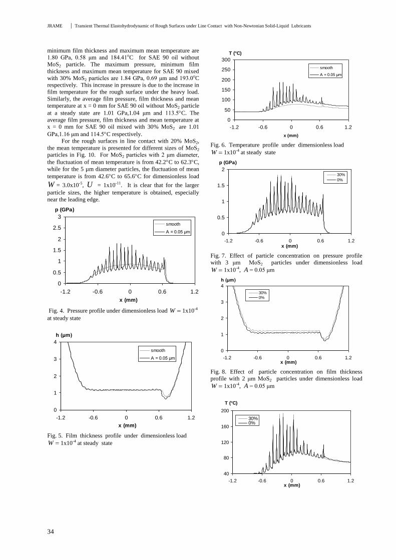
JRAME Transient Thermal Elastohydrodynamic of Rough Surfaces under Line Contact with Non-Newtonian Solid-Liquid Lubricants
34
minimum film thickness and maximum mean temperature are
1.80 GPa, 0.58 μm and 184.41oC for SAE 90 oil without
MoS2 particle. The maximum pressure, minimum film
thickness and maximum mean temperature for SAE 90 mixed
with 30% MoS2 particles are 1.84 GPa, 0.69 μm and 193.0oC
respectively. This increase in pressure is due to the increase in
film temperature for the rough surface under the heavy load.
Similarly, the average film pressure, film thickness and mean
temperature at x = 0 mm for SAE 90 oil without MoS2 particle
at a steady state are 1.01 GPa,1.04 μm and 113.5C. The
average film pressure, film thickness and mean temperature at
x = 0 mm for SAE 90 oil mixed with 30% MoS2 are 1.01
GPa,1.16 μm and 114.5C respectively.
For the rough surfaces in line contact with 20% MoS2,
the mean temperature is presented for different sizes of MoS2
particles in Fig. 10. For MoS2 particles with 2 μm diameter,
the fluctuation of mean temperature is from 42.2C to 62.3C,
while for the 5 µm diameter particles, the fluctuation of mean
temperature is from 42.6C to 65.6C for dimensionless load
W = 3.0x10⁻⁵, U = 1x10-11. It is clear that for the larger
particle sizes, the higher temperature is obtained, especially
near the leading edge.
p (GPa)
0
0.5
1
1.5
2
2.5
3
-1.2 -0.6 0 0.6 1.2
x (mm)
smooth
A = 0.05 μm
Fig. 4. Pressure profile under dimensionless load W 1x10⁻⁴
at steady state
h (μm)
0
1
2
3
4
-1.2 -0.6 0 0.6 1.2
x (mm)
smooth
A = 0.05 μm
Fig. 5. Film thickness profile under dimensionless load
W 1x10⁻⁴ at steady state
T (°C)
0
50
100
150
200
250
300
-1.2 -0.6 0 0.6 1.2
x (mm)
smooth
A = 0.05 μm
Fig. 6. Temperature profile under dimensionless load
W 1x10⁻⁴ at steady state
p (GPa)
0
0.5
1
1.5
2
-1.2 -0.6 0 0.6 1.2x (mm)
30%
0%
Fig. 7. Effect of particle concentration on pressure profile
with 3 μm MoS2 particles under dimensionless load
W 1x10⁻⁴, A = 0.05 μm
h (μm)
0
1
2
3
4
-1.2 -0.6 0 0.6 1.2x (mm)
30%
0%
Fig. 8. Effect of particle concentration on film thickness
profile with 2 μm MoS2 particles under dimensionless load
W 1x10⁻⁴, A = 0.05 μm
T (°C)
40
80
120
160
200
-1.2 -0.6 0 0.6 1.2x (mm)
30%0%
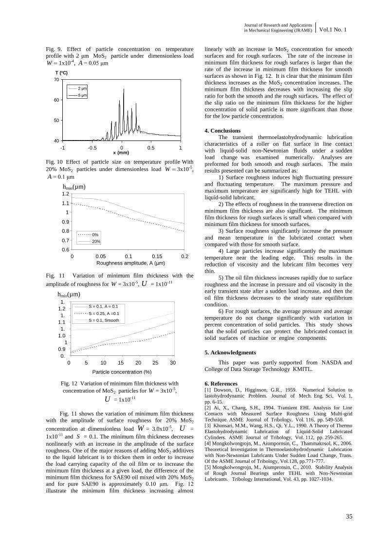
Journal of Research and Applications
in Mechanical Engineering (JRAME) Vol.1 No. 1
35
Fig. 9. Effect of particle concentration on temperature
profile with 2 μm MoS2 particle under dimensionless load
W 1x10⁻⁴, A = 0.05 μm
T (°C)
40
50
60
70
-1 -0.5 0 0.5 1x (mm)
2 μm
5 μm
Fig. 10 Effect of particle size on temperature profile With
20% MoS2 particles under dimensionless load W 3x10⁻⁵,
A = 0.1 μm
Fig. 11 Variation of minimum film thickness with the
amplitude of roughness for W = 3x10⁻⁵, U = 1x10-11
Fig. 12 Variation of minimum film thickness with
concentration of MoS2 particles for W = 3x10⁻⁵,
U = 1x10-11
Fig. 11 shows the variation of minimum film thickness
with the amplitude of surface roughness for 20% MoS2
concentration at dimensionless load W = 3.0x10⁻⁵, U =
1x10-11 and S = 0.1. The minimum film thickness decreases
nonlinearly with an increase in the amplitude of the surface
roughness. One of the major reasons of adding MoS2 additives
to the liquid lubricant is to thicken them in order to increase
the load carrying capacity of the oil film or to increase the
minimum film thickness at a given load, the difference of the
minimum film thickness for SAE90 oil mixed with 20% MoS2
and for pure SAE90 is approximately 0.10 μm. Fig. 12
illustrate the minimum film thickness increasing almost
linearly with an increase in MoS2 concentration for smooth
surfaces and for rough surfaces. The rate of the increase in
minimum film thickness for rough surfaces is larger than the
rate of the increase in minimum film thickness for smooth
surfaces as shown in Fig. 12. It is clear that the minimum film
thickness increases as the MoS2 concentration increases. The
minimum film thickness decreases with increasing the slip
ratio for both the smooth and the rough surfaces. The effect of
the slip ratio on the minimum film thickness for the higher
concentration of solid particle is more significant than those
for the low particle concentration.
4. Conclusions
The transient thermoelastohydrodynamic lubrication
characteristics of a roller on flat surface in line contact
with liquid-solid non-Newtonian fluids under a sudden
load change was examined numerically. Analyses are
preformed for both smooth and rough surfaces. The main
results presented can be summarized as:
1) Surface roughness induces high fluctuating pressure
and fluctuating temperature. The maximum pressure and
maximum temperature are significantly high for TEHL with
liquid-solid lubricant.
2) The effects of roughness in the transverse direction on
minimum film thickness are also significant. The minimum
film thickness for rough surfaces is small when compared with
minimum film thickness for smooth surfaces.
3) Surface roughness significantly increase the pressure
and mean temperature in the lubricated contact when
compared with those for smooth surface.
4) Large particles increase significantly the maximum
temperature near the leading edge. This results in the
reduction of viscosity and the lubricant film becomes very
thin.
5) The oil film thickness increases rapidly due to surface
roughness and the increase in pressure and oil viscosity in the
early transient state after a sudden load increase, and then the
oil film thickness decreases to the steady state equilibrium
condition.
6) For rough surfaces, the average pressure and average
temperature do not change significantly with variation in
percent concentration of solid particles. This study shows
that the solid particles can protect the lubricated contact in
solid surfaces of machine or engine components.
5. Acknowledgments
This paper was partly supported from NASDA and
College of Data Storage Technology KMITL.
6. References [1] Dowson, D., Higginson, G.R., 1959. Numerical Solution to lastohydrodynamic Problem. Journal of Mech. Eng. Sci, Vol. 1,
pp. 6-15.
[2] Ai, X., Chang, S.H., 1994. Transient EHL Analysis for Line
Contacts with Measured Surface Roughness Using Multi-grid
Technique. ASME Journal of Tribology, Vol. 116, pp. 549-558. [3] Khonsari, M.M., Wang, H.S., Qi, Y.L., 1990. A Theory of Thermo
Elastohydrodynamic Lubrication of Liquid-Solid Lubricated
Cylinders. ASME Journal of Tribology, Vol. 112, pp. 259-265. [4] Mongkolwongrojn, M., Aiumpornsin, C., Thammakosol, K., 2006.
Theoretical Investigation in Thermoelastohydrodynamic Lubrication
with Non-Newtonian Lubricants Under Sudden Load Change, Trans. Of the ASME Journal of Tribology, Vol.128, pp.771-777.
[5] Mongkolwongrojn, M., Aiumpronsin, C., 2010. Stability Analysis
of Rough Journal Bearings under TEHL with Non-Newtonian Lubricants. Tribology International, Vol. 43, pp. 1027-1034.
hmin(µm)
0.9
0.95
1 1.05
1.1
1.15
1.2
1.25
1.3
0%
5%
10%
15%
20%
25%
30%
Particle concentration (%)
S = 0.1, A = 0.1
S = 0.25, A =0.1 S = 0.1, Smooth
hmin(µm)
0.6
0.7
0.8
0.9
1
1.1
1.2
0 0.05 0.1 0.15 0.2 Roughness amplitude, A (µm)
0% 20%

JRAME Transient Thermal Elastohydrodynamic of Rough Surfaces under Line Contact with Non-Newtonian Solid-Liquid Lubricants
36
7. Nomenclature
A = Roughness amplitude (m)
iA = Contact area of an individual particle
b = Hertzian half-width (m), 0.5
8b R W
B = Width of rolling cylinders (m)
E = Equivalent modulus of elasticity (Pa)
PSE = Equivalent modulus of elasticity of particle
and rolling/sliding (Pa)
Pf = Friction coefficient of solid particle
h = Film thickness (m)
H = Dimensionless film thickness, 2H R b h
dH = Brinell hardness of particle (Pa)
0k = Thermal conductivity of lubricant
at ambient pressure (W/(m∙K))
pk = Dimensionless piezothermal conductivity
l = Wave length of roughness (m)
0m = viscosity consistency (Pa∙sn)
n = Power law index
xN = Number of particles in x-direction
zN = Number of particles in z-direction
p = Pressure (Pa)
HP = Maximum Hertzian pressure (Pa), 0.5
2HP E W
P = Dimensionless pressure, HP p P
R = Equivalent radius (m), 1
1 21 1R R R
S = Slide ratio, 2 1S u u u
t = Time (s)
*t = Dimensionless time, *t u b t
T = Temperature (K)
oT = Inlet temperature (K)
T = Dimensionless film temperature
u = Dimensionless velocity, u u u
u = Mean velocity (m/s), 1 2 2u u u
U = Dimensionless speed parameter, 0U u E R
w = Applied Load (N/m)
Pw = Load support by particle (N/m)
W = Dimensionless load parameter, 2W w E R
PW = Dimensionless load support by particle
,X Y =Dimensionless coordinate 2,x bX Y R b y H
lz = Viscosity-Pressure index
Greek
o = viscosity at ambient pressure (Pa∙s)
* = Equivalent viscosity (Pa∙s)
* = Dimensionless equivalent viscosity,
*
0
0 = Inlet density of oil (kg/m3)
= Dimensionless density, 0
f = Density of oil (kg/m3)
p = Density of particle (kg/m3)
1/ 2 = Density of roller / slider (kg/m3)
p = Poisson ratio of particles
s = Poisson ratio of rolling/slider
= Viscosity-Temperature coefficient (1/K)
= concentration of particles by weight
*ผตดตอ: E-Mail: [email protected], เบอรโทรศพท: (662) 329-8350-1, โทรสาร: (662) 329-8352
Vol. 1 No.1 TSME | Journal of Research and Applications in Mechanical Engineering
การจ าลองเชงตวเลขของการถายเทความรอนแบบลามนารในทอสเหลยมจตรสทมการตดตงแผนออรฟต Numerical Simulation of Laminar Heat Transfer in a Square Duct fitted
with Orifices
กตตราช สจวรยทรพย, พทกษ พรอมไธสง, กตธญ ค าพนยม และ พงษเจต พรหมวงศ*
สาขาวชาวศวกรรมเครองกล คณะวศวกรรมศาสตร สถาบนเทคโนโลยพระจอมเกลาเจาคณทหารลาดกระบง เขตลาดกระบง กรงเทพฯ 10520
บทคดยอ การวเคราะหเชงตวเลขแบบสามมตของการถายเทความรอนในชวงการไหลแบบลามนารในทอสเหลยมจตรสทมการตดตงแผนออรฟตท ามม ก าหนดใหผวทอมลกษณะแบบอณหภมทผวคงท โดยไดมการตดตงแผนออรฟตใหมลกษณะการจดวางเอยงท ามมปะทะท = 30o โดยมคาอตราสวนระหวางเสนผานศนยกลางของออรฟตตอเสนผานศนยกลางของทอ (diameter ratio (d/D), DR) เทากบ 0.5-0.8 และอตราสวนของระยะหางระหวางแผนออรฟตตอความสงของทอ (Pitch ratio, PR) เทากบ 1.5 การค านวณใชวธปรมาตรสบเนองและเลอกล าดบวธหาผลเฉลยแบบ SIMPLE ซงการจ าลองนไดน าเสนอคณลกษณะการถายเทความรอนและการไหลของของไหลส าหรบเลขเรยโนลดบนพนฐานเสนผานศนยกลางไฮดรอลกสของทอสเหลยมจตรส ชวงจาก Re = 100 ถง 1200 และไดศกษาผลของแผนออรฟตตอการถายเทความรอนและการสญเสยความดนในทอสเหลยมจตรส ผลลพธทไดจากทอสเหลยมจตรสทมการตดแผนออรฟตถกน าไปเปรยบเทยบกบทอสเหลยมจตรสผวเรยบ โดยคาการถายเทความรอนโดยแสดงในเทอมของเลขนสเซลท (Nusselt number) และการสญเสยความดนโดยแสดงในเทอมของตวประกอบเสยดทาน (friction factor) พบวาทอสเหลยมจตรสทมการตดแผนออรฟตชวยเพมการถายเทความรอนไดดกวาทอสเหลยมจตรสผวเรยบ และการลดลงของ DR ท าใหคาเลขนสเซลทและตวประกอบเสยดทานเพมขน โดยคา DR=0.5 จะใหคาการถายเทความรอนและคาความดนสญเสยมากทสด
ค าหลก: ทอจตรส, แผนออรฟต, การถายเทความรอน, ความเสยดทาน
Abstract
Laminar periodic flow and heat transfer in a three dimensional square channel with isothermal walls and with =30o
orifice baffle; (diameter ratio (d/D), DR) in range from 0.5 to 0.8 and (Pitch ratio, PR) of 1.5 is investigated numerically. The
computations based on the finite volume method, and the SIMPLE algorithm has been implemented. The fluid flow and heat
transfer characteristics are presented for Reynolds numbers based on the hydraulic diameter of the square channel ranging from
100 to 1200. Effects of orifice baffle on heat transfer and pressure loss in the square channel are studied. It is found that the
orifice baffle performs better than the smooth square channel for all Reynolds number values. The decrease of the DR leads to an
increase in the Nusselt number and friction factor. The computational results reveal that the DR of 0.5 provided the highest on
both heat transfer and friction factor.
Keywords: square channel, orifice baffle, heat exchanger, friction
1. บทน า การเพมขนของประสทธภาพในการแลกเปลยนความรอนเปนสง
ทจ าเปนอยางยงในการประยกตใชในในอปกรณดานอตสาหกรรมตาง ๆ ดงนนจงไดมการน าเทคนควธตาง ๆ เพอเปนการเพมคาการถายเทความรอนและเพมสมรรถนะการเพมการถายเทความรอน ตวอยางเทคนคทใชกนอยางแพรหลาย คอ การเพมการถายเทความรอนโดยอาศยการตดตงตวสรางการไหลแบบปนปวนทเรยกวา turbulators เชน ครบ ( ribs) [1], แผนขรขระหรอผวทอท มการเซาะรอง (grooves/dimples) [2], ปก (winglets) [3] และแผนกน (baffles) [4] โดยตวสรางการไหลปนปวนนถกน ามาใชเพอเปนการกอกวนการไหล
ท าใหเกดการหมนวนของการไหลแนวยาวและเพมการผสมใหดยงขน ซงวธการเพมการถายเทความรอนนไดมการน ามาประยกตใชทางดานวศวกรรมในสายงานตาง ๆ เชน เครองแลกเปลยนความรอนทมขนาดกะทดรด เครองท าอากาศเยนจากแผงรบแสงอาทตย และแผงระบายความรอนอปกรณอเลกทรอนกส
เนองจากระบบการแลกเปลยนความรอนเปนระบบทส าคญส าหรบโรงงานอตสาหกรรมตาง ๆ ดงน นจงไดมความสนใจในการศกษาในสวนของการเพมการแลกเปลยนความรอนและพฤตกรรมการไหลรวมถงคาความดนสญเสยทเกดขนโดยมการศกษาทงในสวนของการใชการทดลองและในสวนของการศกษาโดยใชวธเชงตวเลข
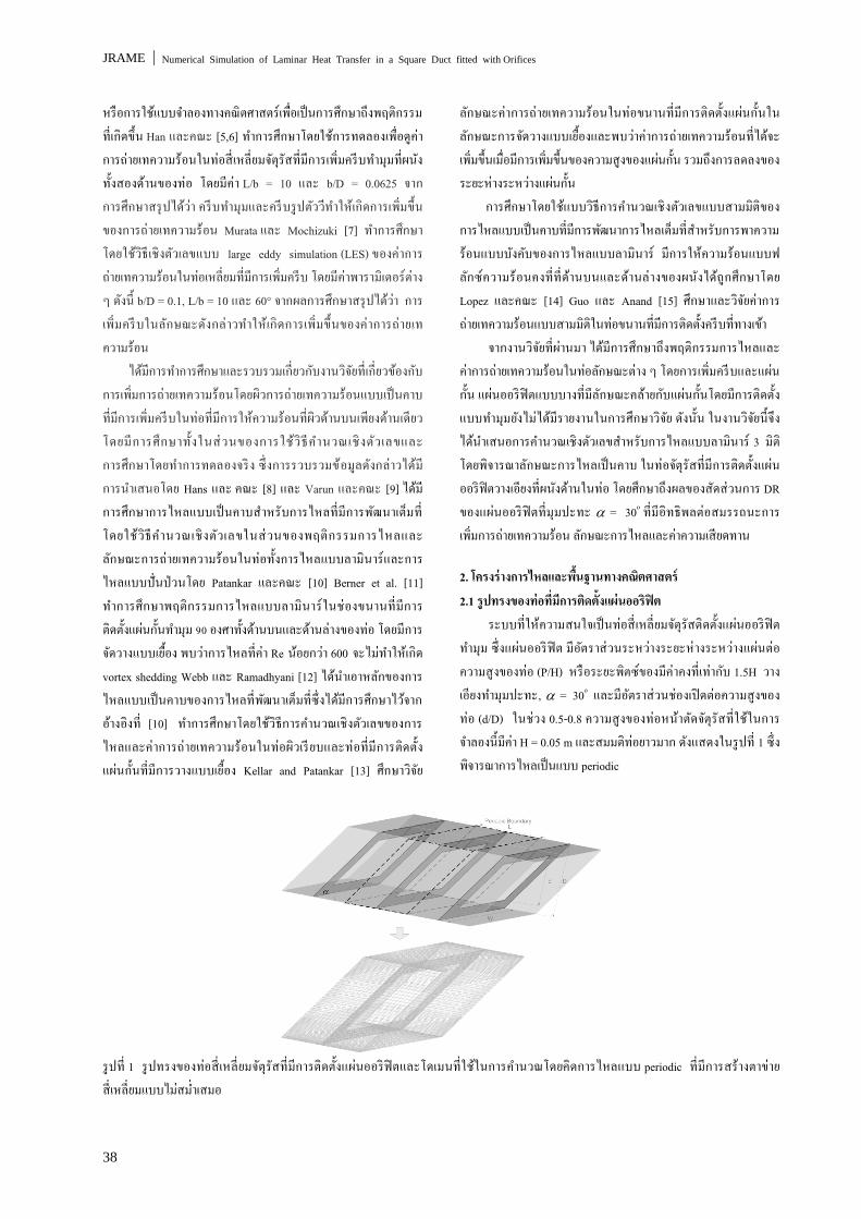
JRAME Numerical Simulation of Laminar Heat Transfer in a Square Duct fitted with Orifices
38
หรอการใชแบบจ าลองทางคณตศาสตรเพอเปนการศกษาถงพฤตกรรมทเกดขน Han และคณะ [5,6] ท าการศกษาโดยใชการทดลองเพอดคาการถายเทความรอนในทอสเหลยมจตรสทมการเพมครบท ามมทผนงทงสองดานของทอ โดยมคา L/b = 10 และ b/D = 0.0625 จากการศกษาสรปไดวา ครบท ามมและครบรปตววท าใหเกดการเพมขนของการถายเทความรอน Murata และ Mochizuki [7] ท าการศกษาโดยใชวธเชงตวเลขแบบ large eddy simulation (LES) ของคาการถายเทความรอนในทอเหลยมทมการเพมครบ โดยมคาพารามเตอรตาง ๆ ดงน b/D = 0.1, L/b = 10 และ 60° จากผลการศกษาสรปไดวา การเพมครบในลกษณะดงกลาวท าใหเกดการเพมขนของคาการถายเทความรอน
ไดมการท าการศกษาและรวบรวมเกยวกบงานวจยทเกยวของกบการเพมการถายเทความรอนโดยผวการถายเทความรอนแบบเปนคาบทมการเพมครบในทอทมการใหความรอนทผวดานบนเพยงดานเดยว โดยมการศกษาท งในสวนของการใชว ธค านวณเชงตวเลขและการศกษาโดยท าการทดลองจรง ซงการรวบรวมขอมลดงกลาวไดมการน าเสนอโดย Hans และ คณะ [8] และ Varun และคณะ [9] ไดมการศกษาการไหลแบบเปนคาบส าหรบการไหลทมการพฒนาเตมทโดยใชวธค านวณเชงตวเลขในสวนของพฤตกรรมการไหลและลกษณะการถายเทความรอนในทอทงการไหลแบบลามนารและการไหลแบบปนปวนโดย Patankar และคณะ [10] Berner et al. [11] ท าการศกษาพฤตกรรมการไหลแบบลามนารในชองขนานทมการตดตงแผนกนท ามม 90 องศาทงดานบนและดานลางของทอ โดยมการจดวางแบบเยอง พบวาการไหลทคา Re นอยกวา 600 จะไมท าใหเกด vortex shedding Webb และ Ramadhyani [12] ไดน าเอาหลกของการไหลแบบเปนคาบของการไหลทพฒนาเตมทซงไดมการศกษาไวจากอางองท [10] ท าการศกษาโดยใชวธการค านวณเชงตวเลขของการไหลและคาการถายเทความรอนในทอผวเรยบและทอทมการตดตงแผนกนทมการวางแบบเยอง Kellar and Patankar [13] ศกษาวจย
ลกษณะคาการถายเทความรอนในทอขนานทมการตดตงแผนกนในลกษณะการจดวางแบบเยองและพบวาคาการถายเทความรอนทไดจะเพมขนเมอมการเพมขนของความสงของแผนกน รวมถงการลดลงของระยะหางระหวางแผนกน
การศกษาโดยใชแบบวธการค านวณเชงตวเลขแบบสามมตของการไหลแบบเปนคาบทมการพฒนาการไหลเตมทส าหรบการพาความรอนแบบบงคบของการไหลแบบลามนาร มการใหความรอนแบบฟลกซความรอนคงททดานบนและดานลางของผนงไดถกศกษาโดย Lopez และคณะ [14] Guo และ Anand [15] ศกษาและวจยคาการถายเทความรอนแบบสามมตในทอขนานทมการตดตงครบททางเขา
จากงานวจยทผานมา ไดมการศกษาถงพฤตกรรมการไหลและคาการถายเทความรอนในทอลกษณะตาง ๆ โดยการเพมครบและแผนกน แผนออรฟตแบบบางทมลกษณะคลายกบแผนกนโดยมการตดตงแบบท ามมยงไมไดมรายงานในการศกษาวจย ดงนน ในงานวจยนจงไดน าเสนอการค านวณเชงตวเลขส าหรบการไหลแบบลามนาร 3 มต โดยพจารณาลกษณะการไหลเปนคาบ ในทอจตรสทมการตดตงแผนออรฟตวางเอยงทผนงดานในทอ โดยศกษาถงผลของสดสวนการ DR ของแผนออรฟตทมมปะทะ = 30o ทมอทธพลตอสมรรถนะการเพมการถายเทความรอน ลกษณะการไหลและคาความเสยดทาน
2. โครงรางการไหลและพนฐานทางคณตศาสตร 2.1 รปทรงของทอทมการตดตงแผนออรฟต
ระบบทใหความสนใจเปนทอสเหลยมจตรสตดตงแผนออรฟตท ามม ซงแผนออรฟต มอตราสวนระหวางระยะหางระหวางแผนตอความสงของทอ (P/H) หรอระยะพตซของมคาคงทเทากบ 1.5H วางเอยงท ามมปะทะ, = 30o และมอตราสวนชองเปดตอความสงของทอ (d/D) ในชวง 0.5-0.8 ความสงของทอหนาตดจตรสทใชในการจ าลองนมคา H = 0.05 m และสมมตทอยาวมาก ดงแสดงในรปท 1 ซงพจารณาการไหลเปนแบบ periodic
รปท 1 รปทรงของทอสเหลยมจตรสทมการตดตงแผนออรฟตและโดเมนทใชในการค านวณโดยคดการไหลแบบ periodic ทมการสรางตาขายสเหลยมแบบไมสม าเสมอ

Journal of Research and Applications
in Mechanical Engineering (JRAME) Vol.1 No. 1
39
2.2 พนฐานทางคณตศาสตร การพฒนาแบบจ าลองเชงตวเลขส าหรบการไหลของของไหล
และการถายเทความรอนในทอสเหลยมจตรส โดยมสมมตฐานดงตอไปน - การไหลของของไหลและการถายเทความรอนเปนแบบคงตว 3 มต - การไหลเปนแบบลามนารและเปนแบบอดตวไมได - คณสมบตของของไหลคงท - ไมค านงแรงวตถและการสญสลายเนองจากความหนด - ไมค านงการแผรงสความรอน จากสมมตฐานขางตน ส าหรบการไหลในทอสเหลยมจตรสสมการควบคมประกอบไปดวยสมการความตอเนอง สมการนาเวยร-สโตก และสมการพลงงาน สามารถเขยนในรปเทนเซอรในระบบพกดคารทเซยนดงน
สมการความตอเนอง:
0
i
i
ux
(1)
สมการโมเมนตม:
i
j
j
i
jij
ji
x
u
x
u
xx
p
x
uu
(2)
สมการพลงงาน:
jj
i
i x
T
xTu
x (3)
เมอ คอ การแพรทางความรอน ก าหนดโดย
Pr
(4)
สมการควบคมท งหมดจะถกดสเครทไทซโดยแบบแผนวธผลตางครอดราตค(Quadratic upstream interpolation for convective kinetics differencing scheme, QUICK) แลวท าการค านวณหาผลเฉลยตามระเบยบวธปรมาตรสบเนอง [16] โดยแผนผงวธแบบ SIMPLE (Semi-implicit method for pressure-linked equations) ในการลเขาหาค าตอบจะพจารณาทความแตกตางของคาการแปรเปลยนนอยกวา 10-5 ของทกตวแปร
ในงานวจยนมตวแปรทใหความสนใจอย 4 ตวแปร คอ เลขเรยโนลด ตวประกอบเสยดทาน เลขนสเซลท และ สมรรถนะเชงความรอน ซงคาเลขเรยโนลดนยามโดย
/Re hDu (5) ตวประกอบเสยดทาน, f ค านวณไดจากความดนตกครอม, p ตลอดชวงความยาว periodic ของทอสเหลยมจตรส, L
2)2/1(
/
u
DLpf h
(6)
การถายเทความรอนค านวณหาจากคาเลขนสเซลทเฉพาะท ซงสามารถเขยนไดเปน
k
DhNu hx
x (7)
คาเลขนสเซลทเฉลยสามารถค านวณไดจาก
ANuA
Nu x
1 (8)
สมรรถนะเชงความรอน, 3/1
00 /// ffNuNu (9) เมอ Nu0 และ f0 คอ เลขนสเซลทและตวประกอบเสยดทานของทอผวเรยบ ตามล าดบ
ส าหรบการไหลในทอจตรสน โดเมนทใชในการค านวณหาผลเฉลยเปนเอลเมนตรปทรงสเหลยมและแบงกรดแบบไมสม าเสมอ (Non-uniform grid) การหาผลกระทบของกรดทมผลตอค าตอบ ไดท าการเปรยบเทยบผลเฉลยโดยใชจ านวนของกรดทแตกตางกน คอ ท 80,000 และ 160,000 พบวาเมอขนาดเพมขนเปน 160,000 คาเลขนสเซลทเปลยนแปลงนอยกวา 1.5% ดงนนจงเลอกจ านวนกรดเทากบ 80,000 ไปใชในการศกษาอทธพลของคาพารามเตอรตาง ๆ ตอไป
2.3 เงอนไขขอบ พจารณาทางเขาและทางออกเปนแบบ periodic translation สมมตอากาศท 300 K และมคาเลขพรานด 0.7 ไหลเขาดวยอตราการไหลเชงมวลคงท รปรางความเรวทางเขาและทางออกเหมอนกน สมมตคณสมบตทางกายภาพของอากาศมคาคงท โดยอางองทอณหภมเฉลยททางเขา เ งอนไขขอบเขตไมมการลนไถลทผนง (no-slip conditions) หรอความเรวทผนงมคาเทากบศนย เปนผนงทอยกบท (stationary wall) ก าหนดใหทผนงทกดานของทอจตรสมอณหภมผวคงท 310 K และสมมตใหแผนออรฟตเปนแผนกนความรอนไมสามารถผานได 3. ผลการทดลองและวจารณผล 3.1 การพสจนความถกตองของทอจตรสผวเรยบ
(a)
(b)
รปท 2 การตรวจสอบความถกตองของ (a) เลขนสเซลท (b) ตวประกอบเสยดทานของทอสเหลยมจตรสผวเรยบ
ในการพสจนความถกตองของการถายเทความรอนและตวประกอบเสยดทานในทอจตรสผวเรยบทไมมการเพมการตดตงแผนออ

JRAME Numerical Simulation of Laminar Heat Transfer in a Square Duct fitted with Orifices
40
รฟต โดยท าการเปรยบเทยบระหวางคาทไดจากวธเชงตวเลขและผลเฉลยแมนตรงภายใตเ งอนไขเดยวกนน ซงคาผลเฉลยแมนตรงนสามารถศกษาไดจากอางอง [17] โดยพบวาคาทไดจากวธเชงตวเลขจะมความคลาดเคลอนจากผลเฉลยแมนตรงประมาณ 0.5% ทงในสวนของคาเลขนสเซลทและคาตวประกอบเสยดทาน ซงผลลพธทไดโดยวธเชงตวเลขทงมความสอดคลองกนกบผลเฉลยแมนตรงอยางดและมความนาเชอถอได 3.2 โครงสรางการไหล
โครงสรางของการไหลในทอสเหลยมจตรสทตดตงแผนออรฟตท ามมปะทะ 30o ทคาสดสวน d/D, DR = 0.7 และ Re = 800 จากรปท 3 แสดงเวกเตอรของการไหลผานแผนออรฟต พบวาการเพมแผนออรฟตท าใหเกดการหมนวนและการกระแทกทผนงทอของกระแสการไหล เมออากาศไหลผานแผนออรฟตจะเกดการหมนวนทดานหลงของแผนออรฟตและเกดการกระแทกของกระแสการไหลทบรเวณผนงทงสดานของทอ โดยเฉพาะบรเวณดานหลงของแผนออรฟตทจะมการเหนยวน าท าใหเกดการกระแทกของกระแสซงสวนนเปนสวนส าคญทท าใหเกดการเพมการถายเทความรอน โดยแกนการไหลจะมการเปลยนต าแหนงแตกตางกนออกไปดงรป ซงแกนการไหลจะมต าแหนงทเปลยนแปลงตาม หนาตด A1 ถง A5 จากหนาตดดงกลาวจะสงเกตเหนทงในสวนของแกนการไหลของกระแสหลก และกระแสยอยทหมนวนในสวนของมมของทอ
รปท 3 เวกเตอรส าหรบการไหลในทอสเหลยมจตรสท Re = 800 และ DR = 0.7
3.3 การถายเทความรอน จากรปท 4 แสดงคอนทวรหรอการกระจายของสนามอณหภม
ส าหรบแผนออรฟตวางเอยงทคา Re = 800 และ DR = 0.7 ซงพบวาบรเวณชนชดผวความรอนทจะบางกวากรณทอผวเรยบซงแสดงใหเหนวาการตดตงแผนออรฟตท ามมจะท าใหเกดการกอกวนบรเวณชนชดผว ซงสงผลใหการถายเทความรอนระหวางอากาศและผนงมอตราทสงขน จากรปแสดงใหเหนไดวาบรเวณผนงดานขางทงสองดานจะมชนชดผวความรอนทบางมากกวาผนงดานบนและลาง ซงกรณการเพมแผนออรฟต DR = 0.5 ใหการถายเทความรอนทบรเวณผนงสงกวา
กรณอน ๆ ในทกกรณททดสอบ เนองจากกรณนจะท าใหเกดกระแสการไหลทมการกระแทกสงทสด
รปท 5 แสดงคอนทวรหรอการกระจายตวของเลขนสเซลทส าหรบแผนออรฟตวางเอยงทคา Re = 800 และ DR = 0.7 พบวาเกดการกระแทกทผนงทงสดานของทอท าใหมอตราการถายเทความรอนเพมมากขน โดยสวนทมการแสดงคอนทวรสแดงจะเปนสวนทมการเกดการกระแทกของกระแสการไหลมากทสดซงจะเกดทบรเวณดานบนและดานลางของทอ
รปท 6 แสดงการแปรเปลยนคาอตราสวนเลขนสเซลทกบเลขเรยโนลด ของแผนออรฟตวางเอยงท ามมปะทะ 30o ทคา DR ตาง ๆ จากกราฟ พบวาเมอคา DR ลดลง ท าใหคาเลขนสเซลทเพมมากขน โดย DR = 0.5 จะใหคาเลขนสเซลทมากทสด โดยมคาเลขนสเซลทเทากบ 10 เทาเมอเทยบกบทอผวเรยบ โดยในการใชแผนออรฟตทมคา DR = 0.5-0.8 จะใหคาการเพมการถายเทความรอนอยในชวง 1-10 เทาเมอเทยบกบทอผวเรยบ
รปท 4 ภาพตดคอนทวรอณหภมบนระนาบขวางการไหล ในต าแหนงตาง ๆ ของทอจตรสทตดตงแผนออรฟต ส าหรบ Re = 800 และ DR = 0.7
รปท 5 ภาพตดคอนทวรเลขนสเซลท ของทอจตรสทตดตงแผนออรฟต ส าหรบ Re = 800 และ DR=0.7
รปท 6 การแปรเปลยนของคาอตราสวนเลขนสเซลทกบเลขเรยโนลดของแผนออรฟตวางเอยงท ามมปะทะ 30o ทคา DR ตาง ๆ

Journal of Research and Applications
in Mechanical Engineering (JRAME) Vol.1 No. 1
41
3.4 การสญเสยความดน รปท 7 แสดงความสมพนธระหวางเลขเรยโนลดกบอตรา
สวนตวประกอบเสยดทานระหวางทอจตรสตดแผนออรฟตตอทอจตรสผวเรยบ, (f/f0) ทคา DR ตาง ๆ ซงเมอพจารณาชวงเลขเรยโนลดระหวาง 100 ถง 1200 พบวาคาเลขเรยโนลดทเพมขนมผลท าใหอตราสวนตวประกอบเสยดทานเพมขนตาม และเมอท าการเพมคา DR ท าใหคาอตราสวนตวประกอบเสยดทานมคาลดลง กรณแผนออรฟตวางเอยงท ามมปะทะ 30o ท DR = 0.5 มอตราการเพมคาอตราสวนตวประกอบเสยดทานสงทสด โดยใหคาเปน 100 เทาของทอผวเรยบ จากกราฟสรปไดวาการตดตงแผนออรฟตท ามม โดยมคา DR = 0.5-0.8 จะใหคาตวประกอบเสยดทานอยในชวง 1-100 เทาเมอเทยบกบทอผวเรยบ
รปท 7 การแปรเปลยนของคาอตราสวนตวประกอบเสยดทานของแผนออรฟตวางเอยงท ามมปะทะ 30o ทคา DR ตาง ๆ
3.5 สมรรถนะการเพมการถายเทความรอน รปท 8 แสดงความแปรเปลยนคาสมรรถนะการเพมการถายเท
ความรอนทคาเลขเรยโนลดตาง ๆ ของทอจตรสตดตงแผนออรฟตท ามม โดยมคา DR = 0.5-0.8 พบวาคาเลขเรยโนลดทเพมสงขนมผลตอการเพมขนของสมรรถนะเชงความรอนในชวงเลขเรยโนลดทพจารณา โดยคา DR = 0.6 จะใหคาสมรรถนะเชงความรอนทสงทสดทท าการพจารณา โดยมคาเทากบ 2.2 ทคาเลขเรยโนลดเทากบ 1200 คาสมรรถนะเชงความรอนทไดจากการตดตงแผนออรฟตทม DR = 0.5-0.8 จะมคาอยในชวง 0.9-2.2
รปท 8 การแปรเปลยน ของแผนออรฟตวางเอยงท ามมปะทะ 30o ทคา DR ตาง ๆ
4. สรปผลการทดลอง จากผลการทดลองขางตนสามารถสรปไดวา ทอสเหลยมจตรสม
การตดตงแผนออรฟตเอยงท ามมปะทะ 30o โดยมคา DR = 0.5-0.8 จะชวยเพมการถายเทความรอน 1 เทา ถง 10 เทา, มความเสยดทานเพมขน 1 ถง 100 เทา เมอเปรยบเทยบกบทอสเหลยมจตรสผวเรยบและใหคาสมรรถนะการถายเทความรอนอยในชวง 0.9-2.2 ส าหรบทอจตรสทตดตงแผนออรฟตท ามม พบวาคา DR = 0.5 จะใหคาการเพมการถายเทความรอนและคาตวประกอบเสยดทานสงทสด สวนคา DR = 0.6 จะใหคาสมรรถนะการเพมการถายเทความรอนมากทสดทคาเลขเรยโนลดเทากบ 1200 ซงเปนเลขเรยโนลดทสงทสดทท าการพจารณา
5. เอกสารอางอง [1] Promvonge, P., Thianpong, C., 2008. Thermal performance assessment of turbulent channel flow over different shape ribs. Int.
Commun. Heat Mass Transfer, Vol. 35, No.10, pp. 1327–1334.
[2] Ridouane, E.H., Campo, A., 2008. Heat transfer enhancement of air flowing across grooved channels:joint effects of channel
height and groove depth. ASME J. Heat Transfer , Vol. 130, No.2,
[3] Chompookham, T., Thianpong, C., Kwankaomeng, S., Promvonge, P., 2010. Heat transfer augmentation in a wedge-ribbed
channel using winglet vortex generators. Int. Commun. Heat Mass
Transfer, Vol. 37, No. 2, pp. 163-169. [4] Sripattanapipat, S., Promvonge, P, 2009. Numerical analysis of
laminar heat transfer in a channel with diamond-shaped baffles. Int.
Commun. Heat Mass Transfer, Vol. 36, No. 1, pp. 32-38. [5] Han, J.C., Zhang, Y.M., Lee, C.P., 1991. Augmented heat
transfer in square channels with parallel. crossed and V-shaped
angled ribs. ASME J. Heat Transfer, Vol. 113, pp. 590–596. [6] Han, J.C., Zhang, Y.M., Lee, C.P., 1992. Influence of surface
heat flux ratio on heat transfer augmentation in square channels with
parallel, crossed, and V-shaped angled ribs. ASME J.
Turbomachinery, Vol. 114, pp. 872–880.
[7] Murata, A., Mochizuki, S., 2001. Comparison between laminar
and turbulent heat transfer in a stationary square duct with transverse or angled rib turbulators. Int. J. Heat Mass Transfer, Vol. 44, pp.
1127–1141.
[8] Hans, V.S., Saini, R.P., Saini, J.S., 2009. Performance of artificially roughened solar air heaters–A review. Renewable and
Sustainable Energy Reviews, Vol. 13, pp. 1854–1869. [9] Varun, Saini., R.P., Singal, S.K,. 2007. A review on roughness
geometry used in solar air heaters. Solar Energy, Vol. 81, pp. 1340–
1350. [10] Patankar, S.V., Liu, C.H., Sparrow, E.M., 1977. Fully
developed flow and heat transfer in ducts having streamwise-
periodic variations of cross-sectional area. ASME J. Heat Transfer, Vol. 99, pp. 180-186.
[11] Berner, C., Durst, F., McEligot, D.M., 1984. Flow around
baffles. Trans. ASME J. Heat Transfer, Vol. 106, pp. 743–749. [12] Webb, B.W., Ramadhyani, S., 1985. Conjugate heat transfer in
a channel with staggered ribs. Int. J. Heat Mass Transfer, Vol. 28,
pp. 1679–1687.
[13] Kelkar, K.M., Patankar, S.V., 1987. Numerical prediction of
flow and heat transfer in a parallel plate channel with staggered fins.
ASME J. Heat Transfer, Vol. 109, pp. 25–30. [14] Lopez, J.R., Anand, N.K., Fletcher, L.S., 1996. Heat transfer in
a three-dimensional channel with baffles. Numerical Heat Transfer,
Part A: Applications, Vol. 30, pp. 189–205. [15] Guo, Z., Anand, N.K., 1997. Three-dimensional heat transfer
in a channel with a baffle in the entrance region. Numerical Heat
Transfer, Part A: Applications, Vol. 31, No. 1, pp. 21-35. [16] Patankar, S.V., 1980. Numerical Heat Transfer and Fluid Flow.
McGraw-Hill, New York.
[17] Incropera, F., Dewitt, P.D., 1996. Introduction to heat transfer.
3rd edition John Wiley & Sons Inc.

Vol. 1 No.1 TSME | Journal of Research and Applications in Mechanical Engineering
การท างานแบบมาสเตอร-สเลฟ ระหวางแขนกลแฮปตค 6 องศาอสระ โครงสรางแบบขนาน และ แขนกลลกผสมแบบขนาน 5 แกนตระกล เอช-4
Master-Slave Operation for a 6-DOF Parallel Haptic Device and
a Hybrid 5-Axis H-4 Family Parallel Manipulator
เรองยศ อารยวงษกล1 และ วบลย แสงวระพนธศร 2
1 , 2 ภาควชาวศวกรรมเครองกล คณะวศวกรรมศาสตร จฬาลงกรณมหาวทยาลย ถ.พญาไท ปทมวน กรงเทพมหานคร 10330. E-mail: [email protected], [email protected], 0-2218-6610-1, โทรสาร 0-2252-8889
บทคดยอ
งานวจยนเปนการน าเสนอระบบการท างานแบบมาสเตอร-สเลฟ ส าหรบสรางชนงานแบบกด แขนหนยนตทท างานแบบมาสเตอร-สเลฟทพฒนาขนนประกอบดวยแขนกลแฮปตค 6 องศาอสระโครงสราง แบบขนานท าหนาทเปนแขนกลน าหรอมาสเตอร และแขนกลลกผสมทมโครงสรางแบบขนาน 5 แกนตระกลเอช-4 ท าหนาทเปนแขนกลตามหรอสเลฟ การพฒนาระบบแขนกลน มจดมงหมายเพอใหสามารถท างานรวมกบผด าเนนการในการสรางชนงานทจดใหเปนการสรางชนงานตนแบบอยางเรวดวยวธการกดชนงานแบบ 5 แกน โดยแขนกลแฮปตคจะท าการเกบขอมลต าแหนงพนผวของชนงานทตองการท าซ า จากนนจงสงขอมลต าแหนงดงกลาวไปยงระบบควบคมแขนกลตามเพอใหแขนกลตามเคลอนทตามต าแหนงทบนทกจากแขนกลน าและท าการกดเซาะชนงาน
งานวจยนไดท าการทดสอบการเคลอนทและความสามารถในการสรางแรงสะทอนกลบไปยงมอของ ผควบคมแขนกลน าทเปนแขนกล แฮปตคทสรางขน พบวาผด าเนนการสามารถควบคมการท างานของระบบแขนกลไดดและแรงสะทอนกลบทเกดขนสงผลตอความรสกทมอของผ ควบคมในขณะกดชนงานอยางมนยส าคญ สวนการปรบปรงแขนกลตามเพอใหสามารถกดเซาะชนงานวสดไม และ โฟม พบวาชนงานทกดไดจากแขนกลตามมขนาดผดพลาดในระดบ 1 มลลเมตรซงเปนขอจ ากดของความสามารถในการวดของอปกรณตรวจรทตดตง ในแขนกลทงสอง
ค าหลก: แฮปตค / ชนงานตนแบบ / แรงสะทอนกลบ
Abstract
This paper illustrates a master-slave operation, for material removal processes, using in part prototyping processes which
are consisted of a 6-DOF parallel haptic device as a master arm and a hybrid 5-Axis H-4 family parallel manipulator as a slave
arm. The master-slave system is designed and built for 5-axis milling processes and aimed to use in a man-machine interfaced for
material removal processes of rapid prototyping system. The haptic arm or the master arm with force reflection capability is used
for measuring of 3D surface information, points and orientations, of the referenced object. The measured coordinates are used as
reference information to control positions and orientations of the end-effector of the slave manipulator arm, a 5-Axis machine.
The experimental results show that the operator with feeling of force, by operating the haptic device, can better control of the
slave manipulator arm in material removal processes. Force reflection information improves the feeling of operation significantly.
The results also show good accuracy with average error about 1 mm due to the limitation of the measurement sensors attached.
Keywords: Haptic / Master-Slave / Parallel Manipulator
1. บทน า งานวศวกรรมยอนกลบ (reverse engineering)และ งานสรางตน
แบบอยางเรว (rapid prototyping) มประโยชนตอภาคอตสาหกรรมอยางมาก แตในขณะเดยวกนผด าเนนงานกตองอาศยทกษะ ความรและความช านาญดานตางๆ เชน การวดขนาดดวยเครองวด CMM การท างานกบเครอง CNC และ การใชโปรแกรมดาน CAD/CAM เมอพจารณางานวศวกรรมยอนกลบพบวามขนตอนการท างานเรมจากการ
วดขนาดของชนงานตนแบบดนเหนยวหรอชนงานทตองการท าซ าแลวจงน าพกดของชนงานทวดไดไปสรางแบบสามมตในคอมพวเตอรดวยโปรแกรมดาน CAD และ ใชโปรแกรมดาน CAM เพอสรางเสนทางการกดชนงานดวยเครอง CNC ตอไป สวนการสรางชนงานตนแบบอยางเรวจะอาศยแบบสามมตทไดจากโปรแกรมดาน CAD แลวจงน าไปใชกบการสรางชนงานดวยเครองสรางตนแบบอยางเรว

JRAME Master-Slave Operation for a 6-DOF Parallel Haptic Device and a Hybrid 5-Axis H-4 Family Parallel Manipulator
44
ขนตอนการท างานดงทไดกลาวมานนตองอาศยระยะเวลาในการด าเนนการคอนขางมากเนองจาก จดพกดของผวชนงานทวดไดจากสวนของงานวศวกรรมยอนกลบนนยงไมสามารถน าไปสรางเสนทางเดนของเครอง CNC โดยตรง แตตองผานกระบวนการสรางแบบสามมตและการปรบแตงพนผวดวยโปรแกรมทางดาน CAD กอน ดงนนผวจยจงไดน าเสนอแนวทางเพอการแกปญหาดงกลาวโดยการใชระบบแขนกลซงประกอบดวยแขนกลน าและ แขนกลตามท าหนาทเรมตงแตการวดขนาดของชนงานจนกระทงท าการกดชนงานตามแบบทตองการไปพรอมๆกน
2. แขนกลน า (Master Arm) แขนกลน าทไดพฒนาขนมาแสดงไวในรปท 1 เปนแขนกล
แฮปตค 6 องศาอสระโครงสรางแบบขนานแบงโครงสรางเปน 3 แขน แตละแขนมลกษณะเหมอนกนและมฐานวางต าแหนงท ามมกน 120 องศา แขนทงสามเชอมตอไปยงดามจบดวยขอตอแบบ ยนเวอรแซล (universal) อปกรณหลกของแตละแขนประกอบดวย อปกรณวดมม (Encoder) จ านวน 3 ตว และ มอเตอรซงท าหนาทเปนอปกรณขบเพอสรางแรงกระท าตอมอผด าเนนการจ านวน 2 ตว ดงในรปท 2
ต าแหนงการเคลอนทและทศทางของปลายแขนกลน าสามารถหาจากสมการฟอรเวอรดคเนเมตคหากเราทราบต าแหนงการหมนของอปกรณวดมมทงหมด 9 ตว เพอใหสะดวกตอการพจารณา ในขนตอนการวเคราะหฟอรเวรดคเนเมตคจงไดแสดงภาพแขนกลน าโดยหมนภาพกลบขนมาในแนวตง ดงรปท 3
รปท 1 โครงสรางของแขนกลน า
รปท 2 โครงสรางแตละแขนของแขนกลน า
รปท 3 การก าหนดต าแหนงแกนบนโครงสราง
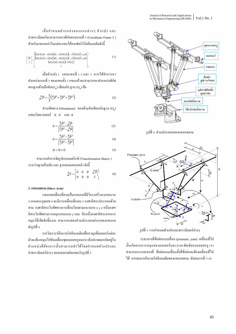
Journal of Research and Applications
in Mechanical Engineering (JRAME) Vol.1 No. 1
45
เ ม อก าหนดต าแห นงของแกนตางๆ ตวแปร และ คาพารามเตอรจะสามารถหาพกดของแกนท 5 (Coordinate Frame 5 ) ส าหรบแขนกลน าในแตละแขนไดจากฟอรเวรดคเนเมตคดงน
1
1 242432
121421431321
121421431321
5
iiiiiii
ib
iiiiiiiiiiii
ib
iiiiiiiiiiii
iB
cθL+dcθ+cθsθcθsθ
srssdLcsssscccs
crscdLcscsssccc
P
(1)
เมอตวแปร i แทนแขนท 1 2 และ 3 หากไดท าการหาต าแหนงแกนท 5 ของแขนทง 3 แขนแลวจะสามารถหาต าแหนงพกดของฐานดามมอจบ(OM) เทยบกบ ฐาน (OB) คอ
35
25
15
3
1PPPP BBBB
M
(2)
สวนทศทาง (Orientation) ของดามจบเทยบกบฐาน (OB) แสดงโดยเวกเตอร on
และ a
PP
PPn
BM
B
BM
B
15
15 (3)
3
52
5
35
25
PP
PPo
BB
BB
(4)
ona
(5)
สามารถท าการจดรปแบบเมตรกซ (Transformation Matrix ) ระหวางฐานดามจบ และ ฐานของแขนกลน า ดงน
1000
PaonT
BMB
M
(6)
3. แขนกลตาม (Slave Arm) แขนกลเคลอนทตามเปนแขนกลทมโครงสรางแบบขนาน
5 แกนตระกลเอช-4 จะมการเคลอนทแบบ 5 องศาอสระประกอบดวยสาม องศาอสระในทศทางการเลอนไถลตามแนวแกน x y z หนงองศาอสระในทศทางการหมนรอบแกน y และ อกหนงองศาอสระจากการหมนโตะยดจบชนงาน สามารถแสดงสวนประกอบตางๆของแขนกลดงรปท 4
การวเคราะหอนเวอรสคเนเมตคเพอหามมทมอเตอรแตละตวจะตองหมนไปขบเคลอนชดบอลสกรจนกระทงปลายดอกกดอยในต าแหนงทตองการน นสามารถท าไดโดยก าหนดตวแปรและคาพารามเตอรตางๆ ของแขนกลดงแสดงในรปท 5
รปท 4 สวนประกอบของแขนกลตาม
รปท 5 การก าหนดตวแปรและพารามเตอรตางๆ
ระยะทางทขอตอแบบเลอน (prismatic joint) เคลอนทไปนนเกดจากการหมนของมอเตอรและระยะพตซของบอลสกร เราสามารถหาระยะทางท ขอตอแบบเลอนทงสขอตอจะตองเคลอนทไปได จากสมการอนเวอรสคเนเมตคของแขนกลตาม ดงสมการท 7-10

JRAME Master-Slave Operation for a 6-DOF Parallel Haptic Device and a Hybrid 5-Axis H-4 Family Parallel Manipulator
46
2
2
2
1
cos2
cossin
sincos
sin2
2
1
1
2
1
1
1
gedcTh
zzyy
eab
zzyyR
wcTpxxl
L
O
OwO
Ow
O
OwO
Ow
LO
Ow
w
w
w
(7)
2
2
2
2
cos2
cossin
sincos
sin2
2
1
1
2
1
1
1
gedcTh
zzyy
eab
zzyyR
wcTpxxl
L
O
Ow
O
Ow
O
Ow
O
Ow
L
O
Ow
w
w
w
(8)
2
2
2
3
cos
cossin
sincos
sin
2
1
1
2
1
1
1
gedTh
zzyy
eab
zzyyR
wTpxxl
L
O
OwO
Ow
O
OwO
Ow
LO
Ow
w
w
w
(9)
2
2
2
4
cos
cossin
sincos
sin
2
1
1
2
1
1
1
gedTh
zzyy
eab
zzyyR
wTpxxl
L
O
OwO
Ow
O
OwO
Ow
LO
Ow
w
w
w
(10)
มมการหมนรอบแกน y และ มมการหมนของโตะหมน ตามสมการท 7-10 แสดงไวในรปท 6 โดยสามารถหาคาไดจากสมการท 16-17
รปท 6 การตงแกนของปลายแขนกลตาม
w
w
J
Karctan90 (16)
22arctan
WW
W
KJ
I (17)
เมอ ww JI , และ
wK เปนเวกเตอรตามแนวแกน ww yx ,
และ wz ตามล าดบ
คาของ www KJI ,, หาไดโดยอาศยขอมลต าแหนงและ
ทศทางของปลายแขนกลน าทเวลาตางๆ ดงนนจงตองมระบบควบคมเพอใหแขนกลตามเคลอนทไปยงต าแหนงและทศทางทแขนกลน าเคลอนไปไดอยางถกตองและรวดเรว
4. การท างานของระบบแขนกล แขนกลตามจะตองท าการกดชนงานโดยอาศยขอมลต าแหนงและทศทางทปลายดอกกดจะตองเคลอนทไปจากแขนกลน า จงตองมระบบควบคมเพอใหแขนกลตามเคลอนทไปยงต าแหนงทตองการแผนภาพของระบบควบคมแสดงไดดงรปท 7
รปท 7 แผนภาพการท างานของระบบแขนกล การท างานของระบบแขนกลมขนตอนดงน 1.ระบบจะรบคามมจากอปกรณวดมมของแขนกลน าแลวจงท าการแปลงคามมนนเปนต าแหนงและทศทางของปลายแขนกลน า 2.สงคาต าแหนงและทศทางปลายแขนกลน านไปทสวนของการหาต าแหนงและทศทางทปลายแขนกลตามจะตองเคลอนทไป 3.น าคาต าแหนงและทศทางปลายแขนกลตามทค านวณไดมาหาคามมทตองการใหมอเตอรของ แขนกลตามแตละตวหมนไปจากสมการอนเวอรส คเนเมตค
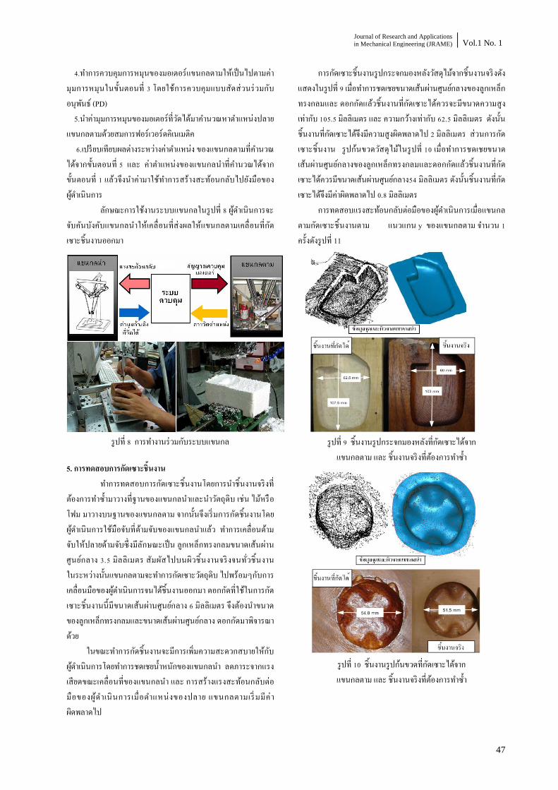
Journal of Research and Applications
in Mechanical Engineering (JRAME) Vol.1 No. 1
47
4.ท าการควบคมการหมนของมอเตอรแขนกลตามใหเปนไปตามคามมการหมนในขนตอนท 3 โดยใชการควบคมแบบสดสวนรวมกบอนพนธ (PD) 5.น าคามมการหมนของมอเตอรทวดไดมาค านวณหาต าแหนงปลายแขนกลตามดวยสมการฟอรเวอรดคเนเมตค 6.เปรยบเทยบผลตางระหวางคาต าแหนง ของแขนกลตามทค านวณไดจากขนตอนท 5 และ คาต าแหนงของแขนกลน าทค านวณไดจากขนตอนท 1 แลวจงน าคามาใชท าการสรางสะทอนกลบไปยงมอของผด าเนนการ ลกษณะการใชงานระบบแขนกลในรปท 8 ผด าเนนการจะจบคนบงคบแขนกลน าใหเคลอนทสงผลใหแขนกลตามเคลอนทกดเซาะชนงานออกมา
รปท 8 การท างานรวมกบระบบแขนกล
5. การทดสอบการกดเซาะชนงาน ท าการทดสอบการกดเซาะชนงานโดยการน าชนงานจรงท
ตองการท าซ ามาวางทฐานของแขนกลน าและน าวตถดบ เชน ไมหรอโฟม มาวางบนฐานของแขนกลตาม จากนนจงเรมการกดชนงานโดยผด าเนนการใชมอจบทดามจบของแขนกลน าแลว ท าการเคลอนดามจบใหปลายดามจบซงมลกษณะเปน ลกเหลกทรงกลมขนาดเสนผานศนยกลาง 3.5 มลลเมตร สมผสไปบนผวชนงานจรงจนทวชนงาน ในระหวางนนแขนกลตามจะท าการกดเซาะวตถดบ ไปพรอมๆกบการเคลอนมอของผด าเนนการจนไดชนงานออกมา ดอกกดทใชในการกดเซาะชนงานนมขนาดเสนผานศนยกลาง 6 มลลเมตร จงตองน าขนาดของลกเหลกทรงกลมและขนาดเสนผานศนยกลาง ดอกกดมาพจารณาดวย
ในขณะท าการกดชนงานจะมการเพมความสะดวกสบายใหกบผด าเนนการโดยท าการชดเชยน าหนกของแขนกลน า ลดภาระจากแรงเสยดขณะเคลอนทของแขนกลน า และ การสรางแรงสะทอนกลบตอมอของผ ด าเนนการเมอต าแหนงของปลาย แขนกลตามเรมมคาผดพลาดไป
การกดเซาะชนงานรปกระจกมองหลงวสดไมจากชนงานจรงดงแสดงในรปท 9 เมอท าการชดเชยขนาดเสนผานศนยกลางของลกเหลกทรงกลมและ ดอกกดแลวชนงานทกดเซาะไดควรจะมขนาดความสงเทากบ 105.5 มลลเมตร และ ความกวางเทากบ 62.5 มลลเมตร ดงนนชนงานทกดเซาะไดจงมความสงผดพลาดไป 2 มลลเมตร สวนการกดเซาะชนงาน รปกนขวดวสดไมในรปท 10 เมอท าการชดเชยขนาด เสนผานศนยกลางของลกเหลกทรงกลมและดอกกดแลวชนงานทกดเซาะไดควรมขนาดเสนผานศนยกลาง54 มลลเมตร ดงนนชนงานทกดเซาะไดจงมคาผดพลาดไป 0.8 มลลเมตร
การทดสอบแรงสะทอนกลบตอมอของผด าเนนการเมอแขนกลตามกดเซาะชนงานตาม แนวแกน y ของแขนกลตาม จ านวน 1 ครงดงรปท 11
รปท 9 ชนงานรปกระจกมองหลงทกดเซาะไดจาก
แขนกลตาม และ ชนงานจรงทตองการท าซ า
รปท 10 ชนงานรปกนขวดทกดเซาะไดจาก แขนกลตาม และ ชนงานจรงทตองการท าซ า
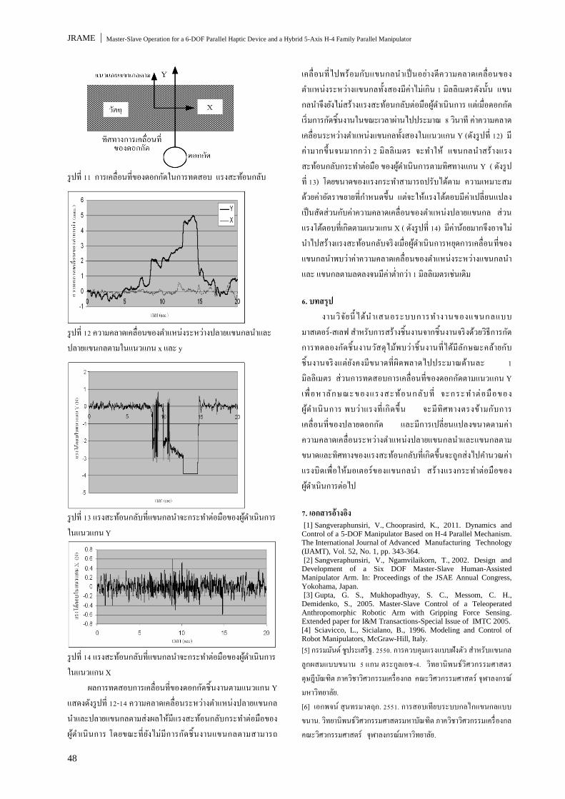
JRAME Master-Slave Operation for a 6-DOF Parallel Haptic Device and a Hybrid 5-Axis H-4 Family Parallel Manipulator
48
รปท 11 การเคลอนทของดอกกดในการทดสอบ แรงสะทอนกลบ
รปท 12 ความคลาดเคลอนของต าแหนงระหวางปลายแขนกลน าและปลายแขนกลตามในแนวแกน x และ y
รปท 13 แรงสะทอนกลบทแขนกลน าจะกระท าตอมอของผด าเนนการในแนวแกน Y
รปท 14 แรงสะทอนกลบทแขนกลน าจะกระท าตอมอของผด าเนนการในแนวแกน X
ผลการทดสอบการเคลอนทของดอกกดชนงานตามแนวแกน Y แสดงดงรปท 12-14 ความคลาดเคลอนระหวางต าแหนงปลายแขนกลน าและปลายแขนกลตามสงผลใหมแรงสะทอนกลบกระท าตอมอของผด าเนนการ โดยขณะทยงไมมการกดชนงานแขนกลตามสามารถ
เคลอนทไปพรอมกบแขนกลน าเปนอยางดความคลาดเคลอนของต าแหนงระหวางแขนกลทงสองมคาไมเกน 1 มลลเมตรดงนน แขนกลน าจงยงไมสรางแรงสะทอนกลบตอมอผด าเนนการ แตเมอดอกกดเรมการกดชนงานในขณะเวลาผานไปประมาณ 8 วนาท คาความคลาดเคลอนระหวางต าแหนงแขนกลทงสองในแนวแกน Y (ดงรปท 12) มคามากขนจนมากกวา 2 มลลเมตร จะท าให แขนกลน าสรางแรงสะทอนกลบกระท าตอมอ ของผด าเนนการตามทศทางแกน Y ( ดงรปท 13) โดยขนาดของแรงกระท าสามารถปรบไดตาม ความเหมาะสมดวยคาอตราขยายทก าหนดขน แตจะใหแรงโตตอบมคาเปลยนแปลง เปนสดสวนกบคาความคลาดเคลอนของต าแหนงปลายแขนกล สวนแรงโตตอบทเกดตามแนวแกน X ( ดงรปท 14) มคานอยมากจงอาจไมน าไปสรางแรงสะทอนกลบจรงเมอผด าเนนการหยดการเคลอนทของแขนกลน าพบวาคาความคลาดเคลอนของต าแหนงระหวางแขนกลน าและ แขนกลตามลดลงจนมคาต ากวา 1 มลลเมตรเชนเดม
6. บทสรป งานวจยนไดน าเสนอระบบการท างานของแขนกลแบบ
มาสเตอร-สเลฟ ส าหรบการสรางชนงานจากชนงานจรงดวยวธการกด การทดลองกดชนงานวสดไมพบวาชนงานทไดมลกษณะคลายกบชนงานจรงแตยงคงมขนาดทผดพลาดไปประมาณดานละ 1 มลลเมตร สวนการทดสอบการเคลอนทของดอกกดตามแนวแกน Y เ พอหาลกษณะของแรงสะทอนกลบ ท จะกระท าตอมอของผ ด าเนนการ พบวาแรงทเกดขน จะมทศทางตรงขามกบการเคลอนทของปลายดอกกด และมการเปลยนแปลงขนาดตามคาความคลาดเคลอนระหวางต าแหนงปลายแขนกลน าและแขนกลตาม ขนาดและทศทางของแรงสะทอนกลบทเกดขนจะถกสงไปค านวณคาแรงบดเพอใหมอเตอรของแขนกลน า สรางแรงกระท าตอมอของผด าเนนการตอไป
7. เอกสารอางอง [1] Sangveraphunsiri, V., Chooprasird, K., 2011. Dynamics and
Control of a 5-DOF Manipulator Based on H-4 Parallel Mechanism. The International Journal of Advanced Manufacturing Technology
(IJAMT), Vol. 52, No. 1, pp. 343-364.
[2] Sangveraphunsiri, V., Ngamvilaikorn, T., 2002. Design and Development of a Six DOF Master-Slave Human-Assisted
Manipulator Arm. In: Proceedings of the JSAE Annual Congress,
Yokohama, Japan. [3] Gupta, G. S., Mukhopadhyay, S. C., Messom, C. H.,
Demidenko, S., 2005. Master-Slave Control of a Teleoperated
Anthropomorphic Robotic Arm with Gripping Force Sensing. Extended paper for I&M Transactions-Special Issue of IMTC 2005.
[4] Sciavicco, L., Sicialano, B., 1996. Modeling and Control of
Robot Manipulators, McGraw-Hill, Italy.
[5] กรรมมนต ชประเสรฐ. 2550. การควบคมแรงแบบฝงตว ส าหรบแขนกลลกผสมแบบขนาน 5 แกน ตระกลเอช-4. วทยานพนธวศวกรรมศาสตร ดษฎบณฑต ภาควชาวศวกรรมเครองกล คณะวศวกรรมศาสตร จฬาลงกรณมหาวทยาลย. [6] เอกพจน สนทรมาตฤก. 2551. การสอบเทยบระบบกลไกแขนกลแบบขนาน. วทยานพนธวศวกรรมศาสตรมหาบณฑต ภาควชาวศวกรรมเครองกล คณะวศวกรรมศาสตร จฬาลงกรณมหาวทยาลย.

*ผตดตอ: E-mail: [email protected] โทรศพท, โทรสาร: 037 393 487
Vol. 1 No.1 TSME | Journal of Research and Applications in Mechanical Engineering
การวเคราะหความตานทานและรปแบบคลนของเรอแบบตวเรอค ดวยวธค านวณทางพลศาสตรของไหล
The Analysis of Resistance and Wave of Catamaran
Using Computational Fluid Dynamics
กตตภม ภมโคกรกษ1
, สตยา จนทรประภา1
และ อโณทย สขแสงพนมรง2,*
1กองออกแบบตอเรอ กรมแผนการชาง กรมอทหารเรอ แขวงศรราช เขตบางกอกนอย กรงเทพ ฯ 10700
2กองวชาวศวกรรมเครองกล สวนการศกษา โรงเรยนนายรอยพระจลจอมเกลา อ.เมอง จ.นครนายก 26001
บทคดยอ
งานวจยนเปนการประยกตใชวธการค านวณทางพลศาสตรของไหล (Computational Fluid Dynamics) วธ Finite Volume Method จ าลองการไหลผานเรอแบบตวเรอค (Catamaran) เพอวเคราะหความตานทานและรปแบบคลนทเกดจากเรอในยานการใชงานส าหรบเรอโดยสารในแมน า ผลการวจยพบวาเมอเลขฟรดเชงความยาวแนวน า ( Fn ) มคา 0.5 – 0.7 สมประสทธความตานทานเรอ (
TC ) มคาลดลงและสมประสทธความ
ตานทานเชงคลน ( WC ) มคาลดลง ขณะทสมประสทธความตานทานความหนด (VC ) มคาคงท เมอเลขฟรดเชงความลกของน า ( hFn ) เทากบ
0.6 – 0.7 พบวาคลนมความสงเพมขนและเดนทางไดไกลขนเมอความลกของน าทลดลง งานวจยนสามารถใชเปนแนวทางในการออกแบบเรอแบบตวเรอคเบองตนเพอใหไดเรอทประหยดพลงงานและลดผลกระทบดานสงแวดลอมอนเกดจากคลนทเกดจากเรอ อยางไรกตามในอนาคตควรจะไดมการศกษาการแบงกรดทเหมาะสมตลอดจนแบบจ าลองทางคณตศาสตรทสงขนเพอใหไดผลใกลเคยงกบความเปนจรงมากทสดตอไป
ค าหลก: วธค านวณทางพลศาสตรของไหล, เรอแบบตวเรอค, ความตานทานเรอ, รปแบบคลน, เรอโดยสาร
Abstract
This study was performed to analyse the total resistance and wave profile of a catamaran using Computational Fluid
Dynamics - the Finite Volume Method. The work was conducted within the operating conditions of the waterbus service in the
Chaophraya River, Bangkok. The total resistance was analysed at different operating speeds with the corresponding waterline
Froude number ( Fn ) equal to 0.5 – 0.7. Within the study range, the calculated total resistance coefficient ( ) and wave-
making resistance coefficient ( ) were found to decrease as the decreased. While the viscous resistance coefficient
( ) was almost unchanged. The waves generated when the catamaran sailed through calm water were then analysed at the
depth Froude number ( hFn ) between 0.6 - 0.7 corresponding to the maximum and minimum route depths. It was found that the
calculated wave profiles increased as the depth decreased. The waves generated in shallow water also travelled in longer
distance than those generated in deeper water. The study has shown that the method developed here could be practically applied
in the preliminary design of actual catamarans where energy-saving and environment friendliness are the key design. However, a
further study with finer meshing and more advanced mathematical models should be conducted in order to achieve more
accurate results.
Keywords: Computational Fluid Dynamics, catamaran, total resistance, wave profile, waterbus
1. บทน า เรอแบบตวเรอค (Catamaran) เปนเรอประเภททมตวเรอ 2 ล า เชอมตอกนดวยโครงสรางดาดฟาเรอดงรปท 1 เมอเปรยบเทยบกบเรอแบบตวเรอเดยว (Monohull) ทระวางขบน าเทากนแลว เรอแบบตวเรอคสามารถออกแบบรปทรงตวเรอ (Hull form) ใหมความเพรยวได
มากกวา สงผลใหความตานทานของเรอลดลงโดยไมท าใหการทรงตวของเรอเสยไป เรอประเภทนมความเหมาะสมในการน ามาใชเปนเรอโดยสารลดคลนและประหยดพลงงาน โดยเฉพาะเรอโดยสารในแมน า เชน แมน าเจาพระยา ซงปจจบนประสบปญหาการพงทลายของพนทรมฝงแมน าเนองจากคลนทเกดจากเรอ [1]
TC
WC Fn
VC

JRAME The Analysis of Resistance and Wave of Catamaran Using Computational Fluid Dynamics
50
รปท 1 เรอแบบตวเรอค (Catamaran)
การศกษาองคประกอบความตานทานของเรอแบบตวเรอค โดยการทดลองลากเรอจ าลองในถงลากเรอ (Towing tank test) ซงเปนวธทใหคาใกลเคยงความเปนจรงมากทสด ไดมการวจยอยางแพรหลาย เชน Insel และ Molland [2] พบวาความตานทานความหนด (Viscous resistance) มคาขนอยกบความเพรยวของเรอแตไมขนกบความเรวและระยะหางระหวางตวเรอค ขณะท Couser และคณะ [3] แสดงใหเหนวาส าหรบเรอแบบตวเรอคประเภทความเรวสงทมตวเรอเพรยว ความตานทานความหนดมคามากกวาความตานทานเชงคลน (Wave-making resistance) ตอมา Utama และ Molland [4] พบวาอทธพลของการแทรกสอดของคลนระหวางตวเรอคมผลตอความตานทานความหนดเพยงเลกนอย
นอกเหนอจากการวธทดลองขางตนแลว การค านวณทางพลศาสตรของไหล (Computational Fluid Dynamics หรอ CFD) กเปนอกวธหนงทนยมน ามาใชจ าลองการไหลผานเรอ เนองจากมคาใชจายและใช เวลานอย ประกอบกบความกาวหนาทาง เทคโนโลยคอมพวเตอรท าใหการค านวณและการแสดงผล มประสทธภาพมากขน อาทเชน Armstrong [5] ไดใชวธ CFD แบบปรมาตรจ ากด (Finite Volume Method หรอ FVM) จ าลองการไหลผานเรอแบบตวเรอคประเภทความเรวสง พบวาการกระจายของความดนรอบตวเรอสอดคลองกบผลการทดลอง ขณะท Thornhill และคณะ [6] ไดใชวธ FVM วเคราะหความตานทานของเรอประเภท Planing craft ซงพบวา แมวาการวเคราะหจะเปนการค านวณในสภาวะคงตว(Steady flow) แตเพอใหไดผลสอดคลองกบความเปนจรงจ าเปนจะตองใชวธค านวณแบบแปรผนตามเวลา(Transient) ทงนงานวจยทงสองเปนการจ าลองการไหลแบบปนปวนโดยไมรวมการเปลยนแปลงทผวน า ส าหรบการวเคราะหรปแบบคลนดวยวธ CFD นน ไดมงานวจยทน าแบบจ าลองปรมาตรของไหล (Volume Of Fluid หรอ VOF) มาใชตดตามการเปลยนแปลงทผวน า เชน การศกษาการไหลแบบไมมความหนดรอบตวเรอสนคาในเขตน าตนของ Tabaczek [7]
จากทกลาวมาขางตน งานวจยนจงไดน าวธการค านวณทาง
พลศาสตรของไหลแบบปรมาตรจ ากด ทพจารณาการไหลแบบมความหนดประกอบกบมการเปลยนแปลงทผวน า มาวเคราะหความตานทานและรปแบบคลนทเกดจากเรอแบบตวเรอค เพอเปนแนวทางในการออกแบบเบองตน (Preliminary design) ส าหรบเรอโดยสารแบบตวเรอคทเหมาะส าหรบการใชงานในแมน า ดวยเงอนไขของความเรวสงสดไมเกน 20 กโลเมตร/ชวโมง ทความลกต าสดและสงสดเทากบ 6.5 เมตร และ 8.5 เมตร ตามล าดบ
2. ทฤษฎทเกยวของ 2.1 ความตานทานเรอ
ความตานทานรวมของเรอ (Total ship resistance หรอ ) สามารถค านวณไดจาก
(1)
โดยท คอคาสมประสทธความตานทานเรอรวม (Total ship resistance coefficient) ในทางปฏบตจากทประชม International Towing Tank Conference [8] สามารถแบงองคประกอบหลกของ
ออกเปน
(2)
โดยท คอคาสมประสทธความตานทานความหนด (Viscous
resistance coefficient) และ คอคา สมประสทธความตานทานเชงคลน (Wave-making resistance coefficient) ทงนความตานทานเชงคลนมคาขนอยกบเลขฟรด (Froude number หรอ Fn ) ซงหาคาไดจาก
VFn
gL (3)
TR
21
2T TR AV C
TC
TC
T V WC C C
VC
WC
หวเรอ ทายเรอ
แนวน า
ดาดฟาเรอ
ตวเรอค
พนทองน า
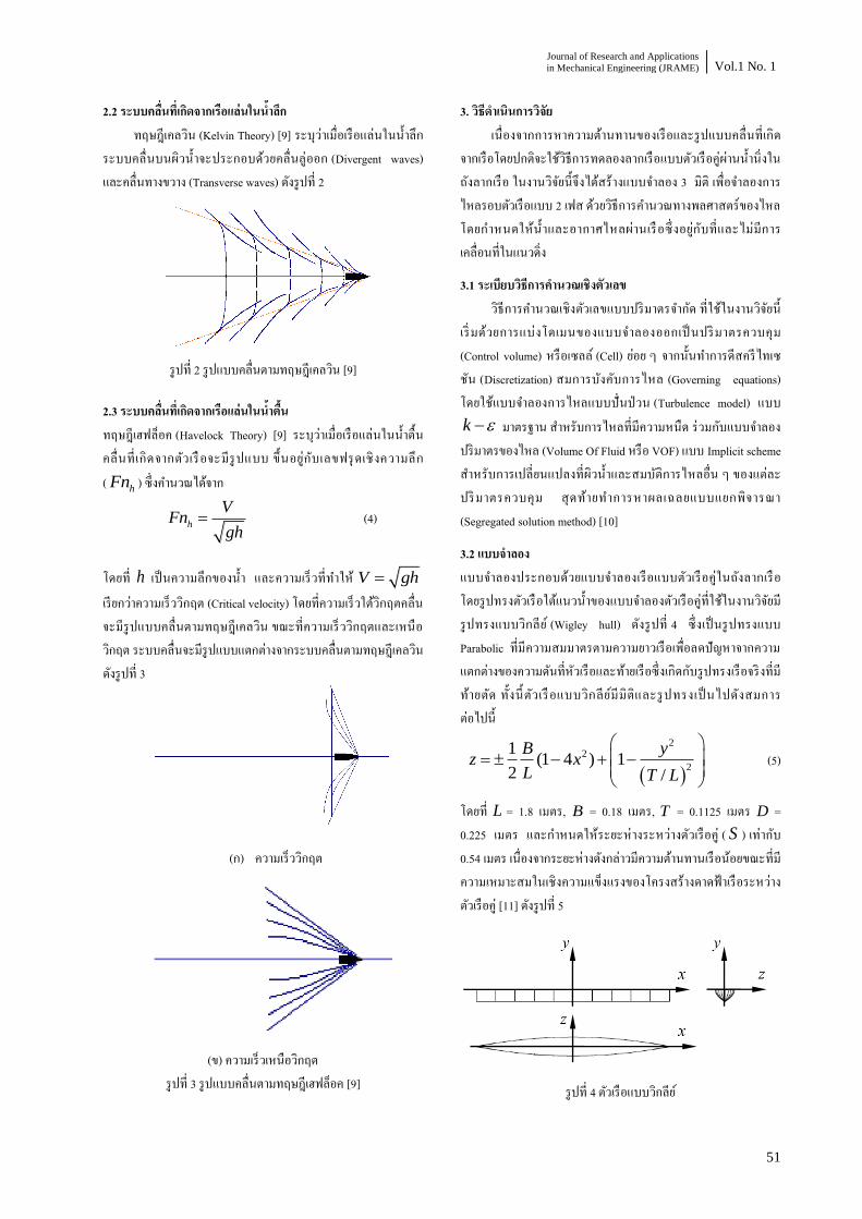
Journal of Research and Applications
in Mechanical Engineering (JRAME) Vol.1 No. 1
51
2.2 ระบบคลนทเกดจากเรอแลนในน าลก ทฤษฎเคลวน (Kelvin Theory) [9] ระบวาเมอเรอแลนในน าลก
ระบบคลนบนผวน าจะประกอบดวยคลนลออก (Divergent waves) และคลนทางขวาง (Transverse waves) ดงรปท 2
รปท 2 รปแบบคลนตามทฤษฎเคลวน [9]
2.3 ระบบคลนทเกดจากเรอแลนในน าตน ทฤษฎเฮฟลอค (Havelock Theory) [9] ระบวาเมอเรอแลนในน าตน คลนทเกดจากตวเรอจะมรปแบบ ขนอยกบเลขฟรดเชงความลก ( ) ซงค านวณไดจาก
(4)
โดยท h เปนความลกของน า และความเรวทท าให V gh
เรยกวาความเรววกฤต (Critical velocity) โดยทความเรวใตวกฤตคลนจะมรปแบบคลนตามทฤษฎเคลวน ขณะทความเรววกฤตและเหนอวกฤต ระบบคลนจะมรปแบบแตกตางจากระบบคลนตามทฤษฎเคลวน ดงรปท 3
(ก) ความเรววกฤต
(ข) ความเรวเหนอวกฤต รปท 3 รปแบบคลนตามทฤษฎเฮฟลอค [9]
3. วธด าเนนการวจย เนองจากการหาความตานทานของเรอและรปแบบคลนทเกด
จากเรอโดยปกตจะใชวธการทดลองลากเรอแบบตวเรอคผานน านงในถงลากเรอ ในงานวจยนจงไดสรางแบบจ าลอง 3 มต เพอจ าลองการไหลรอบตวเรอแบบ 2 เฟส ดวยวธการค านวณทางพลศาสตรของไหล โดยก าหนดใหน าและอากาศไหลผานเรอซงอยกบทและไมมการเคลอนทในแนวดง
3.1 ระเบยบวธการค านวณเชงตวเลข วธการค านวณเชงตวเลขแบบปรมาตรจ ากด ทใชในงานวจยน
เรมดวยการแบงโดเมนของแบบจ าลองออกเปนปรมาตรควบคม (Control volume) หรอเซลล (Cell) ยอย ๆ จากนนท าการดสครไทเซชน (Discretization) สมการบงคบการไหล (Governing equations) โดยใชแบบจ าลองการไหลแบบปนปวน (Turbulence model) แบบ
มาตรฐาน ส าหรบการไหลทมความหนด รวมกบแบบจ าลองปรมาตรของไหล (Volume Of Fluid หรอ VOF) แบบ Implicit scheme ส าหรบการเปลยนแปลงทผวน าและสมบตการไหลอน ๆ ของแตละปรมาตรควบคม สดทายท าการหาผลเฉลยแบบแยกพจารณา (Segregated solution method) [10]
3.2 แบบจ าลอง แบบจ าลองประกอบดวยแบบจ าลองเรอแบบตวเรอคในถงลากเรอ โดยรปทรงตวเรอใตแนวน าของแบบจ าลองตวเรอคทใชในงานวจยมรปทรงแบบวกลย (Wigley hull) ดงรปท 4 ซงเปนรปทรงแบบ Parabolic ทมความสมมาตรตามความยาวเรอเพอลดปญหาจากความแตกตางของความดนทหวเรอและทายเรอซงเกดกบรปทรงเรอจรงทมทายตด ท งนตวเรอแบบวกลยมมตและรปทรงเปนไปดงสมการตอไปน
(5)
โดยท = 1.8 เมตร, B = 0.18 เมตร, T = 0.1125 เมตร D = 0.225 เมตร และก าหนดใหระยะหางระหวางตวเรอค ( S ) เทากบ 0.54 เมตร เนองจากระยะหางดงกลาวมความตานทานเรอนอยขณะทมความเหมาะสมในเชงความแขงแรงของโครงสรางดาดฟาเรอระหวางตวเรอค [11] ดงรปท 5
รปท 4 ตวเรอแบบวกลย
hFn
h
VFn
gh
k
22
2
1(1 4 ) 1
2 /
B yz x
L T L
L

JRAME The Analysis of Resistance and Wave of Catamaran Using Computational Fluid Dynamics
52
รปท 5 แบบจ าลองตวเรอค
แบบจ าลองถงลากเรอมขนาดและรปทรงสอดคลองกบงานวจยของ Insel และ Molland [2] โดยเปนแบบจ าลองเฉพาะตวเรอคซงรวมทงตวเรอเหนอและใตแนวน า แตไมรวมโครงสรางดาดฟาเรอและเกงเรอ (Superstructure) เพอประโยชนในการตรวจสอบโปรแกรม ยกเวนสวนบรรยากาศและความยาวของถงเนองจากขอจ ากดดานการแบง กรดของโดเมน โดยมขนาดเปนดงรปท 6
การแบ งก รดส าห รบงาน วจย น ใ ช รปทรงหกหน า (Hexahedron) เชงโครงสรางปกต (Structured grid) แบบ Map scheme เพอหลกเลยงการแบงกรดครอมแนวน าซงจะท าใหเกดความผดพลาดในการก าหนดคาเรมตนของสดสวนปรมาตร (Volume fraction) ในแบบจ าลอง VOF โดยปรมาตรควบคมมความละเอยดมากทสดบรเวณผวตวเรอและผวน า จากนนการแบงกรดจะหยาบขนเมอหางออกไป ดงรปท 7 โดยมจ านวนปรมาตรควบคมทงสน 588,000 เซลล
รปท 6 โดเมนแบบจ าลอง (หนวยเปนเมตร)
รปท 7 การแบงกรด
3.3 สมการพนฐาน ก าหนดใหการไหลรอบตวเรอเปนการไหลแบบอดตวไมได ทไมมการเปลยนแปลงของอณหภม และมสมบตการไหลเทากนทกทศทาง ดวยวธการ Reynolds Average ส าหรบการไหลแบบปนปวน ก าหนดใหคณสมบตการไหล ณ เวลาใด ๆ ( ) ประกอบดวย สวนคาเฉลย ( ) และสวนความปนปวน ( ) ดงสมการ
(6)
ก าหนดให u เ ปน เ วก เตอรความเ รว ทไหลในพกดฉาก
( ˆˆ ˆui vj wk u ) โดยท u U + u สมการควบคมการไหลส าหรบงานวจยนประกอบดวย
สมการความตอเนอง (Continuity equation)
. 0U (7)
สมการ Reynolds-Averaged Navier-Stokes equation (RANS) + Eddy viscosity hypothesis
1
. . .
m
U UU U StPt
โดยท 2
t
kC และ mS คอ source term
สมการ k ส าหรบการจ าลองการไหลแบบปนปวน (เทอม t )
. . 2U
tt ij ij
k
k k k E Et
2
1 2. . 2U
tt ij ijC E E C
t k k
คาคงท
10.09, 1.00, 1.00, 1.44 kC C
และ 2 1.92 C [10]
3.4 แบบจ าลองปรมาตรของไหล VOF เมอก าหนดใหอากาศเปนเฟสปฐมภม (Primary phase) และน าเปนเฟสทตยภม (Secondary phase) เราสามารถค านวณสดสวนปรมาตรของน า ( water ) และอากาศ ( air ) ในปรมาตรควบคมใด ๆ ไดจากสมการ ตอไปน
. 0waterwater
t
u
(8)
(9)
(10)
(11)
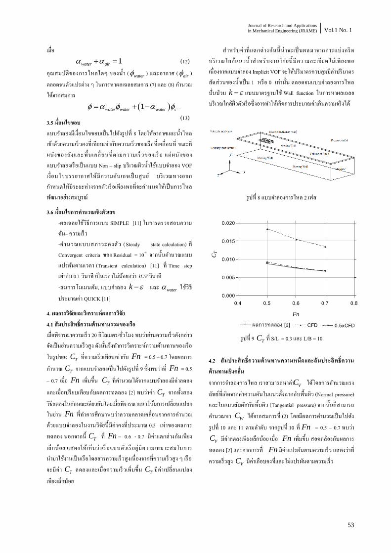
Journal of Research and Applications
in Mechanical Engineering (JRAME) Vol.1 No. 1
53
เมอ 1 water air
คณสมบตของการไหลใดๆ ของน า ( water ) และอากาศ (air )
ตลอดจนตวแปรตาง ๆ ในการหาผลเฉลยสมการ (7) และ (8) ค านวณไดจากสมการ 1water water water air
3.5 เงอนไขขอบ แบบจ าลองมเงอนไขขอบเปนไปดงรปท 8 โดยใหอากาศและน าไหลเขาดวยความเรวคงทเทยบเทากบความเรวของเรอทเคลอนท ขณะทผนงของถงและพนเคลอนทตามความเรวของเรอ แตผนงของแบบจ าลองเรอเปนแบบ Non – slip บรเวณผวน าใชแบบจ าลอง VOF เ งอนไขบรรยากาศใหมความดนเกจเปนศนย บรเวณทางออกก าหนดใหมระยะหางจากตวเรอเพยงพอทจะก าหนดใหเปนการไหลพฒนาอยางสมบรณ
3.6 เงอนไขการค านวณเชงตวเลข -ผลเฉลยใชวธการแบบ SIMPLE [11] ในการตรวจสอบความดน– ความเรว -ค านวณแบบสภาวะคงตว (Steady state calculation) ท Convergent criteria ของ Residual = 10-4 จากนนค านวณแบบแปรผนตามเวลา (Transient calculation) [11] ท Time step เทากบ 0.1 วนาท เปนเวลาไมนอยกวา 3L/V วนาท -สมการโมเมนตม, แบบจ าลอง k และ water ใชวธประมาณคา QUICK [11]
4. ผลการวจยและวเคราะหผลการวจย 4.1 สมประสทธความตานทานรวมของเรอ เมอพจารณาความเรว 20 กโลเมตร/ชวโมง พบวายานความเรวดงกลาวจดเปนยานความเรวสง ดงนนจงท าการวเคราะหความตานทานของเรอในรปของ TC ทความเรวเทยบเทากบ = 0.5 – 0.7 โดยผลการ
ค านวณ TC จากแบบจ าลองเปนไปดงรปท 9 ซงพบวาท Fn = 0.5
– 0.7 เมอ Fn เพมขน ทค านวณไดจากแบบจ าลองมคาลดลง
และเมอเปรยบเทยบกบผลการทดลอง [2] พบวาคา TC จากทงสองวธลดลงในลกษณะเดยวกนโดยเมอพจารณาแนวโนมการเปลยนแปลงในยาน Fn ทท าการศกษาพบวาความคลาดเคลอนจากการค านวณดวยแบบจ าลองในงานวจยนมคาคงทประมาณ 0.5 เทาของผลการทดลอง นอกจากน ท Fn = 0.6 - 0.7 มคาแตกตางกนเพยงเลกนอย แสดงใหเหนวาเรอแบบตวเรอคมความเหมาะสมในการน ามาใชงานเปนเรอโดยสารความเรวสงเนองจากทความเรวสง ๆ เรอจะมคา ลดลงและเมอความเรวเพมขน มคาเปลยนแปลงเพยงเลกนอย
ส าหรบคาทแตกตางกนนนาจะเปนผลมาจากการแบงกรด บรเวณใกลแนวน าส าหรบงานวจยนมความละเอยดไมเพยงพอเนองจากแบบจ าลอง Implicit VOF จะใหปรมาตรควบคมมคาปรมาตรสดสวนของน าเปน 1 หรอ 0 เทานน ตลอดจนแบบจ าลองการไหลปนปวน k แบบมาตรฐานใช Wall function ในการหาผลเฉลยบรเวณใกลผวตวเรอซงอาจท าใหเกดการประมาณคาเกนความจรงได
รปท 8 แบบจ าลองการไหล 2 เฟส
0.4 0.5 0.6 0.7 0.80.000
0.005
0.010
0.015
0.020
ผลการทดลอง [2] CFD 0.5xCFD
Fn
CT
รปท 9 TC ท S/L = 0.3 และ L/B = 10 4.2 สมประสทธความตานทานความหนดและสมประสทธความตานทานเชงคลน
จากการจ าลองการไหล เราสามารถหาคา ไดโดยการค านวณแรงลพธทเกดจากคาความดนในแนวตงฉากกบพนผว (Normal pressure) และในแนวสมผสกบพนผว (Tangential pressure) จากนนกสามารถค านวณหา ไดจากสมการท (2) โดยมผลการค านวณเปนไปดงรปท 10 และ 11 ตามล าดบ จากรปท 10 ท = 0.5 – 0.7 พบวา
มคาลดลงเพยงเลกนอย เมอ เพมขน สอดคลองกบผลการทดลอง [2] และจากการท มคาแปรผนตามความเรว แสดงวาทความเรวสง VC มคาเกอบคงทและไมแปรผนตามความเรว
Fn
TC
TC
TC TC
VC
WC
Fn
VC Fn
Fn
(12)
(13)
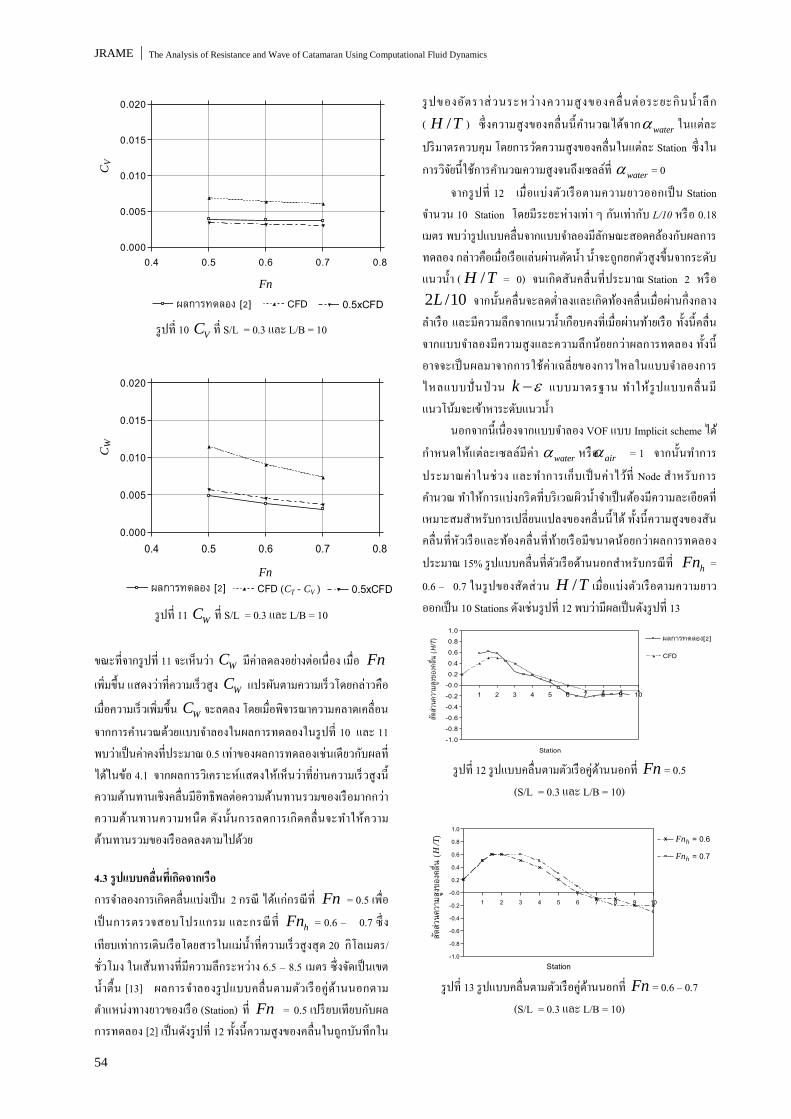
JRAME The Analysis of Resistance and Wave of Catamaran Using Computational Fluid Dynamics
54
0.4 0.5 0.6 0.7 0.80.000
0.005
0.010
0.015
0.020
ผลการทดลอง [2] CFD 0.5xCFDFn
CV
รปท 10 VC ท S/L = 0.3 และ L/B = 10
0.4 0.5 0.6 0.7 0.80.000
0.005
0.010
0.015
0.020
ผลการทดลอง [2] CFD (CT - CV ) 0.5xCFDFn
CW
รปท 11 WC ท S/L = 0.3 และ L/B = 10 ขณะทจากรปท 11 จะเหนวา มคาลดลงอยางตอเนอง เมอ
เพมขน แสดงวาทความเรวสง แปรผนตามความเรวโดยกลาวคอ
เมอความเรวเพมขน จะลดลง โดยเมอพจารณาความคลาดเคลอนจากการค านวณดวยแบบจ าลองในผลการทดลองในรปท 10 และ 11 พบวาเปนคาคงทประมาณ 0.5 เทาของผลการทดลองเชนเดยวกบผลทไดในขอ 4.1 จากผลการวเคราะหแสดงใหเหนวาทยานความเรวสงนความตานทานเชงคลนมอทธพลตอความตานทานรวมของเรอมากกวาความตานทานความหนด ดงนนการลดการเกดคลนจะท าใหความตานทานรวมของเรอลดลงตามไปดวย
4.3 รปแบบคลนทเกดจากเรอ การจ าลองการเกดคลนแบงเปน 2 กรณ ไดแกกรณท = 0.5 เพอเปนการตรวจสอบโปรแกรม และกรณท hFn = 0.6 – 0.7 ซงเทยบเทาการเดนเรอโดยสารในแมน าทความเรวสงสด 20 กโลเมตร/ชวโมง ในเสนทางทมความลกระหวาง 6.5 – 8.5 เมตร ซงจดเปนเขตน าตน [13] ผลการจ าลองรปแบบคลนตามตวเรอคดานนอกตามต าแหนงทางยาวของเรอ (Station) ท = 0.5 เปรยบเทยบกบผลการทดลอง [2] เปนดงรปท 12 ทงนความสงของคลนในถกบนทกใน
รปของอตราสวนระหวางความสงของคลนตอระยะกนน าลก ( ) ซงความสงของคลนนค านวณไดจาก
water ในแตละปรมาตรควบคม โดยการวดความสงของคลนในแตละ Station ซงในการวจยนใชการค านวณความสงจนถงเซลลท
water = 0 จากรปท 12 เมอแบงตวเรอตามความยาวออกเปน Station
จ านวน 10 Station โดยมระยะหางเทา ๆ กนเทากบ L/10 หรอ 0.18 เมตร พบวารปแบบคลนจากแบบจ าลองมลกษณะสอดคลองกบผลการทดลอง กลาวคอเมอเรอแลนผานตดน า น าจะถกยกตวสงขนจากระดบแนวน า ( /H T = 0) จนเกดสนคลนทประมาณ Station 2 หรอ 2 /10L จากนนคลนจะลดต าลงและเกดทองคลนเมอผานกงกลางล าเรอ และมความลกจากแนวน าเกอบคงทเมอผานทายเรอ ทงนคลนจากแบบจ าลองมความสงและความลกนอยกวาผลการทดลอง ทงนอาจจะเปนผลมาจากการใชคาเฉลยของการไหลในแบบจ าลองการไหลแบบปนปวน k แบบมาตรฐาน ท าให รปแบบคลนมแนวโนมจะเขาหาระดบแนวน า
นอกจากนเนองจากแบบจ าลอง VOF แบบ Implicit scheme ไดก าหนดใหแตละเซลลมคา
water หรอ = 1 จากนนท าการประมาณคาในชวง และท าการเกบเปนคาไวท Node ส าหรบการค านวณ ท าใหการแบงกรดทบรเวณผวน าจ าเปนตองมความละเอยดทเหมาะสมส าหรบการเปลยนแปลงของคลนนได ทงนความสงของสนคลนทหวเรอและทองคลนททายเรอมขนาดนอยกวาผลการทดลองประมาณ 15% รปแบบคลนทตวเรอดานนอกส าหรบกรณท
hFn = 0.6 – 0.7 ในรปของสดสวน /H T เมอแบงตวเรอตามความยาวออกเปน 10 Stations ดงเชนรปท 12 พบวามผลเปนดงรปท 13
1 2 3 4 5 6 7 8 9 10
-1.0-0.8-0.6-0.4-0.2-0.00.20.40.60.81.0
ผลการทดลอง[2]
CFD
Station
สดสว
นควา
มสงข
องคล
น (H/T)
รปท 12 รปแบบคลนตามตวเรอคดานนอกท Fn = 0.5 (S/L = 0.3 และ L/B = 10)
1 2 3 4 5 6 7 8 9 10
-1.0
-0.8
-0.6
-0.4
-0.2
-0.0
0.2
0.4
0.6
0.8
1.0Fnh = 0.6
Fnh = 0.7
Station
สดสว
นควา
มสงข
องคล
น (H
/T)
รปท 13 รปแบบคลนตามตวเรอคดานนอกท Fn = 0.6 – 0.7 (S/L = 0.3 และ L/B = 10)
WC Fn
WC
WC
Fn
Fn
/H T
air
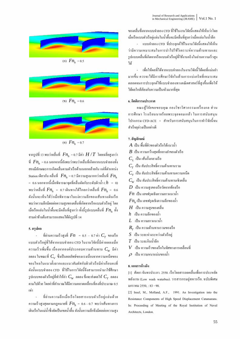
Journal of Research and Applications
in Mechanical Engineering (JRAME) Vol.1 No. 1
55
(ก) = 0.5
(ข) = 0.6
(ค) = 0.7
จากรปท 13 พบวาคลนท = 0.7 มคา /H T โดยเฉลยสงกวา
ท = 0.6 นอกจากนยงพบวาพบวาคลนทเกดจากแบบจ าลองทงสองมลกษณะการเกดคลนตามตวเรอดานนอกคลายกน แตทต าแหนง Station เดยวกน คลนท = 0.7 มความสงมากกวาคลนท
hFn = 0.6 นอกจากนเมอพจารณาจดทคลนตดกบระดบผวน า ( h = 0) พบวาคลนท = 0.7 เดนทางไดไกลกวาคลนท hFn = 0.6 ดงน นจะเหนไดวาเมอพจารณาในแงความลกของเสนทางเดนเรอ พบวาความลกมผลตอความสงของคลนทเกดจากเรอแบบตวเรอค โดยเมอเรอแลนในน าตนจะมคลนทสงกวา ทงนรปแบบคลนท hFn ทงสามคาขางตนสามารถแสดงไดดงรปท 14
5. สรปผล
- ทยานความเรวสงท = 0.5 – 0.7 คา TC ของเรอแบบตวเรอคทไดจากแบบจ าลอง CFD ในงานวจยนมคาลดลงเมอความเรวเพมขน เนองจากองคประกอบความตานทาน WC มคา
ลดลง ในขณะท VC ซงเปนผลลพธของแรงเนองจากความหนดของของไหลในแนวตงฉากและแนวสมผสกบผวตวเรอมคาเกอบคงท ดงนนแบบจ าลอง CFD ทใชในการวจยนจงสามารถน ามาใชศกษารปแบบของตวเรอคทท าใหคา WC ลดลง ซงจะสงผลให TC ลดลงตามไปดวย โดยคาทค านวณไดมความคลาดเคลอนทคงทประมาณ 0.5 เทา
- ทยานความลกเ มอเรอโดยสารแบบตวเ รอคแลนดวยความเรวสงสดตามกฎหมายท hFn = 0.6 – 0.7 พบวาเสนทางการเดนเรอในแมน าซงจดเปนเขตน าตน ดงนนความลกจงมผลตอความสง
ของคลนซงจากแบบจ าลอง CFD ทใชในงานวจยนแสดงใหเหนวาโดยเมอเรอแบบตวเรอคแลนในน าตนจะมคลนทสงกวาเมอแลนในน าลก
- แบบจ าลอง CFD ทประยกตใชในงานวจยนแสดงใหเหนวามความเหมาะสมในการน าไปใชวเคราะหความตานทานและรปแบบคลนทเกดจากเรอแบบตวเรอคทใชงานจรงในยานความเรวสงได
- เพอใหผลทไดจากแบบจ าลองในงานวจยนไดผลทแมนย ามากขน ควรจะไดมการศกษาวจยในดานการแบงกรดทเหมาะสมตลอดจนการประยกตใชแบบจ าลองทางคณตศาสตรทสงขนเพอใหไดผลใกลเคยงกบความเปนจรงมากทสด
6. กตตกรรมประกาศ คณะผวจยขอขอบคณ กองวชาวศวกรรมเครองกล สวน
การศกษา โรงเรยนนายรอยพระจลจอมเกลา ในการสนบสนนโปรแกรม CFD-ACE + ส าหรบการสนบสนนในการท าวจยนจนส าเรจลลวงเปนอยางด
7. สญลกษณ A เปน พนทผวของตวเรอใตแนวน า B เปน ความกวางสดทกลางล าของตวเรอ
LC เปน เสนกงกลางเรอ
เปน สมประสทธความตานทานรวม
VC เปน สมประสทธความตานทานความหนด
เปน สมประสทธความตานทานเชงคลน D เปน ความสงของเรอวดจากทองเรอ Fn เปน เลขฟรดเชงความยาวแนวน า
hFn เปน เลขฟรดเชงความลกของน า H เปน ความสงของคลน h เปน ความลกของน า
เปน ความยาวแนวน า
TR เปน ความตานทานรวมของเรอ S เปน ระยะหางระหวางตวเรอค T เปน ระยะกนน าลก V เปน ความเรวของเรอในทศทางการเคลอนท เปน ความหนาแนนของน า
8. เอกสารอางอง [1] สตยา จนทรประภา. 2550. เรอโดยสารลดคลนเพอการประหยดพลงงาน (Low wash waterbus). วารสารกรมอทหารเรอ. ฉบบพเศษ มกราคม 2550, : 83 - 90. [2] Insel, M., Molland, A.F., 1991. An Investigation into the Resistance Components of High Speed Displacement Catamarans. In: Proceeding of Meeting of the Royal Institution of Naval Architects, London.
hFn
hFn
hFn
hFn
hFn
hFn
hFn
Fn
TC
WC
L

JRAME The Analysis of Resistance and Wave of Catamaran Using Computational Fluid Dynamics
56
[3] Couser, P.R., et, al., 1997. Calm Water Powering Predictions for High-speed Catamarans. Fast, Vol. 97. [4] Utama, I.K.A.P., Molland, A.F., 2001. Experimental and Numerical Investigations into Catamaran Viscous Resistance. In: Proceedings of the Sixth International Conference on Fast Sea Transportation. Southampton University, England, pp. 295-306. [5] Armstrong, N., 1995. An Investigation into the Form Factor of High Speed Light Craft. In: Proceedings of the First AMECRC Postgraduate Student Conference, Australia. [6] Thornhill, E., et, al. 2003. Planing Hull Performance Evaluation Using a General Purpose CFD Code. In: Proceedings of 24th Symposium on Naval Hydrodynamics. [7] Tabaczek, T., 2008. Computation of Flow around Inland Waterway Vessel in Shallow Water. Archives of Civil and Mechanical Engineering, Vol. VIII, pp. 97 – 105. [8] International Towing Tank Conference. 1957. Skin Friction and Turbulence Simulation. In: Proceedings of the 8th ITTC, Madrid, Spain. Canal de Experiencias Hidrodinamics, El Pardo, Madrid, Spain. [9] Van Manen, J.D., Van Oossanen, P., 1988. Chapter V Resistance. Principles of Naval Architecture, Vol. III, Lewis, EV, editor. 1st printing, The Society of Naval Architects and Marine Engineers, USA, pp. 1 – 125. [10] Versteeg, H.K., Malalasekera, W. 1995. An Introduction to Computational Fluid Dynamics: The Finite Volume Method. 1st edition. Longman Group Ltd, England. [11] กตตภม ภมโคกรกษ และคณะ. 2553. การศกษาผลกระทบของระยะหางและความเพรยวของเรอแบบตวเรอคตอความตานทานเรอดวยวธค านวณทางพลศาสตรของไหล. การประชมสมมนาทางวชาการ มหาวทยาลยเทคโนโลยราชมงคลภาคตะวนออก ครงท 3. พทยา จ.ชลบร. [12] Patankar, S. 1980. Numerical Heat Transfer and Fluid Flow. 1st edition, Hemisphere, Washington D.C., USA. [13] Leer-Anderson, M., et al., 2000. Wash Waves – Problems and Solutions, In: Proceedings of the Society of Naval Architects and Marine Engineers Annual Meeting.

*ผตดตอ: E-mail: [email protected] โทรศพท: 02-5643001-9 ตอ 3144, โทรสาร: ตอ 3049
Vol. 1 No.1 TSME | Journal of Research and Applications in Mechanical Engineering
ผลของการเรยงขวอเลกโตรดทมตอการอบแหงดวยลมรอนรวมกบสนามไฟฟา Effects of Electrode Arrangement on the combined Hot-Air Flow
and Electric Field Drying
ธชพงศ กรวชรนทร ไชยณรงค จกรธรานนท* และ ผดงศกด รตนเดโช
ภาควชาวศวกรรมเครองกล คณะวศวกรรมศาสตร มหาวทยาลยธรรมศาสตร ศนยรงสต 99 หม 18 ต าบลคลองหนง อ าเภอคลองหลวง จงหวดปทมธาน 12120
บทคดยอ
งานวจยนศกษาอทธพลของการจดเรยงแทงอเลกโตรดทมตอการเพมประสทธภาพการอบแหงในวสดพรนโดยใชลมรอนรวมกบสนามไฟฟา โดยตวแปรทท าการศกษา คอ จ านวนขวอเลกโตรด (n = 1, 3, และ 4 ขว) และ ระยะระหวางอเลกโตรดและกราวด (L = 2 - 8 cm) แรงดนไฟฟาทใชเพอท าใหเกดโคโรนาวนด (Corona wind) ถกใชท 15 kV อณหภมและความเรวของลมรอนถกควบคมท 60OC และ 0.35 m/s ตามล าดบ วสดพรนทใชประกอบดวย น า อากาศ และลกแกวซงมขนาดเสนผานศนยกลาง 0.125 mm ผลจากการทดลองพบวา การเพมจ านวนขว n มผลตอลกษณะของการหมนวนกระแสรอนลมอยางมาก และยงสงผลท าใหอตราการอบแหงสงมากขน เมอระยะ L มคานอยลงลมหมนวนจะมขนาดเสนผานศนยกลางทเลกลงแตมความแรงของการหมนทมากขนซงสงผลท าใหอตราการถายเทมวลและความรอนในวสดพรนมคาสงขนมาก
ค าหลก: อเลกโตรไฮโดรไดนามกส (EHD) กระบวนการอบแหง วสดพรน การเพมการถายเทมวลและความรอน
Abstract
This research experimentally investigates the effects of electrode arrangement on the efficiency of a drying process
utilizing hot-air flow and electric fields. Parameters are the number of electrodes (n = 1, 3, and 4 poles), and the distance between
electrode and ground wires (L = 2 - 8 cm). High electrical voltage used for generating Corona wind is employed at 15 kV.
Temperature and bulk mean velocity of hot-air flow are controlled at 60OC and 0.35 m/s, respectively. A porous medium is
composed of water, air and glass beads of 0.125 mm in diameter. The results show that an increase of the number of electrodes
affects the characteristics of circulating hot-air streams greatly. Moreover, it increases the drying rate substantially. When
distance L becomes smaller, the size of Corona wind is smaller but the circulating flow is stronger. Consequently, the rates of
heat and mass transfer in the porous medium are considerably enhanced.
Keywords: Electrohydrodynamics, Drying process, Porous medium, Heat and mass transfer enhancement.
1. บทน า การอบแหงผลตภณฑมความส าคญอยางมากตอประเทศ
อตสาหกรรมการเกษตร เชน ประเทศไทย วธการอบแหงทนยมท ากนมากทสด คอ การใชลมรอน แตการอบแหงดวยลมรอนทวไปมประสทธภาพย งไม ดพอ ตองใชเวลาในการอบแหงนานท าใหสนเปลองพลงงาน ดงนนการพฒนาและปรบปรงวธการอบแหงดวยลมรอนจงเปนสงทตองใหความส าคญ
ในชวงทศวรรษทผานมา การศกษาเกยวกบการเพมการถายเทมวลและความรอนในกระบวนการอบแหงโดยใชสนามไฟฟา (Electrohydrodynamics, EHD) ไดถกน ามาศกษา วจยและพฒนาอยางตอเนองโดยนกวจยหลายกลม อาท Lai และ Lai [1-2] ศกษาอทธพลของปจจยตาง ๆ ในกระบวนการอบแหงโดยใชสนามไฟฟา โดยจ าลองกระบวนการอบแหง และใชแพคเบด (Packed Bed) ซงเปนภาชนะบรรจเมดทรายแกว แทนวสดทตองการอบแหง การสราง
สนามไฟฟาท าไดโดยน าลวดและแผนทองแดงวางไวทดานบนและดานลางของแพคเบดตามล าดบ แลวจายไฟฟาแรงดนสงไปทลวดทองแดง จากการทดลองพบวาอตราการอบแหงมประสทธภาพมากขน กตอเมอสนามไฟฟา เกดขนในแนวขวางกบทศทาง การไหลของอากาศ (Cross - flow direction) ซงความสามารถของการเพมประสทธภาพของอตราการอบแหงน นแปรผนกบความเขมของสนามไฟฟาทใช ซงการเกดกระแสลมหมนวนหรอโคโรนาวนด (Corona wind) จะลดลงเมอความเรวของอากาศมคาเพมมากขน
Chaktranond และคณะ [4-7] ศกษาการเพมประสทธภาพการอบแหงแบบใชลมรอนรวมกบสนามไฟฟา โดยใชแทงอเลกโตรด 4 เสนตดตงในแนวตงฉากกบการไหลและลวดกราวด 1 แทงตดตงในแนวขวางกบอโมงคลม ผลการทดลองพบวา ลมหมนของโคโรนาวนดท าใหอตราการถายเทมวลและความรอนระหวางแพคเบดดขน และขนาดของสนามไฟฟาทมากขนท าใหอตราการอบแหงเพมขนอยาง

JRAME Effects of Electrode Arrangement on the combined Hot-Air Flow and Electric Field Drying
58
มาก ทงนเนองจากลมทหมนวนชวยเพมคาสมประสทธการพาความรอน (Convective heat transfer coefficient) ระหวางลมรอนและผวหนาของแพคเบด
งานวจยนมงเนนในการศกษา อทธพลของระยะหางระหวางลวดอเลกโตรดและกราวด และจ านวนอเลกโตรดทมผลตอการถายเทมวลและความรอนภายในแพคเบด
2. หลกการเพมการถายเทมวลดวยโคโรนาวนด กลไกการเกดโคโรนาวนดโดยสนามไฟฟาสามารถอธบายโดย
รปท 1 กระแสไฟฟาแรงดนสงปลอยจากอเลกโตรดขวบวก อากาศทอยใกลๆนจะถกไอโอไนซ (Ionized) และถกผลกใหเคลอนทไปยงกราวดอเลกโตรด (Ground electrode) ขณะทอากาศสวนนเคลอนท จะเหนยวน าอากาศทเปนกลาง (Neutral molecules) ใหเคลอนทไปดวย ดงรปท 1 ผลของการเคลอนทดงกลาวท าใหเกดปรากฏการณของกระแสลมหมนวนหรอทเรยกวาโคโรนาวนด (Corona wind)
แนวคดของการปรากฏการณโคโร น า วนดม า ชวย เ พมประสทธภาพการถายเทมวลและความรอนในวสดพรน แสดงในรปท 2 โดยลมรอนจะไหลผานสนามไฟฟา ท าใหกระแสอากาศหมนวน ซงเพมพาความรอนระหวางลมรอนและผวหนาของแพคเบดมากขน สงผลใหประสทธภาพการอบแหงดยงขน [7]
รปท 1 กลไลการเกดโคโรนาวนด [3]
(ก) การเคลอนทของอากาศทถกชารจ (ข) กระแสหมนวน
รปท 2 กลไกการถายมวลและความรอนในการอบแหงโดยใชโค
โรนาวนด [7]
3. ชดทดสอบและสภาวะทดสอบ จากรปท 3 ลมรอนไหลผานอโมงคลมขนาดหนาตด 15 cm X 15
cm และถกควบคมอณหภมท 60OC กอนเขาหนาตดทดสอบ กลองแพคเบดทใชในงานวจยนมขนาด 3 cm (กวาง) X 12 cm
(ยาว) X 6 cm (สง) ซงท าจากแผนอะครลค (Acrylic plate) โดยบรรจน าและเมดทรายแกวทมขนาดเสนผานศนยกลาง 0.125 mm คาความอมตวเรมตน (Initial saturation) ของแพคเบดมคา s = 0.5 และอณหภมภายในแพคเบดถกวดคาดวยสายไฟเบอรออปตก (Luxtron Fluroptic Thermometer, Model 790, Santa Clara, Canada, accurate to ±0.5 ºC) จ านวน 4 เสน ซงถกตดตงไวทระดบความลก z = 0, 2, 4 และ 6 cm (วดจากผวดานบนลกลงไปในแพคเบด) ดงแสดงในรปท 4 น าหนกของแพคเบดทเปลยนแปลงตามเวลาถกวดคาโดยโหลดเซล (Load cell)
แรงดนไฟฟาทใชในการทดลองไดถกทดสอบวาไมท าใหเกดปรากฏการณสปารคของกระแสไฟฟา (Breakdown voltage or ion spark) รายละเอยดของสภาวะการทดลองแสดงในตารางท 1
พารามเตอรตางๆในการทดลอง จะถกแทนดวยสญลกษณตวแปร ดงแสดงในตารางท 2
รปท 3 แผนภาพชดทดสอบ [7]
รปท 4 ขนาดของแพคเบดและต าแหนงของอเลกโตรด
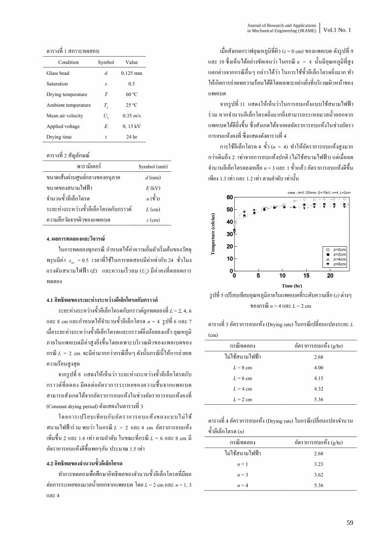
Journal of Research and Applications
in Mechanical Engineering (JRAME) Vol.1 No. 1
59
ตารางท 1 สภาวะทดสอบ Condition Symbol Value
Glass bead d 0.125 mm Saturation s 0.5 Drying temperature T 60 ºC Ambient temperature Ta 25 ºC Mean air velocity Ub 0.35 m/s Applied voltage E 0, 15 kV Drying time t 24 hr
ตารางท 2 สญลกษณ พารามเตอร Symbol (unit)
ขนาดเสนผานศนยกลางของอนภาค d (mm) ขนาดของสนามไฟฟา E (kV) จ านวนขวอเลกโตรด n (ขว) ระยะหางระหวางขวอเลกโตรดกบกราวด L (cm) ความลกวดจากผวของแพคเบด z (cm)
4. ผลการทดลองและวจารณ ในการทดลองทกกรณ ก าหนดใหคาความอมตวเรมตนของวสด
พรนมคา sint = 0.5 เวลาทใชในการทดสอบมคาเทากบ 24 ชวโมง แรงดนสนามไฟฟา (E) และความเรวลม (Ub) มคาคงทตลอดการทดลอง
4.1 อทธพลของระยะหางระหวางอเลกโตรดกบกราวด ระยะหางระหวางขวอเลกโตรดกบกราวดถกทดลองท L = 2, 4, 6
และ 8 cm และก าหนดใหจ านวนขวอเลกโตรด n = 4 รปท 6 และ 7 เมอระยะหางระหวางขวอเลกโตรดและกราวดยงนอยลงแลว อณหภมภายในแพคเบดมคาสงยงขนโดยเฉพาะบรเวณผวของแพคเบดของกรณ L = 2 cm จะมคามากกวากรณอนๆ ดงนนกรณนใหการถายเทความรอนสงสด
จากรปท 8 แสดงใหเหนวา ระยะหางระหวางขวอเลกโตรดกบกราวดทลดลง มผลตออตราการระเหยของความชนจากแพคเบด สามารถสงเกตไดจากอตราการอบแหงในชวงอตราการอบแหงคงท (Constant drying period) ดงแสดงในตารางท 3
โดยการเปรยบเทยบกบอตราการอบแหงของแบบไมใชสนามไฟฟารวม พบวา ในกรณ L = 2 และ 4 cm อตราการอบแหงเพมขน 2 และ 1.6 เทา ตามล าดบ ในขณะทกรณ L = 6 และ 8 cm มอตราการอบแหงดขนพอๆกน ประมาณ 1.5 เทา
4.2 อทธพลของจ านวนขวอเลกโตรด ท าการทดลองเพอศกษาอทธพลของจ านวนขวอเลกโตรดทมผล
ตอการระเหยของมวลน าออกจากแพคเบด โดย L = 2 cm และ n = 1, 3 และ 4
เมอสงเกตกราฟอณหภมทผว (z = 0 cm) ของแพคเบด ดงรปท 9 และ 10 ซงเหนไดอยางชดเจนวา ในกรณ n = 4 นนมอณหภมทสงแตกตางจากกรณอนๆ กลาวไดวา ในการใชขวอเลกโตรดยงมาก ท าใหเกดการถายเทความรอนไดดโดยเฉพาะอยางยงทบรเวณผวหนาของแพคเบด
จากรปท 11 แสดงใหเหนวาในการอบแหงแบบใชสนามไฟฟารวม หากจ านวนอเลกโตรดยงมากยงสามารถระเหยมวลน าออกจากแพคเบดไดดยงขน ซงสงเกตไดจากผลอตราการอบแหงในชวงอตราการอบแหงคงท ซงแสดงดงตารางท 4
การใชอเลกโตรด 4 ขว (n = 4) ท าใหอตราการอบแหงสงมากกวาเดมถง 2 เทาจากการอบแหงปกต (ไมใชสนามไฟฟา) แตเมอลดจ านวนอเลกโตรดลงเหลอ n = 3 และ 1 ขวแลว อตราการอบแหงดขนเพยง 1.3 เทา และ 1.2 เทา ตามล าดบ เทานน
รปท 5 เปรยบเทยบอณหภมภายในแพคเบดทระดบความลก (z) ตางๆ ของกรณ n = 4 และ L = 2 cm
ตารางท 3 อตราการอบแหง (Drying rate) ในกรณเปลยนแปลงระยะ L (cm)
กรณทดลอง อตราการอบแหง (g/hr) ไมใชสนามไฟฟา 2.68
L = 8 cm 4.00 L = 6 cm 4.15 L = 4 cm 4.32 L = 2 cm 5.36
ตารางท 4 อตราการอบแหง (Drying rate) ในกรณเปลยนแปลงจ านวนขวอเลกโตรด (n)
กรณทดลอง อตราการอบแหง (g/hr) ไมใชสนามไฟฟา 2.68
n = 1 3.23 n = 3 3.62 n = 4 5.36
60
50
40
30
20
10
0
Tem
per
ture
(ce
lciu
s)
20151050
Time (hr)
case : d=0.125mm, E=15kV, n=4, L=2cm
z=0cm
z=2cm
z=4cm
z=6cm
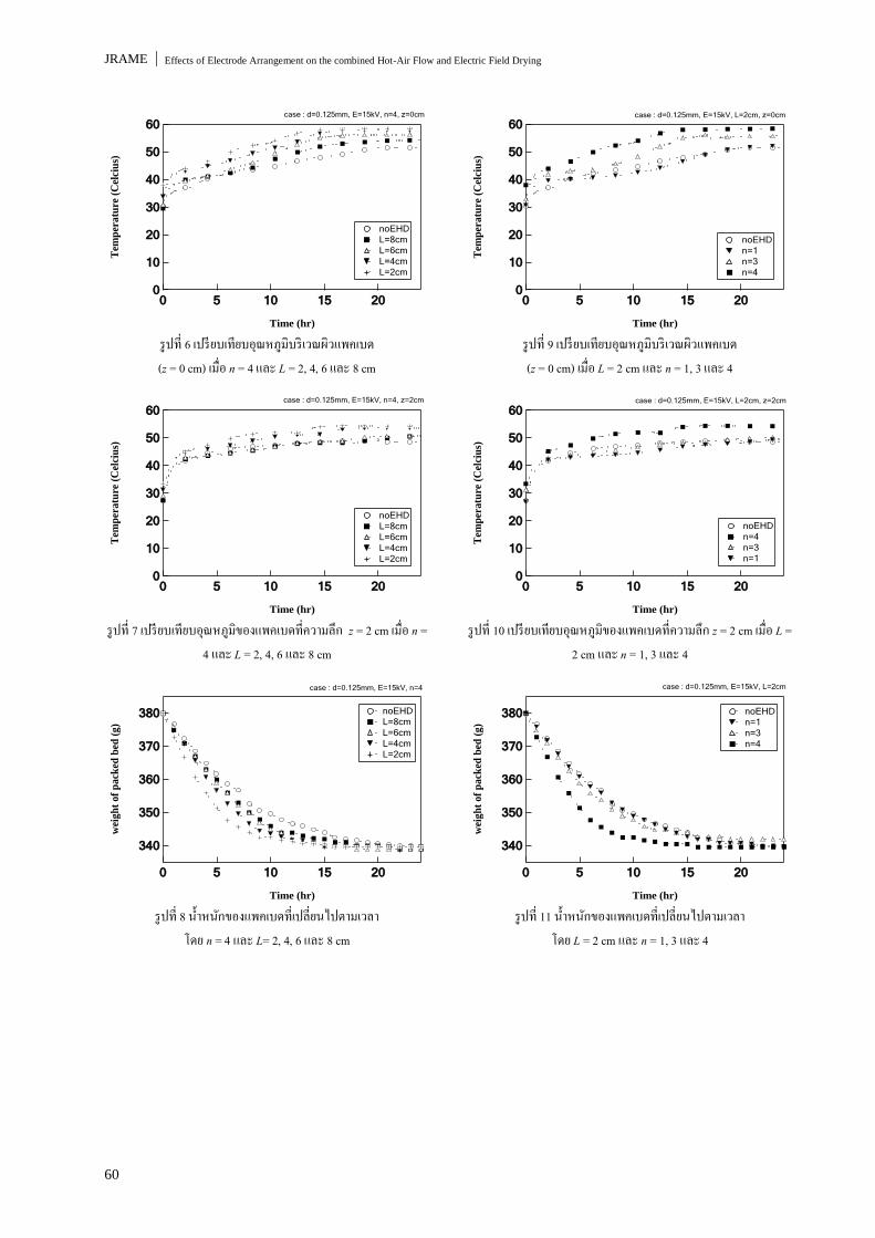
JRAME Effects of Electrode Arrangement on the combined Hot-Air Flow and Electric Field Drying
60
รปท 6 เปรยบเทยบอณหภมบรเวณผวแพคเบด (z = 0 cm) เมอ n = 4 และ L = 2, 4, 6 และ 8 cm
รปท 7 เปรยบเทยบอณหภมของแพคเบดทความลก z = 2 cm เมอ n =
4 และ L = 2, 4, 6 และ 8 cm
รปท 8 น าหนกของแพคเบดทเปลยนไปตามเวลา
โดย n = 4 และ L= 2, 4, 6 และ 8 cm
รปท 9 เปรยบเทยบอณหภมบรเวณผวแพคเบด (z = 0 cm) เมอ L = 2 cm และ n = 1, 3 และ 4
รปท 10 เปรยบเทยบอณหภมของแพคเบดทความลก z = 2 cm เมอ L =
2 cm และ n = 1, 3 และ 4
รปท 11 น าหนกของแพคเบดทเปลยนไปตามเวลา
โดย L = 2 cm และ n = 1, 3 และ 4
60
50
40
30
20
10
0
Tem
per
atu
re (
Cel
ciu
s)
20151050
Time (hr)
case : d=0.125mm, E=15kV, n=4, z=0cm
noEHD
L=8cm
L=6cm
L=4cm
L=2cm
60
50
40
30
20
10
0
Tem
per
atu
re (
Cel
ciu
s)
20151050
Time (hr)
case : d=0.125mm, E=15kV, n=4, z=2cm
noEHD
L=8cm
L=6cm
L=4cm
L=2cm
380
370
360
350
340
wei
gh
t o
f p
ack
ed b
ed (
g)
20151050
Time (hr)
case : d=0.125mm, E=15kV, n=4
noEHD
L=8cm
L=6cm
L=4cm
L=2cm
60
50
40
30
20
10
0
Tem
per
atu
re (
Cel
ciu
s)
20151050
Time (hr)
noEHD
n=1
n=3
n=4
case : d=0.125mm, E=15kV, L=2cm, z=0cm
60
50
40
30
20
10
0
Tem
per
atu
re (
Cel
ciu
s)
20151050
Time (hr)
case : d=0.125mm, E=15kV, L=2cm, z=2cm
noEHD
n=4
n=3
n=1
380
370
360
350
340
wei
gh
t o
f p
ack
ed b
ed (
g)
20151050
Time (hr)
noEHD
n=1
n=3
n=4
case : d=0.125mm, E=15kV, L=2cm
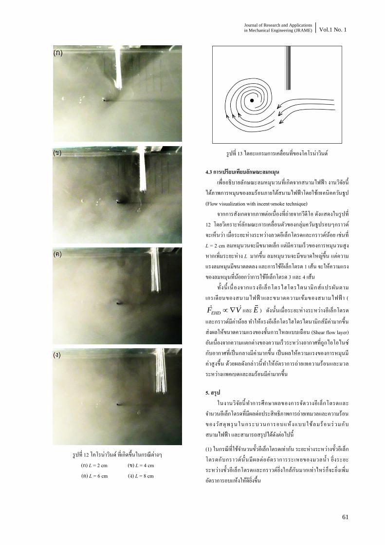
Journal of Research and Applications
in Mechanical Engineering (JRAME) Vol.1 No. 1
61
รปท 12 โคโรนาวนด ทเกดขนในกรณตางๆ
(ก) L = 2 cm (ข) L = 4 cm (ค) L = 6 cm (ง) L = 8 cm
รปท 13 ไดอะแกรมการเคลอนทของโคโรนาวนด
4.3 การเปรยบเทยบลกษณะลมหมน เพออธบายลกษณะลมหมนวนทเกดจากสนามไฟฟา งานวจยน
ไดภาพการหมนของลมรอนภายใตสนามไฟฟาโดยใชเทคนคควนธป (Flow visualization with incent-smoke technique)
จากการสงเกตจากภาพตอเนองทถายจากวดโอ ดงแสดงในรปท 12 โดยวเคราะหลกษณะการเคลอนตวของกลมควนธปรอบๆกราวดจะเหนวา เมอระยะหางระหวางลวดอเลกโตรดและกราวดนอย เชนท L = 2 cm ลมหมนวนจะมขนาดเลก แตมความเรวของการหมนวนสง หากเพมระยะหาง L มากขน ลมหมนวนจะมขนาดใหญขน แตความแรงลมหมนมขนาดลดลง และการใชอเลกโตรด 1 เสน จะใหความแรงของลมหมนทนอยกวาการใชอเลกโตรด 3 และ 4 เสน
ท งน เ นองจากแรงอเลกโตรไฮโดรไดนามกสแปรผนตามเกรเดยนของสนามไฟฟาและขนาดความเขมของสนามไฟฟา (
EHDF V และ E ) ดงนนเมอระยะหางระหวางอเลกโตรดและกราวดมคานอย ท าใหแรงอเลกโตรไฮโดรไดนามกสมคามากขน สงผลใหขนาดความแรงของชนการไหลแบบเฉอน (Shear flow layer) อนเนองจากความแตกตางของความเรวระหวางอากาศทถกไอโอไนซกบอากาศทเปนกลางมคามากขน เปนผลใหความแรงของการหมนมคาสงขน ดวยผลดงกลาวนท าใหอตราการถายเทความรอนและมวลระหวางแพคเบดและลมรอนมคามากขน
5. สรป ในงานวจยนท าการศกษาผลของการจดวางอเลกโตรดและ
จ านวนอเลกโตรดทมผลตอประสทธภาพการถายเทมวลและความรอนของวสดพรนในกระบวนการอบแหงแบบใชลมรอนรวมกบสนามไฟฟา และสามารถสรปไดดงตอไปน
(1) ในกรณทใชจ านวนขวอเลกโตรดเทากน ระยะหางระหวางขวอเลกโตรดกบกราวดน นมผลตออตราการระเหยของมวลน า ยงระยะระหวางขวอเลกโตรดและกราวดยงใกลกนมากเทาไหรกจะยงเพมอตราการอบแหงใหดยงขน
JRAME Effects of Electrode Arrangement on the combined Hot-Air Flow and Electric Field Drying
62
(2) กรณระยะของขวอเลกโตรดและกราวดเทากน จ านวนขวอเลกโตรดทใชมผลตออตราการระเหยของมวลน าเปนอยางมาก ยงจ านวนอเลกโตรดมากยงเพมประสทธภาพการอบแหง เมอเปรยบเทยบกบการอบแหงแบบไมใชสนามไฟฟา การใชอเลกโตรด 4 ขว มอตราการอบแหงดขน 2 เทา ในขณะท การใชอเลกโตรด 3 หรอ 1 ขว มอตราการอบแหงทดขนประมาณ 1.3 เทา
(3) อทธพลของโคโรนาวนดท าใหความชนทผวหนาของแพคเบดสามารถระเหยไปสลมรอนไดเรวขนและท าใหอณหภมภายในแพคเบดมคาสงเรวขน ซงเมอระยะระหวางขวอเลกโตรดกบกราวดทยงเขาใกลกนมาก ท าใหโคโรนาวนดทเกดขนมขนาดเลกแตหมนแรงขน และเมอใชจ านวนขวอเลกโตรดทมากขน กจะท าใหเกดปรากฏการณโคโรนาวนดทซบซอนมากขน ซงเปนผลท าใหเกดการถายเทความรอนจากลมรอนสแพคเบดไดดขน
6. กตตกรรมประกาศ ขอขอบคณคณะวศวกรรมศาสตร มหาวทยาลย ธรรมศาสตร และทนส านกงานคณะกรรมการวจยแหงชาต (วช.) รวมทงโครงการสงเสรมการวจยในอดมศกษาและการพฒนามหาวทยาลยวจยแหงชาตของส านกงานคณะกรรมการอดมศกษาทใหการสนบสนนเงนทนส าหรบการวจย
7. เอกสารอางอง [1] Lai, F.C., Lai, K.W., 2002. EHD enhanced drying with
wire electrode. Drying Technology, Vol. 20, No. 7,
pp. 1393-1405.
[2] Lai, F.C., Sharma, R.K., 2005. EHD Enhanced drying
with multiple needle electrodes. J. Electrostatics, Vol. 63,
pp. 223-237.
[3] Yabe, A., Mori, Y., Hijikata, K., 1996. Active heat
transfer enhancement by utilizing electric fields. Ann
Reviews of Heat Transfer, Vol. 7, pp. 193-244.
[4] Chaktranond, C., Ratanadecho, P., Smathiwat, P.,
Amornvareesaman, P., Pradipasena, T., 2007. Enhancement
of Mass and Heat Transfer in the Unsaturated Double-layer
Packed-bed with Electric fields. In: Proceedings of the 22nd
National Mechanical Engineering Conference. Thammasat
University, Pathumtani, Thailand, No.TSF-044, pp.424-429.
[5] ไชยณรงค จกรธรานนท และ ผดงศกด รตนเดโช. 2552. อทธพลของสนามไฟฟาตอการถายเทมวลและความรอนในวสดพรน. การประชมวชาการเรอง การถายเทพลงงานความรอนและมวลในอปกรณดานความรอน (ครงท 8),โรงแรมโพธวดล รสอรท แอนด สปา จงหวดเชยงราย
[6] Chaktranond, C., Rattanadecho, P., 2009, Heat and Mass
Transfer Enhancement in Unsaturated Porous Packed beds
subjected to Electrohydrodynamics (EHD), In: Proceedings
of the 6th Asia-Pacific Drying Conference (ADC2009),
Bangkok, Thailand.
[7] Chaktranond, C., Rattanadecho, P., 2010. Analysis of
heat and mass transfer enhancement in porous material
subjected to electric fields (effects of particle sizes and
layered arrangement), Experimental Thermal and Fluid
Science 34, pp. 1049-1056.
*ผตดตอ: E-Mail: [email protected], โทรศพท: 044 22 4410, โทรสาร: 044 22 4613
Vol. 1 No.1 TSME | Journal of Research and Applications in Mechanical Engineering
รหสวธเชงพนธกรรมเพอคดเลอกแบบจ าลองการอบแหงขาวเปลอก ส าหรบเครองอบแหงแบบขาวหลนอสระ
Genetic algorithm for the selection of rough rice drying model
for the free-fall paddy dryer
โศรฎา แขงการ1, สพชฌาย มสขเจาส าราญ1 และ ทวช จตรสมบรณ*1
1สาขาวชาวศวกรรมเครองกล ส านกวชาวศวกรรมศาสตร มหาวทยาลยเทคโนโลยสรนาร จ.นครราชสมา 30000 บทคดยอ
งานวจยนท าการคนหาแบบจ าลองทางคณตศาสตรของการอบแหงทเหมาะสมกบการอบแหงขาวเปลอก ดวยเครองอบแหงแบบขาวหลนอสระ โดยท าการอบแหงขาวเปลอกดวยอณหภมอากาศอบแหง 100, 130 และ 150C ใชความเรวของอากาศอบแหง 2 m/s และระยะเวลาพกขาวเปลอก 1 นาทตอรอบการอบแหง จากนนใชรหสวธเชงพนธกรรม (Genetic Algorithm) เพอคนหาคาปจจยของแบบจ าลองทางคณตศาสตรการอบแหงชนบางในรปแบบตางๆ 9 รปแบบ ทสอดคลองกบผลการทดลองอบแหงมากทสด ทงนโดยใช GA Toolbox ของโปรแกรม MATLAB จากการวเคราะหเชงสถตแสดงใหเหนวาแบบจ าลองอบแหงชนบางของ Midilli เหมาะสมทสดในกรณความชนสมพทธอากาศแวดลอมทมคาสง และแบบจ าลองอบแหงชนบางแบบ Two-term exponential เหมาะสมทสดในกรณความชนสมพทธอากาศแวดลอมทมคาต า
ค าหลก: รหสวธเชงพนธกรรม, แบบจ าลองการอบแหงชนบาง, เครองอบแหงแบบขาวหลนอสระ
Abstract
The purpose of this study was to seek the proper thin-layer rough rice model for the free-fall dryer. Experimental data for
drying temperatures 100, 130 and 150C, drying velocity 2 m/s and rest period between drying round of 1 minute were fitted into
the 9 theoretical models by a genetic algorithm (GA). The GA Toolbox in MATLAB was used to generate the correlation
coefficients of the models. The best fitting of the experimental data by these models was specified by comparing the correlation
coefficients, standard errors and mean square deviations. The Midilli model was found to be the most suitable model for drying
condition at high relative humidity of ambient air while the Two-term exponential model was most appropriate for ambient air of
low relative humidity.
Keywords: emissions/ fluidized-bed/ rice husk/ vortex
1. บทน า ขาวเปลอกทไดจากการเกบเกยวมกมความชนในเมลดสง ซง
สงผลตออายการเกบรกษา อตราการเสอมคณภาพ การเขาท าลายของแมลง และเชอรา ดงนนจงตองลดความชนเมลดใหเรวทสด การลดความชนดวยเครองอบแหงเปนทางเลอกหนงทเหมาะสมกบสภาพในปจจบน เนองจากสามารถลดความชนไดอยางรวดเรว ในปรมาณทมาก และในระยะเวลาทก าหนดไดแนนอน โดยไม ขนกบสภาพภมอากาศ แตเนองจากการอบแหงเปนกระบวนการทใชพลงงานสง และความรอนทใชยงมผลตอคณภาพขาวเปลอก จงเกดงานวจยและพฒนาเครองอบแหงขาวเปลอกเพอลดการใชพลงงานและคงรกษาคณภาพขาวเปลอกทด ผลของงานวจยกอให เกดเครองอบแหงขาวเปลอกดวยเทคนคตาง ๆ อยางหลากหลาย เชน เครองอบแหงแบบฟลอดไดซเบด, แบบสเปาเตดเบด, แบบไหลคลกเคลา(LSU), แบบการไหลขวาง และแบบขาวหลนอสระเปนตน
การจ าลองกระบวนการอบแหงเปนสงทส าคญตอการวจยและพฒนาเครองอบแหง โดยสมการท านายความชนภายในวสดเปนหวใจส าคญของระบบสมการอบแหง และเนองจากขาวเปลอกเปนวสดทางชวภาพ ทมความซบซอนในกระบวนการแพรและการระเหยน าภายในเมลด เชนมทงการแพรของน าในสภาพของเหลวและไอ การดดซมดวยระบบคาปลาร และการไหลแบบโมเลกลอสระ (Knudsen flow) ดงนนการสรางสมการท านายความชนภายในขาวเปลอก จงมกใชผลการทดลองอบแหงเปนขอมลในการสรางสมการ โดยเปรยบเทยบผลการทดลองอบแหงเขากบแบบจ าลองอบแหงชนบาง (Thin Layer Drying Model) ซงมหลายรปแบบ ดงแสดงในตารางท 1.
การเปรยบเทยบผลการทดลองกบแบบจ าลองอบแหงชนบาง กคอการหาคาพารามเตอรของแบบจ าลองอบแหงช นบาง ซงท าใหแบบจ าลองสามารถท านายลกษณะการลดลงของความชนขาวเปลอกไดสอดคลองกบผลการทดลองมากทสด เ มอพจารณาจะพบวา

JRAME Genetic algorithm for the selection of rough rice drying model for the free-fall paddy dryer
64
กระบวนการดงก ล าว ค อ ปญหาการหาค า ท เหมาะสม ท สด (Optimization Problem) นนเอง ซงในปจจบนเทคนคการคนหาค าตอบดวยรหสวธเชงพนธกรรม (genetic algorithm) ก าลงไดรบการประยกตใชอยางมากมายในหลากหลายงาน เนองจากเปนทยอมรบวาสามารถหลกเลยงค าตอบแบบวงแคบเฉพาะถน (local optimum) และสามารถคนหาค าตอบทใกลเคยงกบค าตอบทเหมาะสมทสดแบบวงกวาง (near global optimum) ได
เพอการวจยและพฒนาเครองอบแหงแบบขาวหลนอสระในขนสงตอไป งานวจยนจงท าการทดลองอบแหงขาวเปลอกดวยเครองอบแหงแบบขาวหลนอสระซงเปนการอบแหงแบบมการพกในระหวางกระบวนการ จากนนน าผลการทดลองทไดมาเปรยบเทยบกบแบบจ าลองอบแหงชนบาง โดยประยกตใชรหสวธพนธกรรมในการคนหาคาพารามเตอรทเหมาะสมทสดของแตละแบบจ าลอง แลวใชการวเคราะหเชงสถตเพอเลอกแบบจ าลองอบแหงชนผวบางทเหมาะสม ซงแบบจ าลองทไดซอนทบกบผลการทดลองแบบมการพกไดด แสดงถงความเหมาะสมของแบบจ าลองในการท านายผลการอบแหงดวยเครองอบแหงแบบขาวหลนอสระ
2. หลกการท างานเครองอบแหงแบบหลนอสระ เครองอบแหงแบบหลนอสระน ไดถกคดคนขน โดยคาดหวงวา
จะสามารถอบแหงไดอยางรวดเรว ประหยดพลงงาน และไมเกดผลเสยหายตอเมลดขาว ซงจะท าใหไดขาวเตมเมลด (ขาวตน) เปนปรมาณสง อกทงไดคณภาพดทงในดานของกลนและสของขาวสาร ซงเครองอบนไดรบการจดสทธบตรแลว [3]
รปท 1 แสดงใหเหนถงหลกการท างานของเครองอบแหงนคอ พดลมเปาอากาศผานอปกรณสรางความรอน เพอสรางลมรอนเขาสดานลางของทออบแหงทตงอยในแนวดง สวนขาวเปลอกชนตกลงมาโดยอสระจากดานบนของทออบแหงสวนทางกบการไหลขนของลมรอน ท าใหเกดการแลกเปลยนความรอนและความชนกบอากาศรอนอยางรวดเรว ท าใหขาวเปลอกแหงลงอยางรวดเรว แตขาวเปลอกจะอยในทออบแหงเปนระยะเวลาสนๆ เพยงประมาณ 1 วนาทในแตละรอบ (กรณเครองอบแหงขนาดหองทดลอง ททออบแหงยาวประมาณ 2 เมตร แตถาทออบแหงยาวกวานกจะมเวลามากกวาน) จากน นขาวเปลอกจะออกจากทออบแหงเขาสถงพกทางดานลาง
เครองอบแหงนแตกตางจากเครองอบแหง แบบ LSU ทถงแมจะมการไหลของเมลดพชในแนวดงสวนทางกบอากาศแตจะมตวควบคมการไหลใหเมลดพชตกลงดานลางอยางชาๆ โดยอากาศจะคอยๆ ซมผานขนไปดานบน แตเครองอบแหงแบบใหมนเมลดพชตกลงสวนทางกบอากาศในแนวดงดวยความเรวสงและมความพรนเมลดขาวสง ท าใหพนทสมผสในการถายเทความรอนและความชนเพมมากขน ทส าคญคอความเรวสมพทธระหวางอากาศกบเมลดพชในเครองอบแหงนจะมคาสง โดยความเรวของอากาศไมจ าเปนตองมคาสงมากนก (ต ากวาความเรวลอยตว) ซงท าใหมอตราการถายเทมวลความชนทสงเปนสดสวนกน
เพอใหไดขาวเปลอกทมความชนอยในระดบทเหมาะสมตอการจดเกบจงตองล าเลยงขาวเปลอกเขาสทออบแหงหลายรอบ ดงนนจงเกดชวงเวลาทขาวเปลอกรอทจะเขาสทออบแหงอกครง เรยกชวงเวลานวา ‘การพก’ (resting period) นนคอระยะเวลาตงแตขาวเปลอกออกจากทออบ เขาสถงพกดานลาง และถกล าเลยงขนจนกระทงเขาสทออบแหงอกครง ชวงระยะเวลาดงกลาวจะมากหรอนอยขนกบปรมาณขาวเปลอกในถงพกดานลาง ผลการวจยทผานมาแสดงใหเหนวาเครองอบแหงแบบขาวหลนอสระมอตราการอบแหงทคอนขางสง อยในชวง 0.0514-0.0971 (%w.b./sec.) [5] และใชพลงงานปฐมภมจ าเพาะทต า อยในชวง 3.00-3.55 MJ/kg water evap. [6] โดยสามารถคงรกษาปรมาณขาวตนไดสงถงประมาณ 55% [7]
เครองอบแหงทใชในการวจยนเปนเครองระดบหองทดลองขนาดเลก โดยมทออบแหงขนาดวงใน 8 เซนตเมตร ความยาวทอรวม 210 เซนตเมตร ขดลวดความรอนขนาด 6 กโลวตต มอเตอรพดลมขนาด 1.75 กโลวตต ซงสามารถปรบแตงความรอนและจ านวนรอบพดลมไดอยางตอเนอง
รปท 1 โครงรางเครองอบแหงแบบขาวหลนอสระ 3.แบบจ าลองอบแหงชนผวบาง
แบบจ าลองทางคณตศาสตรสวนมากทใชในการศกษาเกยวกบการอบแหงชนบาง แสดงในตารางท 1 โดยแตละสมการถกสรางขน
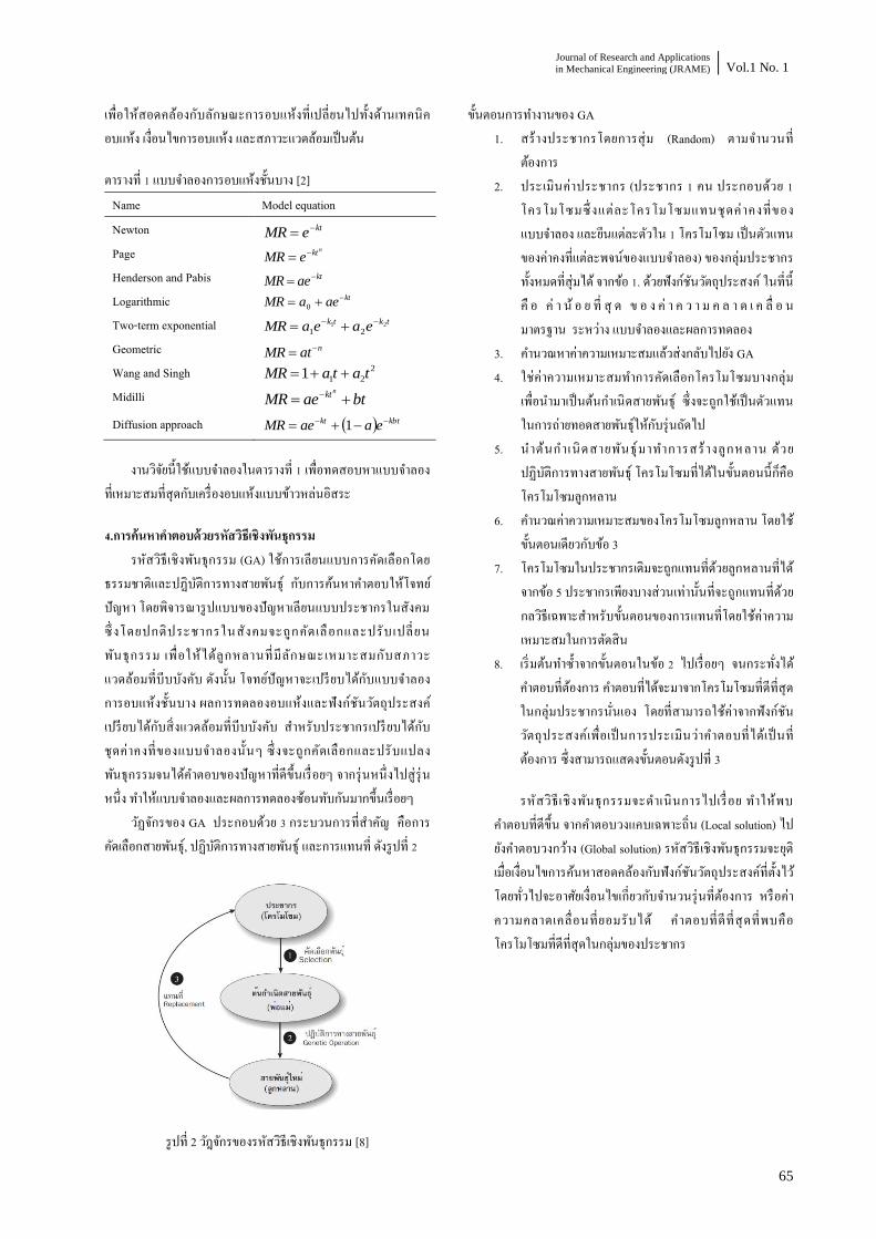
Journal of Research and Applications
in Mechanical Engineering (JRAME) Vol.1 No. 1
65
เพอใหสอดคลองกบลกษณะการอบแหงทเปลยนไปทงดานเทคนคอบแหง เงอนไขการอบแหง และสภาวะแวดลอมเปนตน
ตารางท 1 แบบจ าลองการอบแหงชนบาง [2] Name Model equation Newton kteMR Page nkteMR Henderson and Pabis ktaeMR Logarithmic ktaeaMR 0
Two-term exponential tktk
eaeaMR 21
21
Geometric natMR Wang and Singh 2
211 tataMR Midilli btaeMR
nkt Diffusion approach kbtkt eaaeMR 1
งานวจยนใชแบบจ าลองในตารางท 1 เพอทดสอบหาแบบจ าลองทเหมาะสมทสดกบเครองอบแหงแบบขาวหลนอสระ
4.การคนหาค าตอบดวยรหสวธเชงพนธกรรม รหสวธเชงพนธกรรม (GA) ใชการเลยนแบบการคดเลอกโดย
ธรรมชาตและปฏบตการทางสายพนธ กบการคนหาค าตอบใหโจทยปญหา โดยพจารณารปแบบของปญหาเลยนแบบประชากรในสงคม ซงโดยปกตประชากรในสงคมจะถกคดเลอกและปรบเปลยนพนธกรรม เพอใหไดลกหลานทมลกษณะเหมาะสมกบสภาวะแวดลอมทบบบงคบ ดงนน โจทยปญหาจะเปรยบไดกบแบบจ าลองการอบแหงชนบาง ผลการทดลองอบแหงและฟงกชนวตถประสงคเปรยบไดกบสงแวดลอมทบบบงคบ ส าหรบประชากรเปรยบไดกบชดคาคงทของแบบจ าลองน นๆ ซงจะถกคดเลอกและปรบแปลงพนธกรรมจนไดค าตอบของปญหาทดขนเรอยๆ จากรนหนงไปสรนหนง ท าใหแบบจ าลองและผลการทดลองซอนทบกนมากขนเรอยๆ
วฏจกรของ GA ประกอบดวย 3 กระบวนการทส าคญ คอการคดเลอกสายพนธ, ปฏบตการทางสายพนธ และการแทนท ดงรปท 2
รปท 2 วฎจกรของรหสวธเชงพนธกรรม [8]
ขนตอนการท างานของ GA 1. สรางประชากรโดยการสม (Random) ตามจ านวนท
ตองการ 2. ประเมนคาประชากร (ประชากร 1 คน ประกอบดวย 1
โครโมโซมซงแตละโครโมโซมแทนชดคาคงทของแบบจ าลอง และยนแตละตวใน 1 โครโมโซม เปนตวแทนของคาคงทแตละพจนของแบบจ าลอง) ของกลมประชากรทงหมดทสมได จากขอ 1. ดวยฟงกชนวตถประสงค ในทน ค อ ค า น อ ย ท ส ด ข อ ง ค า ค ว า ม ค ล า ด เ ค ล อ นมาตรฐาน ระหวาง แบบจ าลองและผลการทดลอง
3. ค านวณหาคาความเหมาะสมแลวสงกลบไปยง GA 4. ใชคาความเหมาะสมท าการคดเลอกโครโมโซมบางกลม
เพอน ามาเปนตนก าเนดสายพนธ ซงจะถกใชเปนตวแทนในการถายทอดสายพนธใหกบรนถดไป
5. น าตนก าเ นดสายพนธมาท าการสรางลกหลาน ดวยปฏบตการทางสายพนธ โครโมโซมทไดในขนตอนนกคอโครโมโซมลกหลาน
6. ค านวณคาความเหมาะสมของโครโมโซมลกหลาน โดยใชขนตอนเดยวกบขอ 3
7. โครโมโซมในประชากรเดมจะถกแทนทดวยลกหลานทไดจากขอ 5 ประชากรเพยงบางสวนเทานนทจะถกแทนทดวยกลวธเฉพาะส าหรบขนตอนของการแทนทโดยใชคาความเหมาะสมในการตดสน
8. เรมตนท าซ าจากขนตอนในขอ 2 ไปเรอยๆ จนกระทงได ค าตอบทตองการ ค าตอบทไดจะมาจากโครโมโซมทดทสดในกลมประชากรนนเอง โดยทสามารถใชคาจากฟงกชนวตถประสงคเพอเปนการประเมนวาค าตอบทไดเปนทตองการ ซงสามารถแสดงขนตอนดงรปท 3
รหสวธเชงพนธกรรมจะด าเนนการไปเรอย ท าใหพบค าตอบทดขน จากค าตอบวงแคบเฉพาะถน (Local solution) ไปยงค าตอบวงกวาง (Global solution) รหสวธเชงพนธกรรมจะยตเมอเงอนไขการคนหาสอดคลองกบฟงกชนวตถประสงคทตงไว โดยทวไปจะอาศยเงอนไขเกยวกบจ านวนรนทตองการ หรอคาความคลาดเคลอนทยอมรบได ค าตอบทดทสดทพบคอโครโมโซมทดทสดในกลมของประชากร
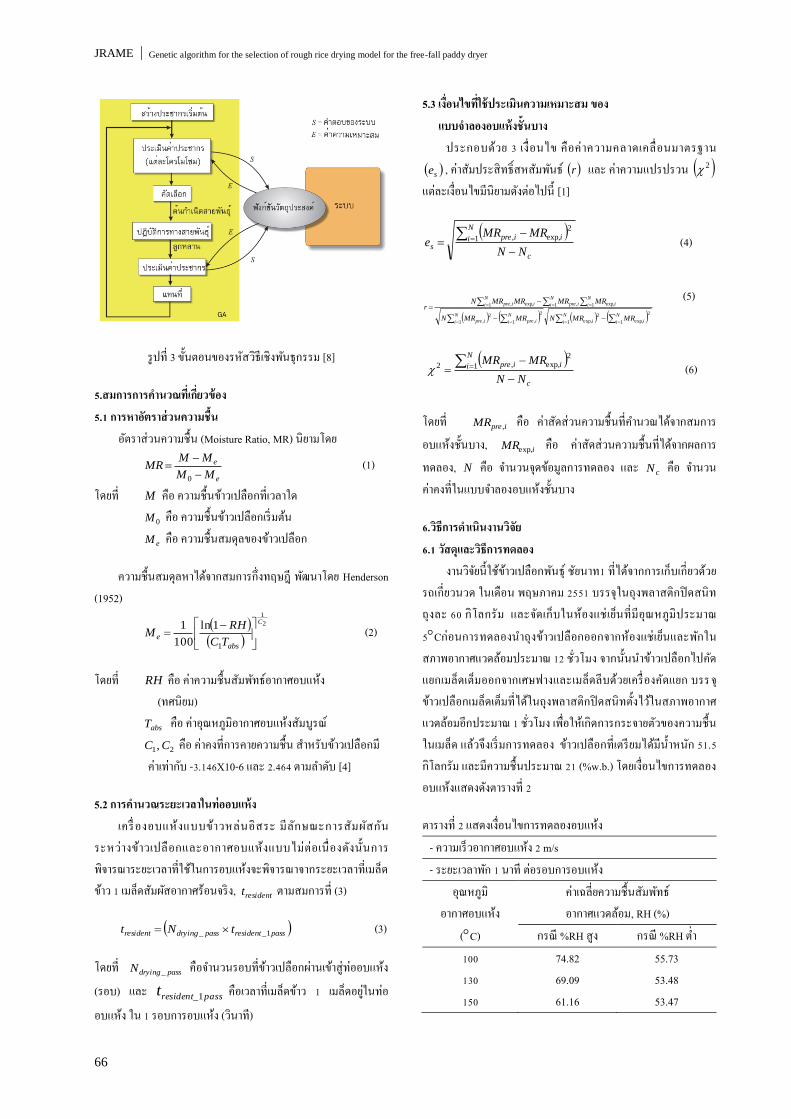
JRAME Genetic algorithm for the selection of rough rice drying model for the free-fall paddy dryer
66
รปท 3 ขนตอนของรหสวธเชงพนธกรรม [8]
5.สมการการค านวณทเกยวของ 5.1 การหาอตราสวนความชน
อตราสวนความชน (Moisture Ratio, MR) นยามโดย
e
e
MM
MMMR
0
(1)
โดยท M คอ ความชนขาวเปลอกทเวลาใด 0M คอ ความชนขาวเปลอกเรมตน eM คอ ความชนสมดลของขาวเปลอก
ความชนสมดลหาไดจากสมการกงทฤษฎ พฒนาโดย Henderson (1952)
2
1
1
1ln
100
1 C
abs
eTC
RHM
(2)
โดยท RH คอ คาความชนสมพทธอากาศอบแหง (ทศนยม) absT คอ คาอณหภมอากาศอบแหงสมบรณ
21, CC คอ คาคงทการคายความชน ส าหรบขาวเปลอกม คาเทากบ -3.146X10⁻⁶ และ 2.464 ตามล าดบ [4]
5.2 การค านวณระยะเวลาในทออบแหง เครองอบแหงแบบขาวหลนอสระ มลกษณะการสมผสกน
ระหวางขาวเปลอกและอากาศอบแหงแบบไมตอเนองดงน นการพจารณาระยะเวลาทใชในการอบแหงจะพจารณาจากระยะเวลาทเมลดขาว 1 เมลดสมผสอากาศรอนจรง, residentt ตามสมการท (3)
passresidentpassdryingresident tNt 1__ (3)
โดยท passdryingN _ คอจ านวนรอบทขาวเปลอกผานเขาสทออบแหง
(รอบ) และ passresidentt 1_ คอเวลาทเมลดขาว 1 เมลดอยในทอ
อบแหง ใน 1 รอบการอบแหง (วนาท)
5.3 เงอนไขทใชประเมนความเหมาะสม ของ แบบจ าลองอบแหงชนบาง
ประกอบดวย 3 เงอนไข คอคาความคลาดเคลอนมาตรฐาน se , คาสมประสทธสหสมพนธ r และ คาความแปรปรวน 2 แตละเงอนไขมนยามดงตอไปน [1]
c
N
i iipre
sNN
MRMRe
1
2exp,, (4)
N
i
N
i ii
N
i
N
i ipreipre
N
i
N
i
N
i iipreiipre
MRMRNMRMRN
MRMRMRMRNr
1
2
1 exp,2
exp,1
2
1 ,2
,
1 1 1 exp,,exp,, (5)
c
N
i iipre
NN
MRMR
1
2exp,,2 (6)
โดยท ipreMR , คอ คาสดสวนความชนทค านวณไดจากสมการอบแหงชนบาง, iMRexp, คอ คาสดสวนความชนทไดจากผลการทดลอง, N คอ จ านวนจดขอมลการทดลอง และ cN คอ จ านวนคาคงทในแบบจ าลองอบแหงชนบาง
6.วธการด าเนนงานวจย 6.1 วสดและวธการทดลอง
งานวจยนใชขาวเปลอกพนธ ชยนาท1 ทไดจากการเกบเกยวดวยรถเกยวนวด ในเดอน พฤษภาคม 2551 บรรจในถงพลาสตกปดสนท ถงละ 60 กโลกรม และจดเกบในหองแชเยนทมอณหภมประมาณ 5Cกอนการทดลองน าถงขาวเปลอกออกจากหองแชเยนและพกในสภาพอากาศแวดลอมประมาณ 12 ชวโมง จากนนน าขาวเปลอกไปคดแยกเมลดเตมออกจากเศษฟางและเมลดลบดวยเครองคดแยก บรร จขาวเปลอกเมลดเตมทไดในถงพลาสตกปดสนทตงไวในสภาพอากาศแวดลอมอกประมาณ 1 ชวโมง เพอใหเกดการกระจายตวของความชนในเมลด แลวจงเรมการทดลอง ขาวเปลอกทเตรยมไดมน าหนก 51.5 กโลกรม และมความชนประมาณ 21 (%w.b.) โดยเงอนไขการทดลองอบแหงแสดงดงตารางท 2
ตารางท 2 แสดงเงอนไขการทดลองอบแหง - ความเรวอากาศอบแหง 2 m/s - ระยะเวลาพก 1 นาท ตอรอบการอบแหง
อณหภม อากาศอบแหง
(C)
คาเฉลยความชนสมพทธ อากาศแวดลอม, RH (%)
กรณ %RH สง กรณ %RH ต า 100 74.82 55.73 130 69.09 53.48 150 61.16 53.47

Journal of Research and Applications
in Mechanical Engineering (JRAME) Vol.1 No. 1
67
เรมการทดลอง ดวยการเปดพดลม กะพอล าเลยงและเครองท าความรอน ตงความเรวและอณหภมอากาศอบแหงตามเงอนไขขางตน เกบตวอยางเรมตน 15 กรม ในถงพลาสตกปดสนท น าขาวเปลอกทเตรยมไวเทใสถงพกดานบน ขาวเปลอกจะไหลผานทออบแหง เขาสถงพกดานลาง และเขาสกะพอล าเลยง เพอล าเลยงกลบไปถงพกดานบน เกดการอบแหงซ าเปนวงรอบตามวธการขางตนจนกระทง ขาวเปลอกไดความชนประมาณ 13% (w.b.) ในขณะอบแหงเกบตวอยางขาวเปลอกตวอยางละ 15 กรมในถงพลาสตกปดสนท โดยเกบทกๆ 5 นาท ในชวโมงแรกและทกๆ 10 นาทในชวโมงตอมา เพอน าไปหาคาความชน หลงจากเสรจสนกระบวนการอบแหงน าตวอยางทเกบไดพกในอณหภมบรรยากาศประมาณ 6 ชวโมง เพอใหอณหภมขาวเปลอกลดลง คลายความเครยดทผวและเกดการกระจายความชนอยางสม าเสมอตลอดเมลดขาว จากนนน าไปหาคาความชนโดยวธการอบดวยตอบ (Oven Method) โดยน าขาวเปลอกตวอยางทงเมลด น าไปอบในตอบทอณหภม 103C เปนเวลา 72 ชวโมง
6.2 ฟงคชนคาความเหมาะสมและเงอนไขรหสวธพนธกรรม ผวจยเลอกใช Genetic Algorithm Tool ของโปรแกรม
MATLAB ซงอยในรปแบบ Graphic User Interface, GUI การใชงานเรมตนจากการสรางฟงคชนคาความเหมาะสม (ฟงคชนวตถประสงค) ในรปของ m-file โดยงานวจยนใชคาความคลาดเคลอนมาตรฐาน se เปนคาความเหมาะสมทตองการใหมคานอยทสด ซง se ไดจากความคลาดเคลอนระหวางคาสดสวนความชนทไดจากการทดลองกบทไดจากแบบจ าลองอบแหงชนบาง ตามสมการท 4
อนดบตอมาท าการก าหนดกลยทธ วว ฒนาการ (Evolution Strategies) ซงผวจยไดเลอกใชตามทแสดงในตารางท 3 จากนนท าการ run โปรแกรมผาน Genetic Algorithm Tool ทายทสดไดค าตอบเปนคาของตวแปรในแบบจ าลองอบแหงช นบางทพจารณา ซงมคาความคลาดเคลอนมาตรฐานต าทสด
ตารางท 3 แสดงกลยทธววฒนาการทเลอกใช Population size - 3000 Fitness scaling - Rank Selection - Stochastic uniform Reproduction - Elite count: 2
- Crossover fraction: 0.8 Mutation - Gaussian function Crossover - Heuristic Migration - Forward Hybrid function - fminsearch Stopping criteria - 300,000 Generation
7.ผลการค านวณและการวจารณผล คาตวแปรของแบบจ าลองอบแหงชนบางทง 9 สมการ ทคนหา
ดวย GA และผลการวเคราะหเชงสถต ในกรณความชนสมพทธอากาศแวดลอมสงแสดงในตารางท 4-7 และในกรณความชนสมพทธอากาศแวดลอมต าแสดงในตารางท 8-10
แบบจ าลองอบแหงทดจะตองมคาสมประสทธสหสมพนธ r เขาใกล 1 และมคาความคลาดเคลอนมาตรฐาน se และคาเฉลยเบยงเบนมาตรฐาน 2 ทต า
จากตารางท 4-6 แสดงใหเหนวาแบบจ าลองทเหมาะสมทสดในการอธบายการอบแหงขาวเปลอกดวยเครองอบแหงแบบขาวหลนอสระ เมอความชนสมพทธอากาศแวดลอมสงคอ แบบจ าลองของ Midilli โดยในการทดลองทง 3 กรณ มคา r ต าทสดเทากบ 0.999480 และมคา es สงสดเทากบ 0.005975 และคา 2 สงทสดเทากบ 0.00004 ถงแมวาในกรณท 150C คา es ทไดจากแบบจ าลองของ Midilli จะมคา0.005975 ซงมากกวาแบบจ าลองแบบ Two-term exponential (es = 0.005842) และเสนกราฟของแบบจ าลองทงสองเกาะกบผลการทดลองไดด ดงแสดงในรปท 4 ดงนนจงถอวาทอณหภม 150C สามารถใชแบบจ าลองทงสองได และเลอกใชแบบจ าลองของ Midilli เพอใหเปนแนวทางเดยวกนกบการอบแหงทอณหภมอบแหง 100C และ 130C และสามารถหาความสมพนธของคาคงทของสมการกบอณหภมอบแหง ส าหรบกรณความชนสมพทธอากาศแวดลอมสงได
จากตารางท 7-9 แสดงใหเหนวาแบบจ าลองทเหมาะสมทสดในการอธบายการอบแหงขาวเปลอกดวยเครองอบแหงแบบขาวหลนอสระ เมอความชนสมพทธอากาศแวดลอมต าคอ แบบจ าลองแบบ Two-term exponential ซงมคา r ต าสดเทากบ 0.999417 และมคา es สงสดเทากบ 0.006614 และคา 2 สงสดเทากบ 0.000049
เหตผลทางกายภาพทแบบจ าลองของ Midilli มความเหมาะสมกบการอบแหงทความชนสมพทธอากาศแวดลอมสง อาจเนองมาจากคาความดนไอของอากาศทปกคลมกองขาวเปลอกในชวงระยะพกมคาสง สงผลใหความแตกตางระหวางความดนไอภายในกบภายนอกต ากวากรณความชนสมพทธอากาศแวดลอม ต า จงท าใหการกระจายความชนภายในเมลดและการ ระเหยสบรรยากาศเปนไปไดชากวา ลกษณะการลดลงของความชนจงคอนขางราบเรยบ สอดคลองกบรปแบบของแบบจ าลองของ Midilli ทมพจนการลดลงแบบเชงเสนดงแสดงในรปท 4 ในทางกลบกนกรณการอบแหงทความชนสมพทธอากาศแวดลอมต า การ ลดลงของความชนจงรวดเรวและมลกษณะโคงงอมากกวา ดงนนแบบจ าลองแบบ Two-term exponential จงใหความสอดคลองกบผลการทดลองทดกวาดงแสดงในรปท 5
ดงนน กรณความชนสมพทธอากาศแวดลอมสง เลอกแบบจ าลองของ Midilli
btaeMRnkt (7)

JRAME Genetic algorithm for the selection of rough rice drying model for the free-fall paddy dryer
68
โดยทสมประสทธ a, k, n และ b เปนฟงกชนของอณหภมอากาศอบแหง (T) ดงน a = -0.00001133T2 + 0.00292897T + 0.80653797
(8) k = 0.00000039T2 - 0.00007671T + 0.00463167
(9) n = -0.00007536T2 + 0.01611246T + 0.36044789
(10) b = -0.00000036T2 + 0.00008397T - 0.00436890
(11)
กรณความชนสมพทธอากาศแวดลอมต า เลอก แบบจ าลองแบบ Two-term exponential
tktkeaeaMR 21
21
(12)
โดยท สมประสทธ a1, k1, a2และ k2 เปนฟงกชนของอณหภมอากาศอบแหง (T) ดงน
a1 = 0.00018725T2 - 0.03041804T + 2.26215079 (13)
k1 = -0.00000332T2 + 0.00080216T - 0.04427326 (14)
a2 = -0.00017492T2 + 0.02724108T - 1.07857873 (15)
k2 = -0.00000737T2 + 0.00166233T - 0.08351565 (16)
ความถกตองของแบบจ าลองอบแหงและสมการความสมพนธทสรางขน ดวยการเปรยบเทยบกบคาสดสวนความชนทท านายไดกบผลการทดลอง แสดงในรปท 6 และ 7 จากรปพบวาคาทท านายคอนขางซอนทบกบเสนตรง ซงแสดงถงความเหมาะสมของแบบจ าลองอบแหงทงสอง ในการท านายการอบแหงขาวเปลอกเมอใชเครองอบแหงแบบขาวหลนอสระ
8. สรป งานวจยนประยกตใชรหสวธเชงพนธกรรมในการก าหนดคา
ปจจยของแบบจ าลองอบแหงชนบาง 9 แบบ เพอใชกบเครองอบแหงขาวเปลอกแบบขาวหลนอสระ ผลงานวจยแสดงใหเหนวา แบบจ าลองอบแหงชนบางของ Midilli เหมาะสมทสดในกรณความชนสมพทธอากาศแวดลอมทมคาสง และแบบจ าลองอบแหงชนบางแบบ Two-term exponential เหมาะสมทสดในกรณความชนสมพทธอากาศแวดลอมทมคาต า ซง แบบจ าลองทงสองใหคาสมประสทธสหสมพนธทใกลเคยง 1 มาก อกทงคาความคลาดเคลอนมาตรฐาน และคาเฉลย
เบยงเบนมาตรฐานยงต าอกดวย งานวจยนยงไดน าเสนอสมการความสมพนธระหวางปจจยของแบบจ าลองกบอณหภมอากาศอบแหงในรปของสมการโพลโนเมยลเพอใหไดผลการท านายทดทสดอกดวย
9. กตตกรรมประกาศ
งานวจยนไดรบการสนนสนนทนวจยบางสวนจาก ส านกงานคณะกรรมการวจยแหงชาต (วช. ) และสถาบนวจยและพฒนา มหาวทยาลยเทคโนโลยสรนาร
10. เอกสารอางอง [1] Chapra, S.C., Canel, R.P., 1989. Numerical method for engineer. McGraw-Hill Book Company, New York. [2] Vivian, N.P., 2007. Focus on Food Engineering Research and Developments. Nova Science Publishers, New York. [3] กรมทรพยสนทางปญญา, สทธบตรการประดษฐชอ ‚เครองอบแหงแบบการไหลสวนทางในแนวดง‛. เลขทสทธบตร 22985, ออกเมอ ๒๗ ธนวาคม ๒๕๕๐ [4] สมชาต โสภณรณฤทธ. 2540. การอบแหงเมลดพชและอาหารบางประเภท. กรงเทพฯ, สถาบนเทคโนโลยพระจอมเกลาธนบร [5] สพชฌาย มสขเจาส าราญ และ ทวช จตรสมบรณ. 2552. ผลของระยะพก ความเรว และอณหภมตออตราอบแหงในเครองอบแหงแบบขาวเปลอกหลนอสระ, การประชมวชาการสมาคมวศวกรรมเกษตรแหงประเทศไทย ครงท10, มหาวทยาลยเทคโนโลยสรนาร [6] สพชฌาย มสขเจาส าราญ และ ทวช จตรสมบรณ. 2552. ผลของระยะพก อณหภม และความเรวอากาศตอการสนเปลองพลงงานในการอบแหงดวยเครองอบแหงแบบหลนอสระ, การประชมวชาการเครอขายพลงงานแหงประเทศไทย ครงท 5, มหาวทยาลยนเรศวร [7] สพชฌาย มสขเจาส าราญ และ ทวช จตรสมบรณ. 2552. เครองอบแหงแบบหลนอสระ : เงอนไขการอบแหงทใหคณภาพขาวสารทด, การประชมวชาการเครอขายวศวกรรมเครองกลแหงประเทศไทยครงท 23, มหาวทยาลยเชยงใหม [8] อาทตย ศรแกว. 2552. ปญญาเชงค านวณ, สาขาวศวกรรมไฟฟา ส านกวชาวศวกรรมศาสตร มหาวทยาลยเทคโนโลยสรนาร
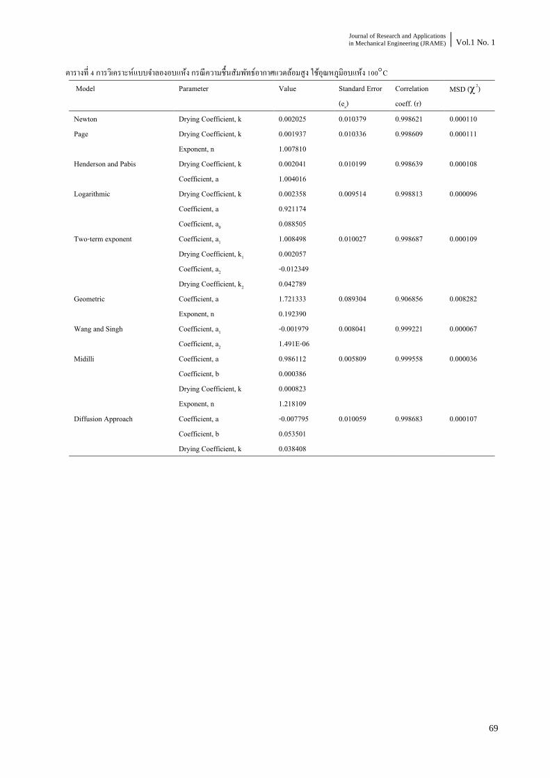
Journal of Research and Applications
in Mechanical Engineering (JRAME) Vol.1 No. 1
69
ตารางท 4 การวเคราะหแบบจ าลองอบแหง กรณความชนสมพทธอากาศแวดลอมสง ใชอณหภมอบแหง 100C Model Parameter Value Standard Error
(es) Correlation coeff. (r)
MSD (2)
Newton Drying Coefficient, k 0.002025 0.010379 0.998621 0.000110 Page Drying Coefficient, k 0.001937 0.010336 0.998609 0.000111
Exponent, n 1.007810 Henderson and Pabis Drying Coefficient, k 0.002041 0.010199 0.998639 0.000108
Coefficient, a 1.004016 Logarithmic Drying Coefficient, k 0.002358 0.009514 0.998813 0.000096
Coefficient, a 0.921174 Coefficient, a0 0.088505
Two-term exponent Coefficient, a1 1.008498 0.010027 0.998687 0.000109 Drying Coefficient, k1 0.002057 Coefficient, a2 -0.012349 Drying Coefficient, k2 0.042789
Geometric Coefficient, a 1.721333 0.089304 0.906856 0.008282 Exponent, n 0.192390
Wang and Singh Coefficient, a1 -0.001979 0.008041 0.999221 0.000067 Coefficient, a2 1.491E-06
Midilli Coefficient, a 0.986112 0.005809 0.999558 0.000036 Coefficient, b 0.000386 Drying Coefficient, k 0.000823 Exponent, n 1.218109
Diffusion Approach Coefficient, a -0.007795 0.010059 0.998683 0.000107 Coefficient, b 0.053501 Drying Coefficient, k 0.038408

JRAME Genetic algorithm for the selection of rough rice drying model for the free-fall paddy dryer
70
ตารางท 5 การวเคราะหแบบจ าลองอบแหง กรณความชนสมพทธอากาศแวดลอมสง ใชอณหภมอบแหง 130C Model Parameter Value Standard Error
(es) Correlation coeff. (r)
MSD (2)
Newton Drying Coefficient, k 0.002025 0.010379 0.998621 0.000110 Page Drying Coefficient, k 0.001852 0.008386 0.999065 0.000074
Exponent, n 1.047085 Henderson and Pabis Drying Coefficient, k 0.002454 0.007948 0.999135 0.000066
Coefficient, a 1.012401 Logarithmic Drying Coefficient, k 0.002574 0.007879 0.999150 0.000067
Coefficient, a 0.982580 Coefficient, a0 0.031457
Two-term exponent Coefficient, a1 1.019035 0.007246 0.999283 0.000058 Drying Coefficient, k1 0.002486 Coefficient, a2 -0.020826 Drying Coefficient, k2 0.062342
Geometric Coefficient, a 1.683932 0.086039 0.915322 0.007755 Exponent, n 0.190412
Wang and Singh Coefficient, a1 -0.002271 0.008351 0.999250 0.000073 Coefficient, a2 1.845E-06
Midilli Coefficient, a 0.995787 0.005266 0.999620 0.000031 Coefficient, b 0.000392 Drying Coefficient, k 0.001186 Exponent, n 1.181532
Diffusion Approach Coefficient, a -0.019029 0.007254 0.999282 0.000056 Coefficient, b 0.042598 Drying Coefficient, k 0.058348
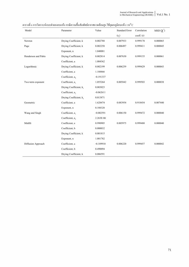
Journal of Research and Applications
in Mechanical Engineering (JRAME) Vol.1 No. 1
71
ตารางท 6 การวเคราะหแบบจ าลองอบแหง กรณความชนสมพทธอากาศแวดลอมสง ใชอณหภมอบแหง 150C Model Parameter Value Standard Error
(es) Correlation coeff. (r)
MSD (2)
Newton Drying Coefficient, k 0.002788 0.007933 0.999178 0.000065 Page Drying Coefficient, k 0.002258 0.006497 0.999411 0.000045
Exponent, n 1.040081 Henderson and Pabis Drying Coefficient, k 0.002814 0.007630 0.999155 0.000061
Coefficient, a 1.004362 Logarithmic Drying Coefficient, k 0.002199 0.006259 0.999429 0.000043
Coefficient, a 1.188866 Coefficient, a0 -0.191337
Two-term exponent Coefficient, a1 1.055264 0.005842 0.999503 0.000038 Drying Coefficient, k1 0.003023 Coefficient, a2 -0.062611 Drying Coefficient, k2 0.013871
Geometric Coefficient, a 1.628474 0.083954 0.918454 0.007440 Exponent, n 0.188328
Wang and Singh Coefficient, a1 -0.002591 0.006150 0.999472 0.000040 Coefficient, a2 2.263E-06
Midilli Coefficient, a 0.990905 0.005975 0.999480 0.000040 Coefficient, b 0.000032 Drying Coefficient, k 0.001815 Exponent, n 1.081782
Diffusion Approach Coefficient, a -0.189910 0.006220 0.999457 0.000042 Coefficient, b 0.490094 Drying Coefficient, k 0.006591

JRAME Genetic algorithm for the selection of rough rice drying model for the free-fall paddy dryer
72
ตารางท 7 การวเคราะหแบบจ าลองอบแหง กรณความชนสมพทธอากาศแวดลอมต า ใชอณหภมอบแหง 100CModel Parameter Value Standard Error
(es) Correlation coeff. (r)
MSD (2)
Newton Drying Coefficient, k 0.002499 0.007898 0.999201 0.000064 Page Drying Coefficient, k 0.002110 0.006984 0.999416 0.000051
Exponent, n 1.031077 Henderson and Pabis Drying Coefficient, k 0.002506 0.007872 0.999193 0.000065
Coefficient, a 1.001308 Logarithmic Drying Coefficient, k 0.001955 0.006032 0.999523 0.000039
Coefficient, a 1.180027 Coefficient, a0 -0.186477
Two-term exponent Coefficient, a1 1.092848 0.005630 0.999585 0.000035 Drying Coefficient, k1 0.002773 Coefficient, a2 -0.103703 Drying Coefficient, k2 0.009044
Geometric Coefficient, a 1.684437 0.090860 0.906380 0.008640 Exponent, n 0.195613
Wang and Singh Coefficient, a1 -0.002319 0.006551 0.999533 0.000045 Coefficient, a2 1.818E-06
Midilli Coefficient, a 0.987202 0.005790 0.999561 0.000037 Coefficient, b -0.000006 Drying Coefficient, k 0.001616 Exponent, n 1.074260
Diffusion Approach Coefficient, a -6.892263 0.006530 0.999490 0.000046 Coefficient, b 1.077549 Drying Coefficient, k 0.001483

Journal of Research and Applications
in Mechanical Engineering (JRAME) Vol.1 No. 1
73
ตารางท 8 การวเคราะหแบบจ าลองอบแหง กรณความชนสมพทธอากาศแวดลอมต า ใชอณหภมอบแหง 130CModel Parameter Value Standard Error
(es) Correlation coeff. (r)
MSD (2)
Newton Drying Coefficient, k 0.002839 0.015112 0.997238 0.000234 Page Drying Coefficient, k 0.001738 0.010929 0.998665 0.000126
Exponent, n 1.092773 Henderson and Pabis Drying Coefficient, k 0.002880 0.014721 0.997138 0.000228
Coefficient, a 1.006908 Logarithmic Drying Coefficient, k 0.001283 0.007934 0.999161 0.000068
Coefficient, a 1.830550 Coefficient, a0 -0.842124
Two-term exponent Coefficient, a1 1.472332 0.006614 0.999417 0.000049 Drying Coefficient, k1 0.003951 Coefficient, a2 -0.493440 Drying Coefficient, k2 0.008079
Geometric Coefficient, a 1.645632 0.094285 0.901445 0.009370 Exponent, n 0.193092
Wang and Singh Coefficient, a1 -0.002488 0.009157 0.999071 0.000088 Coefficient, a2 1.700E-06
Midilli Coefficient, a 0.976039 0.007116 0.999325 0.000056 Coefficient, b -0.000064 Drying Coefficient, k 0.001010 Exponent, n 1.176772
Diffusion Approach Coefficient, a -16.891285 0.009205 0.999032 0.000092 Coefficient, b 1.087098 Drying Coefficient, k 0.000985
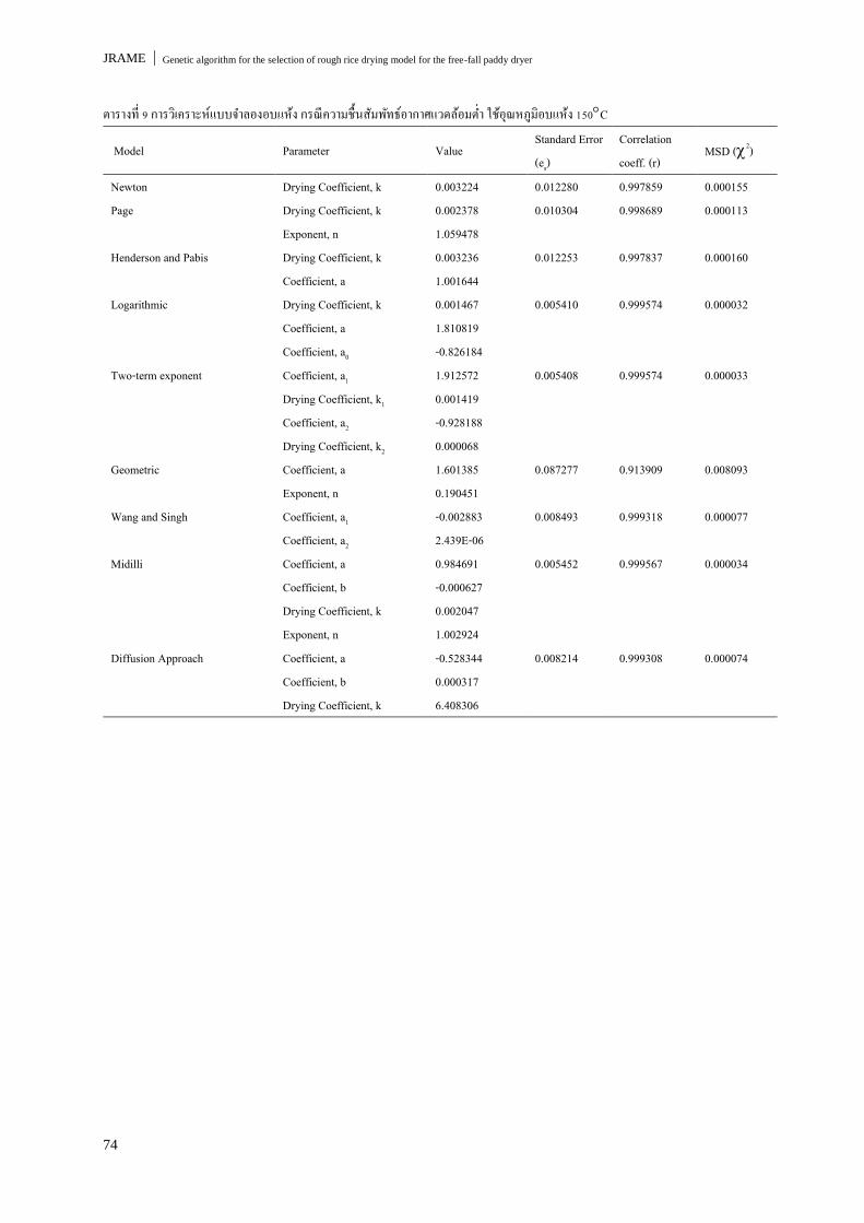
JRAME Genetic algorithm for the selection of rough rice drying model for the free-fall paddy dryer
74
ตารางท 9 การวเคราะหแบบจ าลองอบแหง กรณความชนสมพทธอากาศแวดลอมต า ใชอณหภมอบแหง 150C
Model Parameter Value Standard Error (es)
Correlation coeff. (r)
MSD (2)
Newton Drying Coefficient, k 0.003224 0.012280 0.997859 0.000155 Page Drying Coefficient, k 0.002378 0.010304 0.998689 0.000113
Exponent, n 1.059478 Henderson and Pabis Drying Coefficient, k 0.003236 0.012253 0.997837 0.000160
Coefficient, a 1.001644 Logarithmic Drying Coefficient, k 0.001467 0.005410 0.999574 0.000032
Coefficient, a 1.810819 Coefficient, a0 -0.826184
Two-term exponent Coefficient, a1 1.912572 0.005408 0.999574 0.000033 Drying Coefficient, k1 0.001419 Coefficient, a2 -0.928188 Drying Coefficient, k2 0.000068
Geometric Coefficient, a 1.601385 0.087277 0.913909 0.008093 Exponent, n 0.190451
Wang and Singh Coefficient, a1 -0.002883 0.008493 0.999318 0.000077 Coefficient, a2 2.439E-06
Midilli Coefficient, a 0.984691 0.005452 0.999567 0.000034 Coefficient, b -0.000627 Drying Coefficient, k 0.002047 Exponent, n 1.002924
Diffusion Approach Coefficient, a -0.528344 0.008214 0.999308 0.000074 Coefficient, b 0.000317 Drying Coefficient, k 6.408306
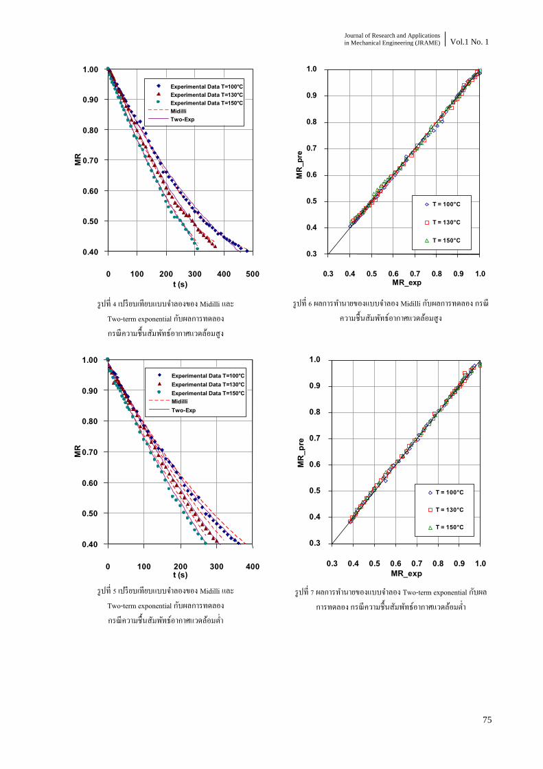
Journal of Research and Applications
in Mechanical Engineering (JRAME) Vol.1 No. 1
75
รปท 4 เปรยบเทยบแบบจ าลองของ Midilli และ
Two-term exponential กบผลการทดลอง กรณความชนสมพทธอากาศแวดลอมสง
รปท 5 เปรยบเทยบแบบจ าลองของ Midilli และ
Two-term exponential กบผลการทดลอง กรณความชนสมพทธอากาศแวดลอมต า
รปท 6 ผลการท านายของแบบจ าลอง Midilli กบผลการทดลอง กรณ
ความชนสมพทธอากาศแวดลอมสง
รปท 7 ผลการท านายของแบบจ าลอง Two-term exponential กบผล
การทดลอง กรณความชนสมพทธอากาศแวดลอมต า
0.40
0.50
0.60
0.70
0.80
0.90
1.00
0 100 200 300 400 500t (s)
MRExperimental Data T=100°CExperimental Data T=130°CExperimental Data T=150°CMidilliTwo-Exp
0.40
0.50
0.60
0.70
0.80
0.90
1.00
0 100 200 300 400t (s)
MR
Experimental Data T=100°CExperimental Data T=130°CExperimental Data T=150°CMidilliTwo-Exp
0.3
0.4
0.5
0.6
0.7
0.8
0.9
1.0
0.3 0.4 0.5 0.6 0.7 0.8 0.9 1.0
MR_
pre
MR_exp
T = 100°C
T = 130°C
T = 150°C
0.3
0.4
0.5
0.6
0.7
0.8
0.9
1.0
0.3 0.4 0.5 0.6 0.7 0.8 0.9 1.0
MR_p
re
MR_exp
T = 100°C
T = 130°C
T = 150°C
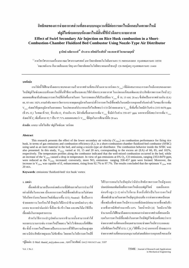
*ผตดตอ: E-Mail: [email protected] , เบอรโทรศพท: (662) 9883655 ext. 3107
Vol. 1 No.1 TSME | Journal of Research and Applications in Mechanical Engineering
อทธพลของการจายอากาศสวนทสองแบบหมนวนทมตอการเผาไหมแกลบในเตาเผาไหม ฟลอไดซเบดแบบหองเผาไหมสนทใชหวฉดกระจายอากาศ
Effect of Swirl Secondary Air Injection on Rice Husk combustion in a Short-
Combustion-Chamber Fluidized Bed Combustor Using Nozzle-Type Air Distributor
ฐานตย เมธยานนท1 ประสาน สถตยเรองศกด2 และสมชาต โสภณรณฤทธ3
1,2 ภาควชาวศวกรรมเครองกล คณะวศวกรรมศาสตร มหาวทยาลยเทคโนโลยมหานคร 51 เขตหนองจอก กรงเทพมหานคร 10530 3คณะพลงงาน สงแวดลอมและวสด มหาวทยาลยเทคโนโลยพระจอมเกลาธนบร 126 เขตทงคร กรงเทพมหานคร 10400
บทคดยอ
งานวจยนไดศกษาถงผลกระทบของความเรวอากาศสวนทสองใตวงแหวนวอรเทค (V2,low) ทมตอสมรรถนะการเผาไหมแกลบของเตาเผาไหมฟลอไดซเบดแบบหองเผาไหมสนทใชทรายเปนเบดและใชหวฉดกระจายอากาศ ในแงของแกสมลพษและประสทธภาพการเผาไหม (Ec) ตลอดจนศกษาถงลกษณะการเผาไหมทเกดขนภายในเตา ในการทดลองไดปรบเปลยน V2,low ท 10, 15 และ 20 m/s ซงคดเปนอากาศสวนเกน (EA) 66, 85 และ 102% ตามล าดบ ผลการวดการกระจายอณหภมภายในเตาบงชวาการเผาไหมเชอเพลงในเบดมการคลกเคลากนอยางด ในขณะทการเพม V2,low สงผลใหอณหภมภายในเตาลดลง ในแงขององคประกอบแกสไอเสยพบวา CO มคาลดลงตาม V2,low ทเพมขนโดยมคาในชวง 2353-8470 ppm (ท 6% O2) ในขณะท NOx ทระดบ O2 สวนเกน 6% มคาเพมขนตามการเพม V2,low ซงมคาในชวง 358-457 ppm นอกจากนยงพบวาการเพม V2,low สงผลให Ec เพมขนจาก 92.7 เปน 97.71% ตลอดจนพบวา V2,low ทดสดในการศกษานคอ 20 m/s
ค าหลก: แกลบ/ แกสไอเสย/ ฟลอไดซเบด/ วอรเทค
Abstract
This research presents the effect of the lower secondary air velocity (V2,low) on combustion performance for firing rice
husk, in terms of gas emissions and combustion efficiency (Ec), in a short-combustion-chamber fluidized-bed combustor (SFBC)
using sand as an inert material in the bed, and using a nozzle-type air distributor. The combustion behavior inside the SFBC was
also presented. In this study, V2,low varied at 10, 15 and 20 m/s, corresponding to the excess air (EA) of 66, 85, and 102%,
respectively. The temperature profiles along the combustor indicated that the well-mixed combustion occurred in the bed, while
an increase of the V2,low caused a drop in temperature. In view of gas emissions at 6% O2, CO emissions, ranging 2353-8470 ppm,
were reduced as the V2,low increased; conversely, more NOx emissions ranging 358-457 ppm were formed. Moreover, the
increase in V2,low was capable of Ec enhancement, rising from 92.7% to 97.7%. The results concluded that the optimum V2,low was
20 m/s.
Keywords: emissions/ fluidized-bed/ rice husk/ vortex
1. บทน า เชอเพลงชวมวลเปนแหลงพลงงานทมศกยภาพในการน ามาใช
อยางย งยนในอนาคต เนองจากการเผาไหมเชอเพลงชวมวลไมสงผลใหแกสคารบอนไดออกไซดเพมมากขน (CO2-Neutral) ซงเปนการชวยลดสภาวะโลกรอนได ปจจบนไดมกรน าชวมวลชนดตางๆ เชน แกลบ ทะลายปาลมเปลา ขเลอย ซง-ขาวโพด และเศษไมมาใชเปนเชอเพลงในภาคอตสาหกรรม
ส าหรบวธการแปรรปพลงงานจากชวมวลน นสามารถท าไดหลายกระบวนการเชน การเผาไหมโดยตรง ไพโรไรซสและแกสซฟเค ชน ทงน การเผาไหมโดยตรงเปนกระบวนการทไดรบความนยมสงสดเพราะมประสทธภาพสงและไมซบซอน โดยเทคโนโลยการเผาไหมท
ไดรบการยอมรบในปจจบนวามประสทธภาพการเผาไหมสงและปลดปลอยมลพษนอยคอการเผาไหมแบบฟลอไดซ เบดเนองจาก คอนขางสง [1-3] อยางไรกตาม สงหนงทจ าเปนในการเผาไหมเชอเพลงชวมวลในเตาเผาไหมทกรปแบบคอ การจายอากาศเหนอเบด เชอเพลงเพอชวยเผาไหมสารระเหยทปลดปลอยมาจากเชอเพลงชวมวลซงอาจมสดสวนมากถง 60% โดยน าหนก [4] โดยมงานวจยจ านวนหนงไดศกษาถงผลกระทบของการจายอากาศสวนทสองเหนอ เบดในการเผาไหมเชอเพลงในเตาเผาไหมฟลอไดซเบดซงพบวาการจายอากาศสวนทสองเหนอเบดสามารถจะชวยเผาไหมสารระเหยและ แกสทยงเผาไหมได (CO, CxHy) ไดดขน [5-6] นอกจากน ลกษณะการจายอากาศสวนทสองแบบหมนวนยงสงผลดตอการคลกเคลาของแกส

JRAME Effect of Swirl Secondary Air Injection on Rice Husk combustion in a Short-
Combustion-Chamber Fluidized Bed Combustor Using Nozzle-Type Air Distributor
78
และอนภาคเชอเพลงภายในเตาซงจะสงผลดตอการเผาไหมทดขนอกดวย
งานวจยทผานมาของคณะผวจยทไดศกษาการเผาไหมแกลบในเตาเผาไหมฟลอไดซเบดแบบหองเผาไหมสน (SFBC) ซงไมใชวสดเฉอยเปนเบดและตดตงใบกวนภายในเบดเพอปองกนการเกาะตวของเชอเพลง [7] ซงผลการศกษาพบวาสามารถเผาไหมเชอเพลงแกลบไดอยางมประสทธภาพและปลดปลอยแกสมลพษอยในเกณฑมาตรฐาน แตทงน การไมผสมวสดเฉอยในเบดของเตา SFBC สงผลใหเกดขดจ ากดในการน าเตาเผาไหมตวนไปประยกตใชกบเชอเพลงชนดอนทไมสามารถท าใหเกดสภาวะฟลอไดซเซชนหากปราศจากอนภาคเบด จงไดปรบเปลยนการศกษามาเปนการใชทรายเปนเบดปรมาณ 6 kg ซงจ าเปนตองท าการศกษาผลกระทบของปจจยตางๆ ทสงผลตอการเผาไหมในเตาเผาไหม SFBC
วตถประสงคของงานวจยนคอการศกษาผลกระทบความเรวอากาศสวนทสองทจายใตวงแหวนแบบหมนวนทมตอสมรรถนะการเผาไหมแกลบของเตาเผาไหม SFBC ทใชทรายเปนเบด ซงจะพจารณาถงลกษณะการเผาไหม องคประกอบของแกสไอเสยและประสทธภาพการเผาไหม โดยในทกเงอนไขการทดลองจะปรบอตราการปอนเชอเพลงและความเรวอากาศในสวนอนๆ ไวคงทแตจะปรบเปลยนเพยงความเรวของอากาศสวนทสองใตวงแหวนวอรเทคเทานน
2. อปกรณและวธการทดลอง 2.1 เตาเผาไหมฟลอไดซเบดแบบหองเผาไหมสน
เตาเผาไหมฟลอไดซเบดแบบหองเผาไหมสนทใชในการทดลองนนมไดอะแกรมดงแสดงในรปท 1 ลกษณะของเตาเผาไหมสามารถแบงออกเปนสองสวนดงรปท 2 คอ 1) เตาเผาไหมทเปนทรงกระบอกทมขนาดเสนผานศนยกลางภายในเตาเทากบ 500 mm และสง 1525 mm และ 2) สวนกรวยซงมขนาดเสนผานศนยกลางยอดตดกรวย 300 mm สง 500 mm ซงถกออกแบบส าหรบรองรบอนภาคเบดและเชอเพลงทยงเผาไหมไมหมด ผนงเตาดานในกอดวยอฐและฉาบดวยซเมนตทนไฟหนา 125 mm ในสวนของตวเตาเผาทเปนทรง กระบอกไดมการตดตงวงแหวนวอร-เทคทระดบความสง1380 mm (เหนอแผนกระจายอากาศ) ซงมขนาดเสนผานศนยกลางรวงแหวนเทากบ 300 mm เพอดกอนภาคทยงเผาไหมไมหมดทอาจหลดลอยขนเมอเกดการฟ งกระจายของเชอเพลง
การจายอากาศเขาเตาเผาไหมมดวยกนสามสวนดงนคอ 1) อากาศ
สวนทหนงซงเปนอากาศทกอใหเกดฟลอไดเซชน 2) อากาศสวนทสองเปนอากาศทชวยในการเผาไหมและชวยในการดกจบอนภาคทยงเผาไหมไมหมดซงมการจายทสองระดบความสงคอระดบเหนอวงแหวนวอรเทค (vortex ring) ทระดบ1490 mm ซงถกจายในลกษณะสมผสกบผนงเตาเผาไหมจ านวน 1 ทอ และระดบใตวงแหวนวอร เทคซงจายในลกษณะท ามมกบเสนสมผสผนงเตาท 65 องศา จ านวน 4 ทอ (ระดบ 1030 mm) ซงจะกอใหเกดวงแหวนอากาศทมขนาดเสนผานศนยกลาง 200 mm และ 3) อากาศสวนทสามเปนอากาศซงจายเพอใชเผาไหมและปองกนการลกลามของไฟทจะเขาไปยงถงพกปอนแกลบ
นอกจากน ในการทดลองจะใชทรายขนาด 300 ไมครอนเปนเบดปรมาณ 6 kg และใชตวกระจายอากาศแบบหวฉดซงมขนาดเสนผานศนยกลาง 37 mm สง 55 mm จ านวน 8 หวทถกตดตงบนแผนกระจายอากาศ ในการปอนเชอเพลงเขาสเตาเผาไหมจะใชระบบสกรปอน (Screw feeder) เขาในเบดโดยตรงทระดบความสง 650 mm เหนอแผนกระจายอากาศ
2.2 องคประกอบของเชอเพลงทใชในการทดลอง เชอเพลงทเลอกใชในงานวจยนคอแกลบซงมองคประกอบของเชอเพลงดงแสดงในตารางท 1 ตารางท 1 องคประกอบของเชอเพลงแกลบ (as received)
Proximate analysis (wt.%) Fixed carbon 20.1 Volatile matter 55.6 Moisture 10.3 Ash 14.0
Ultimate analysis (wt.%) Carbon 38.0 Hydrogen 4.55 Oxygen 32.4 Nitrogen 0.69 Sulphur 0.06 Moisture 10.3 Ash 14.0
Higher heating value (MJ/kg) 14.98
รปท 1 ไดอะแกรมเตาเผาไหมฟลอไดซเบดแบบหองเผาไหมสนทใชในการทดลอง

Journal of Research and Applications
in Mechanical Engineering (JRAME) Vol.1 No. 1
79
รปท 2 ขนาดเตาและต าแหนงการวดอณหภมและแกสไอเสยของเตาเผาไหมฟลอไดซเบดแบบหองเผาไหมสน 2.3 การวดและขนตอนการทดลอง การวดปรมาณอากาศทใชในการทดลองของงานวจยนไดใชเวนจรทท าการสอบเทยบแลวรวมกบเซนเซอรวดความดนแตกตางซงมความคลาดเคลอน 3% ของยานการวด เปนอปกรณในการวดอตราการไหลของอากาศ การควบคมอตราการปอนเชอเพลงจะใชอนเวอรเตอรควบคมความเรวรอบมอเตอรทใชขบสกรปอนเชอเพลง สวนการวดอณหภมในการทดลองทระดบความสงตางๆ เหนอแผนกระจายอากาศคอ 640, 960, 1280 และ 1630 mm ตลอดจนททอทางออกเตาจะใชเทอรโมคบเปลชนด K คกบอปกรณแสดงผลซงมความละเอยด 1oC สวนการวดองคประกอบแกสเผาไหมททอทางออกเตานนไดใชเครองวเคราะหแกสเสย Testo 350XL ซงสามารถวดแกส O2, CO, และ NOx, สวน CO2 ทแสดงนนไดมาจากการค านวณยอนกลบจากปรมาณ O2 ของเครองวด สวนประสทธภาพการเผาไหมของเตานนหาไดจากการวเคราะหปรมาณคารบอนทไมเผาไหมภายในเถาทดกไดจากไซโคลนโดยใชเครองวเคราะหองคประกอบธาต LECO CHNS 932 รวมกบปรมาณ CO ทวดได ขนตอนการทดลองเรมจากการปรบความเรวอากาศสวนตางๆ ของแตละเงอนไขการทดลอง ดงตารางท 2 จากนนท าการจดเตาเผา ไหม โดยจะเรมใชแกลบเปนเชอเพลงเพออนใหเตาอณหภมสงขนประมาณ 700 -800C แลวจงเรมปอนทรายเขาสเตาเผาไหมใหไดปรมาณ 6 kg หลงจากนนจงท าการปรบอตราการปอนเชอเพลงดวยอนเวอรเตอรใหไดตามเงอนไขการทดลอง เมอสภาวะการท างานของเตาเผาไหมเขาสสภาวะคงตว (Steady) ซงใชเวลาประมาณ 60-90 นาทแลวจงเรมบนทกคาตาง ๆ ดงนคอ อณหภมภายในเตาทระดบความสงตางๆ (ดงรปท 2) องคประกอบแกสไอเสยททอทางออกเตา และปรมาณเถาทดกไดจากไซโคลน (เกบทก 30 นาท เปนเวลา 10 นาท) เพอน าไปวเคราะหหาคารบอนทยงไมเผาไหม โดยขอมลทไดจะถกน าไปค านวณหาประสทธภาพการเผาไหม (Ec)ไดตามสมการท (1) [2, 7-9]
%100)--(
Ec
FEfgEaEFE
(1)
โดย EF = ปรมาณความรอนทไดจากเชอเพลงทปอนเขาเตาเผาไหม (MJ/kg) Ea = ปรมาณความรอนทสญเสยไปกบคารบอนทไมเผาไหมในเถา
(MJ/kg)
Efg= ปรมาณความรอนทสญเสยไปกบแกสคารบอนมอนออกไซด
(CO) ในแกสไอเสยซงค านวณไดจากปรมาณ COคาความรอนของ
CO (MJ/kg)
ตารางท 2 เงอนไขการทดลองผลกระทบของความเรวอากาศสวนทสองใตวงแหวนวอรเทค
Testing conditions Run number
1 2 3
Fluidizing air velocity (m/s) 1 1 1 Mass fraction (-) 0.570 0.521 0.494 Lower 2nd air velocity (m/s) 10 15 20 Mass fraction (-) 0.207 0.276 0.314 Upper 2nd air velocity (m/s) 15 15 15 Mass fraction (-) 0.076 0.069 0.065 Tertiary air velocity (m/s) 4 4 4 Mass fraction (-) 0.147 0.134 0.127 Excess air (%) 66 85 102 Rice husk feed rate (kg/h) 65 65 65

JRAME Effect of Swirl Secondary Air Injection on Rice Husk combustion in a Short-
Combustion-Chamber Fluidized Bed Combustor Using Nozzle-Type Air Distributor
80
3. ผลการทดลองและวจารณ จากการทดลองศกษาผลกระทบของความเรวอากาศสวนทสองใตวงแหวนวอคเทค (V2,low) ทจายแบบหมนวนเพอชวยในการเผาไหมแกลบในเตาเผาไหมฟลอไดซเบดแบบหองเผาไหมสน (SFBC) ซงใชทรายเปนเบดปรมาณ 6 kg และใชตวกระจายอากาศแบบหวฉด โดยพจารณาถงลกษณะการ เผาไหมท เ กด ขนภายในเตาจากการเปลยนแปลงอณหภมในแตละระดบความสง ตลอดจนพจารณาถงสมรรถนะของการเผาไหมในแงของประสทธภาพการเผาไหมและองคประกอบแกสไอเสยททางออกเตาซงสามารถแสดงผลไดดงน
3.1 การกระจายอณหภมภายในเตา รปท 4 แสดงการกระจายอณหภมแนวกงกลางเตาทระดบตางๆ ในแตละเงอนไขการจายอากาศสวนทสองแบบหมนวนเพอชวยเผาไหมแกลบทต าแหนงใตวงแหวนวอรเทคดวยความเรว 10, 15 และ 20 m/s โดยพบวาอณหภมเบดทระดบ 640 mm และ 960 mm เหนอแผนกระจายอากาศ ในทกเงอนไขมคาใกลเคยงกนในชวงประมาณ 945oC (ทระดบ 640 mm) และ 955-971oC (ทระดบ 960 mm) ซงแสดงใหเหนถงการคลกเคลาทด (well mixing) ภายในเบด นอกจากนยงพบวาการเผาไหมจะเกดขนอยางตอเนองจนถงทอทางออกของเตาเผาไหม ทงนเปนทนาสงเกตวาในกรณการจายอากาศสวนทสองใต วงแหวนวอรเทคดวยความเรว 10 m/s สงผลใหอณหภมทระดบ 1280 mm มคาสงขนอยางชดเจน ซงสามารถอธบายไดวา เนองจากกรณนใชปรมาณอากาศสวนเกนทต าสด (EA=66%) จงท าใหปรมาณแกสคารบอนมอนออกไซด (CO) เกดขนขณะเผาไหมเชอเพลงภายในเบดมปรมาณมาก ซง CO นจะลอยขนมาเผาไหมกบอากาศสวนทสองใตวงแหวนวอรเทค (สดสวนมวล 0.20) อยางรนแรง ในขณะทเงอนไข V2,low เทากบ 15 และ 20 m/s (EA=85 และ 102% ตามล าดบ) นนอณหภมทระดบความสงเดยวกนนเพมขนไมมากนก เนองจากมวลอากาศสวนทสองใตวงแหวนวอรเทคซงถกจายเขาไปในเตาของท งสองเงอนไขมสดสวนมวลอากาศทสง (0.28-0.31) โดยอณหภมทระดบความสง 1280 mm นมคาลดลงตามปรมาณอากาศทเพมขนคอ 1067, 990 และ 960oC ตามล าดบ
รปท 3 การกระจายอณหภมแนวกงกลางเตาเผาไหม
ส าหรบระดบเหนอวงแหวนวอรเทค (1630 mm) พบวาอณหภมในทกเงอนไขมคาเพมขนเมอเทยบกบระดบใตวงแหวนวอรเทค (1000-1100oC) ซงบงบอกไดถงการเผาไหมทเกดขนอยางตอเนองของ CO ทหลดลอยขนมาเผาไหมกบอากาศสวนทสองเหนอวงแหวนวอรเทค สวนทระดบความสงต งแต 1630 mm จนถงทอทางออกเตาอณหภมในทกเงอนมการเปลยนแปลงเพยงเลกนอย แสดงใหเหนวาการเผาไหมเกดขนนอยลงทชวงระดบความสงดงกลาว โดยอณหภมทางออกทเงอนไขความเรวอากาศสวนทสองใตวงแหวนวอรเทคท 10, 15 และ 20 m/s คอ 1090, 1018 และ 978oC ตามล าดบ
3.2 องคประกอบแกสเสยททางออกเตา ผลกระทบของความเรวอากาศสวนทสองใต วงแหวนวอรเทค (V2,low) ทมตอแกสไอเสยททางออกเตาคอ ออกซเจน (O2) คารบอนมอนออกไซด (CO) และไนโตรเจนออกไซด (NOx) สามารถแสดงไดดงรปท 4 โดยรปท 4(ก) แสดงใหเหนวาปรมาณ O2 มคาเพมขนตามการเพมขนของความเรวอากาศสวนทสอง (อากาศสวนเกนทเพมขน) จาก 7.08% เปน 10.07% สวน CO ททางออกเตาภายใต O2 สวนเกน 6% พบวามคาลดลงตาม V2,low ทเพมขนอยางชดเจนดงรปท 4(ข) โดยมคาลดลงจาก 8470 ppm เหลอ 2353 ppm เนองจากอากาศสวนทสองนมการจายแบบหมนวนทท าใหเกดเปนวงแหวนอากาศซงสามารถชวยให CO ทเกดขนอยางมากในเบดถกท าปฏกรยาไดดขน โดยความปนปวนของอากาศในต าแหนงนจะมคาเพมขนตามความเรวอากาศจงเปนเหตผลใหปรมาณ CO มคาลดลง [6] อยางไรกตามปรมาณ CO ทวดไดในทกเงอนไขการทดลองมคาสงกวาคามาตรฐานซงมคาเพยง 740 ppm (ท 6% O2) ทงน อาจเปนผลของความเรวอากาศทกอใหเกดฟลอไดเซชนทใชในการศกษามคาสงเกนไป (1 m/s) จงท าใหความเรวแกสภายในเตามคาสงซงเปนผลใหระยะเวลาการเผาไหมในเตาส นเกนไป ในแงของ NOx พบวามคาเพมขนอยางมากตามการเพมขนของความเรวอากาศสวนทสองใตวงแหวนวอรเทค โดยเฉพาะกรณทการเพมความเรวจาก 10 m/s เปน 15 m/s (EA จาก 66% เปน 85%) ซงเพมจาก 358 เปน 457 ppm ท 6% O2 ดงรปท 4(ค) ผลทเกดขนนอธบายไดจากสารระเหยของแกลบซงมกอยในรป NH3 [4, 8-9] ทปลดปลอยมาจากเชอเพลงมาเผาไหมบรเวณทมการจายอากาศสวนทสองใตวงแหวนวอร-เทคตามสมการ (2) และ (3) [8-10]
NONHNHOOHO
iOHO
,,,
32 (2)
NONHOchar
2,
3 (3)
จากสมการทงสองแสดงใหเหนวาปรมาณ O2 ทเพมขนจะสงผลโดยตรงตอการเกดปฏกรยาการกอตวของ NOx ดงนนการเพม V2,low จงเปรยบเสมอนการเพม O2 ในการเขาท าปฏกรยาการเกด NOx มากขน สวนกรณการเพมปรมาณอากาศสวนเกนเปน 102% (V2,low = 20 m/s) ซงพบวา NOx มการเพมขนนอยกวาเงอนไขกอนหนา ซงอาจเปนผลสบเนองมาจากในเงอนไขนใชปรมาณอากาศมากจนสงใหอณหภม
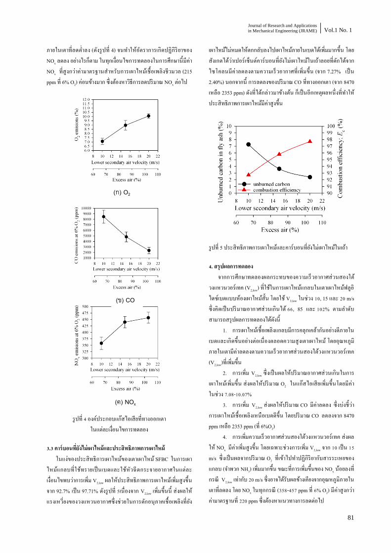
Journal of Research and Applications
in Mechanical Engineering (JRAME) Vol.1 No. 1
81
ภายในเตาทลดต าลง (ดงรปท 4) จนท าใหอตราการเกดปฏกรยาของ NOx ลดลง อยางไรกตาม ในทกเงอนไขการทดลองในการศกษานมคา NOx ทสงกวาคามาตรฐานส าหรบการเผาไหมเชอเพลงชวมวล (215 ppm ท 6% O2) คอนขางมาก ซงตองหาวธการลดปรมาณ NOx ตอไป
รปท 4 องคประกอบแกสไอเสยททางออกเตา ในแตละเงอนไขการทดลอง
3.3 คารบอนทยงไมเผาไหมและประสทธภาพการเผาไหม ในแงของประสทธการเผาไหมของเตาเผาไหม SFBC ในการเผาไหมแกลบทใชทรายเปนเบดและใชหวฉดกระจายอากาศในแตละเงอนไขพบวาการเพม V2,low ผลใหประสทธภาพการเผาไหมเพมสงขนจาก 92.7% เปน 97.71% ดงรปท 5เนองจาก V2,low เพมขนน สงผลใหแรงเหวยงของวงแหวนอากาศซงชวยในการดกอนภาคเชอเพลงทยง
เผาไหมไมหมดใหตกกลบลงไปเผาไหมภายในเบดไดเพมมากขน โดยสงเกตไดวาเปอรเซนตคารบอนทยงไมเผาไหมในเถาลอยทดกไดจากไซโคลนมคาลดลงตามความเรวอากาศทเพมขน (จาก 7.27% เปน 2.40%) นอกจากน การลดลงของปรมาณ CO ททางออกเตา (จาก 8470 เหลอ 2353 ppm) ดงทไดกลาวมาขางตน กเปนอกเหตผลหนงทท าใหประสทธภาพการเผาไหมมคาสงขน
รปท 5 ประสทธภาพการเผาไหมและคารบอนทยงไมเผาไหมในเถา
4. สรปผลการทดลอง จากการศกษาทดลองผลกระทบของความเรวอากาศสวนสองใตวงแหวนวอรเทค (V2,low) ทใชในการเผาไหมแกลบในเตาเผาไหมฟลอไดซเบดแบบหองเผาไหมสน โดยใช V2,low ในชวง 10, 15 และ 20 m/sซงคดเปนปรมาณอากาศสวนเกนได 66, 85 และ 102% ตามล าดบ สามารถสรปผลการทดลองไดดงน
1. การเผาไหมเชอเพลงแกลบมการคลกเคลากนอยางดภายในเบดและเกดขนอยางตอเนองตลอดความสงเตาเผาไหม โดยอณหภมภายในเตามคาลดลงตามความเรวอากาศสวนสองใตวงแหวนวอรเทค (V2,low)ทเพมขน
2. การเพม V2,low ซงเปนผลใหปรมาณอากาศสวนเกนในการเผาไหมเพมขน สงผลใหปรมาณ O2 ในแกสไอเสยเพมขนโดยมคาในชวง 7.08-10.07%
3. การเพม V2,low สงผลใหปรมาณ CO มคาลดลง ซงบงชวาการเผาไหมเชอเพลงเหนอเบดดขน โดยปรมาณ CO ลดลงจาก 8470 ppm เหลอ 2353 ppm (ท 6%O2)
4. การเพมความเรวอากาศสวนสองใตวงแหวนวอรเทค สงผลให NOx มคาเพมสงขน โดยเฉพาะชวงการเพม V2,low จาก 10 เปน 15 m/s ซงเปนผลจากปรมาณ O2 ทเขาไปท าปฏกรยากบสารระเหยของแกลบ (จ าพวก NH3) เพมมากขน ขณะทการเพมขนของ NOx นอยลงทกรณ V2,low เทากบ 20 m/s ซงอาจไดรบผลขางเคยงจากอณหภมภายในเตาทลดลง โดย NOx ในทกกรณ (358-457 ppm ท 6% O2) มคาสงกวาคามาตรฐานท 220 ppm ซงตองหาแนวทางการลดตอไป
(ก) O2
(ข) CO
(ค) NOx
JRAME Effect of Swirl Secondary Air Injection on Rice Husk combustion in a Short-
Combustion-Chamber Fluidized Bed Combustor Using Nozzle-Type Air Distributor
82
5. การเพม V2,low สงผลใหการคลกเคลาของอากาศและอนภาคเชอเพลงตลอดจนแกสทยงเผาไหมไมสมบรณไดดขน ซงดไดจากปรมาณ CO และคารบอนทไมเผาไหมทลดลง เปนผลใหประสทธภาพการเผาไหมมคาเพมขนจาก 92.7 เปน 97.75% โดยเงอนไขความเรว V2,low ทดสดในการศกษาคอ 20 m/s
5. กตตกรรมประกาศ ขอขอบคณส านกงานกองทนสนบสนนการวจย (สกว .) ส านกงานคณะกรรมการการอดมศกษา (สกอ.) ทใหการสนบสนนทนวจย
6. เอกสารอางอง [1] Natarajan, E., Nordin, A., Rao, A.N., 1998. Overview of combustion and gasification of rice husk in fluidized bed reactors.
Biomass Bioenergy, Vol. 14, pp. 533-546.
[2] Armesto, L., Bahillo, A., Veijonen, K., Cabanillas, A., Otero, J., 2002. Combustion behaviour of rice husk in a bubbling fluidised
bed. Biomass Bioenergy, Vol. 23, pp.171-179.
[3] Fang, M., Yang, L., Chen, G., Shi, Z., Luo, Z., Cen, K., 2004. Experimental study on rice husk combustion in a circulating
fluidized bed. Fuel Process Technol, Vol. 85, pp. 1273-1282.
[4] Werther, J., Saenger, M., Hartge, EU., Ogada, T., Siagi, Z., 2000. Combustion of agricultural residues. Prog Energy Combust
Sci, Vol. 26, pp. 1-27.
[5] Armesto, L., Bahillo, A., Cabanillas, A., Veijonen, K., Otero, J., Plumed, A., Salvador, L., 2003. Co-combustion of coal and olive oil
industry residues in fluidised bed. Fuel, Vol. 82, pp. 993-1000.
[6] Varol, M., Atimtay, AT., 2007. Combustion of olive cake and coal in a bubbling fluidized bed with secondary air injection. Fuel,
Vol. 86, pp. 1430-1438.
[7] Madhiyanon, T., Sathitruangsak, P., Soponronnarit, S., 2010. Combustion behavior of rice-husk in a short-combustion-chamber
fluidized -bed combustor (SFBC). Applied Thermal Engineering,
Vol. 30, pp. 347-353. [8] Sathitruangsak, S., Madhiyanon, M., Soponronnarit, S., 2009.
Rice husk co-firing with coal in a short-combustion-chamber
fluidized-bed combustor (SFBC). Fuel, Vol. 88, pp.1394-1402. [9] Madhiyanon, M., Sathitruangsak, S., Soponronnarit, S., 2009.
Co-combustion of rice husk with coal in a cyclonic fluidized-bed
combustor (-FBC). Fuel, Vol. 88, pp. 132-138. [10] Zevenhoven, R., Kilpinen, P., 2002. Control of pollutants in
flue gases and fuel gases. 2nd edition, Finland, Espoo/Turku.

Subscription Form
Journal of Research and Applications in Mechanical Engineering (JRAME)
Date _____________________________
Name :____________________________________________________________________
Address :__________________________________________________________________
___________________________________________________________________
__________________________________________________________________
E-mail : _______________________Tel : __________________ Fax : __________________
A subscription to JRAME is requested for year(s) (250 Baht/year, up to 2 issues per year).
Signature _________________________
(_________________________)
Method of Payment : deposit or transfer money to the following account :
Account name : TSME journal
Savings Account No. 707-249035-6, Siam Commercial Bank Plc., Suranaree
University of Technology Branch.
After completing the money transfer, please confirm your payment by faxing the pay-
in slip and the subscription form to the JRAME Office (Fax. (INTL)-66-44-224613),
or sending a scanned copy by e-mail to [email protected]
Journal of Research and Applications in Mechanical Engineering Office
School of Mechanical Engineering, Institute of Engineering
Suranaree University of Technology,
111 University Avenue, Nakhon Ratchasima 30000, Thailand
Tel. (INTL)-66-44-224410, Fax. (INTL)-66-44-224613
E-mail : [email protected] Website : http://eng.sut.ac.th/me/JRAME

GUIDE FOR AUTHORS
The Journal of Research and Applications in Mechanical Engineering publishes results of research, applications,
ideas and innovations related to mechanical engineering issues. Papers submitted to the journal must be (1)
original (2) substantial (3) of significant importance.
PREPARATION OF MANUSCRIPT
Manuscripts submitted to JRAME must be written in English or Thai and should be formatted in the same form
and style as that of the final journal article. A template for the article’s style can be downloaded from
http://eng.sut.ac.th/me/JRAME
The title should contain the article title, authors' names and affiliations and the address for manuscript
correspondence (including e-mail address, telephone and fax numbers). Following the title is a single paragraph
abstract summarizing the main findings of the paper in less than 150 words. After the abstract a list of up to 6
keywords that will be useful for indexing or searching should be included. The main body of the paper should start
right after the keywords. No identifying information, such as the authors' names or affiliations, may appear
anywhere in the document. Experimental procedure, data and computational methods must be explained in
sufficient detail to permit replication by other researchers.
References
References may be cited in the text by Arabic numerals in brackets, e.g., [1], [2], or by the use of author-date, e.g.
Johnson (2011); the former style is preferred. References cited in the text should be in numeral order but this is not
an absolute requirement. Journal titles may be listed in full; abbreviations are also allowable.
Figures
Figures should be numbered consecutively with Arabic numerals. Lettering on drawings should be professional
quality or generated by high-resolution computer graphics. Illustrations in color can be accepted only if the authors
defray the cost. TIF or EPS files are required for figures.
Tables
Tables should be numbered consecutively with Roman numerals in order of appearance in the text.
SUBMISSION OF MANUSCRIPT
Files should be saved as Word 2003 (.doc) before uploading, to ensure the equations translate properly.
All manuscripts and enquiries should be submitted via email attachment to [email protected].
Manuscripts are accepted for review with the understanding that the same work has not been and will not be
submitted elsewhere, and that its submission for publication has been approved by all of the authors and by the
institution where the work was carried out. Any person cited as a source of personal communications must approve
such citation.
Articles published in JRAME represent the opinions of the author(s) and should not be construed to reflect the
opinions of the Editor(s) and the Publisher. Copyright in the published manuscripts, including the right to
reproduce the article in all forms and media, shall be assigned exclusively to the Publisher.
ISSN 2229-2152