april, 8-12, 2009 p.1 海大陳正宗終身特聘教授 bipolar coordinates, image method and method...
TRANSCRIPT

April, 8-12, 2009 p.1海大陳正宗終身特聘教授
Bipolar coordinates, image method and method of fundamental solutions
Jeng-Tzong Chen
Department of Harbor and River Engineering,National Taiwan Ocean University
15:30-15:50, April 10, 2009
ICCES 09 in Phuket, Thailand
April, 8-12, 2009 p.2海大陳正宗終身特聘教授
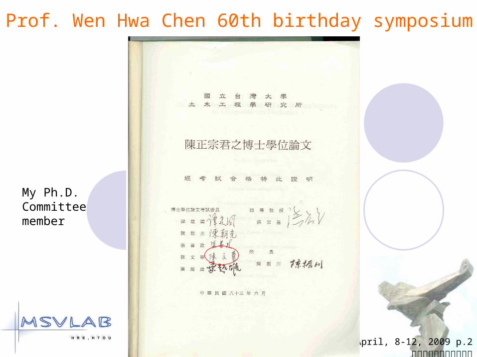
Prof. Wen Hwa Chen 60th birthday symposium
My Ph.D. Committeemember
April 8-12, 2009 p.3海大陳正宗終身特聘教授
Outline
Introduction
Problem statements
Present method MFS (image method) Trefftz method
Equivalence of Trefftz method and MFS
(2-D and 3-D annular cases)
Numerical examples
Conclusions
April 8-12, 2009 p.4海大陳正宗終身特聘教授
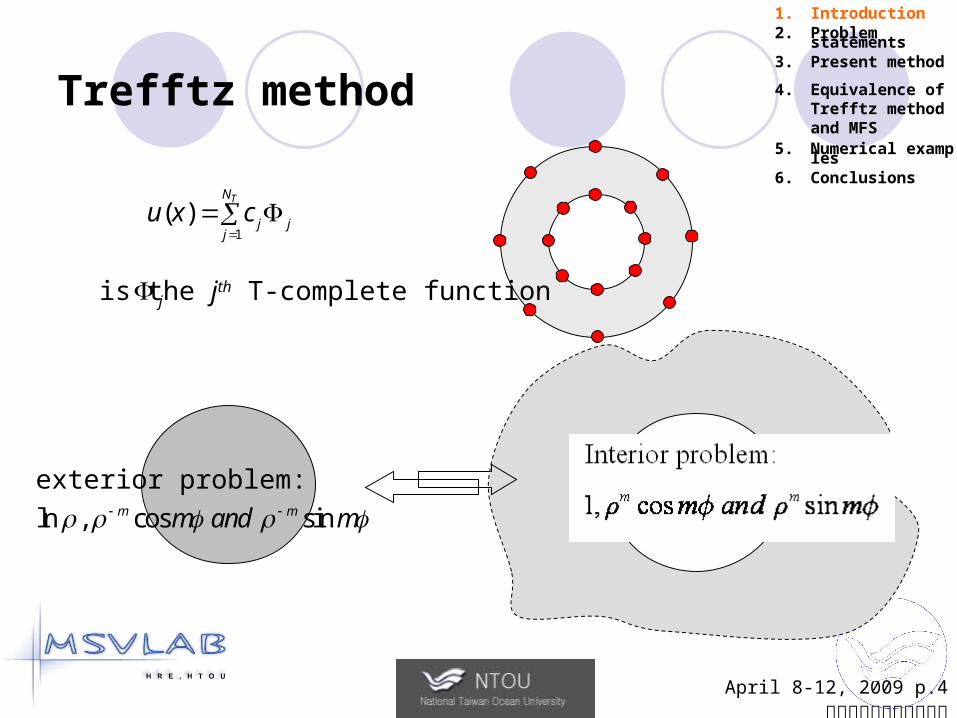
Trefftz method
1. Introduction2. Problem statements3. Present method
4. Equivalence of Trefftz method and MFS
5. Numerical examples6. Conclusions
1( )
TN
j jj
u x c
j is the jth T-complete function
ln , cos sinm mm and m
exterior problem:
April 8-12, 2009 p.5海大陳正宗終身特聘教授
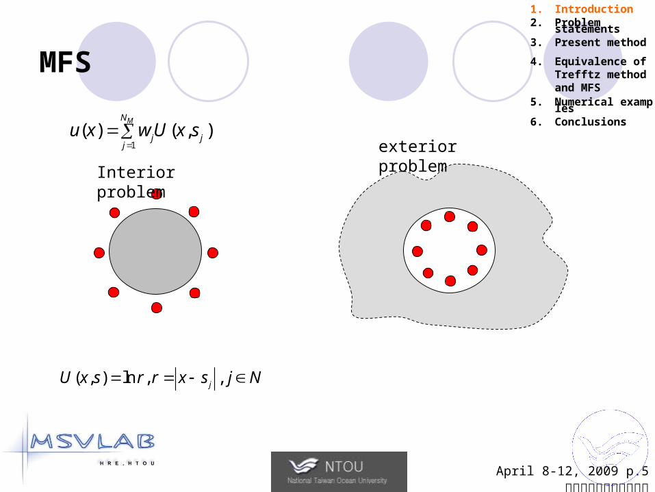
MFS
1. Introduction2. Problem statements3. Present method
4. Equivalence of Trefftz method and MFS
5. Numerical examples6. Conclusions
1( ) ( , )
MN
j jj
u x w U x s
( , ) ln , ,jU x s r r x s j N
Interior problem
exterior problem
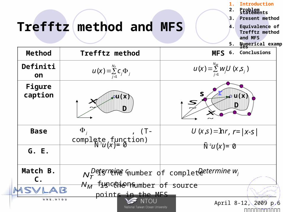
April 8-12, 2009 p.6海大陳正宗終身特聘教授
Trefftz method and MFS
Method Trefftz method MFS
Definition
Figure caption
Base , (T-complete function) , r=|x-s|
G. E.
Match B. C. Determine cj Determine wj
( , ) lnU x s r
1( ) ( , )
MN
j jj
u x w U x s
( )2 0u xÑ = ( )2 0u xÑ =
D
u(x)
~x
s
Du(x)
~x
r
~s
is the number of complete functions TN
MN is the number of source points in the MFS
1. Introduction2. Problem statements3. Present method
4. Equivalence of Trefftz method and MFS
5. Numerical examples6. Conclusions
1( )
TN
j jj
u x c
j
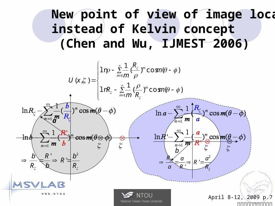
April 8-12, 2009 p.7海大陳正宗終身特聘教授
b
a
New point of view of image locationinstead of Kelvin concept (Chen and Wu, IJMEST 2006)
1
1
)(cos)(1
ln
)(cos)(1
ln
),(
m
m
m
m
mRm
R
mR
mxU
'2
''
R a aR
a R R
'
R
bR
b
R
R
b 2
''
April 8-12, 2009 p.8海大陳正宗終身特聘教授
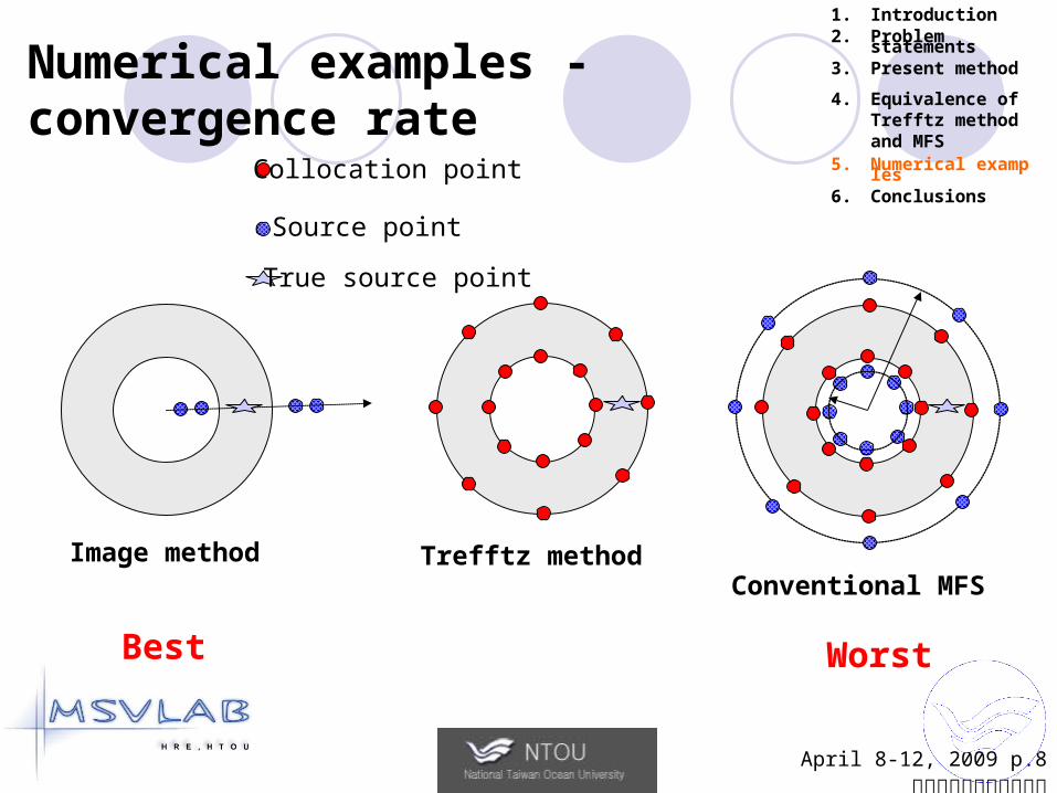
Numerical examples - convergence rate
Image method Trefftz methodConventional MFS
1. Introduction2. Problem statements3. Present method
4. Equivalence of Trefftz method and MFS
5. Numerical examples6. Conclusions
Best Worst
Collocation point
Source point
True source point
April 8-12, 2009 p.9海大陳正宗終身特聘教授
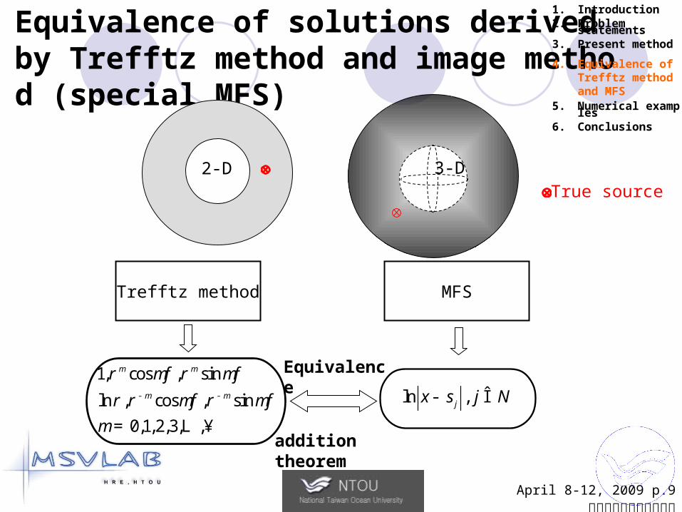
Equivalence of solutions derived by Trefftz method and image method (special MFS)
1. Introduction2. Problem statements3. Present method
4. Equivalence of Trefftz method and MFS
5. Numerical examples6. Conclusions
Trefftz method MFS
1, cos , sin
ln , cos , sin
0,1,2,3, ,
m m
m m
m m
m m
m
r f r f
r r f r f- -
= ¥L
ln ,jx s j N- Î
Equivalence
addition theorem
2-D 3-DTrue source
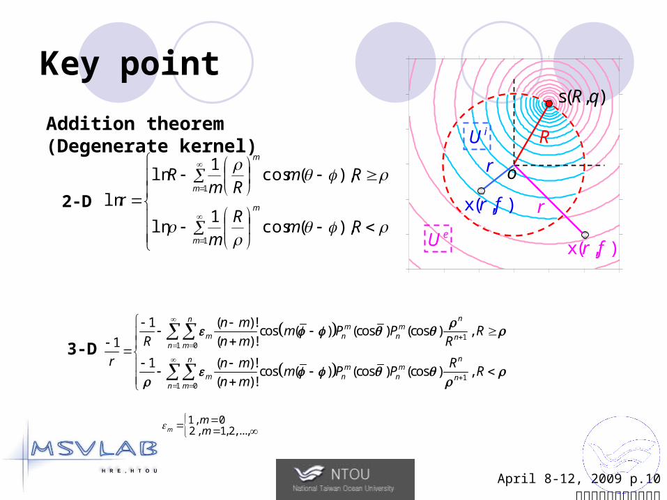
April 8-12, 2009 p.10海大陳正宗終身特聘教授
Key point
Addition theorem (Degenerate kernel)
2-D
RmR
m
RmRm
R
rm
m
m
m
),(cos1
ln
),(cos1
ln
ln
1
1
3-D
11 0
11 0
1 ( )!cos ( ) (cos ) (cos ) ,
( )!1
1 ( )!cos ( ) (cos ) (cos ) ,
( )!
nnm m
m n n nn m
nnm m
m n n nn m
n mm P P R
R n m R
r n m Rm P P R
n m
1, 02 , 1,2,...,m
mm
s( , )R q
R
r
rx( , )r f
x( , )r f
o
iU
eU
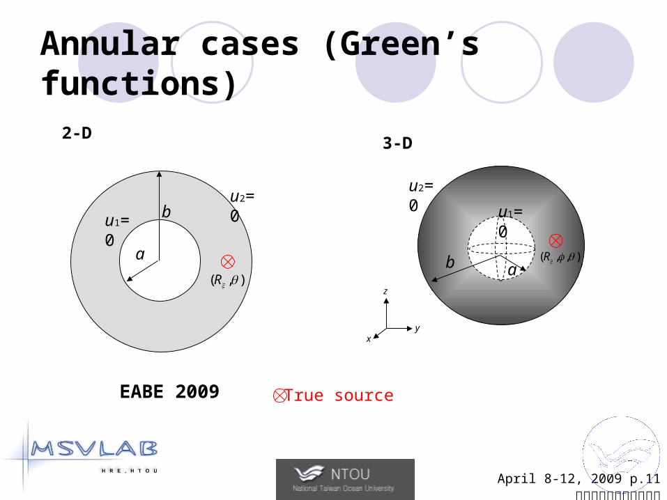
April 8-12, 2009 p.11海大陳正宗終身特聘教授
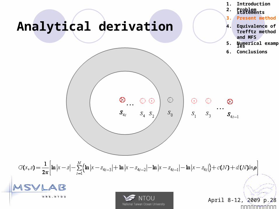
Annular cases (Green’s functions)
2-D
EABE 2009
xy
z
3-D
a
b
ab ),,( R
),( R
u1=0 u1=0u2=0
u2=0
True source
April 8-12, 2009 p.12海大陳正宗終身特聘教授
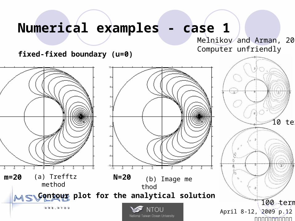
Numerical examples - case 1
(a) Trefftz method (b) Image method
Contour plot for the analytical solution (m=N).
fixed-fixed boundary (u=0)
m=20 N=20
10 terms
100 terms
Melnikov and Arman, 2001Computer unfriendly
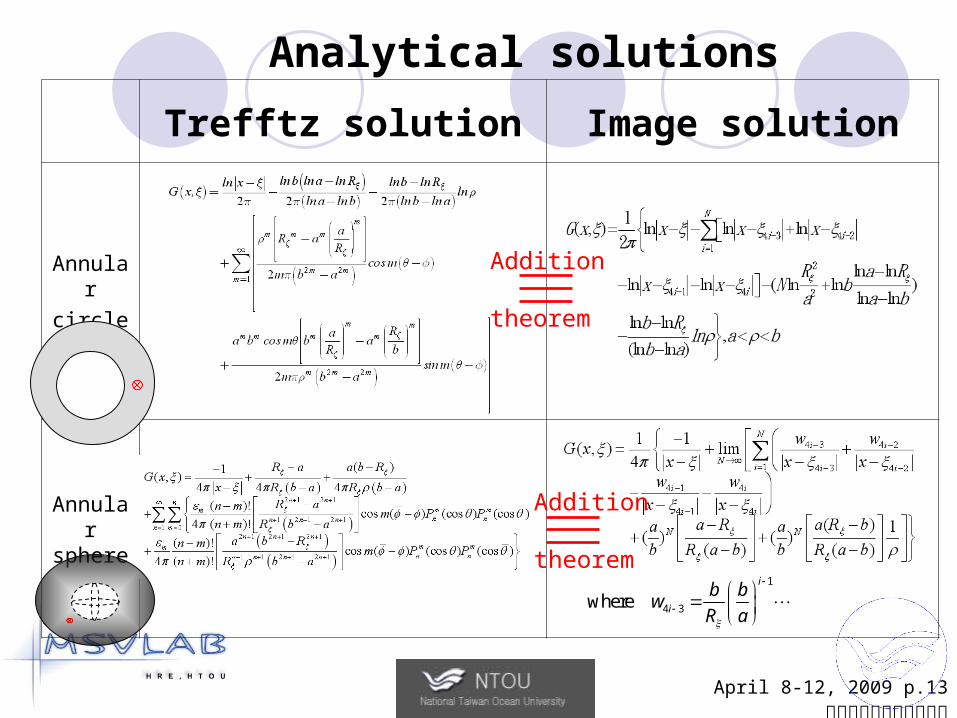
April 8-12, 2009 p.13海大陳正宗終身特聘教授
Trefftz solution Image solution
Annular
circle
Annular sphere
Analytical solutions
1
4 3where i
i
b bw
R a
Addition
theorem
Addition
theorem
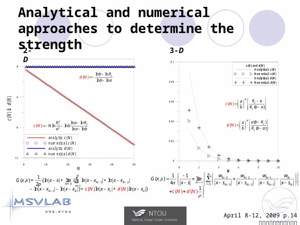
April 8-12, 2009 p.14海大陳正宗終身特聘教授
Analytical and numerical approaches to determine the strength
2-D 3-D
0 10 20 30 40 50
N
-12
-8
-4
0
c(N
) &
d(N
)
an a ly tic c (N )n u m erica l c (N )an a ly tic d (N )n u m erica l d (N )
0 2 4 6 8 10
N
0
0.02
0.04
0.06
0.08
0.1c (N ) a n d d (N )
A n a ly tica l c (N )N u m er ica l c (N )A n a ly tica l d (N )N u m er ica l d (N )
4 3 4 21
4 1 4
1( , ) {ln lim ( ln ln
2ln ( )ln ) ln }( ) ln
N
i iN
m
i i c d
G x x
c N d N
x x
x x x x
x x x xp
x x x x
- -®¥=
-
= - + - + -
- - - - + - + -
å4 3 4 2 4 1 4
1 4 3 4 2 4 1 4
1 1( , ) lim
4
( ) ( )1
Ni i i i
Ni i i i i
w w w wG x s
x s x s x s x s x s
c N d N
2
2
ln lnln ln( )
ln ln
R ac
RN bN
a a b
ln ln
n ln( )
l
b R
bd
aN
((
))
N R aa
b R b ac N
( )
(( )
)
N a b Rd
a
bN
b R a
April 8-12, 2009 p.15海大陳正宗終身特聘教授
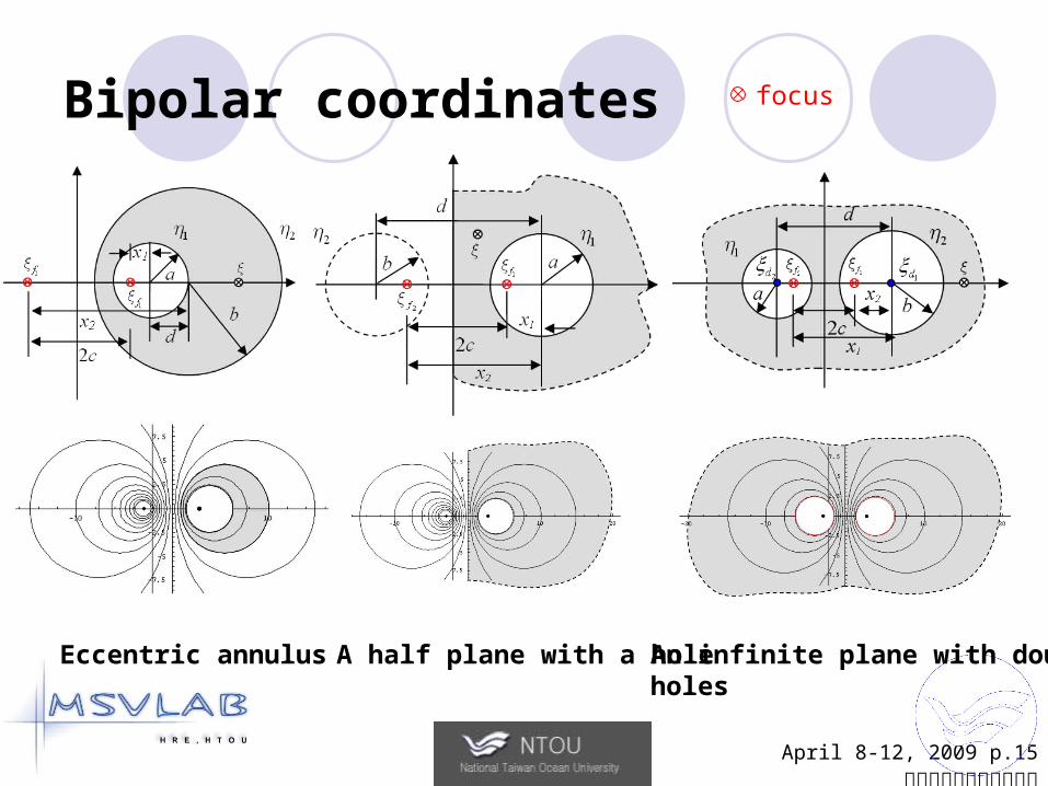
Bipolar coordinates
Eccentric annulus A half plane with a hole An infinite plane with double holes
focus
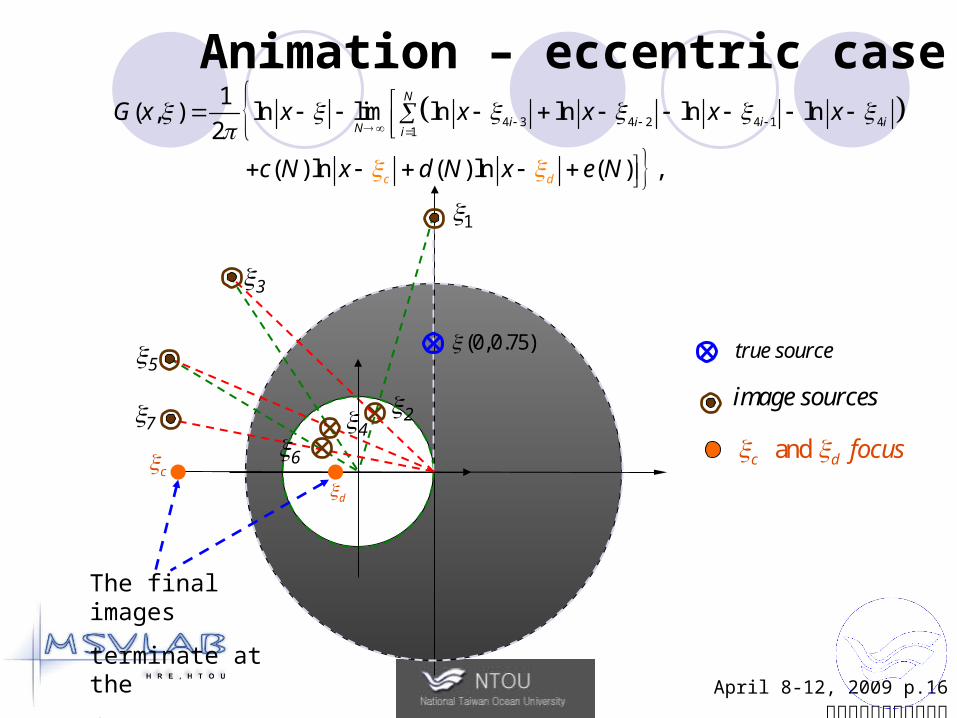
April 8-12, 2009 p.16海大陳正宗終身特聘教授
Animation – eccentric case
2
The final images
terminate at the
focus
46
7
1
5
3
(0,0.75)
4 3 4 2 4 1 41
1( , ) ln lim ln ln ln ln
2
( ) ln ( ) ln ( ) ,
N
i i i
c
iN
d
iG x x x x x x
c N x d N x e N
c
true source
image sources
and c d focus
d
April 8-12, 2009 p.17海大陳正宗終身特聘教授
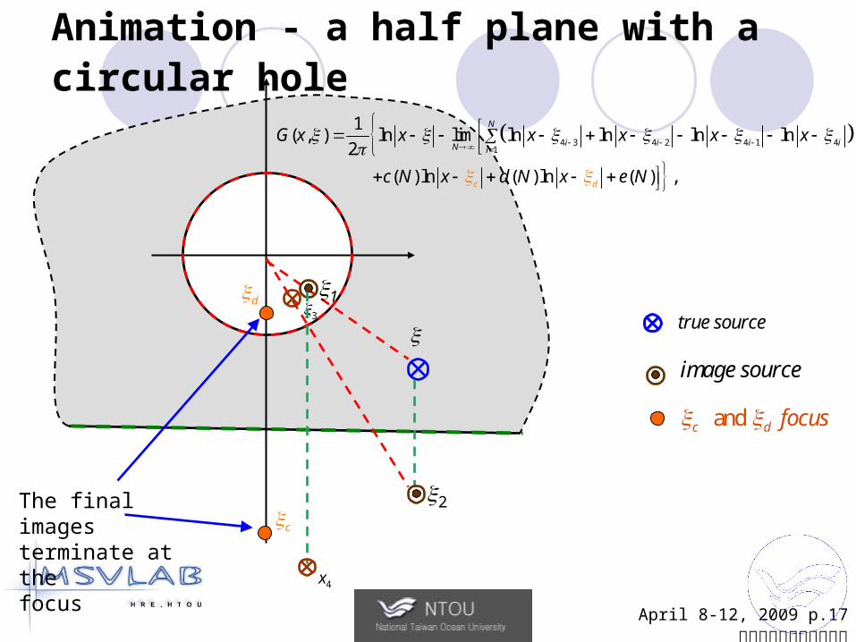
Animation - a half plane with a circular hole
1
2
3
4x
The final imagesterminate at thefocus
4 3 4 2 4 1 41
1( , ) ln lim ln ln ln ln
2
( ) ln ( ) ln ( ) ,
N
i i i
c
iN
d
iG x x x x x x
c N x d N x e N
d
c
image source
true source
and c d focus
April 8-12, 2009 p.18海大陳正宗終身特聘教授
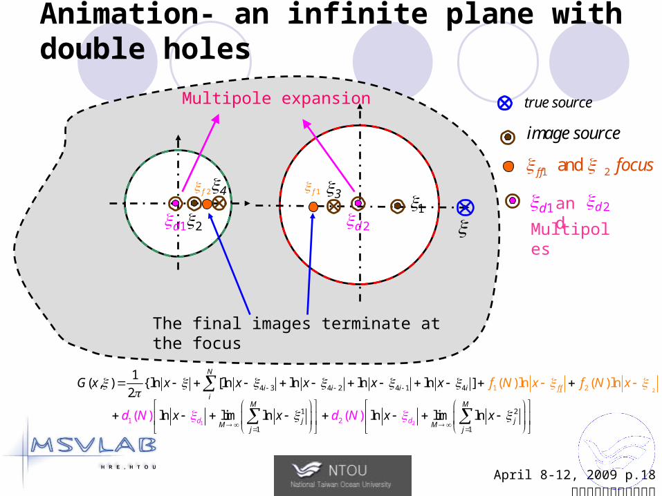
Animation- an infinite plane with double holes
1
234
The final images terminate at the focus
1d 2d
Multipole expansion
1
1
2
2
4 3 4 2 4 1 4
11
2
12
1
2
1
( ) ( )
1( , ) {ln [ln ln ln ln ]
2
ln lim ln ln
( )ln (
m
n
l
l
li n
)N
i i i ii
M
f f
d d
M
j jM M
j j
d
G x x f Nx x x f Nx x
x x N xN
x
xd
1f2f
true source
1 2 and f f focus
image source
2dand1dMultipoles
April 8-12, 2009 p.19海大陳正宗終身特聘教授
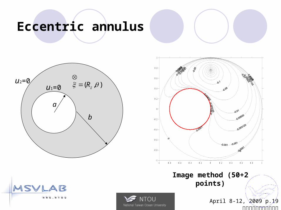
Eccentric annulus
- 1 - 0 . 8 - 0 . 6 - 0 . 4 - 0 . 2 0 0 . 2 0 . 4 0 . 6 0 . 8 1- 1
- 0 . 8
- 0 . 6
- 0 . 4
- 0 . 2
0
0 . 2
0 . 4
0 . 6
0 . 8
1
Image method (50+2 points)
u1=0u2=0 ),( R
a
b
April 8-12, 2009 p.20海大陳正宗終身特聘教授
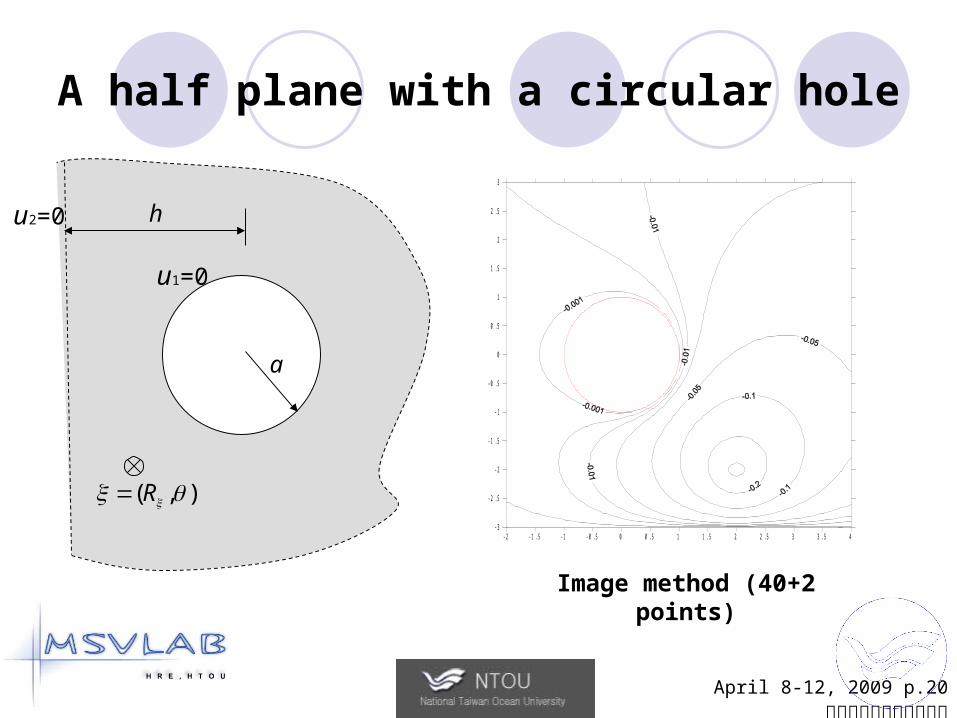
A half plane with a circular hole
-2 -1.5 -1 -0.5 0 0.5 1 1.5 2 2.5 3 3.5 4-3
-2.5
-2
-1.5
-1
-0.5
0
0.5
1
1.5
2
2.5
3
Image method (40+2 points)
u1=0
u2=0
),( R
a
h
April 8-12, 2009 p.21海大陳正宗終身特聘教授
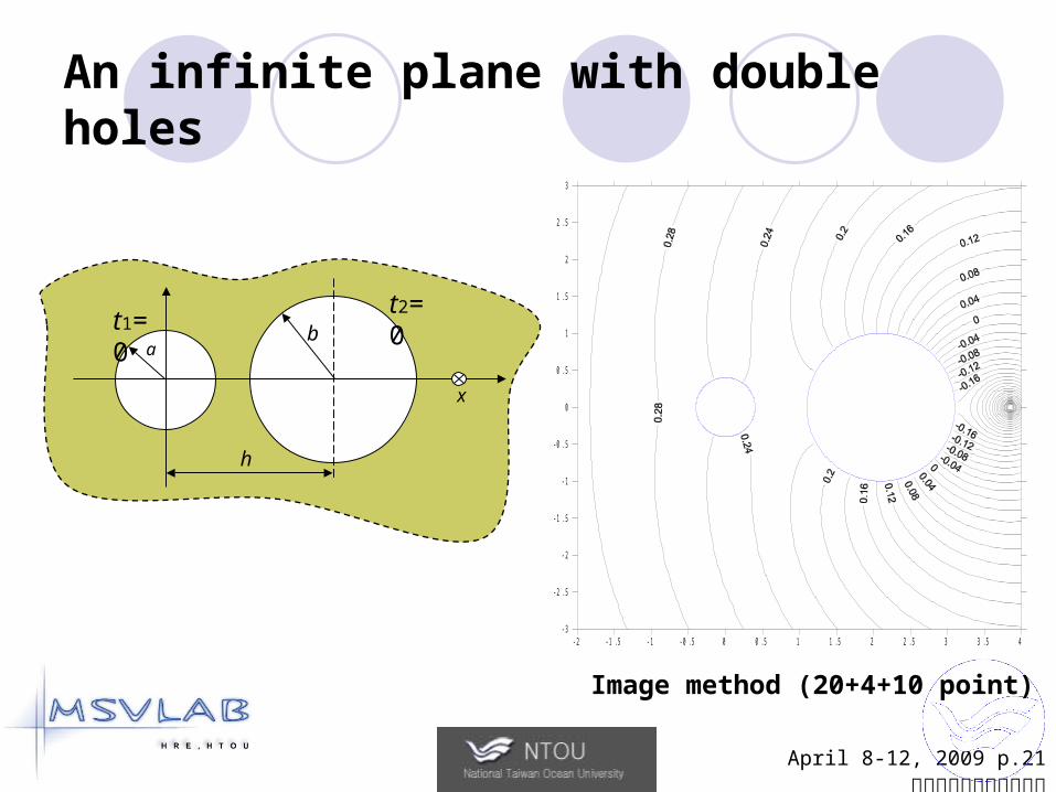
An infinite plane with double holes
ab
h
x
-2 -1.5 -1 -0.5 0 0.5 1 1.5 2 2.5 3 3.5 4-3
-2.5
-2
-1.5
-1
-0.5
0
0.5
1
1.5
2
2.5
3
Image method (20+4+10 point)
t1=0t2=0
April 8-12, 2009 p.22海大陳正宗終身特聘教授
Conclusions
The analytical solutions derived by the Trefftz method and MFS were proved to be mathematically equivalent for the annular Green’s functions (2D and 3D) after using addition theorem (degenerate kernel).
We can find final two frozen image points which are focuses in the bipolar coordinates.
The image idea provides the optimal location of MFS and only at most 4 by 4 matrix is required.
1. Introduction2. Problem statements3. Present method
4. Equivalence of Trefftz and MFS
5. Numerical examples6. Conclusions

April, 8-12, 2009 p.23海大陳正宗終身特聘教授
Thanks for your kind attentions
You can get more information from our website
http://msvlab.hre.ntou.edu.tw/
April 8-12, 2009 p.24海大陳正宗終身特聘教授
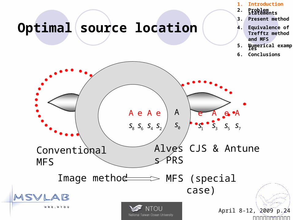
Optimal source location
0s
Ä
1s
e
2s
e
3s
Ä
4s
Ä
5s
e
6s
e
7s
Ä
8s
Ä
1. Introduction2. Problem statements3. Present method
4. Equivalence of Trefftz method and MFS
5. Numerical examples6. Conclusions
MFS (special case)Image method
Conventional MFS Alves CJS & Antunes PRS
April 8-12, 2009 p.25海大陳正宗終身特聘教授
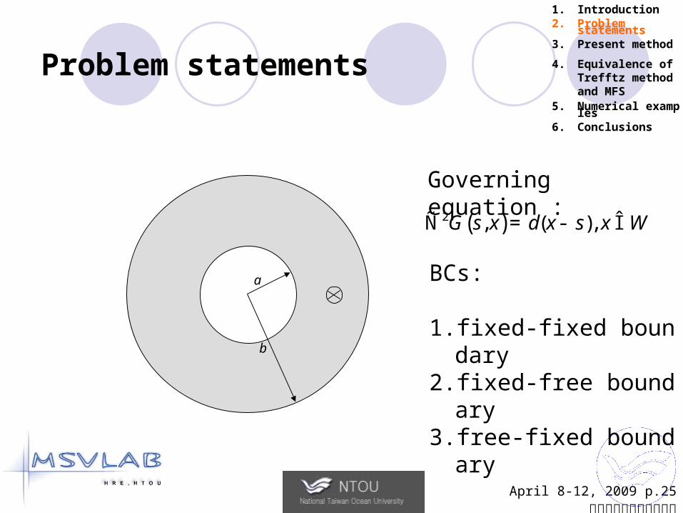
Problem statements
a
b
Governing equation :
( )2 , ( ),G s x x s xd WÑ = - Î
BCs:
1. fixed-fixed boundary2. fixed-free boundary3. free-fixed boundary
1. Introduction2. Problem statements3. Present method
4. Equivalence of Trefftz method and MFS
5. Numerical examples6. Conclusions
April 8-12, 2009 p.26海大陳正宗終身特聘教授
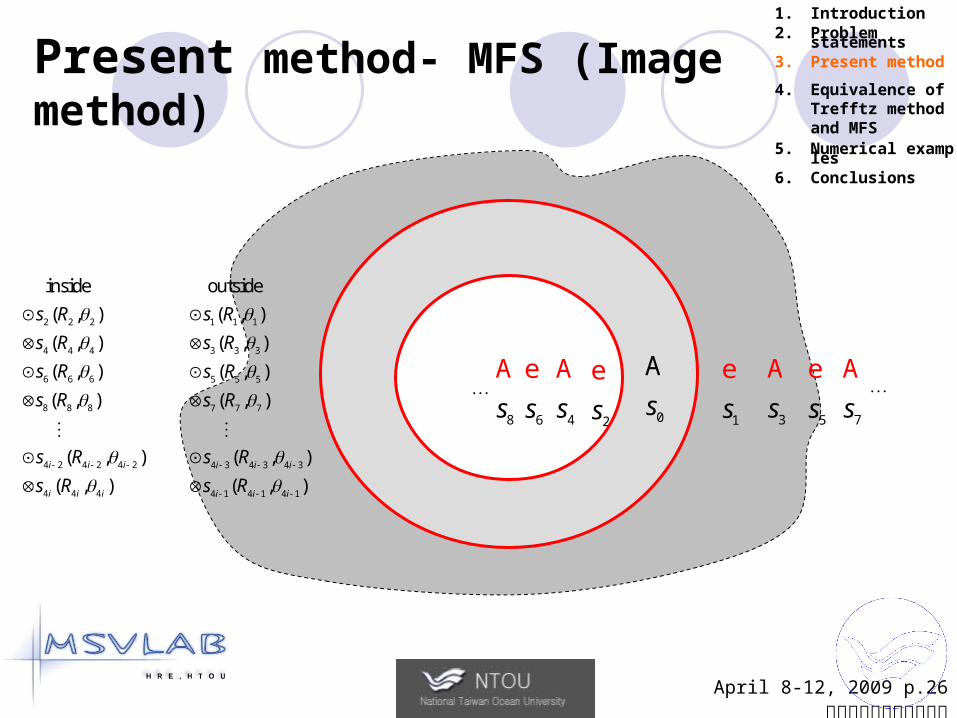
Present method- MFS (Image method)
0s
Ä
1s
e
2s
e
3s
Ä
4s
Ä
5s
e
6s
e
7s
Ä
8s
Ä
2 2 2
4 4 4
6 6 6
8 8 8
4 2 4 2 4 2
4 4 4
inside
( , )
( , )
( , )
( , )
( , )
( , )i i i
i i i
s R
s R
s R
s R
s R
s R
1 1 1
3 3 3
5 5 5
7 7 7
4 3 4 3 4 3
4 1 4 1 4 1
outside
( , )
( , )
( , )
( , )
( , )
( , )i i i
i i i
s R
s R
s R
s R
s R
s R
1. Introduction2. Problem statements3. Present method
4. Equivalence of Trefftz method and MFS
5. Numerical examples6. Conclusions
April 8-12, 2009 p.27海大陳正宗終身特聘教授
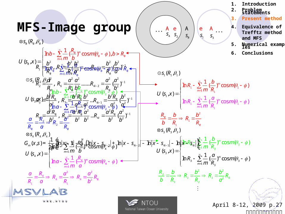
MFS-Image group0s
ee1s
Ä
3s4s ÄÄ
00
0
0 0 0
1 0
0
01
0 0
1ln ( ) c
1ln ( ) c
( , )
(os ( )
,
os (
),
),m
m
m
m
aR m
s R
U s
Rb m b
a
Rb
m R
m
Rx
1 11 1
2
0
1 11
1 1 1
1
1
1 0
1
1ln ( ) cos (
1ln ( ) cos (
(
( ,
)
)
)
, )
m
m
m
m
aR
b
m
s
R mm R
R b bR
b R R
m R
R
U s x
22
1
2 2 2
2
22
1
2
22
0 0
1ln ( ) cos (
1ln ( ) cos
( ,
(
)
( , ))
)
m
m
m
m
Ra
R
m
s
b mm
m a
a R aR
R a R
U x b
R
s
44
1
2 2
44 4 02
1 1
4 4 4
44
1
4
( , )
1ln (
1ln ( ) cos
) co
(
s )
)
(( , )
m
m
m
m
Ra m
m a
a R a aR R R
R a R b
s R
Rb m
m bU s x
3 31 3
2 2
23 3 02
3 3 3
3
3 31 3
3 2
( , )
( , )1
ln ( ) cos (
1ln ( ) ( )
)
cos
m
m
m
m
bR m
m R
R b b bR R R
s R
U s xa
R mm R
b R R a
2s
2 2 2 2 21
1 5 4 32 2
0 0 0
2 2 2 2 21
2 6 4 22 2
0 0 0
2 2 2 2 210 0 0
3 7 4 12 2 2 2 2
2 2 2 2 210 0 0
4 8 42 2 2 2 2
, ........ ( )
, ....... ( )
, ... ( )
, ... ( )
i
i
i
i
i
i
i
i
b b b b bR R R
R R a R a
a a a a aR R R
R R b R b
b R b R b b R bR R R
a a a a aa R a R a a R a
R R Rb b b b b
( )4 3 4 2 4 1 41
1( , ) ln ln ln ln ln
2
N
m i i i ii
G x s x s x s x s x s x s- - -=
é ù= - - - + - - - - -åê ú
pë û
1. Introduction2. Problem statements3. Present method
4. Equivalence of Trefftz method and MFS
5. Numerical examples6. Conclusions
April 8-12, 2009 p.28海大陳正宗終身特聘教授
Analytical derivation
1. Introduction2. Problem statements3. Present method
4. Equivalence of Trefftz method and MFS
5. Numerical examples6. Conclusions
April 8-12, 2009 p.29海大陳正宗終身特聘教授
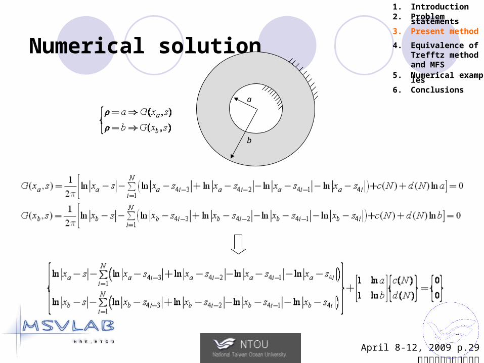
Numerical solution
1. Introduction2. Problem statements3. Present method
4. Equivalence of Trefftz method and MFS
5. Numerical examples6. Conclusions
a
b

April 8-12, 2009 p.30海大陳正宗終身特聘教授
Interpolation functions
a
b
1. Introduction2. Problem statements3. Present method
4. Equivalence of Trefftz method and MFS
5. Numerical examples6. Conclusions
April 8-12, 2009 p.31海大陳正宗終身特聘教授
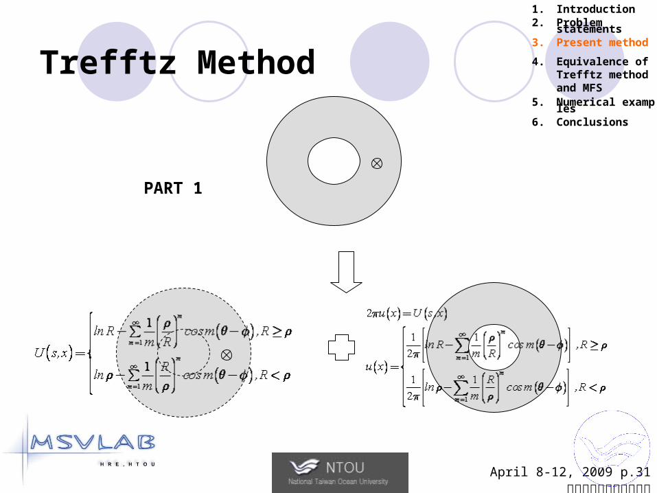
Trefftz Method
PART 1
1. Introduction2. Problem statements3. Present method
4. Equivalence of Trefftz method and MFS
5. Numerical examples6. Conclusions
April 8-12, 2009 p.32海大陳正宗終身特聘教授
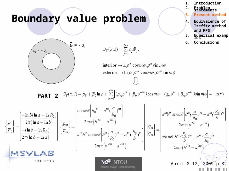
Boundary value problem
1 1u u=-2 2u u=-
PART 2
1. Introduction2. Problem statements3. Present method
4. Equivalence of Trefftz method and MFS
5. Numerical examples6. Conclusions
April 8-12, 2009 p.33海大陳正宗終身特聘教授
1u
2u11 uu
22 uu 1 0u =
2 0u =
PART 1 + PART 2 :
( )
( )
( )
1
1
0 01
( , )
1 1ln cos ,
2
1 1ln cos ,
2
1( ) ln ( cos ( sin
2
m
m
m
m
m m m mm m m m
m
G x s u u
R m Rm R
u xR
m Rm
u x p p p p ) m q q ) m
rq f r
p
r q f rp r
r r r f r r fp
¥
=
¥
=
¥ - -
=
= +
ì é ùï æ öï ê ú÷çï - - ³å ÷çï ê ú÷çè øï ê úï ë ûï=í é ùï æ öï ê ú÷çï - - <÷å çï ê ú÷ç ÷ï è øê úï ë ûïîì üï ïï é ù= + + + + +åí ýê úë ûïïî
ïïïþ
1. Introduction2. Problem statements3. Present method
4. Equivalence of Trefftz method and MFS
5. Numerical examples6. Conclusions
April 8-12, 2009 p.34海大陳正宗終身特聘教授
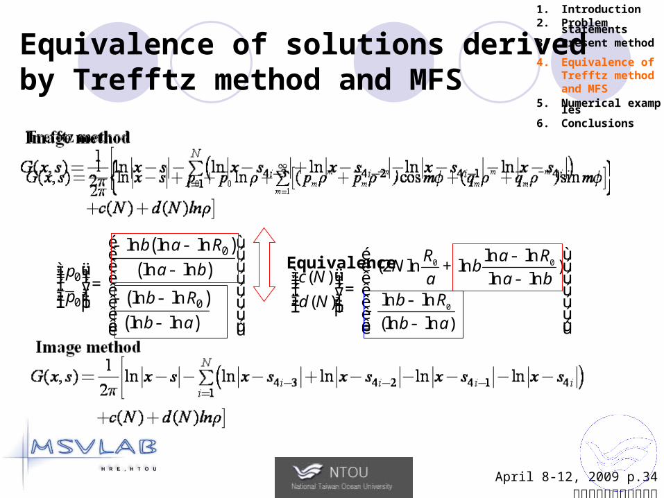
Equivalence of solutions derived by Trefftz method and MFS
1. Introduction2. Problem statements3. Present method
4. Equivalence of Trefftz method and MFS
5. Numerical examples6. Conclusions
Equivalence ( )
( )( )( )
0
0
0 0
ln ln ln
ln ln
ln ln
ln ln
b a R
a bp
p b R
b a
é ù- -ê úê úì ü -ï ïï ï ê ú=í ý ê úï ï - -ï ï ê úî þê ú-ê úë û
0 0
0
ln ln(2 ln ln )
( ) ln lnln ln( )(ln ln )
R a RN b
c N a a bb Rd Nb a
é ù-ê ú- +ì ü ê úï ï -ï ï =ê úí ý -ï ï ê úï ïî þ -ê ú
-ê úë û
April 8-12, 2009 p.35海大陳正宗終身特聘教授
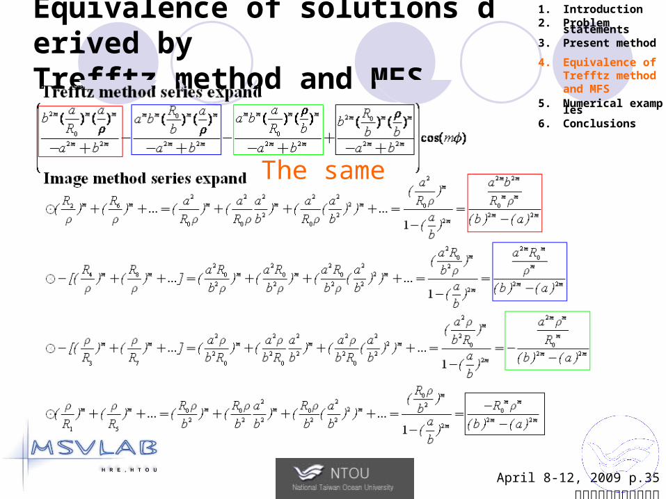
The same
1. Introduction2. Problem statements3. Present method
4. Equivalence of Trefftz method and MFS
5. Numerical examples6. Conclusions
Equivalence of solutions derived by Trefftz method and MFS
April 8-12, 2009 p.36海大陳正宗終身特聘教授
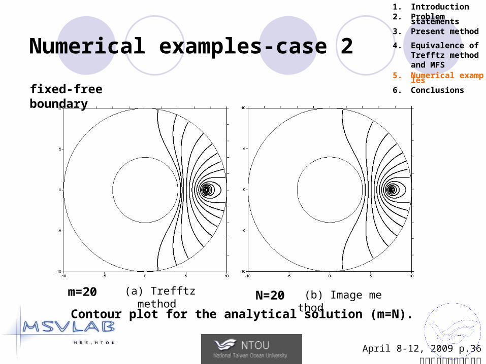
Numerical examples-case 2
(a) Trefftz method (b) Image method
Contour plot for the analytical solution (m=N).
fixed-free boundary
1. Introduction2. Problem statements3. Present method
4. Equivalence of Trefftz method and MFS
5. Numerical examples6. Conclusions
m=20 N=20
April 8-12, 2009 p.37海大陳正宗終身特聘教授
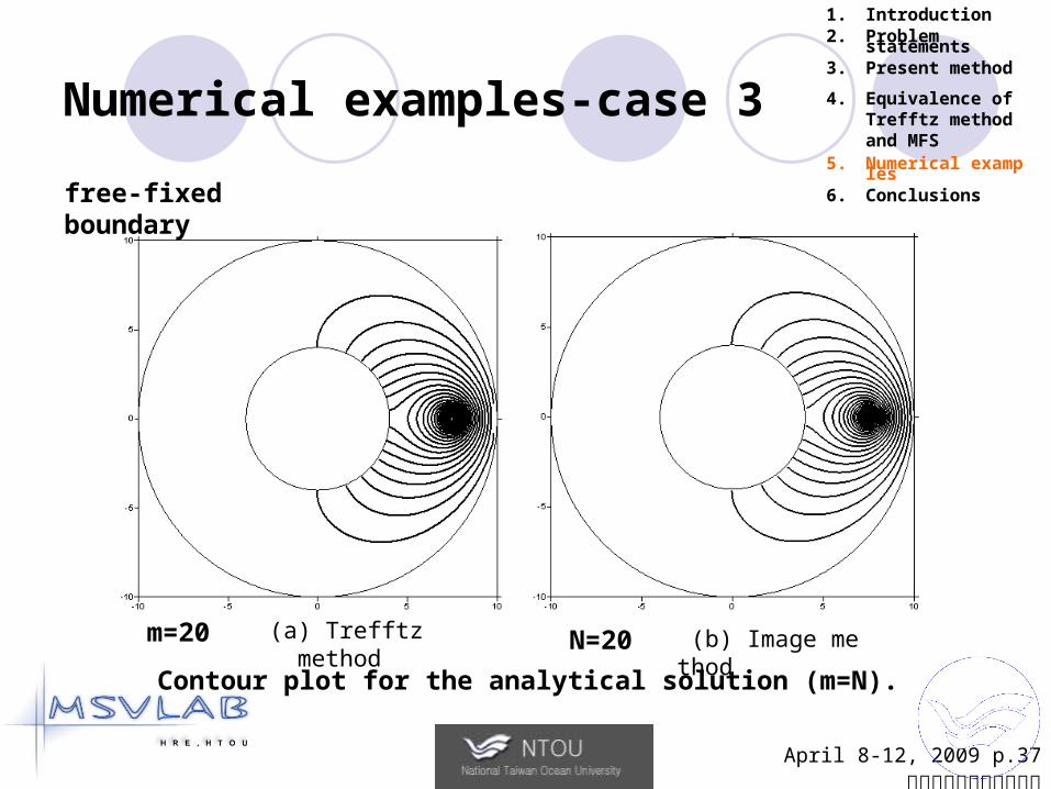
Numerical examples-case 3
(a) Trefftz method (b) Image method
Contour plot for the analytical solution (m=N).
free-fixed boundary
1. Introduction2. Problem statements3. Present method
4. Equivalence of Trefftz method and MFS
5. Numerical examples6. Conclusions
m=20 N=20
April 8-12, 2009 p.38海大陳正宗終身特聘教授
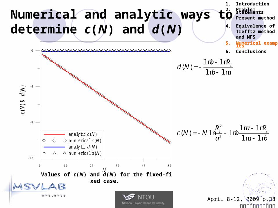
Numerical and analytic ways to determine c(N) and d(N)
Values of c(N) and d(N) for the fixed-fixed case.
1. Introduction2. Problem statements3. Present method
4. Equivalence of Trefftz method and MFS
5. Numerical examples6. Conclusions
0 10 20 30 40 50
N
-12
-8
-4
0
c(N
) &
d(N
)
an a ly tic c (N )n u m erica l c (N )an a ly tic d (N )n u m erica l d (N )
ba
Rab
a
RNNc
lnln
lnlnlnln)(
2
2
ab
RbNd
lnln
lnln)(
April 8-12, 2009 p.39海大陳正宗終身特聘教授
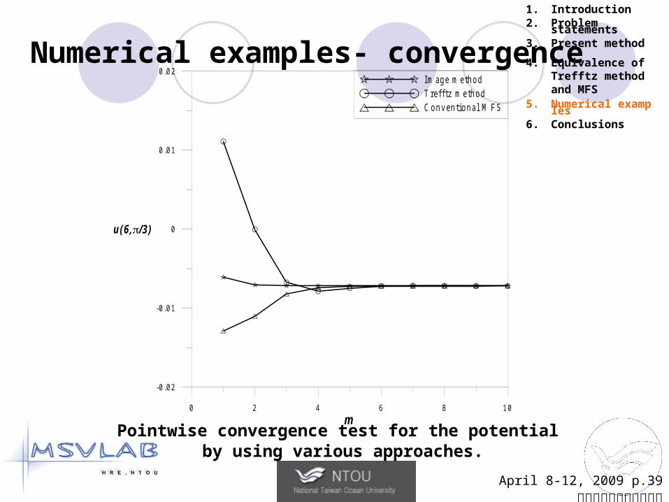
Numerical examples- convergence
1. Introduction2. Problem statements3. Present method
4. Equivalence of Trefftz method and MFS
5. Numerical examples6. Conclusions
Pointwise convergence test for the potential by using various approaches.
0 2 4 6 8 10
m
-0 .02
-0.01
0
0.01
0.02
u (6 ,/3 )
Im a g e m e th o dT re fftz m e th o dC o n v en tio n a l M F S