ctryu14

7/25/2019 ctryu14

http://slidepdf.com/reader/full/ctryu14 1/35

Control Systems Lab – SC4070

Lecture 3, February 22, 2013

dr.ir. Alessandro Abate

Delft Center for Systems and Control

Delft University of Technology

The Netherlands

e-mail: [email protected]

tel: 015 27 85606

(slides modified from the original, drafted by Robert Babuska)

7/25/2019 ctryu14


Lecture outline

• Overview of control design methods

• Continuous vs. discrete time design• State-feedback control, observers

• Control architectures, nonlinear control

• PID controllers

7/25/2019 ctryu14


Linear control design methods

• P, PD, PI, PID, lead-lag control (classical, in frequency)

• state feedback, output feedback (modern, in state-space)

• LQR, linear quadratic control (optimal)

• model predictive control (optimal, finite-horizon, constrained)

• robust control ( H ∞, µ−synthesis)

7/25/2019 ctryu14


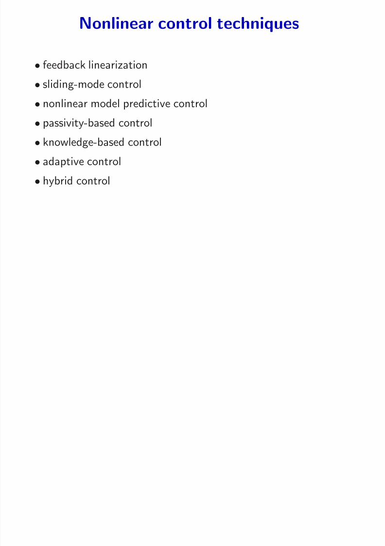
Nonlinear control techniques

• feedback linearization

• sliding-mode control

• nonlinear model predictive control

• passivity-based control

• knowledge-based control

• adaptive control

• hybrid control

7/25/2019 ctryu14


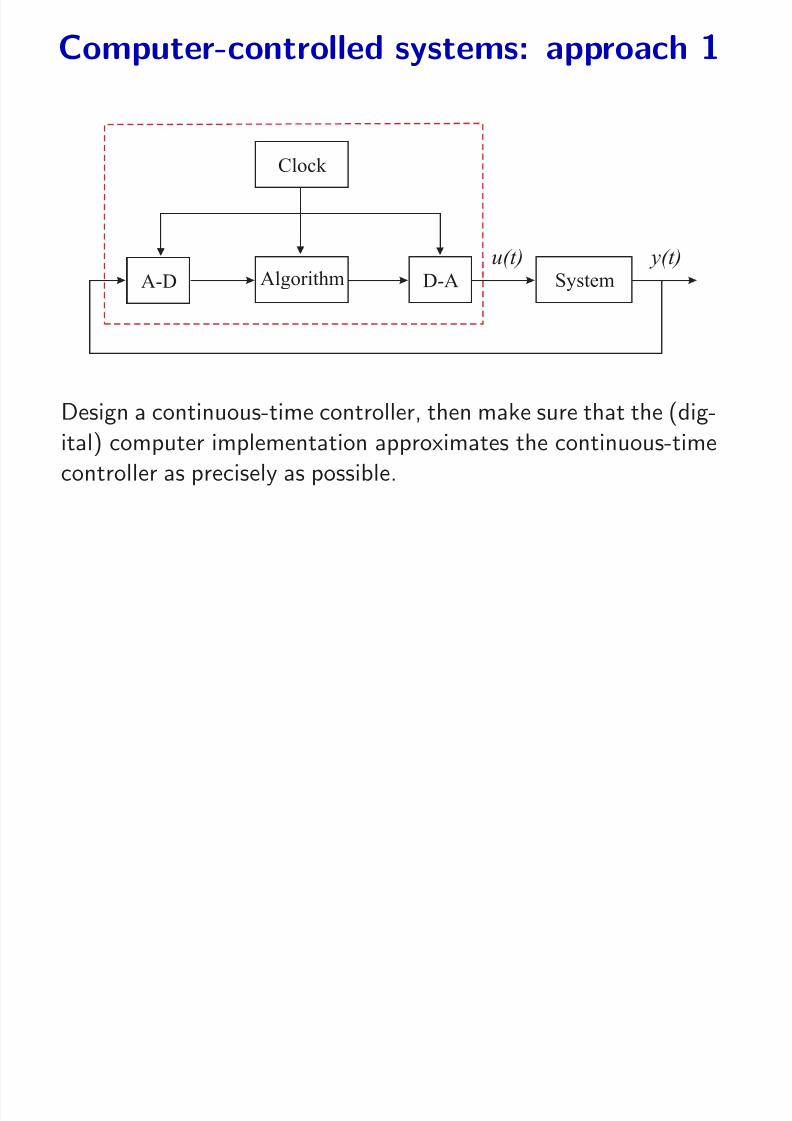
Computer-controlled systems: approach 1

y(t)u(t)Algorithm

Clock

A-D D-A System

Design a continuous-time controller, then make sure that the (dig-

ital) computer implementation approximates the continuous-time

controller as precisely as possible.

7/25/2019 ctryu14


Computer-controlled systems: approach 2

y(t)u(t)Algorithm

Clock

A-D D-A System

Describe the system from the computer’s (digital) viewpoint and

design directly a discrete-time controller.

7/25/2019 ctryu14


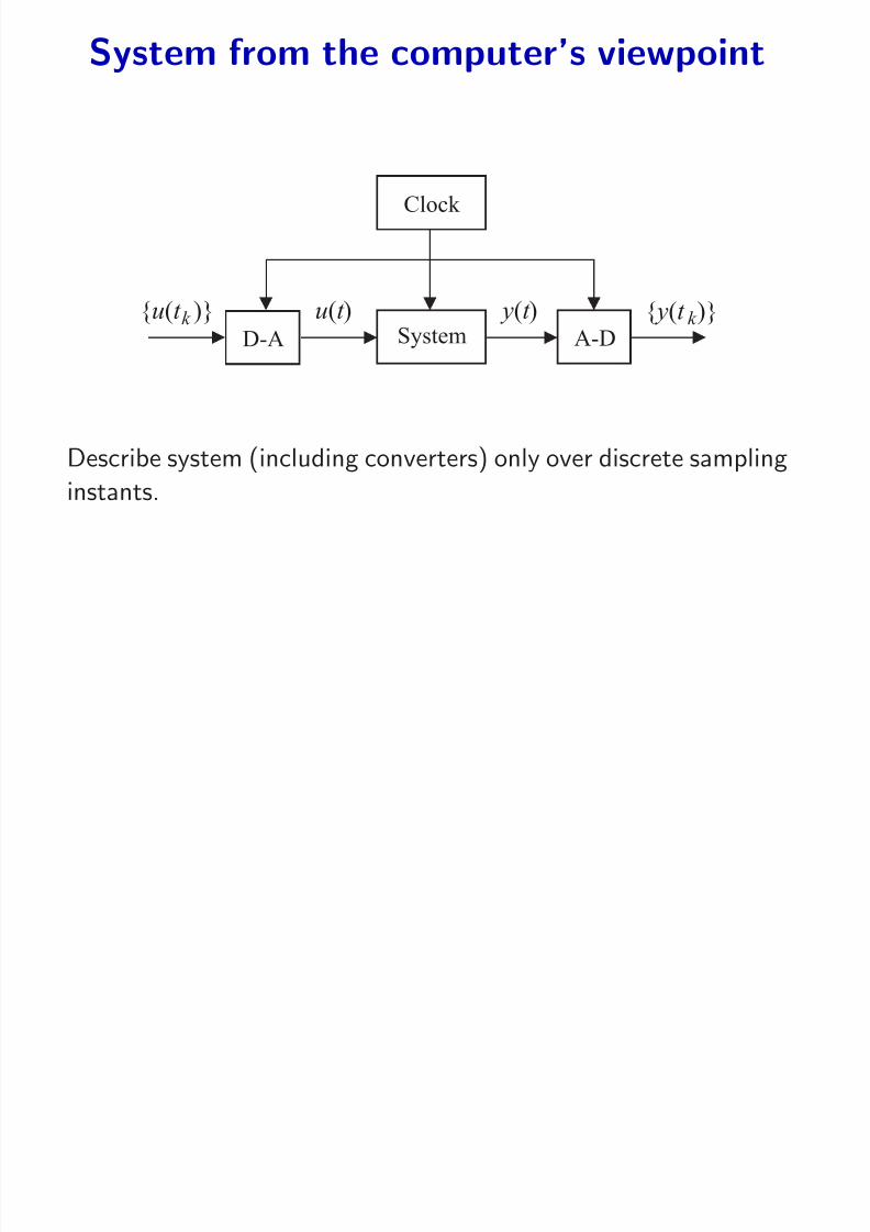
System from the computer’s viewpoint

y t ( )u t ( ) System

Clock

{ ( )} y t k { ( )}u t k A-DD-A

Describe system (including converters) only over discrete sampling

instants.

7/25/2019 ctryu14


A-D Converter: Zero-Order Hold

Timet t t t t t 0 1 2 3 4 5

u(t ) = u(t k ), t k ≤ t < t k +1

Usually (but not necessarily) t k +1− t k = const = h.

Higher-order converters are also possible.

7/25/2019 ctryu14


Zero-order hold sampling of systems

Continuous-time system:

dx(t )

dt

= Ax(t ) + Bu(t )

y(t ) = Cx(t ) + Du(t )

Discrete-time system:

x(k + 1) = Φ x(k ) +Γ u(k ) y(k ) = Cx(k ) + Du(k )

with (recall solution of non-autonomous ODE):

Φ = e Ah , Γ =

h

0

e AsdsB, where h is the sampling period

Reflect on eigenvalues placement

7/25/2019 ctryu14


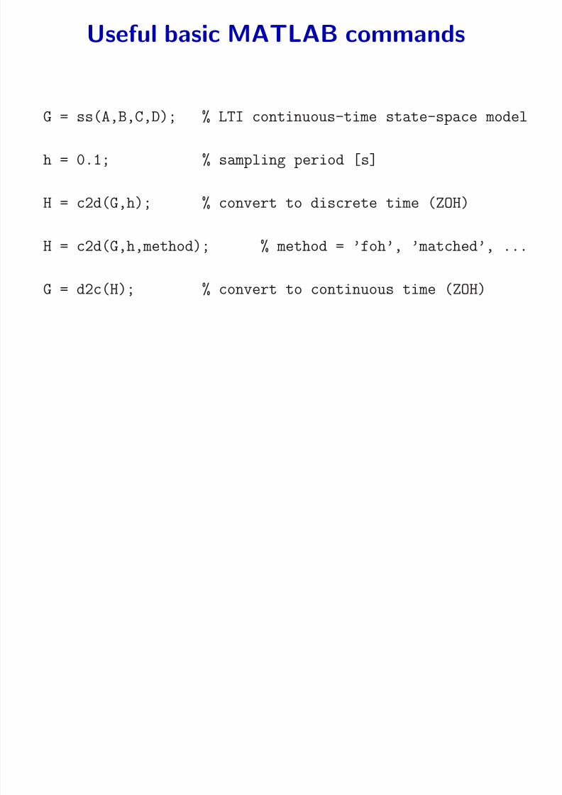
Useful basic MATLAB commands

G = ss(A,B,C,D); % LTI continuous-time state-space model

h = 0.1; % sampling period [s]

H = c2d(G,h); % convert to discrete time (ZOH)

H = c2d(G,h,method); % method = ’foh’, ’matched’, ...

G = d2c(H); % convert to continuous time (ZOH)

7/25/2019 ctryu14


Selection of sampling period (1st order)

Number of samples per rise time: N r = T r

h ≈ 4−10

0 5

−1

0

1(a)

0 50

1

0 5

−1

0

1(b)

0 50

1

0 5

−1

0

1(c)

0 50

1

0 5

−1

0

1(d)

Time

0 50

1

Time

(a) N r = 1

(b) N

r = 2

(c) N r = 4

(d) N r = 8

7/25/2019 ctryu14


Selection of sampling period (2nd order)

N r = T r

h ≈ 4−10 corresponds to ω0h ≈ 0.2−0.5

0 50

1

(a)

0 50

1

(b)

0 50

1

(c)

Time

0 50

1

(d)

Time

(a) h = 0.125 (ω0h = 0.23), (b) h = 0.250 (ω0h = 0.46),

(c) h = 0.500 (ω0h = 0.92), (d) h = 1.000 (ω0h = 1.83)

7/25/2019 ctryu14


State feedback in DT: problem formulation

• Discretize LTI model choosing a sampling interval

• Model : x(k + 1) = Φ x(k ) +Γ u(k )

• Linear controller :

u(k ) = − Lx(k )

• Design parameters: closed-loop poles

• Evaluation: compare x(k ) and u(k ) with specifications

(trade-off between control magnitude and speed of response)

7/25/2019 ctryu14


Poles placement: Ackermann formula

Compute L such that (Φ−Γ L) has a desired characteristic poly-

nomial P( z). Ackermann formula:

L = (0 . . . 0 1)W −1c P(Φ)

where P(Φ) is the desired characteristic polynomial in Φ

Place poles inside unit ball

In Matlab:

L = acker(Phi,Gamma,Po) (SISO, numerical problems ?)

L = place(Phi,Gamma,Po) (MISO, more robust)

7/25/2019 ctryu14


Alternatively, choice of desired poles in CT

Use the continuous-time 2nd order model, study char. pol.:

s

2

+ 2ζωs +ω2

,

which leads to z2 + p1 z + p2 with

p1 = −2e−ζωh cosωh

1−ζ2

p2 = e−2ζωh

Thereafter in Matlab use c2d for closed-loop model

7/25/2019 ctryu14


Linear quadratic control: LQR

J = N

∑k =1

x(k )T Qx(k ) + u(k )T Ru(k ),

where (matrices, weights) Q, R are design parameters

A state feedback matrix L that gives a minimal J can be found by

solving the Riccati equation.

Similar to pole placement, but no need to define poles!

In Matlab: dlqr(Phi,Gamma,Q,R) % state weighting

In Matlab: dlqry(Phi,Gamma,C,D,Q,R) % output weighting

7/25/2019 ctryu14


State estimation: observers

x(k + 1) = Φ x(k ) +Γ u(k )

y(k ) = Cx(k )

Assume input and output are available, reconstruct the state:

• Direct calculation

• Luenberger observer (model-based)

• Kalman filter (optimal in presence of noise)

Note: the terms “observer”, “estimator”, “filter” are in this con-

text used synonymously

7/25/2019 ctryu14


State reconstruction based on a model

Consider the model: ˆ x(k + 1) = Φ ˆ x(k ) +Γ u(k )

7/25/2019 ctryu14


Model-based state estimation


Introduce “feedback” term from measured y(k )

ˆ x(k + 1) = Φ ˆ x(k ) +Γ u(k ) + K [ y(k )−C x(k )]

7/25/2019 ctryu14


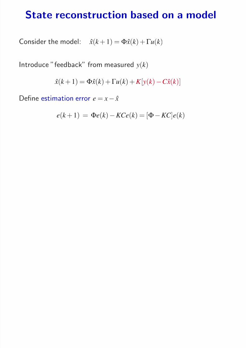
State reconstruction based on a model


Introduce ”feedback” from measured y(k )

ˆ x(k + 1) = Φ ˆ x(k ) +Γ u(k ) + K [ y(k )−C x(k )]

Define estimation error e = x− ˆ x

e(k + 1) = Φe(k )−KCe(k ) = [Φ−KC ]e(k )

7/25/2019 ctryu14


Observer – block diagram

K

1z

u k ( ) x k+( 1)^

y k ( )^

y k ( )

C x k ( )^

x k ( )^

7/25/2019 ctryu14


Output feedback (observer + state feedback)

ˆ x(k + 1) = Φ ˆ x(k ) +Γ u(k ) + K

y(k )−C x(k )

u(k ) = − L ˆ x(k )

7/25/2019 ctryu14


Poles of the closed-loop system

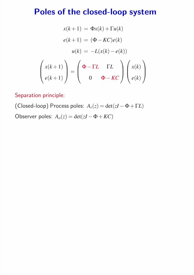
x(k + 1) = Φ x(k ) +Γ u(k )

e(k + 1) = (Φ−KC )e(k )

u(k ) = − L( x(k )− e(k ))

7/25/2019 ctryu14



x(k + 1) = Φ x(k ) +Γ u(k )

e(k + 1) = (Φ−KC )e(k )

u(k ) = − L( x(k )− e(k ))

x(k + 1)

e(k + 1)

=Φ−Γ L Γ L

0 Φ−KC

x(k )

e(k )

7/25/2019 ctryu14



x(k + 1) = Φ x(k ) +Γ u(k )

e(k + 1) = (Φ−KC )e(k )

u(k ) = − L( x(k )− e(k ))

x(k + 1)

e(k + 1)

=Φ−Γ L Γ L

0 Φ−KC

x(k )

e(k )

Separation principle:(Closed-loop) Process poles: Ar ( z) = det( zI −Φ+Γ L)

Observer poles: Ao( z) = det( zI −Φ+ KC )

7/25/2019 ctryu14


Feed-forward (two-degree-of-freedom)

Goal: respond to a reference signal with desired specs.Replace u(k ) = − L ˆ x(k ) by: u(k ) = − L ˆ x(k ) + Lcuc(k )

u x^

Lc

Observer

Process-L

uc

y

7/25/2019 ctryu14


Feed-forward (two-degree-of-freedom)

Closed-loop system:

x(k + 1) = (Φ−Γ L) x(k ) +Γ Le(k ) +Γ Lcuc(k )

e(k + 1) = (Φ−KC )e(k )

y(k ) = Cx(k )

Transfer function from uc to y (for impulse response):

H cl( z) = C ( zI −Φ+Γ L)−1Γ Lc = Lc

B( z)

Ar ( z)

A li i li

7/25/2019 ctryu14


Application to a nonlinear system

Feedback controller

Reference Nonlinear system

y0

y

u0

y0

Feedforward controller

C l b l l li ll

7/25/2019 ctryu14


Control by local linear controller

u

u0

Linear controller

Nonlinear

system

y0

y

Linearized

model

M d l b d d ti t l

7/25/2019 ctryu14


Model-based adaptive control

u

Adaptation

Design parameters

Controller

-

Process

Linear model

yr

ym

C ti ti PID t ll

7/25/2019 ctryu14


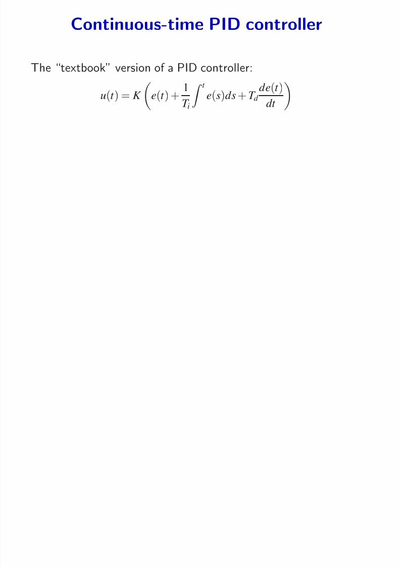
Continuous-time PID controller

The “textbook” version of a PID controller:

u(t ) = K

e(t ) +

1

T i

t

e(s)ds + T d

de(t )

dt

C ti ti PID t ll

7/25/2019 ctryu14


Continuous-time PID controller

The “textbook” version of a PID controller:

u(

t ) =

K e(

t ) +

1

T i

t

e(

s)

ds+

T d

de(t )

dt

A more realistic PID controller:

U (s) = K

(U c(s)−

Y (s)) +

1

sT i(U c(s)−

Y (s))−

sT d

1 + sT d / N Y (s)

Discrete time PID controller

7/25/2019 ctryu14


Discrete-time PID controller

P-term: P(k ) = K (uc(k )− y(k ))

I-term: I (k + 1) = I (k ) + K T ie(k )

D-term: D(k ) = T d

T d + Nh D(k −1)− KT d N

T d + Nh ( y(k )− y(k −1))

u(k ) = P(k ) + I (k ) + D(k )

PID tuning

7/25/2019 ctryu14


PID tuning

• Pole placement

• Root locus

• Bode diagram

• Tuning rules (Ziegler-Nichols, λ−tuning)

G(s) = e−t 0s K p

(τs + 1) ⇒ K c =

τ

K p(λ+ t 0), T i = τ, T d =

t 0

2

Cascaded control on an Inverted Pendulum

7/25/2019 ctryu14


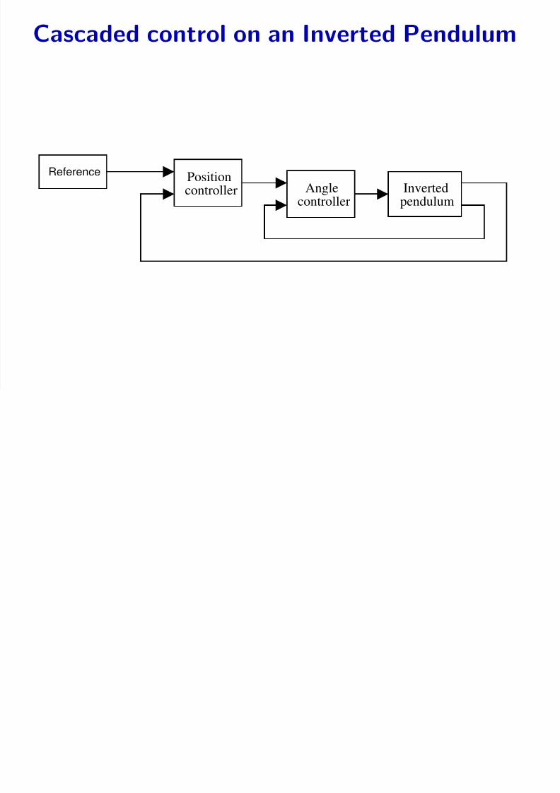
Cascaded control on an Inverted Pendulum

Reference Position controller Inverted

pendulumAngle

controller

ctryu14

Documents